Merge-split Markov chain Monte Carlo for community detection

Abstract

We present a Markov chain Monte Carlo scheme based on merges and splits of groups that is capable of efficiently sampling from the posterior distribution of network partitions, defined according to the stochastic block model (SBM). We demonstrate how schemes based on the move of single nodes between groups systematically fail at correctly sampling from the posterior distribution even on small networks, and how our merge-split approach behaves significantly better, and improves the mixing time of the Markov chain by several orders of magnitude in typical cases. We also show how the scheme can be straightforwardly extended to nested versions of the SBM, yielding asymptotically exact samples of hierarchical network partitions.

I Introduction

Community detection Fortunato (2010) is an important tool for the analysis of network data, as it allows the breaking down of the network structure into basic building blocks, thus providing a summary of its large-scale structure. Among the many methods proposed for this task, those based on the statistical inference of generative models offer the most principled and robust choice Peixoto (2019a). This is due in large part to their ability to take into account and convey the statistical evidence available in the data, allowing us to prevent both overfitting — occurring when purely random fluctuations are mistaken by structure — as well as underfitting — occurring when statistically significant structure is mistaken by random fluctuations. These problems manifest themselves in nonstatistical methods in their tendency to identify spurious communities in fully random networks Guimerà et al. (2004) as well as those that are nonmodular but sparse Bagrow (2012), and in the failure at recognizing the existence of clear but relatively small communities in large networks Fortunato and Barthélemy (2007). The manner in which statistical inference allows us to overcome these obstacles is by allowing us to express not only our belief about how the data are generated, but also about how much information is needed to specify the model parameters. The combination of these two elements defines a posterior distribution of all possible community structures that are compatible with the data, ranked according to their plausibility. The posterior distribution inherently ascribes low probabilities to overly-complicated models, and yields the most parsimonious but sufficiently rich explanation for the data. Nevertheless, in case the model being used cannot perfectly encapsulate the structure in the data, the posterior distribution may still give comparatively high probabilities to multiple diverging explanations for the data. Choosing only one fit of the model, for example by selecting a single modular division with the strictly largest posterior probability, is a form of bias in this situation. Instead, it is preferable to consider the entire set of plausible partitions, by sampling from the posterior distribution, rather than maximizing it.

Although it is relatively easy to write down a mathematical expression for the posterior distribution of network partitions, at least up to a normalization constant, using a simple model family called the stochastic block model (SBM) Holland et al. (1983); Karrer and Newman (2011), actually sampling from this distribution is a different matter altogether. In fact, fitting the SBM in this way subsumes solving certain instances of combinatorial problems such as graph coloring that are known to be NP-hard, and indeed there is strong statistical evidence pointing to the existence of parameter regimes where, although it may be possible to characterize the posterior distribution of the SBM, this can only be done in nonpolynomial time Decelle et al. (2011). Because of this inherent intractability, it is unlikely that there will ever be an algorithm that samples directly from the posterior distribution in an efficient manner, at least not for networks that have more than a handful of nodes, as the number of possible partitions grows super-exponentially with network size. Nevertheless, we can still approach the problem in practice using approximate methods. One attractive choice is Markov chain Monte Carlo (MCMC), which consists in moving from one partition of the network to another, with a probability conditioned only on the current state, in a manner that guarantees exact asymptotic convergence to the desired posterior distribution, provided one is able to wait long enough for the chain to “mix.” In this way, one should be able to sample effectively from the posterior in feasible instances of the problem, which would correspond to a short mixing time.

In the case of the SBM, MCMC sampling has been implemented in a variety of ways Snijders and Nowicki (1997); Guimerà and Sales-Pardo (2009); Peixoto (2014a); Newman and Reinert (2016); Riolo et al. (2017), but all approaches thus far employed involve moves from one partition to another that differ only in the group membership of a single node. As we will show, these “single-node” approaches fail systematically at efficiently exploring the posterior distribution of partitions, as they cannot overcome low probability “barriers” that prevent the chain from mixing. This is particularly relevant in situations where the number of groups is unknown a priori, and the movement of a single node at a time forces the Markov chain to move through low-probability states composed of groups containing only one node, if the chain is to visit partitions with different numbers of groups. These stopgap transitions prevent the MCMC from mixing in a reasonable amount of time, and result in abysmal performance even in easy instances of the problem.

In this work we present an alternative MCMC scheme that involves the simultaneous movement of several nodes at each step, via the merging, splitting and re-arrangements of groups. As we show, these moves can easily overcome the low-probability barriers that block the single-move approaches, and cause the chain to mix several orders of magnitude faster. This improvement makes MCMC usable for significantly larger networks, and allows us to explore community structure in empirical networks with more confidence and increased amount of detail.

This paper is defined as follows. In Sec. II we briefly review the inference approach to community detection. In Sec. III.1 we describe the MCMC approach with single-node moves and in Sec. III.2 we describe the version with merges and splits. In Sec. IV we investigate the performance of both algorithms in empirical networks, and in Sec. V we extend the algorithm to hierarchical models. We end in Sec. VI with a conclusion.

II Bayesian inference of community structure

The inference approach to community detection involves first the stipulation of a generative model for the network structure given a network partition $\bm{b}=\{b_{1},\dots,b_{N}\}$, where $b_{i}\in[1,B]$ is the membership of node $i$ in one of $B$ groups. For example, when using the degree-corrected stochastic block model (DC-SBM) Karrer and Newman (2011), it is assumed that a network with adjacency matrix $\bm{A}$ is generated with probability

$$P(\bm{A}|\bm{\lambda},\bm{\theta},\bm{b})=\prod_{i<j}\frac{(\lambda_{b_{i}b_{j}}\theta_{i}\theta_{j})^{A_{ij}}\mathrm{e}^{-\lambda_{b_{i}b_{j}}\theta_{i}\theta_{j}}}{A_{ij}!}\times\\ \prod_{i}\frac{(\lambda_{b_{i}b_{i}}\theta_{i}^{2}/2)^{A_{ij}/2}\mathrm{e}^{-\lambda_{b_{i}b_{i}}\theta_{i}^{2}/2}}{(A_{ij}/2)!},$$ (1)

with the additional parameters $\bm{\lambda}$ and $\bm{\theta}$ specifying the affinity between groups and expected node degrees, respectively. The inference procedure consists in sampling from the posterior distribution

$$P(\bm{b}|\bm{A})=\frac{P(\bm{A}|\bm{b})P(\bm{b})}{P(\bm{A})},$$ (2)

where $P(\bm{b})$ is a prior probability of node partitions, and

$$P(\bm{A}|\bm{b})=\int P(\bm{A}|\bm{\lambda},\bm{\theta},\bm{b})P(\bm{\theta}|\bm{b})P(\bm{\lambda}|\bm{b})\;\mathrm{d}\bm{\theta}\mathrm{d}\bm{\lambda},$$ (3)

is the marginal likelihood integrated over the remaining model parameters, weighted according to their own prior probabilities. If we make a noninformative choice for them,

$$P(\bm{\theta}|\bm{b}) =\prod_{r}(n_{r}-1)!\,\delta\left(\textstyle\sum_{i}\theta_{i}\delta_{b_{i},r}-1\right),$$ (4)

$$P(\bm{\lambda}|\bm{b},\bar{\lambda}) =\prod_{r<s}\mathrm{e}^{-\lambda_{rs}/\bar{\lambda}}/\bar{\lambda}\prod_{r}\mathrm{e}^{-\lambda_{rs}/2\bar{\lambda}}/2\bar{\lambda},$$ (5)

we can compute the integral exactly as Peixoto (2017)

$$P(\bm{A}|\bm{b})=\frac{\bar{\lambda}^{E}}{(\bar{\lambda}+1)^{E+B(B+1)/2}}\times\\ \frac{\prod_{r<s}e_{rs}!\prod_{r}e_{rr}!!}{\prod_{i<j}A_{ij}!\prod_{i}A_{ii}!!}\prod_{r}\frac{(n_{r}-1)!}{(e_{r}+n_{r}-1)!}\prod_{i}k_{i}!,$$ (6)

where $e_{rs}=\sum_{ij}A_{ij}\delta_{b_{i},r}\delta_{b_{j},s}$, $e_{r}=\sum_{s}e_{rs}$, and $n_{r}=\sum_{i}\delta_{b_{i},r}$. The last remaining quantity

$$P(\bm{A})=\sum_{\bm{b}}P(\bm{A}|\bm{b})P(\bm{b})$$ (7)

is called the evidence, and servers as a normalization constant for the posterior distribution. Although it has an important role in the context of model selection, its value cannot be computed in closed form in the general case. Luckily this is not needed for MCMC, as we will shortly see.

The scheme above can be modified in a variety of ways, many of which can significantly improve the quality of the results. For example, it is possible to replace the noninformative priors by nested sequences of priors and hyperpriors Peixoto (2017) that enhance our capacity to identify small groups in large networks, more adequately describe broad degree sequences, and uncover hierarchical modular structures Peixoto (2014b). We can also incorporate the existence of edge covariates Peixoto (2018a), and the existence of latent edges for network reconstruction Peixoto (2018b, 2019b, 2020). The method we will describe in the following is suitable for all of these scenarios, and does not depend on the details of the model specification. It is able to asymptotically sample from an arbitrary desired posterior distribution, for which we use a shortcut notation

$$\pi(\bm{b})=P(\bm{b}|\bm{A}),$$ (8)

defined up to an unknown normalization constant.

III Markov chain Monte Carlo (MCMC)

The MCMC protocol consists of starting from an arbitrary partition $\bm{b}$ of the network, and then sampling a new partition $\bm{b}^{\prime}$ from a proposal distribution

$$P(\bm{b}^{\prime}|\bm{b})$$ (9)

conditioned on the current partition. The new proposal is accepted with a Metropolis-Hastings (MH) Metropolis et al. (1953); Hastings (1970) probability

$$\min\left(1,\frac{\pi(\bm{b}^{\prime})P(\bm{b}|\bm{b}^{\prime})}{\pi(\bm{b})P(\bm{b}^{\prime}|\bm{b})}\right);$$ (10)

otherwise the move is rejected, and the next state of the chain is the same as the previous one. Note that to compute the ratio $\pi(\bm{b}^{\prime})/\pi(\bm{b})$ we need to know $\pi(\bm{b})$ only up to a normalization constant, which cancels out. The use of this choice guarantees that the final transition probabilities $T(\bm{b}^{\prime}|\bm{b})$, after considering the acceptance or rejection, fulfills the detailed balance condition

$$\pi(\bm{b})T(\bm{b}^{\prime}|\bm{b})=\pi(\bm{b}^{\prime})T(\bm{b}|\bm{b}^{\prime}).$$ (11)

When this condition is combined with ergodicity, i.e. the proposals $P(\bm{b}^{\prime}|\bm{b})$ allow the eventual exploration of every possible partition, and lack of periodicity, i.e. the chain can return to a previous state in a number of steps that is not necessarily confined to a multiple of an integer larger than one, then, after a sufficiently large number of steps the partitions are visited by the chain with a probability that converges to the desired distribution $\pi(\bm{b})$.

What determines whether the MCMC method works in practice is the quality of the proposals $P(\bm{b}^{\prime}|\bm{b})$. Clearly, if the proposal happens to be identical to the target distribution, then the chain mixes in a single step. But if it were possible to propose partitions directly from the target distribution, then we would not need MCMC in the first place. In reality we need to rely on proposals that are far away from the target distribution, but nevertheless allow the chain to converge to it in a feasible amount of time. In the following, we describe the conventional approach of proposing the change of a single node at a time, and then we introduce moves involving more than one node.

III.1 Single-node moves

The simplest kind of move proposal that can be done is the one that involves the change of a single node $i$ from its current group $b_{i}=r$ to another group $s$, according to a local move proposal $P(s|i,\bm{b})$, leading to

$$P(\bm{b}^{\prime}|\bm{b})=\sum_{i}P(i)\prod_{j}\left[P(b^{\prime}_{j}|j,\bm{b})\right]^{\delta_{ij}}\left[\delta_{b^{\prime}_{i},b_{i}}\right]^{1-\delta_{ij}},$$ (12)

with $P(i)$ being the probability of choosing node $i$ to perform such a move. Note that we do not need to compute this whole expression when calculating the MH acceptance criterion, as the forward and reverse proposal must involve the same node, which also means that the probability $P(i)$ will cancel out, and hence we are allowed to choose nodes with arbitrary frequencies, as long as they are nonzero to guarantee ergodicity.

A simple choice for the local move proposal would be to select the target group $s$ uniformly at random from all $B(\bm{b})+1$ possibilities, including a new previously unoccupied group, where $B(\bm{b})$ is the number of occupied groups in partition $\bm{b}$, i.e.

$$P(s|i,\bm{b})=\frac{1}{B(\bm{b})+1}.$$ (13)

Although this is straightforward to implement, it will be inefficient as soon as the typical number of groups starts to moderately increase. Suppose, for example, that the typical number of groups is around $20$ but any given node can belong with nonnegligible probability to at most $3$ groups. In such a situation $17/20=.85$ of all move proposals will be rejected, leading to a substantial waste of effort, which becomes worse as the number of groups increases. We can be more efficient by proposing smarter moves that are less likely to be rejected. Following Ref. Peixoto (2014a), we choose to move to existing groups with a probability given by

$$P_{e}(s|i,\bm{b})=\sum_{t}w_{it}\frac{e_{ts}+\epsilon}{e_{t}+\epsilon B(\bm{b})},$$ (14)

where $w_{it}=\sum_{j}A_{ji}\delta_{b_{j},t}/k_{i}$ is the fraction of neighbors of node $i$ that belong to group $t$. The above means that we inspect the local neighborhood of a node $i$, by sampling one of its neighbors $j$ at random. We then consider its group membership $b_{j}=t$ and sample our new group $s$ based on the frequency with which it connects to nodes of type $t$, which is proportional to total number of edges between these two groups plus a constant, i.e. $e_{ts}+\epsilon$. The constant $\epsilon$ must be nonzero to guarantee ergodicity, such that every possible move can be eventually chosen (a reasonable choice is simply $\epsilon=1$). This kind of move tends to concentrate more strongly on more plausible moves, thus increasing the acceptance ratio, although the extent of this improvement will depend on the network, and how far the chain has progressed from its initial state. However, this move proposal still does not completely guarantee ergodicity because it prevents the occupation of a new group (which in turn forbids the vacancy of any group, as the MH acceptance probability becomes zero in this case). We can finally incorporate this kind of move by augmenting our proposals as

$$P(s|i,\bm{b})=\begin{cases}d&\text{ if }s\text{ is a new group,}\\ (1-d)P_{e}(s|i,\bm{b})&\text{ otherwise,}\end{cases}$$ (15)

where $d$ is the probability with which the population of a new group is attempted.

These smarter move proposals can be performed efficiently by incorporating only a small amount of extra bookkeeping. If at any given time we keep a list of edges incident on each group, the we can sample a new group $s$ from the proposal of Eq. 15 in time $O(1)$, provided we can sample a random neighbor also in constant time. The computation of the MH acceptance probability requires us to visit every neighbor, and hence can be done in time $O(k_{i})$, where $k_{i}$ is the degree of the node being moved. The ratio $\pi(\bm{b}^{\prime})/\pi(\bm{b})$ can also be computed in time $O(k_{i})$ as well, since the changes in Eq. 6 after the move involve a number of terms that is at most proportional to the degree of the node $i$. This means that an entire “sweep” of the algorithm, which corresponds to $N$ single-node proposals, can be performed in time $O(E+N)$ where $E$ is the number of edges. We note, however, that this is not true for all possible parametrizations of the SBM. For instance, the one used by Riolo et al Riolo et al. (2017) requires a number of updated terms on the order of $O(k_{i}+B)$ where $B$ is the number of currently occupied groups. This number can increase algebraically with $N$, and hence that approach will incur a performance degradation as the size of the network increases.

In Fig. 1 we show the achieved number of proposed and accepted moves per second for a variety of empirical networks collected from the KONECT repository Kunegis (2013), using an Intel Xeon Gold 6126 CPU, and with an implementation of the above algorithm using the C++ programming language Peixoto (2014c). We compare the single-node moves above with $\epsilon=1$ and $\epsilon=\infty$ (which amounts to fully random moves, for which the extra bookkeeping is disabled), as well as a Gibbs (or “heat bath”) sampling version that corresponds to a move proposal given by

$$P(s|i,\bm{b})=\frac{\pi(b_{1},\dots,b_{i}=s,\dots,b_{N})}{\sum_{t}\pi(b_{1},\dots,b_{i}=t,\dots,b_{N})}.$$ (16)

Note that this move proposal always has a MH acceptance probability of $1$, however to implement it we need to compute the probability for the move of node $i$ to every other group, resulting in a required time $O(k_{i}B)$ for every move. We also compare with the approach by Riolo et al Riolo et al. (2017) that proposes single-node moves according to group sizes, using the C implementation made available by the authors. As we see in Fig. 1, our method described above achieves millions of proposals per second, which can be sustained for networks of very large size. The extra bookkeeping required by the smart move proposals incurs a barely noticeable slow-down of the rate of proposals. In fact, in certain cases it seems to speed up the algorithm, which may seem counter-intuitive. This happens because the proposal in these cases often chooses to move a node to the same group it is currently in, in which case our implementation simply skips the move altogether, saving some computation time. Both the Gibbs sampling and the Riolo et al method show a considerable degradation in performance as the size of the network increases, which is due to their explicit linear time dependency on the number of groups, as discussed previously. In terms of the acceptance rate, the smart move proposals achieve a roughly constant number of accepted moves in the range of $10^{4}$ to $10^{5}$ per second, independent of the size of the network. When performing fully random moves with $\epsilon=\infty$, the performance degrades noticeably, due to the problem with a large number of groups as we described previously. Despite the ideal acceptance rate with Gibbs sampling, the actual number of acceptances obtained with it is far lower in most cases even when compared to fully random moves, which is due entirely to the higher computational cost of the move proposals. In terms of the rate of move acceptances, the performance of the Riolo et al algorithm is often equivalent to Gibbs sampling, even though it is based on a MH scheme. This is due to a combination of the performance degradation that comes from random moves with the extra time required to compute the likelihood ratio when using their model parametrization.

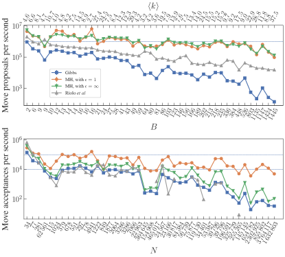
Figure 1: Number of single-node move proposals (top panel) and acceptances (bottom panel) per second, for several empirical networks gathered from the KONECT repository Kunegis (2013), with number of nodes $N$, average degree ${\left<k\right>}$ and occupied groups $B$ indicated in axis legends. The different curves correspond to the single-node moves described in the text, as well as the algorithm by Riolo et al Riolo et al. (2017), as shown in the legend. Missing points indicate a lack of recorded events in the allotted time. All algorithms were initialized with the same partition obtained with the agglomerative heuristic of Peixoto (2014a), and run for the same amount of time.

Although this kind of performance may seem encouraging at first, it is not difficult to see that ultimately this kind of approach cannot work very well. Consider, for example, starting the Markov chain from a partition consisting of a single group containing all the nodes. The only possible way forward is for one of the nodes to be placed on a different group on its own. However, for a majority of networks, such move will almost always be rejected. By means of a concrete example, consider the American football network of Ref. Girvan and Newman (2002), composed of 115 nodes and 613 edges, which has a clear community structure. For this network, starting from a single group partition, the easiest node to move to a new group needs to overcome a posterior probability ratio $\pi(\bm{b}^{\prime})/\pi(\bm{b})\approx 6.13\times 10^{-8}$. This means that such a move will be accepted for the first time, on average, only after around $10^{8}$ attempts, and even when this happens, the next accepted move is overwhelmingly more likely to be the one that puts this node back into its single group, moving the chain back to its initial state. The Markov chain, even though it is in theory ergodic, effectively behaves as if it were not, because it is forced to go through such states with very low probability, before reaching those that are more likely. It is clear from this example that the same problem can happen also when the starting state has more than one group, for example when two clear communities are merged into one: For these nodes to be split into two groups, this process must begin by placing one of the nodes into a new group by itself, which likewise will be almost always rejected. The same problem occurs also in the reverse direction: in order for an arbitrary division of a community into two groups to be merged into one, even if this final state has a much higher probability, it can only be reached by making one of the groups progressively smaller, until it is left with a single node, which is then finally vacated. Even though this last step is likely to be accepted, the ones preceding it are progressively less probable, and would almost never be observed in any practical amount of time.

Attempts to alleviate this effective lack of ergodicity include sophisticated heuristics for initialization of the Markov chain, such as the agglomerative approach of Ref. Peixoto (2014a), which tries to place the initial position of the chain closer to the most likely partitions, in the hope these low probability barriers will not be relevant there. However, this assumption can be easily violated in situations where posterior distribution ascribes high probabilities to partitions with different number of groups, and an efficient algorithm would need to visit them all. In the following, we address this limitation by allowing the chain to skip over these barriers by performing the merging and splitting of groups as a single step of the Markov chain.

III.2 Merges and splits

To overcome the limitations of single-node moves, we may introduce moves where entire groups are merged together. We implement this by selecting an existing group $r$ with a uniform probability $P(r)=1/B(\bm{b})$ and moving all its nodes to a different group $s$ with probability $P(s|r,\bm{b})$, yielding a transition proposal

$$P(\bm{b}^{\prime}|\bm{b})=\\ \sum_{rs}P(r)P(s|r,\bm{b})\left[\prod_{i}\left(\delta_{b_{i}^{\prime},s}\right)^{\delta_{b_{i},r}}\left(\delta_{b_{i}^{\prime},b_{i}}\right)^{1-\delta_{b_{i},r}}\right],$$ (17)

The simplest merge choice is one where the second group is chosen uniformly at random

$$P(s|r,\bm{b})=\frac{1-\delta_{rs}}{B(\bm{b})-1}.$$ (18)

However, we have already seen the suboptimal acceptance rate of such random choices when doing single-node moves, and we should expect the same problems to occur when doing merges as well. Following the same line as before, a smarter merge proposal is

$$P(s|r,\bm{b})=\frac{1-\delta_{sr}}{n_{r}}\sum_{i}\delta_{b_{i},r}\frac{P_{e}(s|i,\bm{b})}{1-P_{e}(r|i,\bm{b})},$$ (19)

where $P_{e}(s|i,\bm{b})$ is given by Eq. 14. This amounts to a uniformly random selection of a node in group $r$, and using it to perform the same smart selection of group $s$ as before, but ignoring the situation where $s=r$, and using that as a merge proposal.

Such merge proposals are straightforward to implement, but in order for this to incorporated into the MH scheme we need to be able to propose “split” moves that go in the reverse direction, i.e. we need to be able to select a subset of the nodes in group $r$ and move them to a new group $s$. We denote this subset via a binary vector ${\bm{x}}=\{0,1\}^{N}$, where $x_{i}=1$ if node $i$ is selected to move from group $r$ to $s$, otherwise $x_{i}=0$. This leads us to a move proposal that can be written as

$$P(\bm{b}^{\prime}|\bm{b})=\\ \sum_{r}P(r)\sum_{{\bm{x}}}P({\bm{x}}|r,\bm{b})\left[\prod_{i}\left(\delta_{b_{i}^{\prime},s(\bm{b})}\right)^{\delta_{x_{i},1}}\left(\delta_{b_{i}^{\prime},b_{i}}\right)^{\delta_{x_{i},0}}\right],$$ (20)

where $s(\bm{b})$ denotes the new group not currently occupied in partition $\bm{b}$ (we do not differentiate between unoccupied groups). A simple, but ultimately naive way of moving forward is to sample ${\bm{x}}$ in two stages: at first we select the number $m$ of nodes to be moved uniformly at random in the interval $[1,n_{r}-1]$ with probability

$$P(m|r,\bm{b})=\frac{1}{n_{r}-1},$$ (21)

and then sample the $m$ nodes uniformly at random, with a probability

$$P({\bm{x}}|r,\bm{b},m)=\frac{\delta_{m,\sum_{i}x_{i}}}{{n_{r}\choose m}},$$ (22)

yielding thus

$$P({\bm{x}}|r,\bm{b})=\sum_{m=1}^{n_{r}-1}P({\bm{x}}|r,\bm{b},m)P(m|r,\bm{b}).$$ (23)

Although this approach is easy to implement, it does not work in practice, because such fully random split proposals are almost never accepted, since the number of good splits, even when they exist, is exponentially outnumbered by bad ones. Furthermore, the above puts a low probability for every possible split, which means that it will also cause good merges to be rejected, as they cannot be easily reversed under this scheme.

At this point, it is important to realize that finding group splits is just a smaller scale version of our original problem of finding good overall partitions of the whole network, so we should not expect it be accomplished in one fell swoop. This inherent difficulty in proposing splits makes a merge-split MCMC less straightforward than one might realize at first. Although we might consider employing one of the many possible heuristics to find such good splits, we stumble upon two difficulties: 1. Besides sampling from it, we need also to be able to compute the probability of the proposal, to decide whether it can be accepted; 2. Given a merge proposal, we need to compute the corresponding split probability in the reverse direction, without actually sampling from the split proposal. These requirements limit the kind of schemes we have at our disposal. Luckily, as it has been shown before by Jain and Neal Jain and Neal (2004, 2007) in the context of Dirichlet process mixture models, we can overcome these limitations and perform splits with a much higher acceptance rate by making use of a split “staging” step as an auxiliary variable, as we describe in the following.

III.2.1 Auxiliary variables and split staging

Let us recall the detailed balance condition that needs to be fulfilled for the Markov chain to converge to the target distribution,

$$\pi(\bm{b})T(\bm{b}^{\prime}|\bm{b})=\pi(\bm{b}^{\prime})T(\bm{b}|\bm{b}^{\prime}),$$ (24)

where $T(\bm{b}^{\prime}|\bm{b})$ is the transition probability, after the rejection step has been considered. Now, let us consider an augmented version of the posterior distribution obtained by sampling an arbitrary auxiliary variable $\alpha$ with probability $P(\alpha|\bm{b})$. If we use MCMC to sample from the joint distribution $P(\alpha,\bm{b})=P(\alpha|\bm{b})\pi(\bm{b})$, then we can marginalize it to obtain the original distribution $\pi(\bm{b})=\sum_{\alpha}P(\alpha,\bm{b})$, therefore sampling from this augmented space subsumes sampling from the original one. The usefulness of introducing this auxiliary variable comes from the fact that we can use it to condition our move proposals, as we will see. The detailed balance condition in this case reads

$$P(\alpha|\bm{b})\pi(\bm{b})T(\alpha^{\prime},\bm{b}^{\prime}|\alpha,\bm{b})=P(\alpha^{\prime}|\bm{b}^{\prime})\pi(\bm{b}^{\prime})T(\alpha,\bm{b}|\alpha^{\prime},\bm{b}^{\prime}).$$ (25)

We can choose the joint transition by first making a transition $\bm{b}\to\bm{b}^{\prime}$ and then sampling the auxiliary variable from its conditional distribution, i.e.

$$T(\alpha^{\prime},\bm{b}^{\prime}|\alpha,\bm{b})=P(\alpha^{\prime}|\bm{b}^{\prime})T(\bm{b}^{\prime}|\alpha,\bm{b}),$$ (26)

Then the above detailed balance condition boils down to

$$\pi(\bm{b})T(\bm{b}^{\prime}|\bm{b},\alpha)=\pi(\bm{b}^{\prime})T(\bm{b}|\bm{b}^{\prime},\alpha^{\prime}),$$ (27)

which, importantly, is independent of the probability $P(\alpha|\bm{b})$. This condition is the same as the detailed balance for the original system, with the difference that the transitions are conditioned on arbitrary values of the auxiliary variable. We can incorporate this into the Metropolis-Hastings framework by conditioning our proposals $P(\bm{b}^{\prime}|\bm{b},\alpha)$, and accepting them with probability

$$\min\left(1,\frac{\pi(\bm{b}^{\prime})P(\bm{b}|\bm{b}^{\prime},\alpha^{\prime})}{\pi(\bm{b})P(\bm{b}^{\prime}|\bm{b},\alpha)}\right),$$ (28)

which will enforce the condition above. The key advantage here is that we do not need to know how to compute the probability $P(\alpha|\bm{b})$; we need only to be able to sample from this distribution. In other words, the transition probabilities themselves can be randomly sampled, without affecting detailed balance, and without requiring us to compute their probability. This gives us freedom to implement more elaborate schemes, and leads us to the notion of split staging, where as an auxiliary variable we use a tentative split $\hat{{\bm{x}}}$, which is again a binary vector with elements $\hat{x}_{i}\in\{0,1\}$, defined for the nodes that belong to the group being split, which is sampled from some arbitrary distribution (which we will discuss shortly), and we perform the final split via a single Gibbs sweep from that initial state, whose probability can be easily computed as

$$P({\bm{x}}|r,\bm{b},\hat{\bm{x}})=\prod_{i\in V_{r}}P(x_{i}|r,\bm{b},x_{1},\dots,x_{i-1},\hat{x}_{i+1},\dots,\hat{x}_{N}),$$ (29)

where $r$ is the group being split, $V_{r}$ is the set of nodes that belong to it, and

$$P(x_{i}|r,\bm{b},x_{1},\dots,x_{i-1},\hat{x}_{i+1},\dots,\hat{x}_{N})=\\ \frac{\pi\left(\bm{b}^{\prime}(x_{1},\dots,x_{i-1},x_{i},\hat{x}_{i+1},\dots,\hat{x}_{N})\right)}{\sum_{x=0}^{1}\pi\left(\bm{b}^{\prime}(x_{1},\dots,x_{i-1},x,\hat{x}_{i+1},\dots,\hat{x}_{N})\right)}$$ (30)

is the probability of moving node $i$ to either $x_{i}=0$ or $1$ in sequence, with the shortcut notation $\bm{b}^{\prime}({\bm{x}})=(b_{1}^{\prime}(x_{1}),\dots,b_{N}^{\prime}(x_{N}))$ given by

$$b_{i}^{\prime}(x_{i})=\begin{cases}s&\text{ if }x_{i}=1\text{ and }b_{i}=r,\\ b_{i}&\text{ otherwise. }\end{cases}$$ (31)

This yields a total split proposal probability

$$P(\bm{b}^{\prime}|\bm{b},\hat{\bm{x}})=\sum_{r}P(r)\sum_{{\bm{x}}}P({\bm{x}}|r,\bm{b},\hat{\bm{x}})\prod_{i}\delta_{b^{\prime}_{i},b_{i}^{\prime}(x_{i})},$$ (32)

which is conditioned on the stage split $\hat{\bm{x}}$, sampled from an arbitrary distribution. Note that this choice guarantees the strict reversibility of every possible merge since any split has a strict nonzero probability, regardless of the staging split $\hat{\bm{x}}$.

We need now only to determine how to sample the staging split $\hat{\bm{x}}$, but we can proceed in a variety of ways, since we do not need to compute the resulting probabilities. Here we can incorporate previous knowledge about what kind of heuristics work better for this problem. As was shown in Ref. Peixoto (2014a), starting from a random division, and then moving one node at a time, usually yields very bad performance, as this scheme needs a long time to find the optimal division. This happens even if the optimal division is very clear, with a very high posterior probability, since the initial random division effectively hides it from view, and the MCMC sampling essentially does a random walk in the configuration space, before it can find the best split. As an alternative, in Ref. Peixoto (2014a) it was shown that agglomerative schemes work significantly better, where one first puts each node in their own group, then proceeds by merging groups together, until the desired number of groups is reached. What typically happens in this scheme is that the intermediary partitions reached amount to subdivisions of the final partition, thus overcoming the entropic barriers seen by the random initial division scheme, and thus achieving the good split in a shorter time. However, we need also to consider a rather unintuitive property of the dual role of our split proposal, which functions also as a mechanism to reverse merge proposals. Suppose we are considering an “easy” merge of two groups that represent a very bad local division, i.e. if we had a chance to merge the groups and split them again, we would be able to find a much better division. In this situation, since our split proposal would suggest such a bad split only with a vanishingly small probability, this would also prevent us from merging the two groups, since the unlikely reversal would severely penalize the MH acceptance probability. However, if we also sometimes propose “bad” splits, then this would allow such merges to be accepted. Therefore, counterintuitively, what we need is a variety of split proposals, that are both good and bad Wang and Russell (2015). After experimentation, we determined that the following scheme, which combines a variety of strategies, works well in a majority of cases. We begin by sampling a prestaging split $\hat{\bm{x}}^{0}$ uniformly at random from one of the following three algorithms:

1. Random split:

   1. We sample the split size $m$ uniformly at random from the interval $[1,n_{r}-1]$.

   2. We choose $\hat{\bm{x}}^{0}$ uniformly at random from all splits of size $\sum_{i}\hat{x}_{i}^{0}=m$.

2. Sequential spreading:

   1. We move all nodes in group $r$ to an empty group $t$.

   2. In random order, we chose the nodes sequentially and move them either to group $r$ or group $s$, with probability proportional to $\pi(\hat{b}_{1},\dots,\hat{b}_{i},\dots,\hat{b}_{N})$ for a node $i$, with $\hat{\bm{b}}$ being the current working partition, except for the first two moves, which are to groups $r$ and $s$, to prevent leaving either group empty. In the end, to a node with $\hat{b}_{i}=r$ we set $\hat{x}_{i}^{0}=0$, and if $\hat{b}_{i}=s$, we set $\hat{x}_{i}^{0}=1$.

3. Sequential coalescence:

   1. We move each node $i$ in group $r$ to its own previously empty group $t_{i}$, which in the end all have a single node each.

   2. We proceed like 2(b) above.

From the prestage $\hat{\bm{x}}^{0}$, we obtain $\hat{\bm{x}}$ by performing $M$ sequential Gibbs sweeps for every node in group $r$ and $s$, where they are allowed to move only between these two groups, forbidding moves that would leave either group empty. Note that although we could in principle compute the probability of proposing the premerge step, this becomes intractable after the Gibbs sweeps are performed, since we would need to compute the probability of reaching the final state via every possible intermediate trajectory. But this is precisely what is not needed in this scheme.

With the stage split in place, the final proposal is obtained by performing one more Gibbs sweep as described previously, and it is then accepted with probability

$$\min\left(1,\frac{\pi(\bm{b}^{\prime})P(\bm{b}|\bm{b}^{\prime})}{\pi(\bm{b})P(\bm{b}^{\prime}|\bm{b},\hat{\bm{x}})}\right),$$ (33)

where the reverse transition $P(\bm{b}|\bm{b}^{\prime})$ corresponds to a merge proposal. Likewise a merge can be accepted with probability

$$\min\left(1,\frac{\pi(\bm{b}^{\prime})P(\bm{b}|\bm{b}^{\prime},\hat{\bm{x}})}{\pi(\bm{b})P(\bm{b}^{\prime}|\bm{b})}\right),$$ (34)

which means we always need to generate a staging split $\hat{\bm{x}}$ for each merge candidate, using the algorithm above, to compute the reverse proposal probability.

As the number $M$ of Gibbs sweeps made during the staging step increases, the more likely it becomes that the split will be proposed with a probability proportional to the target distribution $\pi(\bm{b})$, which would be optimal. In practice, however, we do not want to choose this value too large, as it is not worth to spend too much time in a single Monte Carlo step. Although the optimal value is likely to vary for each network, we found that a value around $M=10$ offers a good trade-off between speed and proposal quality in most experiments we made.

III.2.2 Joint merge-split moves

We also consider an additional kind of move that keeps the number of groups constant, and is composed of a merge of group $r$ into $s$, which is then split again by moving some nodes from $s$ to back to $r$, following the same scheme as before. This amounts to a proposal probability

$$P(\bm{b}^{\prime}|\bm{b},\hat{\bm{x}})=\\ \sum_{rs}P(r)P(s|r,\bm{b})\sum_{\hat{\bm{b}}}\left[\prod_{i}\left(\delta_{\hat{b}_{i},s}\right)^{\delta_{b_{i},r}}\left(\delta_{\hat{b}_{i},b_{i}}\right)^{1-\delta_{b_{i},r}}\right]\times\\ \sum_{{\bm{x}}}P({\bm{x}}|s,\hat{\bm{b}},\hat{\bm{x}})\prod_{i}\delta_{b_{i}^{\prime}(x_{i}),b_{i}^{\prime}},$$ (35)

and the final move is accepted with probability

$$\min\left(1,\frac{\pi(\bm{b}^{\prime})P(\bm{b}|\bm{b}^{\prime},\hat{\bm{x}}^{\prime})}{\pi(\bm{b})P(\bm{b}^{\prime}|\bm{b},\hat{\bm{x}})}\right).$$ (36)

This kind of move is able to re-distribute the nodes between two groups, without going through states with a smaller or lower number of groups, which we found to improve mixing in circumstances where the number of groups tends not to vary significantly in the posterior distribution.

III.3 Algorithm overview and overall complexity

Even though the split and merge moves are strictly sufficient to guarantee ergodicity and detailed balance, the mixing time of the Markov chain is improved if we combine all types of moves considered above. We do so by introducing the relative move propensities $\omega_{\text{single}}$, $\omega_{\text{merge}}$, $\omega_{\text{split}}$ and $\omega_{\text{merge-split}}$, such that, e.g. the probability of a single-node move is given by

$$\frac{\omega_{\text{single}}}{\omega_{\text{single}}+\omega_{\text{merge}}+\omega_{\text{split}}+\omega_{\text{merge-split}}},$$ (37)

and likewise for the other kinds of moves. At each step we choose one of the moves above with the corresponding probability, and accept or reject according to the appropriate MH criterion. We note that for merge and splits we need to incorporate these move probabilities into the rejection criterion, e.g. for merge proposals we have

$$\min\left(1,\frac{\pi(\bm{b}^{\prime})P(\bm{b}|\bm{b}^{\prime},\hat{\bm{x}})\,\omega_{\text{split}}}{\pi(\bm{b})P(\bm{b}^{\prime}|\bm{b})\,\omega_{\text{merge}}}\right),$$ (38)

and likewise for splits. In our experiments, we found it more efficient to propose single nodes more often, and we have chosen $\omega_{\text{single}}=N$ and $\omega_{\text{merge}}=\omega_{\text{split}}=\omega_{\text{merge-split}}=1$ for our analysis. It is also possible to determine optimal choices for these parameters by performing preliminary runs of the algorithm, and then choosing the values according to the observed acceptance rates.

In summary, the overall structure of the algorithm is as follows:

1. At each step, we choose to perform either a single-node, merge, split or merge-split move according to Eq. 37 or the analogous for the other moves.

2. For single node moves, we make a move proposal according to Eqs. 12 and 15, and we accept it according to the MH criterion.

3. For merges, we make a proposal according to Eqs. 17 and  19, and accept it with the MH criterion of Eq. 38, which involves computing the move reversal probability via a split, which is obtained according to Eq. 32, conditioned on a sampled staged split. The staged split is sampled in the same manner as when performing split proposals.

4. For splits, we make a proposal according to Eq. 32, which involves performing a prestage split using either the random, sequential spreading or sequential coalescence strategies, chosen uniformly at random, followed by $M$ Gibbs sweeps to obtain the staged split. From that, we perform the final split proposal via a single Gibbs sweep. We accept it according to the equivalent MH criterion of Eq. 38, which involves computing the reverse merge proposal probability, according to Eq. 17

5. For merge-splits, we make a proposal according to Eq. 35, which involves performing both a merge and a split, and accept it according to Eq. 36, which involves a merge-split that reverses it.

If the model parametrization of Ref. Peixoto (2017) is used, the move of a single node $i$ to another group can be done in time $O(k_{i})$, where $k_{i}$ is its degree. Because of this, the time taken to perform a split of group $r$ is $O[M(n_{r}+e_{r})]$, where $M$ is the number of Gibbs sweeps used in the split staging, $e_{r}=\sum_{i}k_{i}\delta_{b_{i},r}$ and we need to process every node even if they have zero degree. Likewise, to merge group $r$ with $s$ we need time $O(n_{r}+e_{r})$, but since we need to compute the reverse split proposal to obtain the acceptance probability, we need in fact time $O[M(n_{r}+n_{s}+e_{r}+e_{s})]$. Since the different move proposals involve a different number of nodes, their relative probabilities will determine the typical running time. The longest a merge, split or merge-split move can take is $O[M(N+E)]$, and hence choosing single-node moves more often with $\omega_{\text{single}}=O[M(N+E)\times\max(\omega_{\text{merge}},\omega_{\text{split}},\omega_{\text{merge-split}})]$ means that an entire sweep of $N$ move proposals can be done in expected linear time $O(N+E)$. A C++ implementation of the algorithm is freely available as part of the graph-tool Python library Peixoto (2014c).

IV Performance for empirical networks

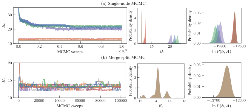
Figure 2: Comparison of runs with the single-node and merge-split MCMC algorithms, for a network of friendships between $N=678$ high school students Moody (2001), starting for $B=N$ and $B=1$ states (except for the single-node algorithm, where the $B=1$ initialization is replaced with an agglomerative heuristic) showing the values of the effective number of groups $B_{e}$ as a function of the number of sweeps (where one sweep equals $N$ move proposals), the resulting distribution of $B_{e}$ values and unnormalized posterior probability $P(\bm{b},\bm{A})$ for each run, drawn with different colors.

In Fig. 2 we show a comparison between the single-node and merge-split MCMC algorithms for a network of friendships between $N=678$ high school students Moody (2001). We compare six runs of each algorithm, half of which start from the $B=N$ single-node groups state, and the other half from the single-group $B=1$ state, except for the single-node MCMC runs which would get trivially trapped in this state, in which case we initialize from an estimate of the ground state using the agglomerative heuristic described in Ref. Peixoto (2014a). To analyze the convergence of the chain, we compute the effective number of groups $B_{e}=\mathrm{e}^{S}$, where

$$S=-\sum_{r}\frac{n_{r}}{N}\ln\frac{n_{r}}{N},$$ (39)

is the entropy of the group membership distribution. As the results show, the single-node algorithm fails to equilibrate the chain even after an inordinate number of $10^{9}$ sweeps, as the different starting states do not converge to the same values. The initial states with a large number of groups remain at a relatively larger value, due the “merge” barriers we have described previously. More worryingly, even the improved starting states fail to make the algorithm work, as the chains clearly remain trapped in different sets of partitions. It is important to note that individual chains do not show any sign of a lack of equilibration, as they are seemingly trapped in metastable states, but they completely fail to accurately represent the target distribution. It is only when we compare different runs of the algorithm that we see a problem.

The merge-split MCMC, however, yields a substantially improved performance, where the diverging starting states converge only after a few sweeps to the same set of sampled states. The posterior distribution of effective number of groups $B_{e}$ and unnormalized posterior probability $P(\bm{b},\bm{A})$ are identical between the different runs, serving as strong evidence for their successful equilibration. The pronounced multiple peaks in the $B_{e}$ distribution represent the multimodality of the posterior distribution that the single-node version of the algorithm cannot overcome.

The single-node algorithm can in fact work for networks which are sufficiently small. For example, if we apply it to the co-appearance network of $N=77$ characters of the novel Les Misérables by Victor Hugo Knuth (1993), then we obtain essentially the same performance with both algorithms, as shown in Fig. 3. We can measure in more detail the mixing time of the Markov chain by computing the autocorrelation of a surrogate statistics, for example for $B_{e}$ we have

$$\rho(\tau)=\frac{\sum_{t}[B_{e}(t)-{\left<B_{e}\right>}][B_{e}(t+\tau)-{\left<B_{e}\right>}]}{\sum_{t}[B_{e}(t)-{\left<B_{e}\right>}]^{2}},$$ (40)

where $B_{e}(t)$ is the value of $B_{e}$ after $t$ steps of the Markov chain, and ${\left<B_{e}\right>}$ is the mean value in the whole range. The value of $\tau$ for which $\rho(\tau)$ approaches zero gives the decorrelation time after which we expect samples to be independent (provided the chain is not trapped in a metastable state). As seen in Fig. 3, the merge-split algorithm de-correlates faster, but the difference is very small in this example.

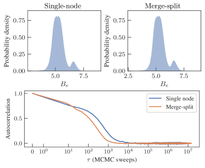
Figure 3: Posterior distribution of the effective number of groups $B_{e}$ obtained with the single-node and merge-split algorithms (top panel), as well as the respective autocorrelation functions (bottom panel), for the co-appearance network of $N=77$ characters of the novel Les Misérables by Victor Hugo Knuth (1993).

	Single-node		Merge-split
Network	$n$	ESS	$n$	ESS
Les Misérables	5,216,662	1,026,851	2,984,113	2,494,560
Football	13,036,736	2,532∗	5,490,028	190,267
High school	9,907,093	7∗	2,457,300	9,945

Table 1: Number of MCMC samples $n$ and effective sample size (ESS) obtained with the single-node and merge-split MCMC algorithms, for three empirical networks, as described in the text. Values marked with $*$ correspond to runs that failed to equilibrate even after a long time, and hence the ESS values should not be trusted.

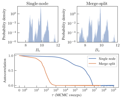
Figure 4: Posterior distribution of the effective number of groups $B_{e}$ obtained with the single-node and merge-split algorithms (top panel), as well as the respective autocorrelation functions (bottom panel), for the network of American football games between $N=115$ teams Girvan and Newman (2002).

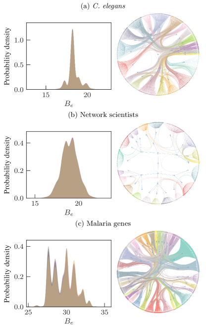
Figure 5: Distribution of the effective number of groups $B_{e}$ at the lowest hierarchical level, obtained for several merge-split MCMC runs, starting from different initial conditions (with $B=1$, $B=N$ and an approximation of the ground state) drawn with different colors (left) and corresponding marginal hierarchical partition (right), for the neural network the C. elegans organism White et al. (1986), the co-authorship network of network scientists Newman (2006), and the network of recombinant antigen genes from the human malaria parasite P. falciparum Larremore et al. (2013). In all cases, the different distributions coincide, indicating convergence to the target distribution.

A related quantity that is useful to determine the actual performance of the MCMC is the effective sample size (ESS) defined as

$$\text{ESS}=\frac{n}{1+\frac{1}{2}\sum_{\tau=1}^{\infty}\rho(\tau)},$$ (41)

where $n$ is the total number of samples taken from the MCMC run, and $\rho(\tau)$ is the autocorrelation computed over only those samples. The ESS is interpreted as the effective number of uncorrelated samples taken during the run of the algorithm (provided it has equilibrated). If the chain is ideal, then we should have $\text{ESS}(n)\approx n$, but this is often not the case. In Table 1 we show the number of samples and the ESS values for the three networks considered previously, where the samples were gathered after several MCMC sweeps. For the Les Misérables network, the ESS with the merge-split algorithm is close to ideal, although the single-node version is still quite usable. For both the high school and football networks we see a large difference in the usefulness of both algorithms. In fact, we had already seen that for the high school network the single-node MCMC simply fails to converge, meaning that the actual ESS for that case should be in fact zero. For the football network we see in Fig. 4 the autocorrelation obtained with both algorithms, as well as the posterior $B_{e}$ distribution. Not only is the decorrelation four orders of magnitude slower with the single-node algorithm, but also it in fact fails to correctly sample from all modes of the distribution, omitting values in the range $B_{e}\in[7,8]$, even though they do not have a negligible posterior probability. Therefore, even though this network is not very large, a detailed sampling from the posterior distribution using the single-node algorithm is already quite demanding. For network sizes that are slightly larger, such as the high school network, it breaks down completely, leaving the merge-split version as the only viable alternative.

V Hierarchical partitions

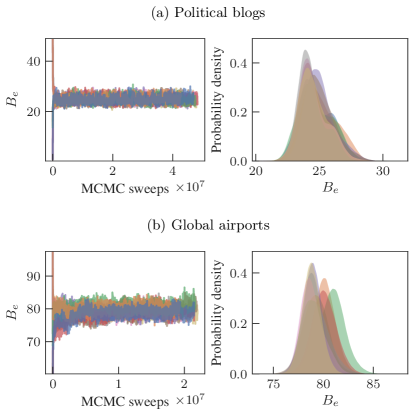
Figure 6: Effective number of groups $B_{e}$ at the lowest level during several long runs of the merge-split MCMC algorithm using the hierarchical SBM, drawn with different colors, and corresponding distribution, for a network of political blogs Adamic and Glance (2005) and flights between airports from https://openflights.org. In this case, discrepancies between the different distributions are still noticeable after long runs, indicating a lack of convergence to the target distribution.

The nested SBM Peixoto (2014b, 2017) consists of a hierarchical Bayesian model, where the parameters of the SBM are interpreted as a multigraph, which are then sampled from another SBM, and so on recursively, forming a nested hierarchy. The nodes at level $l+1$ are the (nonempty) group labels at level $l$, and we have a set of partitions $\{\bm{b}_{1},\dots,\bm{b}_{L}\}$, sampled from the posterior distribution

$$P(\bm{b}_{1},\dots,\bm{b}_{L}|\bm{A})=\frac{P(\bm{A}|\bm{b}_{1},\dots,\bm{b}_{L})P(\bm{b}_{1},\dots,\bm{b}_{L})}{P(\bm{A})},$$ (42)

where

$$P(\bm{A}|\bm{b}_{1},\dots,\bm{b}_{L})P(\bm{b}_{1},\dots,\bm{b}_{L})\\ =P(\bm{A}|\bm{e}_{1},\bm{b}_{1})\prod_{l=1}^{L}P(\bm{e}_{l}|\bm{e}_{l+1},\bm{b}_{l+1})P(\bm{b}_{l}|\bm{b}_{l-1}),$$ (43)

is the marginal likelihood (we refer to Ref. Peixoto (2017) for more details).

For this model, we can employ the same MCMC described above, by sampling from the conditional posterior distribution at each hierarchy level $l$,

$$P(\bm{b}_{l}|\bm{b}_{1},\dots,\bm{b}_{l-1},\bm{b}_{l+1},\dots,\bm{b}_{L},\bm{A})\\ \begin{aligned} &=\frac{P(\bm{b}_{1},\dots,\bm{b}_{L}|\bm{A})}{\sum_{\bm{b}^{\prime}_{l}}P(\bm{b}_{1},\dots,\bm{b}^{\prime}_{l},\dots,\bm{b}_{L}|\bm{A})}.\end{aligned}$$ (44)

This means we can proceed at each step in the MCMC by choosing a level $l$ uniformly at random, and setting $\pi(\bm{b}_{l})=P(\bm{b}_{l}|\bm{b}_{1},\dots,\bm{b}_{l-1},\bm{b}_{l+1},\dots,\bm{b}_{L},\bm{A})$ as our target distribution, and making move proposals the exact same way as before, by performing either a single-node, merge, split, or merge-split move. The only special consideration needed is when a new group is added at a given level, a node needs to be added to the level above, together with its group membership, and possibly so on recursively. This kind of new group addition needs to be able to reverse the disappearance of a group, together with its node at the next level, and so on. The way we proceed is to keep track of unoccupied groups and their own nodes in the hierarchy, even though they do not contribute to the posterior probability, with the only purpose of being able to reverse group vacancies and to propose placement of new groups. This bookkeeping needs only to be virtual, since at any given time an unoccupied group can belong to either one of the $B$ occupied groups at the level above or an unoccupied one, with equal probability. Therefore, whenever a new group is occupied, its own group membership at level $l$ is chosen uniformly at random with probability

$$\frac{1}{B(\bm{b}_{l})+1},$$ (45)

and so on recursively for the higher levels if a new group is chosen.

In Fig. 5 we see the above algorithm employed to sample from the hierarchical partitions of a few empirical networks, in particular the neural network the C. elegans organism White et al. (1986), the co-authorship network of network scientists Newman (2006), and the network of recombinant antigen genes from the human malaria parasite P. falciparum Larremore et al. (2013). For these results we considered several chains, where the lowest level of the hierarchy was initialized both at $B=1$ and $B=N$, and in all cases they converged to the same overall distribution of hierarchical partitions.

The convincing equilibration results we observe for the examples above are not universal, and for some data the merge-split algorithm is seemingly not sufficient to fully equilibrate the chain, at least not in a short amount of time. Some examples of this are shown in Fig. 6 for a network of $N=1,222$ political blogs Adamic and Glance (2005) and flights between $N=3,286$ airports from https://openflights.org. Although the scheme succeeds in quickly converging to the same range of partitions, with no obvious memory of the starting state, the values sampled still show noticeable discrepancy between the runs, even after a long time. This long equilibration time is not related to the hierarchical model, and also occurs when using the “flat” model for these examples. The behavior in this case seems different from the metastable trapping observed with the single-node scheme, and is probably due to a different kind of multimodality that the merge and splits are not able to efficiently evade. This behavior is likely to be an indication of a bad quality of fit of the SBM for these networks, and requires a strategy different from the merging and splitting of groups to be effectively addressed.

VI Conclusion

We have showed how merge and split moves can be introduced into MCMC schemes that sample network partitions from a posterior distribution, thereby significantly improving the mixing time of the Markov chain in a variety of empirically relevant scenarios. We have also demonstrated how the often employed approach of moving the group membership of a single node at a time is systematically insufficient to characterize the posterior distribution of group assignments, due to its tendency of getting trapped in metastable states.

We have extended the algorithm also to the case of hierarchical partitions, allowing us to sample nested hierarchical clusterings with the same degree of efficiency. The method developed does not depend on details of the underlying model, and can be easily extended to other variations as well.

When investigating the performance of the merge-split scheme in a variety of empirical networks we also encountered situations where, although it is far less susceptible to getting trapped as the single node scheme, it may still need very long runs to sufficiently explore the posterior landscape of partitions. A better understanding of the reasons behind the sampling difficulty in these cases may prove important to a full characterization of the modular network structure in empirical settings, and in particular to determine the quality of fit of network models used for community detection. The latter is because this kind of roughness of the posterior distribution is not expected if the network is truly sampled from the assumed generative model, and may point to a unsuitability of the model for that particular data. We leave this line of inquiry for future work.

References

- Fortunato (2010) Santo Fortunato, “Community detection in graphs,” Physics Reports 486, 75–174 (2010).
- Peixoto (2019a) Tiago P. Peixoto, “Bayesian Stochastic Blockmodeling,” in Advances in Network Clustering and Blockmodeling (John Wiley & Sons, Ltd, 2019) pp. 289–332.
- Guimerà et al. (2004) Roger Guimerà, Marta Sales-Pardo, and Luís A. Nunes Amaral, “Modularity from fluctuations in random graphs and complex networks,” Physical Review E 70, 025101 (2004).
- Bagrow (2012) James P. Bagrow, “Communities and bottlenecks: Trees and treelike networks have high modularity,” Physical Review E 85, 066118 (2012).
- Fortunato and Barthélemy (2007) Santo Fortunato and Marc Barthélemy, “Resolution limit in community detection,” Proceedings of the National Academy of Sciences 104, 36–41 (2007).
- Holland et al. (1983) Paul W. Holland, Kathryn Blackmond Laskey, and Samuel Leinhardt, “Stochastic blockmodels: First steps,” Social Networks 5, 109–137 (1983).
- Karrer and Newman (2011) Brian Karrer and M. E. J. Newman, “Stochastic blockmodels and community structure in networks,” Physical Review E 83, 016107 (2011).
- Decelle et al. (2011) Aurelien Decelle, Florent Krzakala, Cristopher Moore, and Lenka Zdeborová, “Asymptotic analysis of the stochastic block model for modular networks and its algorithmic applications,” Physical Review E 84, 066106 (2011).
- Snijders and Nowicki (1997) Tom A. B. Snijders and Krzysztof Nowicki, “Estimation and Prediction for Stochastic Blockmodels for Graphs with Latent Block Structure,” Journal of Classification 14, 75–100 (1997).
- Guimerà and Sales-Pardo (2009) Roger Guimerà and Marta Sales-Pardo, “Missing and spurious interactions and the reconstruction of complex networks,” Proceedings of the National Academy of Sciences 106, 22073 –22078 (2009).
- Peixoto (2014a) Tiago P. Peixoto, “Efficient Monte Carlo and greedy heuristic for the inference of stochastic block models,” Physical Review E 89, 012804 (2014a).
- Newman and Reinert (2016) M. E. J. Newman and Gesine Reinert, “Estimating the Number of Communities in a Network,” Physical Review Letters 117, 078301 (2016).
- Riolo et al. (2017) Maria A. Riolo, George T. Cantwell, Gesine Reinert, and M. E. J. Newman, “Efficient method for estimating the number of communities in a network,” Physical Review E 96, 032310 (2017).
- Peixoto (2017) Tiago P. Peixoto, “Nonparametric Bayesian inference of the microcanonical stochastic block model,” Physical Review E 95, 012317 (2017).
- Peixoto (2014b) Tiago P. Peixoto, “Hierarchical Block Structures and High-Resolution Model Selection in Large Networks,” Physical Review X 4, 011047 (2014b).
- Peixoto (2018a) Tiago P. Peixoto, “Nonparametric weighted stochastic block models,” Physical Review E 97, 012306 (2018a).
- Peixoto (2018b) Tiago P. Peixoto, “Reconstructing Networks with Unknown and Heterogeneous Errors,” Physical Review X 8, 041011 (2018b).
- Peixoto (2019b) Tiago P. Peixoto, “Network Reconstruction and Community Detection from Dynamics,” Physical Review Letters 123, 128301 (2019b).
- Peixoto (2020) Tiago P. Peixoto, “Latent Poisson models for networks with heterogeneous density,” arXiv:2002.07803 [physics, stat] (2020), arXiv: 2002.07803.
- Metropolis et al. (1953) Nicholas Metropolis, Arianna W. Rosenbluth, Marshall N. Rosenbluth, Augusta H. Teller, and Edward Teller, “Equation of State Calculations by Fast Computing Machines,” The Journal of Chemical Physics 21, 1087 (1953).
- Hastings (1970) W. K. Hastings, “Monte Carlo sampling methods using Markov chains and their applications,” Biometrika 57, 97 –109 (1970).
- Kunegis (2013) Jérôme Kunegis, “KONECT: The Koblenz Network Collection,” in Proceedings of the 22Nd International Conference on World Wide Web, WWW ’13 Companion (ACM, New York, NY, USA, 2013) pp. 1343–1350.
- Peixoto (2014c) Tiago P. Peixoto, “The graph-tool python library,” figshare (2014c), 10.6084/m9.figshare.1164194, available at https://graph-tool.skewed.de.
- Girvan and Newman (2002) M. Girvan and M. E. J. Newman, “Community structure in social and biological networks,” Proceedings of the National Academy of Sciences 99, 7821 –7826 (2002).
- Jain and Neal (2004) Sonia Jain and Radford M. Neal, “A Split-Merge Markov chain Monte Carlo Procedure for the Dirichlet Process Mixture Model,” Journal of Computational and Graphical Statistics 13, 158–182 (2004).
- Jain and Neal (2007) Sonia Jain and Radford M. Neal, “Splitting and merging components of a nonconjugate Dirichlet process mixture model,” Bayesian Analysis 2, 445–472 (2007).
- Wang and Russell (2015) Wei Wang and Stuart Russell, “A smart-dumb/dumb-smart algorithm for efficient split-merge MCMC,” (AUAI Press, 2015) pp. 902–911.
- Moody (2001) James Moody, “Peer influence groups: identifying dense clusters in large networks,” Social Networks 23, 261–283 (2001).
- Knuth (1993) Donald E. Knuth, The Stanford GraphBase: A Platform for Combinatorial Computing, 1st ed. (Addison-Wesley Professional, New York, N.Y. : Reading, Mass, 1993).
- White et al. (1986) J. G. White, E. Southgate, J. N. Thomson, and S. Brenner, “The structure of the nervous system of the nematode Caenorhabditis elegans,” Philosophical Transactions of the Royal Society of London. Series B, Biological Sciences 314, 1–340 (1986).
- Newman (2006) M. E. J. Newman, “Finding community structure in networks using the eigenvectors of matrices,” Physical Review E 74, 036104 (2006).
- Larremore et al. (2013) Daniel B. Larremore, Aaron Clauset, and Caroline O. Buckee, “A Network Approach to Analyzing Highly Recombinant Malaria Parasite Genes,” PLOS Comput Biol 9, e1003268 (2013).
- Adamic and Glance (2005) Lada A. Adamic and Natalie Glance, “The political blogosphere and the 2004 U.S. election: divided they blog,” in Proceedings of the 3rd international workshop on Link discovery, LinkKDD ’05 (ACM, New York, NY, USA, 2005) pp. 36–43.