Probing the singlet-triplet splitting in double quantum dots:
implications of the ac field amplitude

Abstract

We consider a double quantum dot whose energy detuning is controlled by an ac electric field. We demonstrate an energy configuration for which the ac-induced current flowing through the double dot directly probes the spin-orbit anticrossing point for small ac field amplitudes. On the contrary, as the ac amplitude increases a current antiresonance is formed, and the direct information about the spin-orbit interaction is lost. This result indicates that a large ac amplitude is not necessarily advantageous for the spectroscopy of spin-orbit coupled two-spin states. Moreover, we investigate the ac-induced current peaks versus the ac amplitude and show a current suppression when the ac field forms spin blocked states. This effect gives rise to a characteristic pattern for the current which can be controlled at will by tuning the ac amplitude. Our results can be explored by performing electronic transport measurements in the spin blockade regime.

I Introduction

Various spin qubit proposals in semiconductor materials make use of electron spins trapped in quantum dot systems. hanson07 ; zwanenburg13 Spin-orbit coupled spins defined in double dots at a constant magnetic field, can be manipulated electrically using an ac electric field. perge12 ; ono17 One clear signature of the spin-orbit interaction (SOI) is the formation of singlet-triplet anticrossing points in the two-electron energy spectrum. The magnitude of the energy gap at the anticrossing point is an important energy scale because it gives information about the strength and the direction of the SOI. anticros1 ; anticros2 ; nowak ; takahashi ; kanai ; stano ; fasth Usually a large gap is the result of strong SOI. Transport spectroscopy of the two-electron energy spectrum can be performed by measuring the electrical current through the double dot in the presence of an ac electric field. perge12 ; ono17 Current peaks arise when the appropriate resonant condition is satisfied, giavaras19 and information about the SOI can be extracted provided the ac-induced current peaks are well-formed in the vicinity of the SOI anticrossing point.

The applied ac field is characterized by the ac frequency and amplitude. The range of the ac frequency is dictated by the energy configuration of the two-electron eigenstates in the double dot and the relevant energy splitting. Therefore, the ac-induced peaks can be controlled by the ac amplitude only, provided the ac amplitude can be tuned by the applied voltages to gate electrodes.

In this work, we consider a double dot (DD) in the spin blockade regime, ono00 and focus on experimentally accessible DD energy configurations, where singlet and triplet energy levels anticross. In particular, the focus is on two SOI-coupled singlet-triplet states forming an anticrossing point, and a third state with triplet character. We assume that an ac field periodically changes the energy detuning of the DD, in the same way as in the experiments, perge12 ; ono17 and investigate possible implications of the magnitude of the ac amplitude in the ac-induced current peaks. We show that the current peaks allow for transport spectroscopy of the SOI anticrossing point only in a specific ac amplitude range, which is related to the strength of the SOI. When the ac amplitude is large the energy gap of the anticrossing can no longer be probed accurately, and instead an “antiresonance” is formed, where typically the ac current is suppressed. As a consequence, a large ac amplitude is not necessarily advantageous for spectroscopy, especially when the presence of the SOI is directly inferred by the current characteristics versus the ac frequency and magnetic field. Furthermore, we study the dependence of the ac-induced current on the energy detuning as well as the ac field amplitude, and identify a rather general pattern of high- and low-current regions. These regions stem from the formation of ac-induced spin blocked states, and thus can be controlled at will by tuning the ac amplitude.

In the next section, the double quantum dot model and the electronic transport model are presented. In Sec. III the ac-induced transport characteristics for different ac field frequencies and amplitudes are studied. The basic conclusions of this work are summarized in Sec. IV.

II Physical model

II.1 Double dot Hamiltonian

In this work, we consider two serially tunnel-coupled quantum dots in the spin blockade regime ono00 , and assume the dot charging energy to be much larger than the inter-dot tunnel coupling. The quantum dot 1 (dot 2) is coupled to the left (right) metallic lead, therefore under an appropriate bias voltage current can flow through the system which is sensitive to spin correlations. We assume that each dot is characterised by a single orbital level (on-site energy), and dot 2 is lower in energy so that a single spin is localised in dot 2, and the spin blockade regime can be realised. hanson07 ; zwanenburg13 ; ono00 In this regime the electronic transport through the DD system follows the charge cycle hanson07 ; zwanenburg13 ; ono00 : $(0,1)\rightarrow(1,1)\rightarrow(0,2)\rightarrow(0,1)$, where the notation $(n,m)$ indicates $n$ electrons on dot 1 and $m$ electrons on dot 2. The relevant two-electron states are the (1, 1) triplet states $|T_{+}\rangle$, $|T_{-}\rangle$, $|T_{0}\rangle$, the (1, 1) singlet state $|S_{11}\rangle$, and the (0, 2) singlet state $|S_{02}\rangle$. The (2, 0) singlet state $|S_{20}\rangle$ is much higher in energy and to a very good approximation, can be ignored without affecting the physics. hanson07 ; zwanenburg13

In the Appendix, we show that for two electrons and in the basis $|S_{11}\rangle$, $|T_{+}\rangle$, $|S_{02}\rangle$, $|T_{-}\rangle$, $|T_{0}\rangle$ the DD Hamiltonian is

$$H_{\mathrm{DD}}=\left(\begin{array}[]{ccccc}0&0&-\sqrt{2}t_{\mathrm{c}}&0&\Delta^{-}\\ 0&-\Delta^{+}&-t_{\mathrm{so}}&0&0\\ -\sqrt{2}t_{\mathrm{c}}&-t_{\mathrm{so}}&\delta&-t_{\mathrm{so}}&0\\ 0&0&-t_{\mathrm{so}}&\Delta^{+}&0\\ \Delta^{-}&0&0&0&0\\ \end{array}\right).$$ (1)

The Zeeman term on dot $i$ ($i=1$, 2) is given by $\Delta_{i}=g_{i}\mu_{\mathrm{B}}B$, where $B$ is the external magnetic field and $g_{i}$ is the $g$-factor with $\Delta^{\pm}=(\Delta_{1}\pm\Delta_{2})/2$. The parameter $t_{\mathrm{c}}$ is the inter-dot tunnel coupling which conserves spin, $t_{\mathrm{so}}$ is the spin-flip tunnel coupling due to the SOI, and $\delta$ is the energy detuning. Some experimental studies perge12 ; ono17 ; wang ; chorley11 on double quantum dots conclude that for the tunnel couplings $t_{\mathrm{so}}<t_{\mathrm{c}}$, and in this work we satisfy this condition. The one-electron states (0, 1) consist of the spin-up $|0,\uparrow\rangle$, and spin-down $|0,\downarrow\rangle$ configurations which are Zeeman-split due to the magnetic field $B$. The one-electron states (1, 0) can usually be ignored in the spin blockade regime provided the dots are weakly coupled. hanson07 ; zwanenburg13

We assume that an ac electric field periodically modulates the on-site orbital energy of dot 2, relative to dot 1. In this case, we can consider the energy of the (1, 1) states to be unaffected by the ac field, and the energy of the (0, 2) state to be time dependent. Thus, according to Hamiltonian Eq. (1) the energy detuning in this work is considered to be time periodic

$$\delta(t)=-\varepsilon+A\cos(2\pi ft),$$ (2)

where $A$, $f$ are the amplitude and frequency of the ac field respectively. In semiconductor quantum dots the value of $\varepsilon$ is controlled by applying appropriate gate voltages  hanson07 ; zwanenburg13 ; bertrand and the values of $A$, $f$ are tunable by electrical pulses. perge12 ; ono17 ; bertrand ; pulses1

For all the calculations the inter-dot tunnel coupling is taken to be $t_{\mathrm{c}}=13$ $\mu$eV, in agreement with experimentally reported values. hanson07 ; zwanenburg13 The $g$-factors of the two dots are taken to be $g_{1}=7$, and $g_{2}=7.5$. These absolute values are within the range of the $g$-factors reported for InAs systems. smith87 The $g$-factor difference of about 8$\%$ is consistent with that found in double quantum dots, and could be the result of the SOI, and/or the asymmetric double dot confining potential. Even larger $g$-factor differences have been reported. For instance, in Ref. berg, the absolute $g$-factor difference in an InSb double quantum dot with strong SOI was measured to be as large as 12; e.g. over 20$\%$ difference.

Figure 1: The upper frame shows the two-electron eigenenergies as a function of magnetic field. The two vertical arrows indicate possible transitions that can be induced by the ac electric field, which periodically changes the energy detuning of the double quantum dot. The lower frame shows the energy splitting $E_{5}-E_{1}$ and $E_{5}-E_{2}$ as a function of magnetic field.

The eigenstates of the DD Hamiltonian $H_{\mathrm{DD}}$ for $A=0$, are denoted by $|\psi_{n}\rangle$, $n=1$, 2,…5, and are ordered in increasing eigenenergy. We refer to $|\psi_{n}\rangle$ as singlet or triplet states, though $|\psi_{n}\rangle$ consist of both singlet and triplet components due to the SOI and the $g$-factor difference in the two dots. Thus, the spin blockade can be lifted and the ac field can induce singlet-triplet transitions. The corresponding DD eigenenergies $E_{n}$, $n=1$, 2,…5, versus the magnetic field are shown in the upper frame of Fig. 1, for $t_{\mathrm{so}}=1.5$ $\mu$eV and $\varepsilon=50$ $\mu$eV. In this work, we are interested in the region of the SOI induced anticrossing point which is formed at $B\approx 0.134$ T, and the corresponding gap is about 0.7 GHz. The ac field induced transitions of interest are between the state $|\psi_{5}\rangle$ which has triplet character, and the two SOI-coupled singlet-triplet states $|\psi_{1}\rangle$, $|\psi_{2}\rangle$ forming the anticrossing point. In particular, the two vertical arrows shown in the upper frame of Fig. 1 specify the ac field induced transitions which are under investigation, e.g., $hf\approx E_{5}-E_{1}$ and $hf\approx E_{5}-E_{2}$, where $h$ is Planck’s constant, and $E_{5}-E_{1}$ and $E_{5}-E_{2}$ are shown in the lower frame of Fig. 1. This loose view does not imply that the other eigenstates, not directly involved in the transitions, are in general not relevant to the ac field induced dynamics. The transitions between the singlet-triplet states $|\psi_{1}\rangle$ and $|\psi_{2}\rangle$ can also give information about the anticrossing point, ono17 but these transitions are not considered in the present work.

When the ac field modulates the potential profile of the DD leading to a time dependent energy detuning as described in Eq. (2), the inter-dot potential barrier may also acquire a (small) time dependence. This in turn means that in our model the inter-dot tunnel coupling can be time dependent, and can therefore result in singlet-triplet transitions. giavaras19 Here, we assume that the time dependence of the tunnel coupling is negligible and can be safely ignored.

II.2 Master equation formalism

In this subsection we briefly describe the basic features of the quantum transport model which is based on a Floquet-Markov master equation. flqmas1 ; flqmas2 The dot 1 (dot 2) is tunnel-coupled to the left (right) lead, and under an appropriate bias voltage in the spin blockade regime electrons flow through the system. ono00 The electrons in the two leads are assumed to be non-interacting and described by the Hamiltonian

$$H_{\mathrm{e}}=\sum_{\ell,k,\sigma}\epsilon_{\ell k}d^{\dagger}_{\ell k\sigma}d_{\ell k\sigma}.$$ (3)

The operator $d^{\dagger}_{\ell k\sigma}$ ($d_{\ell k\sigma}$) creates (annihilates) an electron in the lead $\ell=\{$L, R$\}$, with momentum $k$, spin $\sigma$, and energy $\epsilon_{\ell k}$. Electron tunnelling between the two leads and the DD is described by the Hamiltonian

$$H_{\mathrm{T}}=t_{\mathrm{T}}\sum_{k,\sigma}(c_{1\sigma}^{\dagger}d_{\mathrm{L}k\sigma}+c_{2\sigma}^{\dagger}d_{\mathrm{R}k\sigma})+\text{H.c.},$$ (4)

Here, $c^{\dagger}_{i\sigma}$ is the electron creation operator on dot $i$ with spin $\sigma$, and $t_{\mathrm{T}}$ is the dot-lead coupling constant.

We are interested in finding the density matrix $\rho(t)$ of the DD, and because the DD Hamiltonian is time periodic $H_{\mathrm{DD}}(t)=H_{\mathrm{DD}}(t+T)$, with $T=1/f$, we choose to express the density matrix $\rho(t)$ in the Floquet modes basis $|u(t)\rangle$. This choice significantly simplifies the master equation of motion of $\rho(t)$, because the steady-state can be extracted without performing a numerical time integration which is usually time-consuming. The Floquet modes are periodic, $|u(t)\rangle=|u(t+T)\rangle$, and satisfy the Floquet eigenvalue problem,

$$\left(H_{\mathrm{DD}}(t)-i\hbar\frac{\partial}{\partial t}\right)|u_{j}(t)\rangle=\kappa_{j}|u_{j}(t)\rangle,$$ (5)

where $\kappa_{j}$ are the corresponding Floquet energies. The Floquet modes are expanded in the singlet-triplet basis

$$|u_{j}(t)\rangle=\sum^{5}_{n=1}b_{j,n}(t)|\text{ST}_{n}\rangle,$$ (6)

with the coefficients $b_{j,n}(t)=b_{j,n}(t+T)$, and $|\text{ST}_{n}\rangle$ are the singlet-triplet basis vectors. Both $H_{\mathrm{DD}}(t)$ and $b_{j,n}(t)$ are expanded in a Fourier series and the resulting eigenvalue problem is solved numerically. The Floquet energy spectrum consists of identical energy zones of width $hf$, and inspection of one of the zones provides information on the resonant condition(s) as the ac amplitude increases. shirley In contrast, the bare eigenenergies of the time independent part of $H_{\mathrm{DD}}$ fail to predict the well-known frequency shifts in the context of the Bloch-Siegert theory. bloch

The equation of motion of the density matrix $\rho(t)$ of the DD takes into account sequential electron tunnelling from the leads into the DD and vice versa, with a change in the electron number by $\pm 1$. Using for the matrix elements of $\rho(t)$ the notation $\rho_{nj}(t)=\langle u_{n}(t)|\rho(t)|u_{j}(t)\rangle$, and for the Floquet energies $\kappa_{nj}=\kappa_{n}-\kappa_{j}$ the equation of motion can be written as follows

$$\begin{split}&\left(\frac{\partial}{\partial t}+\frac{i}{\hbar}\kappa_{nj}\right)\rho_{nj}(t)=\\ &\sum_{m,l}\{-\rho_{lj}(t)X_{nm;lm}(t)-\rho_{nm}(t)Q_{lj;lm}(t)\\ &+\rho_{ml}(t)[Q_{nm;jl}(t)+X_{lj;mn}(t)]\}.\\ \end{split}$$ (7)

The tensors $X$, $Q$ define the transition rates which determine the dot-lead tunnelling. In the steady-state, $\rho(t)=\rho_{\mathrm{st}}(t)$, and we assume that $\rho_{\mathrm{st}}(t)$ is periodic with the same period as that of the ac field. For the regime of parameters in this work we can further assume that to a good approximation $\rho_{\mathrm{st}}(t)$ is equal to its zero frequency Fourier component. Then, $\rho_{\mathrm{st}}$ becomes approximately time independent, and this can also be assumed to be the case for $X$ and $Q$. If we consider the interaction of dot 2 with the right lead and, for simplicity, the spin-up only contribution, then

$$\begin{split}&X_{in;lj}=\Gamma\sum^{\infty}_{L=-\infty}\{[c_{2\uparrow}(L)]_{in}[c_{2\uparrow}(L)]^{*}_{lj}f_{\mathrm{R}}(\kappa_{jl}-L\hbar\omega)\\ &+[c_{2\uparrow}(L)]^{*}_{ni}[c_{2\uparrow}(L)]_{jl}f^{-}_{\mathrm{R}}(-\kappa_{jl}-L\hbar\omega)\},\\ \end{split}$$ (8)

with the matrix elements

$$[c_{2\uparrow}(M)]_{nm}=\frac{1}{T}\int^{T}_{0}e^{-iM\omega t}\langle u_{n}(t)|c_{2\uparrow}|u_{m}(t)\rangle dt,$$ (9)

and the cyclic frequency $\omega=2\pi f$. The density of states $D$ of the right lead is taken to be energy independent leading to the constant dot-lead tunnelling rate $\Gamma=2\pi|t_{\mathrm{T}}|^{2}D/\hbar$. The Fermi function of the right lead is $f_{\mathrm{R}}$ with $f^{-}_{\mathrm{R}}=1-f_{\mathrm{R}}$, and $Q$ is found from $X$ by replacing $f_{\mathrm{R}}\rightarrow f^{-}_{\mathrm{R}}$, $f^{-}_{\mathrm{R}}\rightarrow f_{\mathrm{R}}$. The matrix elements involve one- and two-electron Floquet modes, but only for the latter is a numerical computation needed. Moreover, in the transition rate $X$ the same notations $|u_{j}(t)\rangle$ for the Floquet modes, and $\kappa_{j}$ for the Floquet energies are considered for both one and two electrons. The interaction of dot 1 with the left lead can be treated in the same way, and the resulting equation of motion is solved numerically. Finally, the current flowing through the right lead is given by the average of the current operator $I=-ei[H_{\mathrm{T}},N_{\mathrm{R}}]/\hbar$ where $N_{R}$ is the electron number operator for the right lead, and $[H_{\mathrm{T}},N_{\mathrm{R}}]=t_{\mathrm{T}}\sum_{k,\sigma}(c_{2\sigma}^{\dagger}d_{\mathrm{R}k\sigma}-d^{\dagger}_{\mathrm{R}k\sigma}c_{2\sigma})$.

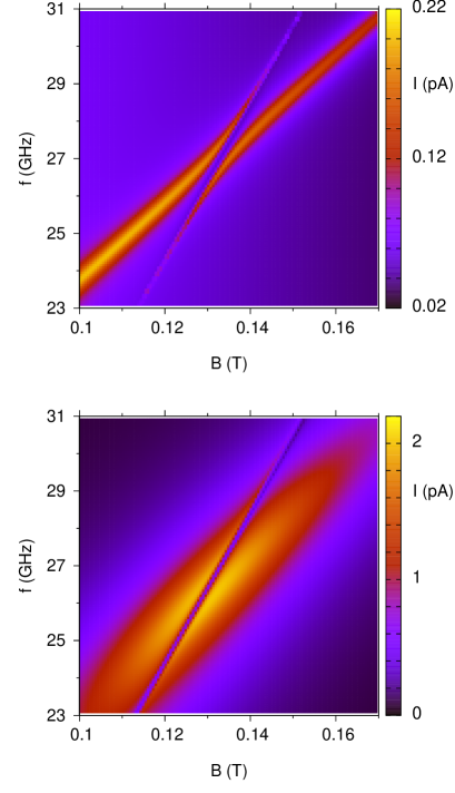
Figure 2: Current as a function of ac frequency and magnetic field. For the upper frame the ac amplitude is $A=5$ $\mu$eV, and for the lower frame $A=100$ $\mu$eV.

III ac-induced transport characteristics

In this section the ac-induced current is computed for different ac field frequencies and amplitudes, and the focus is on the two transitions which are depicted schematically in the upper frame of Fig. 1. The dot-lead tunnelling rate is $\Gamma=170$ MHz, and the energy detuning is $\varepsilon=50$ $\mu$eV unless otherwise specified.

III.1 Current versus ac frequency

Figure 2 shows the current as a function of the ac field frequency and magnetic field for two different ac amplitudes $A$. The frequency and magnetic field ranges are sensitive to the energy detuning ($\varepsilon=50$ $\mu$eV). Larger values of detuning require higher magnetic fields and ac frequencies, but ac frequencies on the order of 50 GHz are within experimental reach. fujisawa1 ; fujisawa2 When $A=5$ $\mu$eV two curves of high-current are formed. These curves can be attributed to the two singlet-triplet resonant transitions depicted schematically in Fig. 1. When the condition $hf\approx E_{5}-E_{1}$ or $hf\approx E_{5}-E_{2}$ is satisfied an ac-induced current peak is formed. The peak width is sensitive to the character of the involved states, and the peak is broad when the singlet character dominates over the triplet. For this reason the visibility of the two curves of high current is enhanced near the anticrossing point, i.e., $f\approx 27$ GHz and $B\approx 0.134$ T. Away from the anticrossing point the SOI induced singlet-triplet coupling weakens and the two curves acquire very different widths. The reason is that for the transition between $|\psi_{1}\rangle$ and $|\psi_{5}\rangle$ both involved states have triplet character, whereas for the transition between $|\psi_{2}\rangle$ and $|\psi_{5}\rangle$ the state $|\psi_{2}\rangle$ has singlet character. In essence, for $A=5$ $\mu$eV the two curves of high current map-out the singlet-triplet energy levels, and the SOI gap which is about 0.7 GHz, can be directly extracted from the current plot. This procedure has been demonstrated experimentally in different types of double quantum dots. perge12 ; ono17

In contrast, when the ac amplitude is $A=100$ $\mu$eV, as shown in Fig. 2, the two curves of high current can no longer be clearly distinguished. Moreover, when the condition $(g_{1}+g_{2})\mu_{\mathrm{B}}B=hf$ is satisfied an “antiresonance” is formed, i.e., the ac-induced current is approximately equal to the background current ($A=0$). The antiresonance is more pronounced near the anticrossing point ($f\approx 27$ GHz, $B\approx 0.134$ T). At a fixed field $B$, the frequency $f$ at which the antiresonance is formed, is not explicitly related to the ac amplitude. However, we show below that when the ac amplitude increases the ac induced current peaks start to overlap favoring the observation of the antiresonance.

It has been demonstrated ono17 that the ac-induced current peaks vanish very near the anticrossing point, when the ac-induced transitions involve the two eigenstates ($|\psi_{1}\rangle$ and $|\psi_{2}\rangle$) which form the anticrossing. The results in Fig. 2 demonstrate that the effect of the ac field can be different when the transitions include a third eigenstate not explicitly involved in the anticrossing. This is due to the large population difference between the eigenstates. In particular, the eigenstate $|\psi_{5}\rangle$ has triplet-like character, therefore it is highly populated, whereas very near the anticrossing $|\psi_{1}\rangle$ and $|\psi_{2}\rangle$ have almost identical characters and are almost equally populated. As a result, the effective transition rate between $|\psi_{5}\rangle$ and $|\psi_{1}\rangle$ (or $|\psi_{2}\rangle$) is much higher compared to the rate between $|\psi_{1}\rangle$ and $|\psi_{2}\rangle$. The peak height is sensitive to the dot-lead tunnelling rate $\Gamma$, and increasing $\Gamma$ at fixed ac amplitude $A$ tends to suppress the peaks.

Based on the results in Fig. 2 we can conclude that the singlet-triplet energy levels which anticross cannot be probed at arbitrary ac amplitudes. This conclusion sets an important constraint on the ac amplitude. In some transport experiments, perge12 ; ono17 the detection of a singlet-triplet anticrossing gap with an ac field is a reliable signature of the presence and strength of the SOI. However, the results in Fig. 2 suggest that the SOI when combined with an ac electric field can produce current characteristics which do not explicitly reveal the anticrossing gap. Thus, the detection of the SOI gap requires the appropriate choice of the ac amplitude.

Figure 3: Resonant current (peak height) as a function of magnetic field for $A=5$ $\mu$eV, and different spin-orbit tunnel couplings.

In Fig. 3, we tune the magnetic field in the range 0.1 T $\leq B\leq 0.2$ T and plot, for each $B$ the resonant current, i.e., the peak height. Here, we take note1 $A=5$ $\mu$eV and different SOI tunnel couplings $t_{\mathrm{so}}$. The peak corresponds to the magnetic field dependent ac frequency, namely, $f=(E_{5}-E_{i})/h$, where $E_{i}$ is the energy level of the state with singlet character, and therefore $i=1$ or 2 (see also Fig. 1). The peak height increases with $t_{\mathrm{so}}$ since the singlet-triplet mixing increases leading to an enhanced transition rate. The $B$ field at which the peak height is maximum depends on $t_{\mathrm{so}}$, and can be different from the anticrossing point ($B\approx 0.134$ T). This shows the overall importance of the background populations (defined for $A=0$) of the eigenstates, which are sensitive to $t_{\mathrm{so}}$ and also to the $B$ field. giavaras13 In this context, the $g$-factor difference between the two dots affects the populations by coupling $|T_{0}\rangle$ to singlet states, but the results in Fig. 2 demonstrate that the SOI anticrossing point can be probed even when the maximum current occurs away from the anticrossing point.

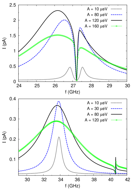
Figure 4: Current as a function of ac frequency for different ac amplitudes. For the upper frame the magnetic field is $B=0.134$ T, and for the lower frame $B=0.2$ T.

To examine in more detail the pattern of the current, we plot in Fig. 4 the current as a function of the ac frequency $f$ for various ac amplitudes $A$. In this case we choose two fixed values for the magnetic field; $B=0.134$ T which corresponds to the anticrossing point, and $B=0.2$ T which is far from the anticrossing point. When $A$ is small two peaks can be identified that are centered at the resonant frequencies $f_{1}$ and $f_{2}$ where $hf_{i}\approx E_{5}-E_{i}$, $i=1$, 2. Consequently, the corresponding singlet-triplet splitting is approximately given by $h(f_{2}-f_{1})$. Increasing $A$ results in broader peaks which gradually start to overlap; this behaviour is more evident at $B=0.134$ T. Provided $A$ is small enough such that the peaks have negligible overlap, an approximate expression for the transition rates in the coherent regime can be derived using a similar methodology to that developed in Ref. giavaras19, . For large $A$ Landau-Zener dynamics is relevant and one case for a four-level quantum dot system has been studied recently. shev

As seen in Fig. 4 the peak height is in general different for the two values of magnetic field. This is due to the fact that the transition rates as well as the background populations ($A=0$) of the eigenstates involved in the transitions are in general magnetic field dependent, even for $g_{2}\approx g_{1}$. The peak height also changes significantly with $A$. According to Fig. 4 the peak height increases with $A$ up to a maximum value and then starts to decrease. For $B=0.2$ T the maximum occurs at $A\approx 30$ $\mu$eV, and for $B=0.134$ T the maximum occurs at $A\approx 120$ $\mu$eV. The dependence of the current on the ac amplitude is examined below.

Figure 5: The figure shows the distance $\Delta_{\mathrm{p}}$ between the two ac-induced current peaks which are centered at the left and right of the antiresonance, for different ac amplitudes $A$. The dotted line denotes the value of the SOI anticrossing gap derived from the two-electron eigenenergies. The magnetic field corresponds to the anticrossing point $B=0.134$ T, and the spin-orbit tunnel coupling $t_{\mathrm{so}}$ is indicated in each frame.

A current antiresonance has been theoretically predicted to arise in a Coulomb blockaded DD in the presence of two microwave fields, brandes and in a spin blockaded DD with a Zeeman asymmetry which is driven by an oscillating magnetic field. giavaras10 A current antiresonance can also be formed without a microwave irradiation. sun The important conclusion of this section, i.e., the SOI anticrossing point cannot be probed at arbitrary ac amplitudes, is independent of the formation of the antiresonance, and the $g$-factor difference.

According to Fig. 4 (upper frame), when the magnetic field corresponds to the anticrossing point $B=0.134$ T, the ac-induced current peaks versus the ac frequency may be used to estimate the values of the SOI gap, under the condition that the ac amplitude $A$ is small. To quantify this condition we measure the distance $\Delta_{\mathrm{p}}$ between the two current peaks centered at the left and right of the antiresonance, and compare $\Delta_{\mathrm{p}}$ with the exact value of the SOI gap derived from the exact two-electron eigenenergies of the Hamiltonian Eq. (1) (for $A=0$). Figure 5 shows the distance $\Delta_{\mathrm{p}}$ between the peaks for different ac amplitudes $A$, and three values for the tunnel coupling $t_{\mathrm{so}}$. The exact value of the SOI gap is also indicated. In all cases, when $A\lesssim 35$ $\mu$eV, the value of the distance $\Delta_{\mathrm{p}}$ predicts the value of the exact SOI gap with a small error. The relative error decreases with $t_{\mathrm{so}}$ because the corresponding SOI gap increases. As an example, for $A\approx 30$ $\mu$eV, the relative error is about 11$\%$ for $t_{\mathrm{so}}=0.5$ $\mu$eV, whereas the relative error is about 0.6$\%$ for $t_{\mathrm{so}}=3.0$ $\mu$eV. An important aspect is that the peak width depends not only on the ac amplitude but also on the strength of the SOI which in our model is determined by the tunnel coupling $t_{\mathrm{so}}$, and the energy detuning $\varepsilon$. The reason is that, for the parameter range of this work, the ac-induced transition rates are enhanced with $t_{\mathrm{so}}$, and the electrically driven transitions we study here vanish when $t_{\mathrm{so}}=0$. The results in Fig. 5 also demonstrate that the error tends to increase with $A$, since the two peaks start to overlap and shift (Fig. 4), and as a consequence the value of $\Delta_{\mathrm{p}}$ deviates from the exact SOI gap.

Even though a smaller ac amplitude can lead to a more accurate estimation of the SOI gap, the dot-lead tunnelling rate $\Gamma$ sets another constraint on the ac amplitude $A$. A small $A$ can give rise to coherent effects only when $\Gamma$ is small, eventually inducing a small current which might be difficult to measure. Measuring the ac-induced current peaks for only one value of the ac amplitude may not be conclusive because the degree of overlap of the current peaks cannot be inferred. Therefore, a more efficient strategy to probe the SOI gap would be to tune the ac amplitude and monitor the behaviour of the current peaks.

III.2 Approximate Hamiltonian

Some insight into the current characteristics can be obtained within an approximate time independent Hamiltonian. It has been shown that a single spin driven by an alternating magnetic field displays resonances (single or multiphoton) when the two Floquet energies anticross. shirley This property is general enough and has been employed to predict the existence of resonances for two coupled spins whose energy levels are time dependent. satanin ; shevchenko In this context, the eigenenergies of the approximate time independent Hamiltonian should also exhibit anticrossing points when a resonance occurs. This remark is relevant when the starting point is the exact Floquet Hamiltonian, as well as when deriving an approximate Hamiltonian without directly employing the Floquet formalism.

To derive an approximate Hamiltonian we start with the time dependent DD Hamiltonian Eq. (1), and apply a unitary transformation $U(t)$. The nonzero diagonal elements are $U_{nm}(t)=\delta_{nm}\exp[i\phi_{n}(t)]$, and the phases are $\phi_{3}=-\sin(2\pi ft)A/hf$, $\phi_{4}=-2\pi ft$, otherwise $\phi_{n}=0$. This transformation eliminates the time dependence from the energy detuning and transfers it to the tunnel couplings. It also shifts downwards by $-hf$ the bare energy level $\Delta^{+}$ of $|T_{-}\rangle$, because near the anticrossing point we are interested in the transitions satisfying $\Delta^{+}-hf\approx-\Delta^{+}$, where $-\Delta^{+}$ is the bare energy level of $|T_{+}\rangle$. The transformed Hamiltonian is

$$W=\left(\begin{array}[]{ccccc}0&0&\sqrt{2}T_{\mathrm{c}}&0&\Delta^{-}\\ 0&-\Delta^{+}&a_{\mathrm{so}}&0&0\\ \sqrt{2}T^{*}_{\mathrm{c}}&a^{*}_{\mathrm{so}}&-\varepsilon&b_{\mathrm{so}}&0\\ 0&0&b^{*}_{\mathrm{so}}&\Delta^{+}-hf&0\\ \Delta^{-}&0&0&0&0\\ \end{array}\right),$$ (10)

and the tunnel couplings are

$$\begin{split}T_{\mathrm{c}}=-t_{\mathrm{c}}\sum^{\infty}_{m=-\infty}(-1)^{m}J_{m}e^{im2\pi ft},\\ a_{\mathrm{so}}=-t_{\mathrm{so}}\sum^{\infty}_{m=-\infty}(-1)^{m}J_{m}e^{im2\pi ft},\\ b_{\mathrm{so}}=-t_{\mathrm{so}}\sum^{\infty}_{m=-\infty}J_{m}e^{i(m-1)2\pi ft},\end{split}$$ (11)

where $J_{m}$ is a Bessel function of the first kind with the argument $A/hf$ $[J_{m}=J_{m}(A/hf)]$. This Hamiltonian is exact, and we proceed by assuming that the time independent terms of this Hamiltonian can well describe the relevant dynamics. Thus, in the above tunnel couplings we ignore all the time dependent terms:

$$T_{\mathrm{c}}=-t_{\mathrm{c}}J_{0},\quad a_{\mathrm{so}}=-t_{\mathrm{so}}J_{0},\quad b_{\mathrm{so}}=-t_{\mathrm{so}}J_{1},$$ (12)

and in the transformed (moving) frame we arrive at an approximate time independent Hamiltonian $W_{0}$ which has some interesting properties.

For example, the energy spectrum of $W_{0}$ can be used to predict the current resonances by examining the formation of the anticrossing points. Especially in the regime $A\ll hf$, the spectrum of $W_{0}$ approximates very well the exact Floquet spectrum. Most importantly, the diagonalization of $W_{0}$ reveals the existence of the eigenstate note2

$$c_{+}|T_{+}\rangle+c_{-}|T_{-}\rangle,$$ (13)

when $\Delta^{+}=hf/2$ or, equivalently, $(g_{1}+g_{2})\mu_{\mathrm{B}}B=hf$, with the coefficients $c_{+}/c_{-}=-J_{1}/J_{0}$. This eigenstate contains no $|S_{02}\rangle$ component, which is responsible for the current; therefore, it acts as a “dark” eigenstate. Namely, it does not allow the ac field to enhance the current, and consequently, the ac-induced current ($A\neq 0$) is approximately equal to the background current ($A=0$). This dark eigenstate which has a Bell-like structure, is the origin of the current antiresonance described above (e.g. Fig. 2). As also emphasized, the antiresonance exists independent of the magnitude of the ac amplitude as well as for a vanishingly small $g$-factor difference, in agreement with the existence of the dark eigenstate predicted by $W_{0}$.

The predictions of the approximate Hamiltonian $W_{0}$ are accurate enough in the regime where $\Delta^{+}$ is different from $\varepsilon$, but when $\Delta^{+}\approx\varepsilon$ another treatment can be sought for improved accuracy. note3 This observation can be understood by inspecting the exact Floquet Hamiltonian as derived now from $W(t)$ instead of $H_{\mathrm{DD}}(t)$. In particular, the coupling terms between the diagonal elements $W_{ii}\pm nhf$ of the Floquet Hamiltonian suggest that a general Floquet mode should include at least the basis states $\exp(in2\pi ft)|S_{11}\rangle$, $n=0$, 1. The coupling terms which involve Bessel functions $J_{m}$ with $|m|>1$ can typically be ignored within an approximate Floquet Hamiltonian. Some additional properties of $W_{0}$ are examined in Sec. III.C, where the dependence of the ac-induced current peaks on the ac amplitude is investigated.

III.3 Current versus ac amplitude

Figure 6: Current as a function of ac amplitude $A$ at fixed magnetic field $B=0.134$ T. For the solid line the ac frequency is $f=26.53$ GHz and the SOI tunnel coupling is $t_{\mathrm{so}}=3$ $\mu$eV. For the dotted line $f=26.85$ GHz and $t_{\mathrm{so}}=1.5$ $\mu$eV. In both cases the frequency satisfies $f=(E_{5}-E_{2})/h$ as depicted in Fig. 1. The inset shows $J^{2}_{m}(r)$, $m=0$, 1 for $0<r<10$.

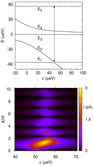
Figure 7: The upper frame shows the two-electron eigenenergies as a function of energy detuning for the magnetic field $B=0.134$ T. The vertical arrow at the anticrossing point $\varepsilon\approx 50$ $\mu$eV specifies the ac frequency $f$ used in the lower frame, specifically, $f=(E_{5}-E_{2})/h=26.85$ GHz. The lower frame shows the current as a function of energy detuning and ac amplitude at fixed frequency $f=26.85$ GHz and magnetic field $B=0.134$ T.

According to Fig. 4 the height of the current peaks induced by the ac field depends sensitively on the ac amplitude $A$, and exhibits a non-monotonous behaviour. Furthermore, the approximate Hamiltonian $W_{0}$ reveals the possibility of tuning the DD system to the so-called “coherent destruction of tunnelling” regime, flqmas2 ; destruct1 ; destruct2 ; destruct3 ; destruct4 where the inter-dot tunnel coupling vanishes for specific values of the ratio $A/hf$. In our ac driven DD there are three effective tunnel coupling terms given in Eq. (12), which are sensitive to the ratio $A/hf$. When $J_{0}(A/hf)=0$ the spin-conserved tunnel coupling vanishes, $T_{\mathrm{c}}=0$, and therefore $|S_{11}\rangle$ and $|T_{0}\rangle$ are blocked states ($|\uparrow,\downarrow\rangle$, $|\downarrow,\uparrow\rangle$) because they cannot coherently tunnel to the $|S_{02}\rangle$ singlet. Simultaneously, when $J_{0}(A/hf)=0$ the SOI spin-flipped tunnel coupling between the $|T_{+}\rangle$ and $|S_{02}\rangle$ states vanishes because $a_{\mathrm{so}}=0$, and thus $|T_{+}\rangle$ is also a blocked state. In this regime, the ac-induced current should be suppressed because only the $|T_{-}\rangle$ state is tunnel-coupled to the $|S_{02}\rangle$ state. Similarly, the current should also be somewhat suppressed when $J_{1}(A/hf)=0$, because the SOI tunnel coupling between the $|T_{-}\rangle$ and $|S_{02}\rangle$ states vanishes ($b_{\mathrm{so}}=0$) and now $|T_{-}\rangle$ acts as a blocked state.

To study the dependence of the ac-induced current on the ac amplitude we focus on the transition between $|\psi_{5}\rangle$ and $|\psi_{2}\rangle$, so that the ac frequency is $f=(E_{5}-E_{2})/h$, and use the equation of motion [Eq. (7)] to determine the current characteristics in the steady state. In Fig. 6 we plot the current as a function of the ac amplitude for $t_{\mathrm{so}}=1.5$ $\mu$eV and $t_{\mathrm{so}}=3$ $\mu$eV. For these two cases the frequency $f$ is different since the SOI gap is different. For convenience, we also plot $J^{2}_{m}$, $m=0$, 1. Some of the current characteristics can be understood using the above arguments regarding the formation of blocked states. For example, the current displays a local minimum (it is suppressed) when either $J_{0}=0$ or $J_{1}=0$. Moreover, in the asymptotic regime, defined for $A>2.5hf$, the current displays an oscillatory behaviour and the overall current decreases following the overall reduction in the interdot tunnel coupling terms [Eq. (12)] between the spin blocked states and the $|S_{02}\rangle$ singlet state. In Fig. 6 the field corresponds to the anticrossing $B\approx 0.134$ T, but the SOI forms another anticrossing at $B\approx 0.014$ T (Fig. 1). At this field the ac-induced current due to the transitions between $|\psi_{2}\rangle$ and $|\psi_{4}\rangle$ (or $|\psi_{5}\rangle$) has different form from that in Fig. 6, but these transitions are not considered in the present work.

As seen in Fig. 6 for $A\lesssim 2.5hf$, two regimes can be identified. Specifically, as the amplitude $A$ increases, the current first increases and then it starts to decrease. The increase of the current is expected because the ac field induces transitions (Fig. 1) between states with different populations; a state with mostly triplet character and high population ($|\psi_{5}\rangle$), and a state with large $|S_{02}\rangle$ component and lower population ($|\psi_{2}\rangle$). The approximate Hamiltonian $W_{0}$ suggests that the increase of the current is related to the increase of the tunnel coupling term $b_{\mathrm{so}}$. This term gradually lifts the (partial) spin blockade due to the blocked $|T_{-}\rangle$ state, by allowing transitions from $|T_{-}\rangle$ to $|S_{02}\rangle$. However, the tunnel couplings $a_{\mathrm{so}}$ and $T_{\mathrm{c}}$ decrease with $A$; therefore, the current should reach a maximum value and then should start to decrease. The crossover point is sensitive to the exact frequency (magnetic field) and the dot-lead rate $\Gamma$. The largest ac amplitude $A$ considered in this work is on the order of 1.5 meV (when $A\approx 10hf$), and such relatively large amplitude can usually be generated in quantum dot systems by applying electrical pulses. perge12 ; ono17 ; bertrand ; pulses1 Electrical noise in quantum dots is device dependent and may influence the current characteristics, but coherent effects due to the ac field have been demonstrated in various devices when the noise level is low, enabling transport spectroscopy of spin states and estimation of the spin-orbit gap. perge12 ; ono17

In double quantum dots the energy detuning can usually be controlled by gate voltages, hanson07 and thus it is interesting to explore the detuning dependence of the ac-induced current near the SOI singlet-triplet anticrossing point. For convenience in the upper frame of Fig. 7 we plot the two-electron eigenenergies as a function of the energy detuning ($A=0$) for the magnetic field $B=0.134$ T. The anticrossing point which is formed at $\varepsilon=0$ is due to the $|S_{11}\rangle$, $|S_{02}\rangle$ coupling and it exists even for zero SOI. Here, we focus on the region near the SOI singlet-triplet anticrossing point, formed at $\varepsilon\approx 50$ $\mu$eV, and plot in the lower frame of Fig. 7 the current as a function of the energy detuning and ac amplitude. For all the calculations, the Floquet-Markov equation of motion Eq. (7) is used again. The field is $B=0.134$ T and the ac frequency is $f=26.85$ GHz with $f=(E_{5}-E_{2})/h$ at $\varepsilon\approx 50$ $\mu$eV. Therefore, we refer to this particular detuning as the “resonant” detuning where the current is expected to be high, whereas for this particular case under study $f\neq(E_{5}-E_{1})/h$ at any $\varepsilon$.

In Fig. 7, a high-current region can be identified in the detuning range $47$ $\mu$eV $\lesssim\varepsilon\lesssim$ 62 $\mu$eV, especially for $A/hf\lesssim 2.5$. This range of the detuning includes the resonant detuning value as well as the two detuning values satisfying the resonant conditions suggested by the approximate Hamiltonian $W_{0}$, i.e., $\varepsilon\approx\Delta^{+}$ and $\varepsilon\approx hf-\Delta^{+}$ which give $\varepsilon\approx 54.7$ $\mu$eV and $\varepsilon\approx 56.2$ $\mu$eV respectively. These two values are greater than the resonant detuning, and as a result the extent of the high-current region along the detuning axis is larger for $\varepsilon>50$ $\mu$eV. But, for $\varepsilon<50$ $\mu$eV the high-current region decays faster as the system is gradually tuned off resonance. When the ac amplitude increases for $A/hf>2.5$, the current displays minima at the values of $A/hf$ which generate ac-induced blocked states, $J_{0}=0$ or $J_{1}=0$, and the current pattern is similar to that presented in Fig. 6. The minima have a characteristic wide shape off resonance which becomes narrower near a resonance where the current increases. The details of the pattern of the current versus $A$ and $\varepsilon$, depend on the choice of the exact ac frequency $f$. In Fig. 7, the frequency is $f=(E_{5}-E_{2})/h$ but a very similar pattern occurs for $f=(E_{5}-E_{1})/h$, and in general for choices of frequencies away from the anticrossing point. The high-current regions can be easily identified by considering the corresponding resonant conditions which involve the parameters $\varepsilon$, $f$ and $\Delta^{+}$. In contrast, the current is in general lower off resonance and when blocked states are formed.

IV Conclusion

In this work we considered a double quantum dot in the spin blockade regime and in the presence of an ac electric field which periodically changes the energy detuning. We focused on specific energy configurations (Fig. 1) which involve two SOI-coupled singlet-triplet states forming an anticrossing point, and a third state with mostly triplet character. We studied the electronic transport characteristics at the anticrossing point and found strong ac-induced current peaks, in contrast to the vanishingly small peaks observed for a pair of singlet-triplet states. ono17 We showed that for small ac field amplitudes the current peaks map-out the two-electron energy levels and the SOI-induced anticrossing point. In this case, the gap of the anticrossing can be estimated, giving direct information about the strength of the SOI. As the ac amplitude increases, the resonant pattern changes drastically and a current antiresonance is formed. Eventually, the SOI anticrossing point can no longer be probed. We examined the ac-induced current versus the ac amplitude and showed that current suppression can take place when the ac field gives rise to blocked states for specific values of the ac amplitude and ac frequency. As a result, the pattern of the current consists of low- and high-current regions, which can be controlled by the ac field.

The weak driving regime in which the resonant current peaks map-out the SOI anticrossing point has been demonstrated in different double quantum dot systems. However, the stronger driving regime in which the resonant current peaks strongly overlap and/or coherent interdot tunnelling is suppressed seems to remain unexplored. In our work, we demonstrated a realistic range of parameters for which the crossover from the weak to the strong driving regime can be identified, and pointed out possible experimental implications.

Appendix A Double dot in the spin blockade

In this appendix we derive the double quantum dot Hamiltonian used in the main article. Specifically, we employ the two-site Hubbard Hamiltonian

$$\begin{split}&h_{\mathrm{DD}}=\sum_{i=1}^{2}\epsilon_{i}(n_{i\uparrow}+n_{i\downarrow})+\sum_{i=1}^{2}U_{i}n_{i\uparrow}n_{i\downarrow}\\ &+\frac{1}{2}\sum_{i=1}^{2}g_{i}\mu_{\mathrm{B}}B(n_{i\downarrow}-n_{i\uparrow})+Vn_{1}n_{2}+h_{\mathrm{T}},\end{split}$$ (14)

which allows for up to two electrons on each dot $i$ with $i=1$, 2. We define the number operator $n_{i}=n_{i\uparrow}+n_{i\downarrow}$ with $n_{i\sigma}=c_{i\sigma}^{\dagger}c_{i\sigma}$ for dot $i$ and spin $\sigma=\uparrow,\downarrow$. The fermionic operator $c_{i\sigma}^{\dagger}$ ($c_{i\sigma}$) creates (annihilates) an electron on dot $i$ with on-site orbital energy $\epsilon_{i}$. The Zeeman splitting on dot $i$ due to the applied magnetic field $B$ is equal to $g_{i}\mu_{\mathrm{B}}B$, where $g_{i}$ is the $g$-factor of dot $i$, and $\mu_{\mathrm{B}}$ is the Bohr magneton. When two electrons occupy the same dot $i$ the intradot Coulomb energy is $U_{i}$, and when two electrons occupy different dots the interdot Coulomb energy is $V$.

The two dots are tunnel-coupled and tunnelling between the two dots is modelled by the Hamiltonian $h_{\mathrm{T}}=h_{\mathrm{c}}+h_{\mathrm{so}}$, with

$$h_{\mathrm{c}}=-t_{\mathrm{c}}\sum_{\sigma}(c_{1\sigma}^{\dagger}c_{2\sigma}+\text{H.c.}),$$ (15)

and

$$h_{\mathrm{so}}=t_{\mathrm{so}}(c_{1\uparrow}^{\dagger}c_{2\downarrow}-c_{1\downarrow}^{\dagger}c_{2\uparrow}+\text{H.c.}).$$ (16)

The Hamiltonian $h_{\mathrm{c}}$ describes electron tunnelling between the two dots with coupling $t_{\mathrm{c}}$, which measures the degree of overlap between the states localized in different quantum dots. The Hamiltonian $h_{\mathrm{so}}$ accounts for a Rashba-like spin-orbit interaction, romeo ; pan ; mireles and induces interdot tunnelling via a spin-flip with coupling $t_{\mathrm{so}}$. This coupling is inversely proportional to the spin-orbit length which is sensitive to the details of the double dot geometry as well as the direction of the applied magnetic field relative to the spin-orbit axis. perge12 ; nowak ; takahashi ; stano Because this direction is device dependent, in our work we assume different couplings $t_{\mathrm{so}}$ in the regime $t_{\mathrm{so}}<t_{\mathrm{c}}$ which is in agreement with other studies. perge12 ; ono17 ; wang ; chorley11 The microscopic details of the spin-orbit interaction are not important in our work, since the key requirement for the formation of the ac-induced peaks studied in the main article is the nonzero coupling $t_{\mathrm{so}}$. As shown below the Hamiltonian $h_{\mathrm{c}}$ can only hybridize singlet states, in contrast, the Hamiltonian $h_{\mathrm{so}}$ leads to hybridized singlet-triplet states. Therefore, both $h_{\mathrm{c}}$ and $h_{\mathrm{so}}$ form anticrossing points in the energy spectrum and the degree of state hybridization is maximum in the vicinity of these points.

So far, the double dot Hamiltonian Eq. (14) is general enough and not specific to the spin blockade regime. We now focus on the spin blockade regime and without loss of generality, we assume for simplicity that $U_{1}=U_{2}=U$, $V=0$, and choose for the orbital energies

$$\epsilon_{1}=+\frac{U}{2}+\frac{\varepsilon}{2},\qquad\epsilon_{2}=-\frac{U}{2}-\frac{\varepsilon}{2},$$ (17)

with the parameters satisfying $U\gg t_{\mathrm{c}}$, $|\varepsilon|$. Specifically, the charging energy $U$ can be as large as 10-20 meV, whereas $t_{\mathrm{c}}$ is typically less than 1 meV. The energy detuning $\varepsilon$ is usually tunable with electrostatic gates, and quantifies the energy difference,

$$\varepsilon=E(1,1)-E(0,2).$$ (18)

The notation $E(n,m)$ denotes the energy of the bare charge state with $n$ ($m$) electrons on dot 1 (dot 2). The single electron states of the Hilbert space are $c^{\dagger}_{i\sigma}|0\rangle$ with $i=1$, 2, spin $\sigma=\uparrow,\downarrow$ and $|0\rangle$ is the vacuum state. Because of the small ratio $t_{\mathrm{c}}/(\epsilon_{1}-\epsilon_{2})$, the hybridization between dot 1 states and dot 2 states is typically very small.

The two-electron states of the Hilbert space are:

$$\begin{split}&|S_{20}\rangle=c^{\dagger}_{1\uparrow}c^{\dagger}_{1\downarrow}|0\rangle,\quad|T_{+}\rangle=c^{\dagger}_{1\uparrow}c^{\dagger}_{2\uparrow}|0\rangle,\\ &|\uparrow,\downarrow\rangle=c^{\dagger}_{1\uparrow}c^{\dagger}_{2\downarrow}|0\rangle,\quad|\downarrow,\uparrow\rangle=c^{\dagger}_{1\downarrow}c^{\dagger}_{2\uparrow}|0\rangle,\\ &|T_{-}\rangle=c^{\dagger}_{1\downarrow}c^{\dagger}_{2\downarrow}|0\rangle,\quad|S_{02}\rangle=c^{\dagger}_{2\uparrow}c^{\dagger}_{2\downarrow}|0\rangle.\end{split}$$ (19)

Alternatively, we can define states with definite spin number, i.e., singlet states: $|S_{20}\rangle$, $|S_{11}\rangle=(|\uparrow,\downarrow\rangle-|\downarrow,\uparrow\rangle)/\sqrt{2}$, $|S_{02}\rangle$ and triplet states: $|T_{-}\rangle$, $|T_{0}\rangle=(|\uparrow,\downarrow\rangle+|\downarrow,\uparrow\rangle)/\sqrt{2}$, $|T_{+}\rangle$. The energy of the state $|S_{20}\rangle$, e.g., when two electrons occupy dot 1, is $E(2,0)=2\epsilon_{1}+U=2U+\varepsilon$, whereas the energy of all states with one electron on each dot is $E(1,1)=\epsilon_{1}+\epsilon_{2}=0$, and the energy of the $|S_{02}\rangle$ state is $E(0,2)=2\epsilon_{2}+U=-\varepsilon$. Because of the large energy scale difference (on the order of $2U$) the state $|S_{20}\rangle$ has a minor effect on the spin blockade physics and can be ignored. As a result, there are five relevant two-electron states in the spin blockade regime:

$$|S_{11}\rangle,\quad|T_{+}\rangle,\quad|S_{02}\rangle,\quad|T_{-}\rangle,\quad|T_{0}\rangle.$$ (20)

At low temperatures (0.1 K) three- and four-electron states are not involved in the transport cycle and can be ignored. Furthermore, when the Fermi energy of the right lead $E_{\mathrm{F}}$ satisfies $\epsilon_{2}<E_{\mathrm{F}}<\epsilon_{2}+U$, a single electron occupies dot 2 during the transport cycle while a second electron is allowed to tunnel from dot 2 to the right lead.

To account for the effect of the ac electric field we assume that the orbital energies of the two dots are modulated in a “symmetric way”, thus,

$$\begin{split}&\epsilon_{1}=+\frac{U}{2}+\frac{\varepsilon}{2}-\frac{A}{2}\cos(2\pi ft),\\ &\epsilon_{2}=-\frac{U}{2}-\frac{\varepsilon}{2}+\frac{A}{2}\cos(2\pi ft).\end{split}$$ (21)

The amplitude of the ac field is $A$ and the frequency is $f$. The assumption of symmetric modulation is not unique; we can equivalently assume, for instance, that $\epsilon_{1}$ is unaffected by the ac field and $\epsilon_{2}=-\frac{U}{2}-\frac{\varepsilon}{2}+A\cos(2\pi ft)$. In this case the conclusions in the main article remain unchanged. The particular choice in Eq. (21) allows us to define the time dependent energy detuning

$$\delta=-\varepsilon+A\cos(2\pi ft),$$ (22)

and write the orbital energies as

$$\epsilon_{1}=+\frac{U}{2}-\frac{\delta}{2},\quad\epsilon_{2}=-\frac{U}{2}+\frac{\delta}{2}.$$ (23)

Then, in the two-electron basis $|S_{11}\rangle$, $|T_{+}\rangle$, $|S_{02}\rangle$, $|T_{-}\rangle$, $|T_{0}\rangle$, the Hamiltonian $h_{\mathrm{DD}}$ has the form given in Eq. (1) in the main article. This approximate Hamiltonian is valid in the spin blockade regime and has also been employed in other works. perge12 ; giavaras19 ; pei ; giavarasE From this Hamiltonian we see that the only time dependent term corresponds to the energy of the $|S_{02}\rangle$ singlet state (diagonal term) and is equal to the detuning $\delta$. Even though, the Coulomb energy $U$ is the largest energy scale, it does not explicitly appear in the Hamiltonian because the $|S_{20}\rangle$ state is ignored. The Hamiltonian Eq. (1) in the main article also shows that when $A=0$ the $|S_{02}\rangle$, $|S_{11}\rangle$ states are hybridized due to the $t_{\mathrm{c}}$ term, and similarly the $|S_{02}\rangle$, $|T_{\pm}\rangle$ states are hybridized due to the $t_{\mathrm{so}}$ term. In particular, the ac-induced current peaks studied in the main article are formed only when $t_{\mathrm{so}}\neq 0$.

References

- (1) R. Hanson, L. P. Kouwenhoven, J. R. Petta, S. Tarucha, and L. M. K. Vandersypen, Rev. Mod. Phys. 79, 1217 (2007).
- (2) F. A. Zwanenburg, A. S. Dzurak, A. Morello, M. Y. Simmons, L. C. L. Hollenberg, G. Klimeck, S. Rogge, S. N. Coppersmith, and M. A. Eriksson, Rev. Mod. Phys. 85, 961 (2013).
- (3) S. Nadj-Perge, V. S. Pribiag, J. W. G. van den Berg, K. Zuo, S. R. Plissard, E. P. A. M. Bakkers, S. M. Frolov, and L. P. Kouwenhoven, Phys. Rev. Lett. 108, 166801 (2012).
- (4) K. Ono, G. Giavaras, T. Tanamoto, T. Ohguro, X. Hu, and F. Nori, Phys. Rev. Lett. 119, 156802 (2017).
- (5) Z.-H. Liu, O. Entin-Wohlman, A. Aharony, and J. Q. You, Phys. Rev. B 98, 241303(R) (2018).
- (6) Z.-H. Liu, R. Li, X. Hu, and J. Q. You, Sci. Rep. 8, 2302 (2018).
- (7) M. P. Nowak, B. Szafran, F. M. Peeters, B. Partoens, and W. J. Pasek, Phys. Rev. B 83, 245324 (2011).
- (8) S. Takahashi, R. S. Deacon, K. Yoshida, A. Oiwa, K. Shibata, K. Hirakawa, Y. Tokura, and S. Tarucha, Phys. Rev. Lett. 104, 246801 (2010).
- (9) Y. Kanai, R. S. Deacon, S. Takahashi, A. Oiwa, K. Yoshida, K. Shibata, K. Hirakawa, Y. Tokura, and S. Tarucha, Nature Nanotechnology 6, 511 (2011).
- (10) P. Stano and J. Fabian, Phys. Rev. Lett. 96, 186602 (2006).
- (11) C. Fasth, A. Fuhrer, L. Samuelson, V. N. Golovach, and D. Loss, Phys. Rev. Lett. 98, 266801 (2007).
- (12) G. Giavaras and Y. Tokura, Phys. Rev. B 99, 075412 (2019).
- (13) K. Ono, D. G. Austing, Y. Tokura, and S. Tarucha, Science 297, 1313 (2002).
- (14) J.-Y. Wang, S. Huang, Z. Lei, D. Pan, J. Zhao, and H. Q. Xu, Appl. Phys. Lett. 109, 053106 (2016).
- (15) S. J. Chorley, G. Giavaras, J. Wabnig, G. A. C. Jones, C. G. Smith, G. A. D. Briggs, and M. R. Buitelaar, Phys. Rev. Lett. 106, 206801 (2011).
- (16) B. Bertrand, H. Flentje, S. Takada, M. Yamamoto, S. Tarucha, A. Ludwig, A. D. Wieck, C. B uerle, and T. Meunier, Phys. Rev. Lett. 115, 096801 (2015).
- (17) K. Ono, S. N. Shevchenko, T. Mori, S. Moriyama, and F. Nori, Phys. Rev. Lett. 122, 207703 (2019).
- (18) T. P. Smith III and F. F. Fang, Phys. Rev. B 35, 7729 (1987).
- (19) J. W. G. van den Berg, S. Nadj-Perge, V. S. Pribiag, S. R. Plissard, E. P. A. M. Bakkers, S. M. Frolov, and L. P. Kouwenhoven, Phys. Rev. Lett. 110, 066806 (2013).
- (20) S. Kohler, J. Lehmann, and P. Hänggi, Phys. Rep. 406, 379 (2005).
- (21) M. Grifoni and P. Hänggi, Phys. Rep. 304, 229 (1998).
- (22) J. H. Shirley, Phys. Rev. 138, B979 (1965).
- (23) F. Bloch and A. Siegert, Phys. Rev. 57, 522 (1940).
- (24) T. H. Oosterkamp, T. Fujisawa, W. G. van der Wiel, K. Ishibashi, R. V. Hijman, S. Tarucha, and L. P. Kouwenhoven, Nature 395, 873 (1998).
- (25) T. Fujisawa, T. Hayashi, and S. Sasaki, Rep. Prog. Phys. 69, 759 (2006).
- (26) A small value of amplitude makes the identification of the resonant current easier.
- (27) G. Giavaras, N. Lambert, and F. Nori, Phys. Rev. B 87, 115416 (2013).
- (28) S. N. Shevchenko, A. I. Ryzhov, and F. Nori, Phys. Rev. B 98, 195434 (2018).
- (29) T. Brandes and F. Renzoni, Phys. Rev. Lett. 85, 4148 (2000).
- (30) G. Giavaras, J. Wabnig, B. W. Lovett, J. H. Jefferson, and G. A. D. Briggs, Phys. Rev. B 82, 085410 (2010).
- (31) Z. Z. Sun, R. Q. Zhang, W. Fan, and X. R. Wang, J. Appl. Phys. 105, 043706 (2009).
- (32) A. M. Satanin, M. V. Denisenko, S. Ashhab, and F. Nori, Phys. Rev. B 85, 184524 (2012).
- (33) S. N. Shevchenko, S. Ashhab, and F. Nori, Phys. Rep. 492, 1 (2010).
- (34) For simplicity, we use the same notation for the basis states in the moving and laboratory frame.
- (35) Another transformation can be performed with the non-zero phases: , ; leading to in Eq. (12) whereas , are the same as in Eq. (12). An approximate calculation of the current using both and (when and near the anticrossing) can be in better agreement with the exact current than using only . This approximate calculation is not pursued in this work.
- (36) F. Grossmann, T. Dittrich, P. Jung, and P. Hänggi, Phys. Rev. Lett. 67, 516 (1991).
- (37) C. E. Creffield and G. Platero, Phys. Rev. B 65, 113304 (2002).
- (38) E. Paspalakis and A. Terzis, J. Appl. Phys. 95, 1603 (2004).
- (39) E. Paspalakis, Phys. Rev. B 67, 233306 (2003).
- (40) F. Romeo and R. Citro, Phys. Rev. B 80, 165311 (2009).
- (41) H. Pan and Y. Zhao, J. Appl. Phys. 111, 083703 (2012).
- (42) F. Mireles and G. Kirczenow, Phys. Rev. B 64, 024426 (2001).
- (43) T. Pei, A. Palyi, M. Mergenthaler, N. Ares, A. Mavalankar, J. H. Warner, G. A. D. Briggs, and E. A. Laird, Phys. Rev. Lett. 118, 177701 (2017).
- (44) G. Giavaras, Physica E 87, 129 (2017).