Uplink-aided High Mobility Downlink Channel Estimation over Massive MIMO-OTFS System

Abstract

Although it is often used in the orthogonal frequency division multiplexing (OFDM) systems, application of massive multiple-input multiple-output (MIMO) over the orthogonal time frequency space (OTFS) modulation could suffer from enormous training overhead in high mobility scenarios. In this paper, we propose one uplink-aided high mobility downlink channel estimation scheme for the massive MIMO-OTFS networks. Specifically, we firstly formulate the time domain massive MIMO-OTFS signal model along the uplink and adopt the expectation maximization based variational Bayesian (EM-VB) framework to recover the uplink channel parameters including the angle, the delay, the Doppler frequency, and the channel gain for each physical scattering path. Correspondingly, with the help of the fast Bayesian inference, one low complex approach is constructed to overcome the bottleneck of the EM-VB. Then, we fully exploit the angle, delay and Doppler reciprocity between the uplink and the downlink and reconstruct the angles, the delays, and the Doppler frequencies for the downlink massive channels at the base station. Furthermore, we examine the downlink massive MIMO channel estimation over the delay-Doppler-angle domain. The channel dispersion of the OTFS over the delay-Doppler domain is carefully analyzed and is utilized to associate one given path with one specific delay-Doppler grid if different paths of any user have distinguished delay-Doppler signatures. Moreover, when all the paths of any user could be perfectly separated over the angle domain, we design the effective path scheduling algorithm to map different users’ data into the orthogonal delay-Doppler-angle domain resource and achieve the parallel and low complex downlink 3D channel estimation. For the general case, we adopt the least square estimator with reduced dimension to capture the downlink delay-Doppler-angle channels. Various numerical examples are presented to confirm the validity and robustness of the proposed scheme.

I Introduction

Massive multiple-input multiple-output (MIMO) has become one of the most important enabling technologies for the 5-th generation (5G) and beyond wireless networks, due to its tremendously improved spectral and energy efficiencies [1, 2, 3, 4, 5, 6]. To fully exploit the advantages of massive MIMO, a set of designed strategies have been proposed in reducing its implementation cost and complexity [7, 8, 9, 10, 11, 12, 13, 14, 15]. However, in the high mobility scene, most of these methods do not work effectively due to the rapid channel variation.

To overcome this challenge, there are many works about the time-varying massive MIMO channels. Qin et al. proposed one effective time-varying massive MIMO channel estimation scheme for the orthogonal frequency division multiplexing (OFDM) system, where the complex exponential basis expansion model (CE-BEM) was utilized for the representation of the time-varying channels [16]. In [17], Zhao et al. designed a channel tracking method for massive MIMO systems under both time-varying and spatial-varying circumstances, where the effective dimension of the uplink (UL)/ the downlink (DL) channel was reduced by the spatial-temporal basis expansion model. In [18], Guo et al. applied angle domain Doppler compensation for high-mobility wideband massive MIMO UL communications, where the Doppler spread of the equivalent UL channel after angle domain Doppler compensation was theoretically analyzed. In [19], Ma et al. developed an expectation maximization (EM) based sparse Bayesian learning (SBL) framework to learn the spatial and temporal parameters for the time-varying massive MIMO channel model and applied a Kalman filter (KF) with reduced dimension for the channel tracking. Furthermore, in [20], Li et al. expanded the work in [19], where they considered the randomness of direction of arrivals (DOAs), focused on the imperfection of the reconstructed parameters and proposed an optimal Bayesian Kalman filtering (OBKF) method along DL. However, The aforementioned methods only consider the block-fading channel, i.e., the channel only changes from block to block. This assumption is reasonable in low velocity scenario, but may be not applicable in the high speed scenarios.

Meanwhile, the massive MIMO channels may experience the frequency-selective fading, and OFDM is usually adopted. However, for the high-mobility scenarios, OFDM may possess the significant inter-carrier interference (ICI) due to the Doppler spread of the time-variant channels, which then severely degrades the system performance. To deal with this problem, Hadani et al. designed a novel two-dimensional modulation technique called orthogonal time frequency space (OTFS) modulation [21]. Fig. 1 shows the OTFS architecture [22]. As the newly proposed modulation/demodulation technique, OTFS can be achieved through adding some function blocks to the OFDM scheme, i.e., adding a pre-processing block before a traditional OFDM modulator and a corresponding post-processing block after a traditional OFDM demodulator. With the help of the pre-processing and post-processing blocks, the time-variant channels are converted into the time-independent channels in the delay-Doppler domain. Therefore, the information bearing data can be multiplexed over the roughly constant channels in the delay-Doppler domain. At the same time, the transmitted data in OTFS systems can take full advantage of the diversity for the frequency-time channels. In this way, OTFS can improve the system performance over OFDM in the high-mobility scenarios [22]. Hence, OTFS has attracted many researchers’ attentions in recent years.

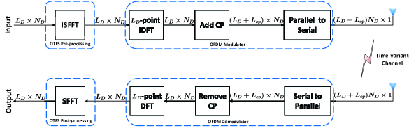
Figure 1: The modulation and demodulation for OTFS.

Murali et al. investigated OTFS modulation for communication over high mobility channels [23]. They utilized the markov chain monte carlo (MCMC) sampling techniques to construct a low complex detection method and a PN pilot sequence based channel estimation scheme in the delay-Doppler domain. In [24], Raviteja et al. proposed embedded pilot-aided channel estimation schemes for OTFS. Raviteja et al. derived the explicit input-output relation and developed one novel low complex message passing algorithm for joint interference cancellation and symbol detection [25]. In [26], Shen et al. proposed a 3D sparse signal model for the DL massive MIMO channel estimation, which was formulated as the sparse signal recovery problem.

In this paper, we apply OTFS for the massive MIMO network. Within the traditional massive MIMO-OFDM, the digital precoders can be placed at different sub-carriers to capture the channel diversity in the frequency domain. Nevertheless, the digital precoders for the massive MIMO-OTFS may happen in the delay-Doppler domain. In this scenario, the base station (BS) should achieve the channel state information (CSI) in the delay-Doppler domain. Moreover, the users also need the corresponding CSI to implement decoding in the delay-Doppler domain. Hence, we will focus on the channel estimation along DL over the massive MIMO-OTFS. Firstly, we introduce the high mobility massive MIMO channel model and the massive MIMO-OTFS scheme. Then, we develop the time domain massive MIMO-OTFS signal model for the UL, where the angle off-grid is considered. The expectation maximization based variational Bayesian (EM-VB) framework is adopted to recover the UL channel parameters including the angles, the delays, the Doppler frequencies, and the channel gains for all scattering paths. To avoid the huge complexity caused by the large matrix inversion, we design the low complex EM-VB to fully exploit the fast Bayesian inference. Thanks to the angle, delay, and Doppler reciprocity between the UL and the DL even in the frequency division duplex (FDD) mode, we can reconstruct the DL parameters including the angles, the delays, and the Doppler frequencies at BS. Furthermore, we examine the DL channel estimation over the delay-Doppler-angle domain. The case, where different scattering paths of any user possess distinguished delay-Doppler signatures, is examined to illustrate the channel dispersion property of the OTFS over the delay-Doppler domain. Under the scenario where all paths of any user are perfectly separated over the angle domain, a effective path scheduling algorithm is proposed to parallel implement the DL 3D channel recovering for the multiple users. For the general case, we utilize the achieved delay-Doppler-angle signatures to construct one least square (LS) estimator with reduced dimension to capture the DL delay-Doppler-angle channels.

The rest of this paper is organized as follows. Section II introduces high mobility massive MIMO channels and describes the massive MIMO-OTFS scheme. In Section III, we extract UL channel parameters with the EM-VB method and construct the low complex EM-VB. In Section IV, we recover the DL channel parameters at BS and analyze the DL massive MIMO channel estimation over the delay-Doppler-angle domain. The simulation results are presented in Section V, and conclusions are drawn in Section VI.

Notations: We use lowercase (uppercase) boldface to denote vector (matrix). $(\cdot)^{T}$, $(\cdot)^{*}$, and $(\cdot)^{H}$ represent the transpose, the complex conjugate and the Hermitian transpose, respectively. $\mathbf{I}_{N}$ represents a $N\times N$ identity matrix. $\mathbf{1}_{N}$ represents a $N\times 1$ all-one vector. $\delta(\cdot)$ is the Dirac delta function. $\mathbb{E}\{\cdot\}$ is the expectation operator. We use $\text{tr}\{\cdot\}$, $\det\{\cdot\}$ and $\text{rank}\{\cdot\}$ to denote the trace, the determinant, and the rank of a matrix, respectively. $[\mathbf{X}]_{ij}$ is the $(i,j)$-th entry of $\mathbf{X}$. $[\mathbf{X}]_{:,\mathcal{Q}}$ (or $[\mathbf{X}]_{\mathcal{Q},:}$) is the submatrix of $\mathbf{X}$ and contains the columns (or rows) with the index set $\mathcal{Q}$. $\mathbf{x}_{\mathcal{Q}}$ is the sub-vector of $\mathbf{x}$ formed by the entries with the index set $\mathcal{Q}$. $|\mathcal{Q}|$ denotes that all elements of the set $\mathcal{Q}$ take their absolute value. $\|\mathcal{Q}\|$ represents the number of elements in the set $\mathcal{Q}$. $\|\mathbf{x}\|$ denotes the modulus of the vector $\mathbf{x}$. $\mathbf{n}\sim\mathcal{CN}(0,\mathbf{I}_{N})$ means that $\mathbf{n}$ is complex circularly-symmetric Gaussian distributed with zero mean and covariance $\mathbf{I}_{N}$. $\lfloor x\rfloor$ denotes the smallest integer no less than $x$, while $\lceil x\rceil$ represents the largest integer no more than $x$. $\backslash$ is the set subtraction operation. $\Re(x)$ is the real component of $x$ and $\Im(x)$ is the image component of $x$. $\text{diag}(\mathbf{X})$ is a column vector formed by the diagonal elements of $\mathbf{X}$.

II System Model

II-A High Mobility Massive MIMO Channel Model

In this work, we consider a single-cell massive MIMO system in the high-mobility scenarios. The BS serves $K$ users who are randomly distributed in the cell. The BS is equipped with a uniform linear array (ULA), which contains $M$ antenna elements and $M\gg K$, and each user is equipped with single antenna. The wireless signal can reach the user side along the line of sight paths or can be reflected by multiple scatterers, which means that the channel links between the BS and the users subject to the frequency-selective fading. Due to the users’ mobility, the channels vary with respect to the time, i.e., the channel links experience the time-selective fading. Along DL, we assume there are $P$ scattering paths, and each scatter path corresponds to one direction of departure (DOD), one Doppler frequency shift, and one time delay. Denote $\theta_{k,p}(r)$ as a DOD for the $p$-th path of user $k$ at time $r$, and the corresponding antenna array spatial steering vector can be defined as:

$$\mathbf{a}(\theta_{k,p}(r))=[1,e^{\jmath 2\pi\frac{d\sin(\theta_{k,p}(r))}{\lambda}},\ldots,e^{\jmath 2\pi(M-1)\frac{d\sin(\theta_{k,p}(r))}{\lambda}}]^{T},$$ (1)

where $d$ is antenna spacing of the BS, and $\lambda$ is the carrier wavelength for DL. Hence, from the geometric channel model, the time-varying DL channels at time $r$ between BS and the user $k$ can be denoted by

$$\mathbf{h}_{k,l}(r)=\sum_{p=1}^{P}{h}_{k,p}e^{\jmath 2\pi\nu_{k,p}rT_{s}}\delta(lT_{s}-\tau_{k,p})\mathbf{a}(\theta_{k,p}(r)),$$ (2)

where $h_{k,p}$, $\tau_{k,p}$ and $\nu_{k,p}$ represent the channel gain, delay and Doppler shift for the $p$-th path of the user $k$, respectively, the index $l$ denotes the index along the delay domain, $r$ represents the time index, $\delta(\cdot)$ denotes the Dirac delta function, and $T_{s}$ is the system sampling period. Furthermore, we suppose that $\tau_{k,p}=r_{1}T_{s}$, where $r_{1}$ is one integer number. However, the $\theta_{k,p}(r)$ keeps relatively constant within a quite long time interval. For example, let us suppose the user moves at the speed of $200$ km/h, and the distance between BS and user is $500$ m. Within $15$ ms, the user can move only $0.83$ m at most. Then the change of DoD seen by the BS is less than $0.1^{\circ}$, which is quite small. Thus, we can omit the time index $r$ of the angle. Obviously, $\mathbf{h}_{k,l}(r)$ can be determined by the $P$ parameter sets $\{\tau_{k,p},\nu_{k,p},\theta_{k,p},h_{k,p}\}_{p=1}^{P}$, and each parameter set corresponds to one propagation path.

II-B Massive MIMO-OTFS Scheme

II-B1 OTFS Modulation

At the $m$-th antenna, a data sequence of length $L_{D}N_{D}$ is rearranged into a two-dimensional data block $\mathbf{X}_{m}\in\mathcal{C}^{L_{D}\times N_{D}}$, where $L_{D}$ and $N_{D}$ are the dimensions of the delay domain and the Doppler domain, respectively. And it is called a two-dimensional OTFS block in the delay-Doppler domain.

First, we apply the inverse symmetric finite Fourier transform (ISFFT) for the pre-processing block and obtain the data block $\tilde{\mathbf{X}}_{m}$ in the time-frequency domain as $\tilde{\mathbf{X}}_{m}=\mathbf{F}_{L_{D}}\mathbf{X}_{m}\mathbf{F}_{N_{D}}^{H}$, where $\mathbf{F}_{L_{D}}\in\mathcal{C}^{L_{D}\times L_{D}}$ and $\mathbf{F}_{N_{D}}\in\mathcal{C}^{N_{D}\times N_{D}}$ are normalized discrete Fourier transform (DFT) matrices, and their entries can be denoted as $[\mathbf{F}_{N_{D}}]_{p,q}=\frac{1}{\sqrt{N_{D}}}e^{-\jmath\frac{2\pi pq}{N_{D}}}$.

Then, taking the $L_{D}$-point inverse DFT (IDFT) on each column of $\tilde{\mathbf{X}}_{m}$, we can obtain the transmitting signal block $\mathbf{S}_{m}\!\in\!\mathcal{C}^{L_{D}\times N_{D}}$ as $\mathbf{S}_{m}\!=\!\mathbf{F}_{L_{D}}^{H}\tilde{\mathbf{X}}_{m}$, where $\mathbf{S}_{m}\!=\!\left[\mathbf{s}_{m,0},\cdots,\mathbf{s}_{m,N_{D}-1}\right]$ and $\mathbf{s}_{m,j}$ represents the $L_{D}\times 1$ vector. Each column of $\mathbf{S}_{m}$ can be regarded as an OFDM symbol. Thus, with respect to one specific delay-Doppler block $\mathbf{X}_{m}$, there are $N_{D}$ OFDM symbols $\{\mathbf{s}_{m,j}\}^{N_{D}-1}_{j=0}$. Moreover, the transmitted signal block $\mathbf{S}_{m}$ can be rewritten as $\mathbf{S}_{m}=\mathbf{X}_{m}\mathbf{F}^{H}_{N_{D}}$.

In order to avoid the inter-symbol interference between blocks, the OFDM modulator usually adds cyclic prefix (CP) for each OFDM symbol $\mathbf{s}_{m,j}$. Therefore, we can obtain the one-dimensional transmitting signal $\mathbf{s}_{m}\in\mathcal{C}^{(L_{D}+L_{cp})N_{D}\times 1}$ over the time domain as $\mathbf{s}_{m}=\text{vec}\{\mathbf{A}_{cp}\mathbf{S}_{m}\}$, where $\mathbf{A}_{cp}=\big{[}[\mathbf{I}_{L_{D}}]_{L_{D}-L_{cp}:L_{D}-1,:}^{T},\mathbf{I}_{L_{D}}^{T}\big{]}^{T}\in\mathcal{C}^{(L_{D}+L_{cp})\times L_{D}}$ is the CP addition matrix, and $L_{cp}$ is the length of CP. Then, $\mathbf{s}_{m}$ occupies bandwidth $L_{D}\bigtriangleup f$ with duration $N_{D}T$, where $\bigtriangleup f$ and $T=(L_{D}+L_{cp})T_{s}$ are the subcarrier spacing and the OFDM symbol period, respectively.

II-B2 OTFS Demodulation

After $\mathbf{s}_{m}$ passing through the time-varying DL channels, user $k$ can receive the $(L_{D}+L_{cp})N_{D}\times 1$ signal vector $\mathbf{z}_{k}$. Firstly, we rearrange $\mathbf{z}_{k}$ as a two-dimensional matrix $\mathbf{Z}_{k}\in\mathcal{C}^{(L_{D}+L_{cp})\times N_{D}}$, i.e., $\mathbf{Z}_{k}=\text{unvec}\{\mathbf{z}_{k}\}$, where each column vector of $\mathbf{Z}_{k}$ can be regarded as one received OFDM symbol with CP. Then, multiplying $\mathbf{Z}_{k}$ with the CP removal matrix $\mathbf{A}_{rcp}=\left[\textbf{0}_{L_{D}\times L_{cp}},\mathbf{I}_{L_{D}}\right]$, we can obtain the OFDM received symbols $\mathbf{A}_{rcp}\mathbf{Z}_{k}$ without CPs. With the $L_{D}$-point DFT on the OFDM received symbols, the received two-dimensional block $\tilde{\mathbf{Y}}_{k}$ in the time-frequency domain can be written as $\tilde{\mathbf{Y}}_{k}=\mathbf{F}_{L_{D}}\mathbf{A}_{rcp}\mathbf{Z}_{k}$.

Finally, with the SFFT operation in post-processing block, $\tilde{\mathbf{Y}}_{k}$ is transformed to the two-dimensional data block $\mathbf{Y}_{k}\in\mathcal{C}^{L_{D}\times N_{D}}$ in the delay-Doppler domain as $\mathbf{Y}_{k}=\mathbf{F}_{L_{D}}^{H}\tilde{\mathbf{Y}}_{k}\mathbf{F}_{N_{D}}$. Then the received two-dimensional block $\tilde{\mathbf{Y}}_{k}$ can be rewritten as $\mathbf{Y}_{k}=\mathbf{A}_{rcp}\mathbf{Z}_{k}\mathbf{F}_{N_{D}}$.

II-B3 Simple Representation of the Received Signal

According to [26], the $(i,j+N_{D}/2)$-th entry of $\mathbf{Y}_{k}$, i.e., $y_{k,i,j+N_{D}/2}$, can be denoted as

$$[\mathbf{Y}_{k}]_{i,j+N_{D}/2}\approx\sum_{m=0}^{M-1}\sum_{i^{\prime}=0}^{L_{D}-1}\!\!\sum_{j^{\prime}=-N_{D}/2}^{N_{D}/2-1}\!\!\!x_{i^{\prime},j^{\prime}+N_{D}/2,m}\tilde{h}_{k,(i-i^{\prime})_{L_{D}},\langle j-j^{\prime}\rangle,m}e^{\jmath 2\pi\frac{i(j-j^{\prime})}{N_{D}(L_{D}+L_{cp})}}\!+\!w_{k,i,j+N_{D}/2},$$ (3)

where $(i\!-\!i^{\prime})_{L_{D}}$ is the remainder after division of $i\!-\!i^{\prime}$ by $L_{D}$, $\langle j\!-\!j^{\prime}\rangle$ denotes $(j\!-\!j^{\prime}\!+\!N_{D}/2)_{N_{D}}\!-\!N_{D}/2$, $x_{i^{\prime},j^{\prime}\!+\!N_{D}/2,m}$ is the $(i^{\prime},j^{\prime}\!+\!N_{D}/2)$-th element of $\mathbf{X}_{m}$, and $\tilde{h}_{k,i,j,m}$ is the equivalent channel over the delay-Doppler-space domain, $i\!=\!0,1,\ldots,L_{D}\!-\!1$, $j\!=\!-N_{D}/2,\ldots,0,\ldots,N_{D}/2\!-\!1$. Here, it is assumed that $w_{k,i,j\!+\!N_{D}/2}$ is complex Gaussian distributed with zero mean and variance $\sigma^{2}$, and is independent from element to element. Moveover, $\tilde{h}_{k,i,j,m}$ can be derived from (2) as

$$\tilde{h}_{k,i,j,m}= \frac{1}{N_{D}}\sum_{n=1}^{N_{D}}\left[\mathbf{h}_{k,i}\left((n-1)(L_{D}+L_{cp})+1\right)\right]_{m}e^{-\jmath 2\pi(n-1)\frac{j}{N_{D}}}$$

$$= \frac{1}{N_{D}}\sum_{p=1}^{P}h_{k,p}e^{\jmath 2\pi\nu_{k,p}T_{s}}\frac{\sin(\pi(\nu_{k,p}N_{D}T-j))}{\sin(\pi\frac{(\nu_{k,p}N_{D}T-j)}{N_{D}})}e^{\jmath\pi\frac{(\nu_{k,p}N_{D}T-j)(N_{D}-1)}{N_{D}}}\delta(iT_{s}-\tau_{k,p})e^{\jmath 2\pi m\frac{d\sin\theta_{k,p}}{\lambda}}.$$ (4)

Similar to [20, 19, 27], we can utilize the spatial DFT operation to dig the channel sparsity caused by the massive antennas. Explicitly, taking the normalized DFT along the antenna index $m$, we can derive the delay-Doppler-angle domain channel $\bar{h}_{k,i,j,q}$ $(q\!=\!-\!\frac{M}{2},\ldots,0,\ldots,\frac{M}{2}\!-\!1)$ as

$$\bar{h}_{k,i,j,q}\triangleq \frac{1}{\sqrt{M}}\sum_{m=0}^{M-1}\tilde{h}_{k,i,j,m}e^{-\jmath 2\pi\frac{qm}{M}},$$

$$= \frac{1}{N_{D}\sqrt{M}}\sum_{p=1}^{P}h_{k,p}e^{\jmath 2\pi\nu_{k,p}T_{s}}\frac{\sin(\pi(\nu_{k,p}N_{D}T-j))}{\sin(\pi\frac{(\nu_{k,p}N_{D}T-j)}{N_{D}})}e^{\jmath\pi\frac{(\nu_{k,p}N_{D}T-j)(N_{D}-1)}{N_{D}}}$$

$$\times\delta(iT_{s}-\tau_{k,p})\frac{\sin(\pi(M\frac{d\sin\theta_{k,p}}{\lambda}-q))}{\sin(\pi\frac{M\frac{d\sin\theta_{k,p}}{\lambda}-q}{M})}e^{\jmath\pi\frac{(M\!\frac{d\sin\theta_{k,p}}{\lambda}-q)(M-1)}{M}}.$$ (5)

From the above equation, it can be checked that $\bar{h}_{k,i,j,q}$ has dominant elements only if $i\approx\tau_{k,p}L_{D}\triangle f$, $j\approx\nu_{k,p}N_{D}T$ and $q\approx M\frac{d\sin\theta_{k,p}}{\lambda}$, and each dominant element corresponds to one specific parameter set $\{\tau_{k,p},\nu_{k,p},\theta_{k,p},h_{k,p}\}$. Thus, there are only $P$ dominant values among $ML_{D}N_{D}$ elements, which means that $\bar{h}_{k,i,j,q}$ is sparse over the delay-Doppler-angle domain as shown in Fig. 2.

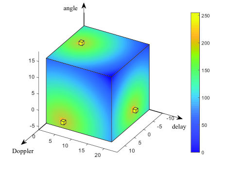
Figure 2: 3D sparse channel over the delay-Doppler-angle domain.

From (3), it can be checked that $x_{i,j,m}$ experiences roughly constant channel $\tilde{h}_{k,i,j,m}$ in the delay-Doppler domain and is affected by the equivalent channel $\tilde{h}_{k,i,j,m}$. Moreover, from (5), it can be found that $\tilde{h}_{k,i,j,m}$ can be equivalently expressed by the sparse delay-Doppler-angle domain channel $\bar{h}_{k,i,j,q}$, which can be determined by the $P$ parameter sets $\{\tau_{k,p},\nu_{k,p},\theta_{k,p},h_{k,p}\}_{p=1}^{P}$. Thus, once we achieve the accurate information about the parameter sets, we can infer $\bar{h}_{k,i,j,q}$. Theoretically, we can achieve $\bar{h}_{k,i,j,q}$ in two ways: One way happens in the time-frequency domain to achieve the $P$ parameter sets, while the other way works in the delay-Doppler-angle domain to directly recover $\bar{h}_{k,i,j,q}$. However, directly recovering $\bar{h}_{k,i,j,q}$ from DL needs powerful sparse signal recovery methods with high computation burden and large training overhead, which is because the non-zero elements among $\bar{h}_{k,i,j,q}$ are unknown. Thus, in the following, we propose UL-aided DL channel estimation framework, which fully exploits the angle, the delay, and the Doppler reciprocity between UL and DL, even in the FDD mode.

III SBL-based Channel Parameter Capturing along UL

Along UL, different users separately send short training sequences to BS, and BS captures the $P$ parameter sets $\{\tau_{k,p}^{ul},\nu_{k,p}^{ul},\theta_{k,p}^{ul},h_{k,p}^{ul}\}_{p=1}^{P}$ for different users in the time-frequency domain, where the superscript “ul” denotes UL variables. Secondly, at BS we try to construct the corresponding DL parameter sets and the related $\bar{h}_{k,i,j,q}$. Meanwhile, we can acquire the exact locations of $P$ nonzero elements in $\bar{h}_{k,i,j,q}$, and send low-overhead training to estimate the $P$ nonzero delay-Doppler-angle domain channels at different users.

III-A UL Transmission Model

With the $P$ parameter sets $\{\tau_{k,p}^{ul},\nu_{k,p}^{ul},\theta_{k,p}^{ul},h_{k,p}^{ul}\}_{p=1}^{P}$, we can define UL channel of the user $k$ as

$$\mathbf{h}_{k,l}^{ul}(r)=\sum_{p=1}^{P}{h}_{k,p}^{ul}e^{\jmath 2\pi\nu^{ul}_{k,p}rT_{s}}\delta(lT_{s}-\tau_{k,p}^{ul})\mathbf{a}^{ul}(\theta_{k,p}^{ul}),$$ (6)

where $\mathbf{a}^{ul}(\theta_{k,p}^{ul})=\bigg{[}1,e^{\jmath 2\pi\frac{d\sin(\theta_{k,p}^{ul})}{\lambda^{ul}}},\ldots,e^{\jmath 2\pi(M-1)\frac{d\sin(\theta_{k,p}^{ul})}{\lambda^{ul}}}\bigg{]}^{T}$ is spatial steering vector corresponding to BS antenna array and $\lambda^{ul}$ is the carrier wavelength for the UL.

During the parameter extraction along UL, each user sends short training sequence to BS. The sequences from different users are orthogonal in the time domain. As shown in Fig. 3, the starting time of the training sequence for user 1 is $n_{1}T_{s}$ and the length of each training is $(L_{cp}+N_{t})T_{s}$, where $n_{1}$ is one integer number, $L_{cp}$ is the length of CP and $N_{t}$ is the number of valid points. The beginning time for the training of the user $k$ is $\left(n_{1}+(L_{cp}+N_{t})(k-1)\right)T_{s}$, $k=1,2,\ldots,K$. Without loss of generality, we assume that each user utilizes the same training $\mathbf{t}_{cp}=[t_{N_{t}-L_{cp}},t_{N_{t}-L_{cp}+1},\dots,t_{N_{t}-1},\mathbf{t}^{T}]^{T}\in\mathcal{C}^{(N_{t}+L_{cp})\times 1}$ along the UL, where $\mathbf{t}=[t_{0},t_{1},\ldots,t_{N_{t}-1}]^{T}$, and $\sigma_{p}^{2}=\|\mathbf{t}\|^{2}$ represents the training power. Then, BS receives the training sequences of the user $k$ within the time interval $[\left(n_{1}+(L_{cp}+N_{t})(k-1)\right)T_{s},$ $\left(n_{1}+(L_{cp}+N_{t})k-1\right)T_{s}]$. It can be checked that the output of the $M$ antennas at the first $L_{cp}$ time samples in this time interval corresponds to the CP part. Hence, we will discard these samples and collect the output of BS’s antennas at time $\left(n_{1}+(L_{cp}+N_{t})(k-1)+L_{cp}+n\right)T_{s}$ into the $M\times 1$ vector $\mathbf{y}_{k,n}^{ul}$, $n=0,1,\ldots,N_{t}-1$.

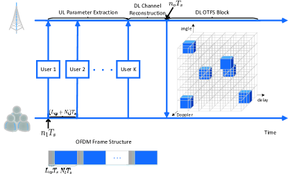
Figure 3: Overall framework in the massive MIMO-OTFS transceiver.

With (6), the received vector $\mathbf{y}_{k,n}^{ul}$ can be denoted as

$$\mathbf{y}_{k,n}^{ul}= \sum_{p=1}^{P}{h}_{k,p}^{ul}e^{\jmath 2\pi\nu^{ul}_{k,p}\left(n_{1}+(L_{cp}+N_{t})(k-1)+L_{cp}+n\right)T_{s}}t_{(n-\tau_{k,p}^{ul}/T_{s})_{N_{t}}}\mathbf{a}^{ul}(\theta_{k,p}^{ul})+\mathbf{v}_{k,n},$$ (7)

where $M\times 1$ vector $\mathbf{v}_{k,n}$ represents the additive white Gaussian noise (AWGN) vector at the $M$ receiving antennas with zero mean and the covariance matrix $\sigma^{2}\mathbf{I}_{M}$. Moreover, $\mathbf{v}_{k,n_{1}}$ is independent on $\mathbf{v}_{k,n_{2}}$, when $n_{1}\neq n_{2}$.

Then, we construct the uniform sampling grids $\{\vartheta_{0},\vartheta_{1},\cdots,\vartheta_{N-1}\}$ and $[0,T_{s},\ldots,(L-1)T_{s}]$ over the angle and delay domain, respectively, where $N$ and $L$ are the number of the angle domain and that of delay domain grids, respectively. Notice that $L$ should be greater than $\tau_{k,p}^{ul}/T_{s}$. With this assumption, we can construct one $N\times L$ sparse matrix $\mathbf{G}_{k}^{ul}$ to map $P$ nonzero channel gains $\{h_{k,p}^{ul}\}_{p=1}^{P}$ onto $N$ angle and $L$ delay grids. If we know the exact information about the $\{\tau_{k,p}^{ul},\nu_{k,p}^{ul},\theta_{k,p}^{ul},h_{k,p}^{ul}\}_{p=1}^{P}$, we can determine the locations of the nonzero entries in $\mathbf{G}_{k}^{ul}$ and their values. For example, if $\{\tau_{k,1}^{ul},\nu_{k,1}^{ul},\theta_{k,1}^{ul},h_{k,1}^{ul}\}$ is available, we find the nearest point with $\tau_{k,1}^{ul}$ among all the delay grids and label its corresponding grid as $l_{1}^{*}T_{s}$. Similarly, the closest point with $\theta_{k,1}^{ul}$ is chosen among all the angle grids and is denoted as $\vartheta_{n_{1}^{*}}$. Then, it can be concluded that $[\mathbf{G}_{k}^{ul}]_{n_{1}^{*},l_{1}^{*}}=h_{k,1}^{ul}$. On the contrary, if all the nonzero elements in $\mathbf{G}_{k}^{ul}$ is found, we can obtain their related channel parameter sets. For example, if $[\mathbf{G}_{k}^{ul}]_{n_{1}^{*},l_{1}^{*}}$ is nonzero, we have $\tau_{k,1}^{ul}=l_{1}^{*}T_{s}$, $\theta_{k,1}=\vartheta_{n_{1}^{*}}$. Moreover, for user $k$, the grid $[0,T_{s},\ldots,(L-1)T_{s}]$ corresponds to $L\times 1$ Doppler shift vector $\boldsymbol{\upsilon}_{k}^{ul}=[\upsilon_{k,0}^{ul},\upsilon_{k,1}^{ul},\ldots,\upsilon_{k,L-1}^{ul}]^{T}$, $k=1,2,\ldots,K$.

Before proceeding, we define $N_{t}\times 1$ vector ${\bf{\text{exp}}}(\upsilon_{k,l}^{ul})$ and $L\times 1$ vector $\boldsymbol{\text{exp}}_{in}(\boldsymbol{\upsilon}_{k}^{ul})$ as

$${\bf{\text{exp}}}(\upsilon_{k,l}^{ul})=[1,e^{\jmath 2\pi\upsilon_{k,l}^{ul}T_{s}},\ldots,e^{\jmath 2\pi\upsilon_{k,l}^{ul}(N_{t}-1)T_{s}}]^{T},$$

$$\boldsymbol{\text{exp}}_{in}(\boldsymbol{\upsilon}_{k}^{ul})=[e^{\jmath 2\pi\upsilon_{k,0}^{ul}(n_{1}+(L_{cp}+N_{t})(k-1)+L_{cp})T_{s}},\ldots,e^{\jmath 2\pi\upsilon_{k,L-1}^{ul}(n_{1}+(L_{cp}+N_{t})(k-1)+L_{cp})T_{s}}]^{T},$$ (8)

where $l\!\!=\!\!0,1,\ldots,L\!-\!1$. Then, we collect $\mathbf{y}_{k,0}^{ul},\ldots,\mathbf{y}_{k,N_{t}\!-\!1}^{ul}$ into the matrix $\mathbf{Y}_{k}^{ul}\!\!=\!\![\mathbf{y}_{k,0}^{ul},\ldots,\mathbf{y}_{k,N_{t}\!-\!1}^{ul}]^{T}$. With $\mathbf{G}_{k}^{ul}$ and taking some mathematical operations in (7), we can denote $\mathbf{Y}_{k}^{ul}$ as

$$\mathbf{Y}_{k}^{ul}= \underbrace{\left[\mathbf{a}^{ul}(\vartheta_{0})\cdots\mathbf{a}^{ul}(\vartheta_{N-1})\right]}_{\mathbf{A}^{ul}}\underbrace{\mathbf{G}_{k}^{ul}\text{diag}(\boldsymbol{\text{exp}}_{in}(\boldsymbol{\upsilon}_{k}^{ul}))}_{\tilde{\mathbf{G}}_{k}^{ul}}\left[\begin{matrix}\boldsymbol{\text{exp}}^{T}(\upsilon_{k,0}^{ul})\odot\left(\mathbf{t}^{T}\mathbf{J}_{0}\right)\\ \vdots\\ \boldsymbol{\text{exp}}^{T}(\upsilon_{k,L-1}^{ul})\odot\left(\mathbf{t}^{T}\mathbf{J}_{L-1}\right)\end{matrix}\right]+\mathbf{V}_{k},$$ (9)

where $\mathbf{J}_{l}\in\mathbb{C}^{N_{t}\times N_{t}}$ is $l$ cyclic shift matrix with first column as the canonical basis vector $\mathbf{e}^{l}_{N_{t}}\!\!=\!\![I_{N_{t}}]_{:,(-l)_{N_{t}}}$, and the $M\!\!\times\!\!N_{t}$ noise matrix $\mathbf{V}_{k}\!\!=\!\![\mathbf{v}_{k,0},\mathbf{v}_{k,1},\ldots,\mathbf{v}_{k,N_{t}-1}]$. Moreover, the $M\!\times\!N$ dictionary matrix $\mathbf{A}^{ul}$ and the equivalent sparse matrix $\tilde{\mathbf{G}}_{k}^{ul}$ have been given in the above equation.

Nonetheless, in the practical system, the Doppler shift is much smaller than the sampling rate $1/T_{s}$. For example, for the system with carrier frequency $6$ GHz, $N_{t}=40$ and $1/T_{s}=20$ MHz, when the user moves at the speed 300 km/h, the maximum phase accumulation within $N_{t}T_{s}$ interval is 0.021, which is much smaller than 1. Thus, we can utilize the Taylor series expansion to approximate ${\bf{\text{exp}}}(\upsilon_{k,l}^{ul})$ as

$${\bf{\text{exp}}}(\upsilon_{k,l}^{ul})\approx\underbrace{\left[1,1+\jmath 2\pi T_{s}\upsilon_{k,l}^{ul},\dots,1+\jmath 2\pi(N_{t}-1)T_{s}\upsilon_{k,l}^{ul}\right]^{T}}_{{\bf{\text{exp}}}_{ap}(\upsilon_{k,l}^{ul})},$$ (10)

where the $N_{t}\times 1$ vector ${\bf{\text{exp}}}_{ap}(\upsilon_{k,l}^{ul})$ is defined. Plugging the above result into (9), we can obtain

$$\mathbf{Y}_{k}^{ul} =\mathbf{A}^{ul}\tilde{\mathbf{G}}_{k}^{ul}\underbrace{\left[\begin{matrix}{\bf{\text{exp}}}_{ap}^{T}(\upsilon_{k,0}^{ul})\odot\left(\mathbf{t}^{T}\mathbf{J}_{0}\right)\\ \vdots\\ {\bf{\text{exp}}}_{ap}^{T}(\upsilon_{k,L-1}^{ul})\odot\left(\mathbf{t}^{T}\mathbf{J}_{L-1}\right)\end{matrix}\right]}_{\mathbf{C}_{k}^{ul}}+\mathbf{V}_{k},$$ (11)

where the $L\times N_{t}$ matrix $\mathbf{C}_{k}^{ul}$ is denoted in the above equation.

As presented in (9), the dictionary $\mathbf{A}^{ul}$ is constructed with the uniform angle grids $\{\vartheta_{0},\dots,\vartheta_{N-1}\}$. Correspondingly, the true DOA set for the $P$ UL scattering pathes is $\{{\theta}_{k,1}^{ul},\dots,\theta_{k,P}^{ul}\}$. In practice, the DOAs may not locate exactly on the predefined spatial grids, and the direction mismatch happens. Under such case, we can approximate the practical steering vector $\mathbf{a}^{ul}(\theta_{k,p}^{ul})$ with the linear expansion as

$$\mathbf{a}^{ul}({{\theta}_{k,i}^{ul}})\approx\mathbf{a}^{ul}(\vartheta_{n_{i}})+\mathbf{b}^{ul}({\vartheta}_{n_{i}})({\theta}_{k,i}^{ul}-\vartheta_{n_{i}}),$$ (12)

where $\vartheta_{n_{i}}$ is the nearest angle grid to the true DOA $\theta_{k,i}^{ul}$, $\mathbf{a}^{ul}(\vartheta_{n_{i}})$ is the steering vector on grid point $\vartheta_{n_{i}}$ and $\mathbf{b}^{ul}({\vartheta}_{n_{i}})$ is derivative of $\mathbf{a}^{ul}(\vartheta_{n_{i}})$ with respect to $\vartheta_{n_{i}}$, i.e., $\mathbf{b}^{ul}({\vartheta}_{n_{i}})=\left(\mathbf{a}^{ul}(\vartheta_{n_{i}})\right)^{\prime}$.

With the off-grid taken into consideration, (11) can be rewritten as

$$\mathbf{Y}_{k}^{ul}=\underbrace{\left(\mathbf{A}^{ul}+\mathbf{B}^{ul}\text{diag}(\boldsymbol{\beta}_{k}^{ul})\right)}_{\tilde{\mathbf{A}}_{k}^{ul}}\tilde{\mathbf{G}}_{k}^{ul}\mathbf{C}_{k}^{ul}+{\mathbf{V}}_{k},$$ (13)

where $\mathbf{B}^{ul}=[\mathbf{b}^{ul}({\vartheta}_{0}),\dots,\mathbf{b}^{ul}({\vartheta}_{N-1})]$, $\boldsymbol{\beta}_{k}^{ul}=[\beta_{k,0}^{ul},\dots,\beta_{k,N-1}^{ul}]^{T}$, and the $M\times N$ matrix $\tilde{\mathbf{A}}_{k}^{ul}$ is given in the above equation. Moreover, it can be assumed that the elements in $\boldsymbol{\beta}_{k}^{ul}$ are independent identical distribution (i.i.d.) according to the uniform distribution within the region $[-\frac{r}{2},\frac{r}{2}]$ , where $r$ is the grid interval for the uniform grid set $\vartheta$, i.e., $r=\vartheta_{n}-\vartheta_{n-1},1\leq n\leq N-1$.

After constructing the observation model (13), we turn the recovering of the $P$ parameter sets $\{\tau_{k,p}^{ul},\nu_{k,p}^{ul},\theta_{k,p}^{ul},h_{k,p}^{ul}\}_{p=1}^{P}$ into the estimation of the sparse matrix $\tilde{\mathbf{G}}_{k}^{ul}$, the basis vector $\boldsymbol{\beta}_{k}^{ul}$, and the corresponding Doppler shift vector $\boldsymbol{\upsilon}_{k}^{ul}=[\upsilon_{k,0}^{ul},\upsilon_{k,1}^{ul},\ldots,\upsilon_{k,L-1}^{ul}]^{T}$. Then, the UL channel parameter extraction can be treated as sparse recovery problem, where the SBL framework can achieve the robust result [28]. Therefore, we will adopt a SBL framework to implement this task in the next subsection.

III-B Probabilistic Models of the SBL Framework

In the following, we will give the detailed probabilistic models for our problem. From (13), we can obtain $\mathbf{y}^{ul}_{k,n}$ as

$$\mathbf{y}^{ul}_{k,n}=\tilde{\mathbf{A}}_{k}^{ul}\tilde{\mathbf{G}}_{k}^{ul}\left[\mathbf{C}_{k}^{ul}\right]_{:,n}+{\mathbf{v}}_{k,n}.$$ (14)

Hence, with the given $\boldsymbol{\beta}_{k}^{ul}$, $\boldsymbol{\upsilon}_{k}^{ul}$, the conditional probability distribution function (PDF) of $\mathbf{y}^{ul}_{k,n}$ on $\tilde{\mathbf{G}}_{k}^{ul}$ can be written as

$$p\left(\mathbf{y}^{ul}_{k,n}|\tilde{\mathbf{G}}_{k}^{ul};\boldsymbol{\beta}_{k}^{ul},\boldsymbol{\upsilon}_{k}^{ul}\right)=\mathcal{CN}\left(\tilde{\mathbf{A}}_{k}^{ul}\tilde{\mathbf{G}}_{k}^{ul}\left[\mathbf{C}_{k}^{ul}\right]_{:,n},\sigma^{2}\mathbf{I}_{M}\right).$$ (15)

Before proceeding, let us define the $NL\times 1$ vector $\mathbf{g}_{k}^{ul}=\text{vec}(\tilde{\mathbf{G}}_{k}^{ul})$. With the property equation $\tilde{\mathbf{A}}_{k}^{ul}\tilde{\mathbf{G}}_{k}^{ul}[\mathbf{C}^{ul}_{k}]_{:,n}=(\left[\mathbf{C}_{k}^{ul}\right]_{:,n}^{T}\otimes\tilde{\mathbf{A}}_{k}^{ul})\text{vec}(\tilde{\mathbf{G}}_{k}^{ul})$ , (14) can be reformulated as

$$\mathbf{y}^{ul}_{k,n}=\boldsymbol{\Phi}_{k,n}\mathbf{g}_{k}^{ul}+{\mathbf{v}}_{k,n},$$ (16)

where $\boldsymbol{\Phi}_{k,n}=\left[\mathbf{C}_{k}^{ul}\right]_{:,n}^{T}\otimes\tilde{\mathbf{A}}_{k}^{ul}\in\mathcal{C}^{M\times NL}$. Let us collect $\mathbf{y}^{ul}_{k,0},\mathbf{y}^{ul}_{k,1},\ldots,\mathbf{y}^{ul}_{k,N_{t}-1}$ into the $N_{t}M\times 1$ vector $\mathbf{y}^{ul}_{k}=[(\mathbf{y}^{ul}_{k,0})^{T},(\mathbf{y}^{ul}_{k,1})^{T},\ldots,(\mathbf{y}^{ul}_{k,N_{t}-1})^{T}]^{T}$ and construct the $N_{t}M\times NL$ matrix $\boldsymbol{\Phi}_{k}=\left[(\boldsymbol{\Phi}_{k,0})^{T},\cdots,(\boldsymbol{\Phi}_{k,N_{t}\!-\!1})^{T}\right]^{T}$ and the $N_{t}M\!\!\times\!\!1$ vector ${\mathbf{v}}_{k}\!\!=\!\!\left[{\mathbf{v}}_{k,0}^{T},\cdots,{\mathbf{v}}_{k,N_{t}\!-\!1}^{T}\right]^{T}$. Then, we can obtain

$$\mathbf{y}^{ul}_{k}=\boldsymbol{\Phi}_{k}\mathbf{g}_{k}^{ul}+{\mathbf{v}}_{k}.$$ (17)

With (15), it can be obtained that

$$p(\mathbf{y}^{ul}_{k}\mid\mathbf{g}_{k}^{ul};\boldsymbol{\beta}_{k}^{ul},\boldsymbol{\upsilon}_{k}^{ul})=\mathcal{CN}\left(\boldsymbol{\Phi}_{k}\mathbf{g}_{k}^{ul},\sigma^{2}\mathbf{I}_{N_{t}M}\right).$$ (18)

Within the SBL framework [29], $\mathbf{g}_{k}^{ul}$ can be hierarchically modeled in Fig. 4, where the squares denote constant variables, the circles represent the hidden variables and the shaded circles correspond to the observations. Here, we set the prior probability of $\mathbf{g}_{k}^{ul}$ as the complex Gaussian distribution with precision matrix $\boldsymbol{\Gamma}_{k}=\text{diag}(\boldsymbol{\alpha_{k}})$, where $\boldsymbol{\alpha}_{k}=\left[\alpha_{k,0},\cdots,\alpha_{k,NL-1}\right]^{T}$. Then, the conditional PDF of $\mathbf{g}_{k}^{ul}$ on $\boldsymbol{\alpha}_{k}$ can be written as

$$p(\mathbf{g}_{k}^{ul}\mid\boldsymbol{\alpha}_{k})=\mathcal{CN}\left(0,\boldsymbol{\Gamma}_{k}^{-1}\right).$$ (19)

Furthermore, $\alpha_{k,i}$ is Gamma distributed as

$$p(\alpha_{k,i})\!=\!\text{Gamma}(\alpha_{k,i}\!\mid\!a_{k},b_{k}),~{}\text{for}\ i\!=\!0,\cdots,NL\!-\!1,$$ (20)

where $\text{Gamma}(\alpha_{k,i}|a_{k},b_{k})\!=\!\frac{b_{k}^{a_{k}}}{\Gamma(a_{k})}\alpha_{k,i}^{a_{k}-1}\text{exp}\{-b_{k}\alpha_{k,i}\}$, $\Gamma(a_{k})$ is the Gamma function, and $a_{k}$ and $b_{k}$ are the constant parameters. If $\alpha_{k,i}$ is Gamma distributed, $p(\alpha_{k,i})$ is the conjugate prior to the the conditional PDF $p([\mathbf{g}_{k}^{ul}]_{i}|\alpha_{k,i})$, which can simplify the calculation of the posterior distribution. Besides, through integrating out the hyperparameter $\alpha_{k,i}$, the marginal distribution of $[\mathbf{g}_{k}^{ul}]_{i}$ is a Student-t distribution [30]. With proper $a_{k}$ and $b_{k}$ in the Gamma distribution, the Student-t distribution is strongly peaked about the origin $[\mathbf{g}_{k}^{ul}]_{i}=0$, which assures the sparsity of $\mathbf{g}_{k}^{ul}$.

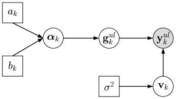
Figure 4: Graphical model for UL channel estimation using SBL.

III-C Solving SBL Using EM-VB

The goal of VB inference is to find a tractable variational distribution $q(\mathcal{H}_{k})$ that closely approximates $p(\mathcal{H}_{k}|\mathbf{y}^{ul}_{k})$ [32], [33]. Here, we denote all hidden variables as $\mathcal{H}_{k}=\{\tilde{\mathbf{G}}_{k}^{ul},\boldsymbol{\alpha}_{k}\}$. Within VB, $q(\mathcal{H}_{k,i})$ can be achieved as

$$q\left(\mathcal{H}_{k,i}\right) \propto\exp\left\{\left\langle\ln p\left(\mathcal{H}_{k},\mathbf{y}^{ul}_{k}\right)\right\rangle_{\sim q\left(\mathcal{H}_{k,i}\right)}\right\},$$ (21)

where $\left\langle\cdot\right\rangle_{\sim q\left(\mathcal{H}_{k,i}\right)}$ denotes the expectation operation with respect to all factors except $q(\mathcal{H}_{k,i})$.

With (21), we can derive the posterior statistics for each variable in $\mathcal{H}_{k}=\{\tilde{\mathbf{G}}_{k}^{ul},\boldsymbol{\alpha}_{k}\}$ through the expectation step of EM-VB and further derive $\{\boldsymbol{\beta}_{k}^{ul},\boldsymbol{\upsilon}_{k}^{ul}\}$ in the maximization step of EM-VB.

III-D Expectation Step of EM-VB

In the expectation phase, we aim to find the approximate posterior distribution of $q(\mathbf{g}_{k}^{ul})$ and $q(\boldsymbol{\alpha}_{k})$. Besides, $\hat{\boldsymbol{\beta}}_{k}^{ul}$ and $\hat{\boldsymbol{\upsilon}}_{k}^{ul}$ obtained from the maximization step are needed to evaluate the estimation of $\boldsymbol{\Phi}_{k}$, i.e., $\hat{\boldsymbol{\Phi}}_{k}$.

III-D1 Estimation of $q(\mathbf{g}_{k}^{ul})$

By applying (18) , (19) and (21), we can obtain $q(\mathbf{g}_{k}^{ul})$ as follows

$$q(\mathbf{g}_{k}^{ul}) \!\varpropto\!\exp\!\left\{\!\ln p(\mathbf{y}^{ul}_{k}|\mathbf{g}_{k}^{ul};\!\hat{\boldsymbol{\beta}}_{k}^{ul},\hat{\boldsymbol{\upsilon}}_{k}^{ul})\!+\!\left\langle\ln p(\mathbf{g}_{k}^{ul}|\boldsymbol{\alpha}_{k})\right\rangle_{q(\boldsymbol{\alpha}_{k})}\right\}$$

$$\varpropto\exp\left\{-(\mathbf{g}_{k}^{ul}-\boldsymbol{\mu}_{k})^{H}\boldsymbol{\Sigma}_{k}^{-1}(\mathbf{g}_{k}^{ul}-\boldsymbol{\mu}_{k})\right\},$$ (22)

where $\mathbf{g}_{k}^{ul}$ is complex Gaussian distributed with the mean and the covariance as

$$\boldsymbol{\mu}_{k}=\frac{1}{\sigma^{2}}\boldsymbol{\Sigma}_{k}\hat{\boldsymbol{\Phi}}_{k}^{H}\mathbf{y}^{ul}_{k},\kern 15.0pt\boldsymbol{\Sigma}_{k}=\left(\frac{1}{\sigma^{2}}\hat{\boldsymbol{\Phi}}_{k}^{H}\hat{\boldsymbol{\Phi}}_{k}+\left\langle\boldsymbol{\Gamma}_{k}\right\rangle_{q(\boldsymbol{\alpha}_{k})}\right)^{-1},$$ (23)

and $\left\langle\mathbf{g}_{k}^{ul}\right\rangle_{q(\mathbf{g}_{k}^{ul})}=\boldsymbol{\mu}_{k}$ can be used for deriving $q(\boldsymbol{\alpha}_{k})$. From (23), we find that in order to obtain $\left\langle\mathbf{g}_{k}^{ul}\right\rangle_{q(\mathbf{g}_{k}^{ul})}$, we need to derive $\left\langle\boldsymbol{\Gamma}_{k}\right\rangle_{q(\boldsymbol{\alpha}_{k})}$ as follows.

III-D2 Estimation of $q(\boldsymbol{\alpha}_{k})$

With (19) and (20), $q(\boldsymbol{\alpha}_{k})$ can be calculated from (21) as

$$q(\boldsymbol{\alpha}_{k}) \varpropto\exp\left\{\left\langle\ln p(\mathbf{g}_{k}^{ul}\mid\boldsymbol{\alpha}_{k})\right\rangle_{q(\mathbf{g}_{k}^{ul})}+\ln p(\boldsymbol{\alpha}_{k})\right\}$$

$$\varpropto\prod_{i=0}^{NL-1}\alpha_{k,i}^{a_{k}+1-1}\exp\!\Big{\{}\!-(b_{k}+\big{\langle}[\mathbf{g}_{k}^{ul}]_{i}^{2}\big{\rangle}_{q(\mathbf{g}_{k}^{ul})})\alpha_{k,i}\!\Big{\}}\!.$$ (24)

Thus, $\alpha_{k,i}$ subjects to $\text{Gamma}(\alpha_{k,i};\widetilde{a}_{k},\widetilde{b}_{k})$, where $\widetilde{a}_{k}=a_{k}+1$ and $\widetilde{b}_{k}=b_{k}+\left\langle\left[\mathbf{g}_{k}^{ul}\right]_{i}^{2}\right\rangle_{q(\mathbf{g}_{k}^{ul})}$. From the property of the Gamma distribution, we can obtain

$$\left\langle\alpha_{k,i}\right\rangle_{q(\boldsymbol{\alpha}_{k})}=\frac{\widetilde{a}_{k}}{\widetilde{b}_{k}}=\frac{a_{k}+1}{b_{k}+\left\langle\left[\mathbf{g}_{k}^{ul}\right]_{i}^{2}\right\rangle_{q(\mathbf{g}_{k}^{ul})}},$$ (25)

where $a_{k}$ and $b_{k}$ can be designed as a reasonable value, and $\left\langle\left[\mathbf{g}_{k}^{ul}\right]_{i}^{2}\right\rangle_{q(\mathbf{g}_{k}^{ul})}$ is the $i$-th element of $\text{diag}(\boldsymbol{\mu}_{k}\boldsymbol{\mu}_{k}^{H}+\boldsymbol{\Sigma}_{k})$. Finally, we can obtain

$$\left\langle\boldsymbol{\Gamma}_{k}\right\rangle_{q(\boldsymbol{\alpha}_{k})}\!=\!\text{diag}\!\Big{(}\!\big{[}\left\langle\alpha_{k,0}\right\rangle_{q(\boldsymbol{\alpha}_{k})}\!,\!\ldots\!,\!\left\langle\alpha_{k,NL-1}\right\rangle_{q(\boldsymbol{\alpha}_{k})}\!\big{]}^{T}\!\Big{)},$$ (26)

which is needed in deriving $\left\langle\mathbf{g}_{k}^{ul}\right\rangle_{q(\mathbf{g}_{k}^{ul})}$.

III-E Maximization Step of EM-VB

With (23) and the definitions of both $\tilde{\mathbf{G}}_{k}^{ul}$ and $\mathbf{g}^{ul}_{k}$, we can achieve $\langle\tilde{\mathbf{G}}_{k}^{ul}\rangle_{q(\mathbf{g}_{k}^{ul})}$ as $\langle\tilde{\mathbf{G}}_{k}^{ul}\rangle_{q(\mathbf{g}_{k}^{ul})}=[[\boldsymbol{\mu}_{k}]_{0:N-1},\cdots,[\boldsymbol{\mu}_{k}]_{(N-1)L:NL-1}]$, which is needed in the derivation of both $\boldsymbol{\beta}_{k}^{ul}$ and $\boldsymbol{\upsilon}_{k}^{ul}$.

III-E1 Computing of $\boldsymbol{\beta}_{k}^{ul}$

In the maximization step of the EM-VB, $\boldsymbol{\beta}_{k}^{ul}$ can be estimated as

$$\hat{\boldsymbol{\beta}}_{k}^{ul}=\max\limits_{\text{diag}(\boldsymbol{\beta}_{k}^{ul})}\left\langle\ln p(\mathbf{Y}_{k}^{ul}\mid\tilde{\mathbf{G}}_{k}^{ul};\boldsymbol{\beta}_{k}^{ul},\boldsymbol{\upsilon}_{k}^{ul})\right\rangle_{q(\mathbf{g}_{k}^{ul})},$$ (27)

which is equivalent to (28) as follows

$$\hat{\boldsymbol{\beta}}_{k}^{ul}=\min\limits_{\boldsymbol{\beta}_{k}^{ul}}\left\langle\bigg{\{}\sum_{n=0}^{N_{t}-1}\frac{1}{\sigma^{2}}\left[\mathbf{y}_{k,n}^{ul}-\mathbf{A}^{ul}\tilde{\mathbf{G}}_{k}^{ul}[\mathbf{C}_{k}^{ul}]_{:,n}-\mathbf{B}^{ul}\text{diag}(\tilde{\mathbf{G}}_{k}^{ul}[\mathbf{C}_{k}^{ul}]_{:,n})\boldsymbol{\beta}_{k}^{ul}\right]^{H}\right.$$

$$\kern 105.0pt\left.\cdot\left[\mathbf{y}_{k,n}^{ul}-\mathbf{A}^{ul}\tilde{\mathbf{G}}_{k}^{ul}[\mathbf{C}_{k}^{ul}]_{:,n}-\mathbf{B}^{ul}\text{diag}(\tilde{\mathbf{G}}_{k}^{ul}[\mathbf{C}_{k}^{ul}]_{:,n})\boldsymbol{\beta}_{k}^{ul}\right]\bigg{\}}\right\rangle_{q(\mathbf{g}_{k}^{ul})}$$ (28)

Taking the derivation of the above equation and let it equal to zero with respect to $\boldsymbol{\beta}_{k}^{ul}$, we have

$$\hat{\boldsymbol{\beta}}_{k}^{ul}=\left[\sum_{n=0}^{N_{t}-1}\Re\left\{\text{diag}\left(\left(\left\langle\tilde{\mathbf{G}}_{k}^{ul}\right\rangle_{q(\mathbf{g}_{k}^{ul})}[\mathbf{C}_{k}^{ul}]_{:,n}\right)^{H}\right)(\mathbf{B}^{ul})^{H}\mathbf{B}^{ul}\text{diag}\left(\left\langle\tilde{\mathbf{G}}_{k}^{ul}\right\rangle_{q(\mathbf{g}_{k}^{ul})}[\mathbf{C}_{k}^{ul}]_{:,n}\right)\right\}\right]^{-1}$$

$$\kern 4.0pt\cdot\sum_{n=0}^{N_{t}-1}\Re\left\{\text{diag}\left(\left(\left\langle\tilde{\mathbf{G}}_{k}^{ul}\right\rangle_{q(\mathbf{g}_{k}^{ul})}[\mathbf{C}_{k}^{ul}]_{:,n}\right)^{H}\right)(\mathbf{B}^{ul})^{H}\left(\mathbf{y}_{k,n}^{ul}-\mathbf{A}^{ul}\left\langle\tilde{\mathbf{G}}_{k}^{ul}\right\rangle_{q(\mathbf{g}_{k}^{ul})}[\mathbf{C}_{k}^{ul}]_{:,n}\right)\right\}.$$ (29)

III-E2 Computing of $\boldsymbol{\upsilon}_{k}^{ul}$

Let us define the $L\times N_{t}$ matrix $\mathbf{D}_{k}=\left[(\mathbf{t}^{T}\mathbf{J}_{0})^{T},\cdots,(\mathbf{t}^{T}\mathbf{J}_{L-1})^{T}\right]^{T}$. Then, we can obtain $\mathbf{C}_{k}^{ul}=\left[{\bf{\text{exp}}}_{ap}(\upsilon_{k,0}^{ul}),\ldots,{\bf{\text{exp}}}_{ap}(\upsilon_{k,L-1}^{ul})\right]^{T}\odot\mathbf{D}_{k}$ and $[\mathbf{C}_{k}^{ul}]_{:,n}=\text{diag}([\mathbf{D}_{k}]_{:,n})\times\left(\mathbf{1}_{L}+\jmath 2\pi nT_{s}\boldsymbol{\upsilon}_{k}^{ul}\right)$.

Then the estimations of $\boldsymbol{\upsilon}_{k}^{ul}$ can be given by

$$\hat{\boldsymbol{\upsilon}}_{k}^{ul}=\max\limits_{\boldsymbol{\upsilon}_{k}^{ul}}\left\langle\sum_{n=0}^{N_{t}-1}\ln p(\mathbf{y}_{k,n}^{ul}\mid\tilde{\mathbf{G}}_{k}^{ul};\boldsymbol{\beta}_{k}^{ul},\boldsymbol{\upsilon}_{k}^{ul})\right\rangle_{q(\mathbf{g}_{k}^{ul})},$$ (30)

which is equivalent to (31) as follows

$$\hat{\boldsymbol{\upsilon}}_{k}^{ul}=\!\min\limits_{\boldsymbol{\upsilon}_{k}^{ul}}\left\langle\!\sum_{n=0}^{N_{t}-1}\!\bigg{\{}\!\left[\mathbf{y}_{k,n}^{ul}\!\!-\!\tilde{\mathbf{A}}_{k}^{ul}\tilde{\mathbf{G}}_{k}^{ul}\text{diag}([\mathbf{D}_{k}]_{:,n})\!\left(\mathbf{1}_{L}\!\!+\!\jmath 2\pi nT_{s}\boldsymbol{\upsilon}_{k}^{ul}\right)\!\right]^{H}\!\!\right.$$

$$\left.\kern 120.0pt\cdot\!\left[\mathbf{y}_{k,n}^{ul}\!\!-\!\!\tilde{\mathbf{A}}_{k}^{ul}\tilde{\mathbf{G}}_{k}^{ul}\text{diag}([\mathbf{D}_{k}]_{:,n})\!\left(\mathbf{1}_{L}\!\!+\!\jmath 2\pi nT_{s}\boldsymbol{\upsilon}_{k}^{ul}\right)\!\right]\!\bigg{\}}\!\right\rangle_{q(\mathbf{g}_{k}^{ul})}$$

$$\kern 15.0pt=\min\limits_{\boldsymbol{\upsilon}_{k}^{ul}}\left\langle\sum_{n=0}^{N_{t}-1}\bigg{\{}\Big{[}(2\pi nT_{s})^{2}(\boldsymbol{\upsilon}_{k}^{ul})^{H}\text{diag}([\mathbf{D}_{k}]_{:,n}^{H})(\tilde{\mathbf{G}}_{k}^{ul})^{H}(\tilde{\mathbf{A}}_{k}^{ul})^{H}\tilde{\mathbf{A}}_{k}^{ul}\tilde{\mathbf{G}}_{k}^{ul}\text{diag}([\mathbf{D}_{k}]_{:,n})\boldsymbol{\upsilon}_{k}^{ul}\right.$$

$$\kern 120.0pt\left.-(\jmath 2\pi nT_{s})(\mathbf{O}_{k,n}^{ul})^{H}\tilde{\mathbf{A}}_{k}^{ul}\tilde{\mathbf{G}}_{k}^{ul}\text{diag}([\mathbf{D}_{k}]_{:,n})\boldsymbol{\upsilon}_{k}^{ul}\right.$$

$$\left.\kern 120.0pt+(\jmath 2\pi nT_{s})(\boldsymbol{\upsilon}_{k}^{ul})^{H}\text{diag}([\mathbf{D}_{k}]_{:,n}^{H})(\tilde{\mathbf{G}}_{k}^{ul})^{H}(\tilde{\mathbf{A}}_{k}^{ul})^{H}\mathbf{O}_{k,n}^{ul}\Big{]}\bigg{\}}\right\rangle_{q(\mathbf{g}_{k}^{ul})},$$ (31)

and $\mathbf{O}_{k,n}^{ul}=\mathbf{y}_{k,n}^{ul}-\tilde{\mathbf{A}}_{k}^{ul}\tilde{\mathbf{G}}_{k}^{ul}\text{diag}([\mathbf{D}_{k}]_{:,n})\mathbf{1}_{L}$ in (31).

With the similar operations in deriving $\hat{\boldsymbol{\beta}}_{k}^{ul}$, we can obtain

$$\hat{\boldsymbol{\upsilon}}_{k}^{ul}=\boldsymbol{\Pi}_{k}^{-1}\boldsymbol{\omega}_{k},$$ (32)

where

$$\boldsymbol{\Pi}_{k}= \sum_{n=0}^{N_{t}-1}(2\pi nT_{s})\Re\left\{\text{diag}([\mathbf{D}_{k}]_{:,n}^{H})\left\langle\tilde{\mathbf{G}}_{k}^{ul}\right\rangle_{q(\mathbf{g}_{k}^{ul})}^{H}(\tilde{\mathbf{A}}_{k}^{ul})^{H}\tilde{\mathbf{A}}_{k}^{ul}\left\langle\tilde{\mathbf{G}}_{k}^{ul}\right\rangle_{q(\mathbf{g}_{k}^{ul})}\text{diag}([\mathbf{D}_{k}]_{:,n})\right\},$$

and

$$\boldsymbol{\omega}_{k}= \sum_{n=0}^{N_{t}-1}\Im\left\{\text{diag}([\mathbf{D}_{k}]_{:,n}^{H})\left\langle\tilde{\mathbf{G}}_{k}^{ul}\right\rangle_{q(\mathbf{g}_{k}^{ul})}^{H}(\tilde{\mathbf{A}}_{k}^{ul})^{H}\!\left(\!\mathbf{y}_{k,n}^{ul}\!-\!\tilde{\mathbf{A}}_{k}^{ul}\left\langle\tilde{\mathbf{G}}_{k}^{ul}\right\rangle_{q(\mathbf{g}_{k}^{ul})}\text{diag}([\mathbf{D}_{k}]_{:,n})\mathbf{1}_{L}\!\right)\!\right\}.$$

With $\{\hat{\boldsymbol{\beta}}_{k}^{ul},\hat{\boldsymbol{\upsilon}}_{k}^{ul}\}$ in the maximization step, we can update $q(\mathbf{g}_{k}^{ul})$ and $q(\boldsymbol{\alpha}_{k})$ to approximate $p\left(\mathbf{g}_{k}^{ul}|\mathbf{y}^{ul}_{k}\right)$ and $p\left(\boldsymbol{\alpha}_{k}|\mathbf{y}^{ul}_{k}\right)$ in (22) and (24), respectively. Furthermore, with $q(\mathbf{g}_{k}^{ul})$ given in the expectation step, we can separately obtain the estimation of $\boldsymbol{\beta}_{k}^{ul}$ and $\boldsymbol{\upsilon}_{k}^{ul}$ in (29), (32) during the maximization step. Iteratively implementing both the expectation and the maximization steps, we can separately obtain the estimation of $\mathbf{g}_{k}^{ul}$ as $\hat{\mathbf{g}}_{k}^{ul}=\left\langle\mathbf{g}_{k}^{ul}\right\rangle_{q(\mathbf{g}_{k}^{ul})}$. Correspondingly, the EM-VB scheme is summarized in Algorithm 1.

Algorithm 1 UL parameter extraction of user $k$ with EM-VB scheme

1:  Input: Training vector $\mathbf{t}$, hyper-parameters in $\{a_{k},b_{k}\}$.

2:  Initialize: $N_{maxiter}$ and the unknown vector set $\{\boldsymbol{\beta}_{k}^{ul},\boldsymbol{\upsilon}_{k}^{ul}\}$.

3:  while $l^{EM}<N_{maxiter}$ do

4:     $l^{EM}=1$.

5:     E-step:

6:       Update $\mathbf{g}_{k}^{ul}$ by (23).

7:       Update $\boldsymbol{\alpha}_{k}$ by (25).

8:     M-step:

9:       Update $\boldsymbol{\beta}_{k}^{ul}$ by (29).

10:       Update $\boldsymbol{\upsilon}_{k}^{ul}$ by (32).

11:     $l^{EM}\leftarrow l^{EM}+1$.

12:  end while

13:  return  $\mathbf{g}^{ul}_{k}$, $\boldsymbol{\beta}_{k}^{ul}$ and $\boldsymbol{\upsilon}_{k}^{ul}$.

III-F Low Complex EM-VB

The EM-VB in the previous subsection is mathematically reasonable and efficient. However, it can be seen from (23) that EM-VB requires the inversion of $NL\times NL$ matrix at each iteration step. In order to overcome this bottleneck, we will resort to the fast Bayesian inference to design the low complex EM-VB, which also contains the expectation and the maximization steps [31]. Explicitly, within the expectation step, $\boldsymbol{\alpha}_{k}$ can be recovered through the maximum a posteriori (MAP) estimator as

$$\hat{\boldsymbol{\alpha}}_{k}=\max\limits_{{\boldsymbol{\alpha}}_{k}}\mathcal{L}(\boldsymbol{\alpha}_{k}),\textit{s.t.}~{}\alpha>0,$$ (33)

where

$$\mathcal{L}(\boldsymbol{\alpha}_{k})= \log p(\mathbf{y}_{k}^{ul}\mid\boldsymbol{\alpha}_{k};\hat{\boldsymbol{\beta}}_{k}^{ul},\hat{\boldsymbol{\upsilon}}_{k}^{ul})$$

$$= \!-\!\big{[}MN_{t}\log\pi\!+\!\log|\underbrace{\sigma^{2}\mathbf{I}_{MN_{t}}\!+\!\hat{\boldsymbol{\Phi}}_{k}\boldsymbol{\Gamma}^{-1}\hat{\boldsymbol{\Phi}}_{k}^{H}}_{\boldsymbol{\Xi}_{k}}|\!+\!(\mathbf{y}_{k}^{ul})^{H}(\sigma^{2}\mathbf{I}_{MN_{t}}\!+\!\hat{\boldsymbol{\Phi}}_{k}\boldsymbol{\Gamma}^{-1}\hat{\boldsymbol{\Phi}}_{k}^{H})^{-1}\mathbf{y}_{k}^{ul}\big{]},$$ (34)

and $\boldsymbol{\Xi}_{k}$ is presented in the above equation. Moreover, instead of deriving all the elements of $\boldsymbol{\alpha}_{k}$ in (24) within each expectation step of the EM-VB, only one entry in $\boldsymbol{\alpha}_{k}$ would be updated in each iteration of the fast Bayesian inference.

Before proceeding, we give the following matrix properties. From the matrix theory, $\boldsymbol{\Xi}_{k}$ in (34) can be rewritten as

$$\boldsymbol{\Xi}_{k} =\sigma^{2}\mathbf{I}_{MN_{t}}+\sum_{j\neq i}\alpha_{k,j}^{-1}[\hat{\boldsymbol{\Phi}}_{k}]_{:,j}[\hat{\boldsymbol{\Phi}}_{k}]_{:,j}^{H}+\alpha_{k,i}^{-1}[\hat{\boldsymbol{\Phi}}_{k}]_{:,i}[\hat{\boldsymbol{\Phi}}_{k}]_{:,i}^{H}$$

$$=\boldsymbol{\Xi}_{k,-i}+\alpha_{k,i}^{-1}[\hat{\boldsymbol{\Phi}}_{k}]_{:,i}[\hat{\boldsymbol{\Phi}}_{k}]_{:,i}^{H},$$ (35)

where $\boldsymbol{\Xi}_{k,-i}$ contains all items of $\boldsymbol{\Xi}_{k}$ without the items related to $\alpha_{k,i}$. With the matrix inversion lemma and the determinant property, we can obtain

$$\boldsymbol{\Xi}_{k}^{-1}=\boldsymbol{\Xi}_{k,-i}^{-1}-\frac{\boldsymbol{\Xi}_{k,-i}^{-1}[\hat{\boldsymbol{\Phi}}_{k}]_{:,i}[\hat{\boldsymbol{\Phi}}_{k}]_{:,i}^{H}\boldsymbol{\Xi}_{k,-i}^{-1}}{\alpha_{k,i}+[\hat{\boldsymbol{\Phi}}_{k}]_{:,i}^{H}\boldsymbol{\Xi}_{k,-i}^{-1}[\hat{\boldsymbol{\Phi}}_{k}]_{:,i}},$$

$$|\boldsymbol{\Xi}_{k}|=|\boldsymbol{\Xi}_{k,-i}||1+\alpha_{k,i}^{-1}[\hat{\boldsymbol{\Phi}}_{k}]_{:,i}^{H}\boldsymbol{\Xi}_{k,-i}^{-1}[\hat{\boldsymbol{\Phi}}_{k}]_{:,i}|.$$ (36)

Since only $\alpha_{k,i}$ needs to be updated with the other elements of $\boldsymbol{\alpha}_{k}$ unchanging, we can decompose the $\mathcal{L}(\boldsymbol{\alpha}_{k})$ as

$$\mathcal{L}(\boldsymbol{\alpha}_{k})= \mathcal{L}(\boldsymbol{\alpha}_{k,-i})\!+\!\log\alpha_{k,i}\!-\!\log(\alpha_{k,i}\!+\!\underbrace{[\hat{\boldsymbol{\Phi}}_{k}]_{:,i}^{H}\boldsymbol{\Xi}_{k,-i}^{-1}[\hat{\boldsymbol{\Phi}}_{k}]_{:,i}}_{p_{k,i}})+\frac{\Big{(}\overbrace{\|[\hat{\boldsymbol{\Phi}}_{k}]_{:,i}^{H}\boldsymbol{\Xi}_{k,-i}^{-1}\mathbf{y}_{k}^{ul}\|}^{q_{k,i}}\Big{)}^{2}}{\alpha_{k,i}+[\hat{\boldsymbol{\Phi}}_{k}]_{:,i}^{H}\boldsymbol{\Xi}_{k,-i}^{-1}[\hat{\boldsymbol{\Phi}}_{k}]_{:,i}}$$

$$= \mathcal{L}(\boldsymbol{\alpha}_{k,-i})+\ell(\alpha_{k,i}),$$ (37)

where $\ell(\alpha_{k,i})=\log\alpha_{k,i}-\log(\alpha_{k,i}+p_{k,i})+\frac{q_{k,i}^{2}}{\alpha_{k,i}+p_{k,i}}$, $\mathcal{L}(\boldsymbol{\alpha}_{k,-i})$ is one function of the $(NL-1)\times 1$ vector $\boldsymbol{\alpha}_{k,-i}=[\alpha_{k,0},\ldots,\alpha_{k,i-1},\alpha_{k,i+1},\ldots,\alpha_{k,NL-1}]^{T}$, and the terms $p_{k,i}$ and $q_{k,i}$ are defined in the above equations. Notice that $\mathcal{L}(\boldsymbol{\alpha}_{k,-i})$, $p_{k,i}$ and $q_{k,i}$ do not depend on $\alpha_{k,i}$. Moreover, (36) is utilized in the above derivation.

Then, with (33) and (37), for fixed $\boldsymbol{\alpha}_{k,-i}$, $\alpha_{k,i}$ can be estimated as

$$\hat{\alpha}_{k,i}=\max_{\alpha_{k,i}}\ell(\alpha_{k,i}),\textit{s.t.}~{}\alpha_{k,i}>0.$$ (38)

Taking the derivative of $\ell(\alpha_{k,i})$ with respect to $\alpha_{k,i}$, we have

$$\frac{d\ell(\alpha_{k,i})}{d\alpha_{k,i}}=\frac{1}{\alpha_{k,i}}-\frac{1}{\alpha_{k,i}+p_{k,i}}-\frac{q_{k,i}^{2}}{(\alpha_{k,i}+p_{k,i})^{2}}.$$ (39)

With fixed $\boldsymbol{\alpha}_{k,-i}$, $\alpha_{k,i}$ can be updated as

$$\alpha_{k,i}=\left\{\begin{aligned} \frac{p_{k,i}^{2}}{q_{k,i}^{2}-p_{k,i}},\kern 45.0pt\text{if}\ q_{k,i}^{2}>p_{k,i},\\ \infty,\kern 82.0pt\text{if}\ q_{k,i}^{2}\leqslant p_{k,i}.\end{aligned}\right.$$

Interestingly, $\alpha_{k,i}=\infty$ means that the variance of $[\mathbf{h}_{k}^{ul}]_{i}$ is 0, and the column vector $[\hat{\boldsymbol{\Phi}}_{k}]_{:,i}$ has no contribution to the observation vector $\mathbf{y}_{k}^{ul}$. Hence, we can prune the basis $[\hat{\boldsymbol{\Phi}}_{k}]_{:,i}$ out of the observation signal space, which can effectively decrease the problem dimension.

Iteratively implementing the above steps from $\alpha_{k,0}$ to $\alpha_{k,NL-1}$, we can obtain the effective signal observation space $\mathcal{B}=\{[\hat{\boldsymbol{\Phi}}_{k}]_{:,i}|\alpha_{k,i}\neq\infty\}$, and collect all the column vectors in $\mathcal{B}$ to form the matrix $\boldsymbol{\widehat{\Phi}}_{k}^{e}$. To clearly illustrate the updating process of $\boldsymbol{\alpha}_{k}$, we use the superscript $(l)$ to represent the variables in the $l$-th iteration. According to the status of both $\alpha_{k,i}^{(l-1)}$ and $\mathcal{B}^{(l-1)}$, we have three operations in current $l$-th iteration. For $\alpha_{k,i}^{(l-1)}<\infty$ and $[q_{k,i}^{(l-1)}]^{2}>p^{(l-1)}_{k,i}$, which means that $[\hat{\boldsymbol{\Phi}}_{k}]_{:,i}$ belongs to $\mathcal{B}^{(l-1)}$ within the $(l-1)$-th iteration , we have $\mathcal{B}^{(l)}=\mathcal{B}^{(l-1)}$ and re-estimate $\alpha_{k,i}^{(l)}$ as $\frac{\left[p^{(l-1)}_{k,i}\right]^{2}}{\left[q_{k,i}^{(l-1)}\right]^{2}-p^{(l-1)}_{k,i}}$. For $\alpha_{k,i}^{(l-1)}=\infty$ and $[q_{k,i}^{(l-1)}]^{2}>p^{(l-1)}_{k,i}$, which corresponds to the case that $[\hat{\boldsymbol{\Phi}}_{k}]_{:,i}$ does not lie in $\mathcal{B}^{(l-1)}$, we should add $[\hat{\boldsymbol{\Phi}}_{k}]_{:,i}$ into $\mathcal{B}^{(l)}$, i.e., $\mathcal{B}^{(l)}=\{\mathcal{B}^{(l-1)},[\hat{\boldsymbol{\Phi}}_{k}]_{:,i}\}$, and update $\alpha_{k,i}^{(l)}$ as $\frac{\left[p^{(l-1)}_{k,i}\right]^{2}}{\left[q_{k,i}^{(l-1)}\right]^{2}-p^{(l-1)}_{k,i}}$. If $\alpha_{k,i}^{(l-1)}<\infty$ and $[q_{k,i}^{(l-1)}]^{2}\leq p^{(l-1)}_{k,i}$, we can verify that $[\hat{\boldsymbol{\Phi}}_{k}]_{:,i}$ lies in $\mathcal{B}^{(l-1)}$ but should not be put into $\mathcal{B}^{(l)}$. So, we prune $\{[\hat{\boldsymbol{\Phi}}_{k}]_{:,i}\}$ out of $\mathcal{B}^{(l-1)}$ to obtain $\mathcal{B}^{(l)}=\mathcal{B}^{(l-1)}\backslash\{[\hat{\boldsymbol{\Phi}}_{k}]_{:,i}\}$ and set $\alpha^{(l)}_{k,i}$ as $\infty$.

With the similar methods in [34] and (37), the term $q_{k,i}^{(l)}$ and $p^{(l)}_{k,i}$ can be achieved from the following equations

$$p_{k,i}^{(l)} =\frac{\alpha_{k,i}^{(l)}P_{k,i}^{(l)}}{\alpha_{k,i}^{(l)}-P_{k,i}^{(l)}},\kern 30.0ptq_{k,i}^{(l)}=\frac{\alpha_{k,i}^{(l)}Q_{k,i}^{(l)}}{\alpha_{k,i}^{(l)}-P_{k,i}^{(l)}},$$ (40)

$$P_{k,i}^{(l)} =\sigma^{-2}[\hat{\boldsymbol{\Phi}}_{k}]_{:,i}^{H}[\widehat{\boldsymbol{\Phi}}_{k}]_{:,i}-\sigma^{-4}[\hat{\boldsymbol{\Phi}}_{k}]_{:,i}^{H}\widehat{\boldsymbol{\Phi}}_{k}^{e,(l)}\boldsymbol{\Sigma}_{k}^{e,(l)}(\widehat{\boldsymbol{\Phi}}_{k}^{e,(l)})^{H}[\hat{\boldsymbol{\Phi}}_{k}]_{:,i},$$ (41)

$$Q_{k,i}^{(l)} =\sigma^{-2}[\hat{\boldsymbol{\Phi}}_{k}]_{:,i}^{H}\mathbf{y}_{k}^{ul}-\sigma^{-4}[\hat{\boldsymbol{\Phi}}_{k}]_{:,i}^{H}\widehat{\boldsymbol{\Phi}}_{k}^{e,(l)}\boldsymbol{\Sigma}_{k}^{e,(l)}(\widehat{\boldsymbol{\Phi}}_{k}^{e,(l)})^{H}\mathbf{y}_{k}^{ul},$$ (42)

where $\widehat{\boldsymbol{\Phi}}_{k}^{e,(l)}$ corresponds to $\mathcal{B}^{(l)}$. $\boldsymbol{\mu}_{k}^{e,(l)}$ and $\boldsymbol{\Sigma}_{k}^{e,(l)}$ can be defined from (23) as

$$\boldsymbol{\mu}_{k}^{e,(l)} =\frac{1}{\sigma^{2}}\boldsymbol{\Sigma}_{k}^{e,(l)}(\widehat{\boldsymbol{\Phi}}_{k}^{e,(l)})^{H}\mathbf{y}^{ul}_{k},$$ (43)

$$\boldsymbol{\Sigma}_{k}^{e,(l)} =\left(\frac{1}{\sigma^{2}}(\widehat{\boldsymbol{\Phi}}_{k}^{e,(l)})^{H}\widehat{\boldsymbol{\Phi}}_{k}^{e,(l)}+\boldsymbol{\Gamma}_{k}^{e,(l)}\right)^{-1},$$ (44)

and $\boldsymbol{\Gamma}_{k}^{e,(l)}$ is constructed from the diagonal matrix $\text{diag}\big{\{}\alpha_{k,0}^{(l)},\alpha_{k,1}^{(l)},\ldots,\alpha_{k,NL-1}^{(l)}\big{\}}$ through deleting the diagonal elements with value of $\infty$. It can be checked that $\widehat{\boldsymbol{\Phi}}_{k}^{e,(l)}$, $\mathcal{B}^{(l)}$, and $\boldsymbol{\Sigma}_{k}^{e,(l)}$ only correspond to the non-zero positions in the sparse vector $\mathbf{h}_{k}^{(ul)}$. Hence, the inversion operation in (44) would be much simpler than that in (23). Fortunately, when only one element in $\boldsymbol{\alpha}_{k}$ is updated at each iteration, $\boldsymbol{\Sigma}_{k}^{e,(l)}$ can be sequentially derived from $\boldsymbol{\Sigma}_{k}^{e,(l-1)}$, whose details can be found in the appendix of [34].

Notice that the fast Bayesian inference just modify the recovering of $\boldsymbol{\alpha}_{k}$ in expectation step of EM-VB. Correspondingly, we summarize the low complex EM-VB in Algorithm 2.

III-G Complexity Analysis

For the VB method, the computational complexity mainly depends on the calculation of the matrix inverse $\boldsymbol{\Sigma}_{k}$ in (23), where a computational complexity in the order of $\mathcal{O}(N^{3}L^{3})$ is required.

Due to the high computational complexity, we resort to the fast VB method to overcome this bottleneck. The computational complexity can be reduced to $\mathcal{O}(M^{3}N_{t}^{3})$, which is due to the fact that $MN_{t}<NL$. Moreover, in the fast VB method, a single $\alpha_{k,i}$ will be updated at each iteration instead of updating the whole $\alpha_{k,i},i\in\{0,1,\ldots,NL-1\}$, which leads to very efficient updates of the mean $\boldsymbol{\mu}_{k}^{e,(l)}$ and the covariance matrix $\boldsymbol{\Sigma}_{k}^{e,(l)}$ in (43) and (44), respectively. Because $\mathbf{g}^{ul}_{k}$ is highly sparse, $\boldsymbol{\Sigma}_{k}$ can be constructed with fewer dimensions than $NL\times NL$, which further reduces the computational complexity.

Algorithm 2 UL parameter extraction of user $k$ with fast variational Bayesian procedure

1:  Input: Training vector $\mathbf{t}$, hyper-parameters in $\{a_{k},b_{k}\}$.

2:  Initialize: $N_{maxiter}$ and the unknown vector set $\{\boldsymbol{\beta}_{k}^{ul},\boldsymbol{\upsilon}_{k}^{ul}\}$.

3:  while $l^{EM}<N_{maxiter}$ do

4:     $l^{EM}=1$.

5:     E-step:

6:     while convergence criterion not met  do

7:        $l=1$.

8:        Choose a $\alpha_{k,i}^{(l-1)}$ (or equivalently choose a basis vector $[\hat{\boldsymbol{\Phi}}_{k}]_{:,i}$).

9:        if $(q_{k,i}^{(l-1)})^{2}>p_{k,i}^{(l-1)}$ $\&$ $\alpha_{k,i}^{(l-1)}=\infty$ then

10:           add $\alpha_{k,i}^{(l)}$ to the model.

11:        else if $(q_{k,i}^{(l-1)})^{2}>p_{k,i}^{(l-1)}$ $\&$ $\alpha_{k,i}^{(l-1)}\neq\infty$ then

12:           re-estimate $\alpha_{k,i}^{(l)}$.

13:        else if $(q_{k,i}^{(l-1)})^{2}<p_{k,i}^{(l-1)}$ then

14:           prune $i$ from the model (set $\alpha_{k,i}^{(l)}=\infty$).

15:        end if

16:        Update $\boldsymbol{\mu}_{k}^{e,(l)}$ and $\boldsymbol{\Sigma}_{k}^{e,(l)}$.

17:        Update $p_{k,i}^{(l)}$ and $q_{k,i}^{(l)}$.

18:        $l\leftarrow l+1$.

19:     end while

20:     Update $\mathbf{g}_{k}^{ul}$ by (23).

21:     M-step:

22:     Update $\boldsymbol{\beta}_{k}^{ul}$ by (29).

23:     Update $\boldsymbol{\upsilon}_{k}^{ul}$ by (32).

24:     $l^{EM}\leftarrow l^{EM}+1$.

25:  end while

26:  return  $\mathbf{g}^{ul}_{k}$, $\boldsymbol{\beta}_{k}^{ul}$ and $\boldsymbol{\upsilon}_{k}^{ul}$.

IV Effective Downlink Channel Reconstruction and Estimation over Delay-Doppler-Angle Domain

IV-A DL Channel Reconstruction at BS

Within $[(n_{1}+(L_{cp}+N_{t})(k-1))T_{s},(n_{1}+(L_{cp}+N_{t})k-1)T_{s}]$, each user captures its UL channel parameter sets through achieving $\{\hat{\tilde{\mathbf{G}}}_{k}^{ul}$, $\hat{\boldsymbol{\beta}}_{k}^{ul}$, $\hat{\boldsymbol{\upsilon}}_{k}^{ul}\}$. However, as shown in Fig. 3, the OTFS-based transmission happens along DL within the interval $[n_{o}T_{s},n_{o}T_{s}+(L_{D}+L_{cp})N_{D}]$. Thus, we should utilize UL channel characteristics seen by BS within the interval $[(n_{1}+(L_{cp}+N_{t})(k-1))T_{s},(n_{1}+(L_{cp}+N_{t})k-1)T_{s}]$ to infer the time-varying trajectory of the DL channels during the OTFS transmission. Thanks to the geometric propagation model in (2) and (6), and we can complete this task according to the following steps.

Firstly, we utilize the sparse channel gain matrix $\hat{\tilde{\mathbf{G}}}_{k}^{ul}$, the Doppler shift vector $\hat{\boldsymbol{\upsilon}}_{k}^{ul}$ and the angle basis vector $\hat{\boldsymbol{\beta}}_{k}^{ul}$ to achieve the estimations of the $P$ UL parameter sets, i.e., $\{{\tau}_{k,p}^{ul},\!{\nu}_{k,p}^{ul},\!{\theta}_{k,p}^{ul},\!{h}_{k,p}^{ul}\}_{p=1}^{P}$. Secondly, the obtained UL parameter sets are utilized to construct the DL channel parameter sets, i.e., $\{{\tau}_{k,p},{\nu}_{k,p},{\theta}_{k,p},{h}_{k,p}\}_{p=1}^{P}$, which will be resorted to construct the delay-Doppler-angle domain channel $\bar{h}_{k,i,j,q}$ in the third step.

For the first step, as the channel gain matrix $\hat{\tilde{\mathbf{G}}}_{k}^{ul}$ is sparse, we can extract several non-zero points of $\hat{\tilde{\mathbf{G}}}_{k}^{ul}$ to represent the whole original channel gain. Intuitively, we can collect the points with most power successively, until the power efficiency reaches an acceptable rate [20]. Then we can obtain the coordinate set for all the sparse points as $\{(i^{no}_{k,p},j^{no}_{k,p})\}_{p=1}^{P}$. Correspondingly, the UL channel parameters of the user $k$ can be derived from both $\{(i^{no}_{k,p},j^{no}_{k,p})\}_{p=1}^{P}$ and $\{\hat{\tilde{\mathbf{G}}}_{k}^{ul}$, $\hat{\boldsymbol{\beta}}_{k}^{ul}$, $\hat{\boldsymbol{\upsilon}}_{k}^{ul}\}$ as $\theta_{k,p}^{ul}=\vartheta_{i^{no}_{k,p}}+[\hat{\boldsymbol{\beta}}_{k}^{ul}]_{i^{no}_{k,p}}$, $\nu_{k,p}^{ul}=[\hat{\boldsymbol{\upsilon}}_{k}^{ul}]_{j^{no}_{k,p}}$, $\tau_{k,p}^{ul}={j^{no}_{k,p}}T_{s}$, and $h_{k,p}^{ul}e^{\jmath 2\pi\nu_{k,p}^{ul}(n_{1}+(L_{cp}+N_{t})(k-1)+L_{cp})T_{s}}=[\hat{\tilde{\mathbf{G}}}_{k}^{ul}]_{i^{no}_{k,p},j^{no}_{k,p}}$, $p=1,2,\ldots,P$. Notice that the terms $h_{k,p}^{ul}$ and $e^{\jmath 2\pi\nu_{k,p}^{ul}(n_{1}+(L_{cp}+N_{t})(k-1)+L_{cp})T_{s}}$ can not be decoupled.

After the acquiring of the UL parameter sets $\{\!\tau_{k,p}^{ul},\!{\nu}_{k,p}^{ul},\!{\theta}_{k,p}^{ul},\!{h}_{k,p}^{ul}e^{\jmath 2\pi\nu_{k,p}^{ul}(n_{1}\!+\!(L_{cp}\!+\!N_{t})(k\!-\!1)\!+\!L_{cp})T_{s}}\!\}_{p=1}^{P}$, we can derive the DL parameter sets with the aid of the UL ones. In the following, we will depict the derivation for the TDD/FDD modes, respectively.

IV-A1 Deriving the Parameters in TDD Mode

In the TDD mode, as there is the reciprocity between the UL/DL channels, DL channel model parameters are the same of the UL ones. So we can obtain that $\tau_{k,p}={j^{no}_{k,p}}T_{s}$, $\theta_{k,p}=\vartheta_{i^{no}_{k,p}}+[\hat{\boldsymbol{\beta}}_{k}^{ul}]_{i^{no}_{k,p}}$, $\nu_{k,p}=[\hat{\boldsymbol{\upsilon}}_{k}^{ul}]_{j^{no}_{k,p}}$.

IV-A2 Deriving the Parameters in FDD Mode

In the FDD mode, there is no reciprocity between UL/DL channels. So DL channel parameters $\{\tau_{k,p},\nu_{k,p},\theta_{k,p},h_{k,p}\}_{p=1}^{P}$ are not the same with the UL ones. Fortunately, since the propagation paths of the radiowaves are reciprocal, we can derive $\{\tau_{k,p},\nu_{k,p},\theta_{k,p}\}_{p=1}^{P}$ with the aid of the UL ones as $\tau_{k,p}={j^{no}_{k,p}}T_{s}$, $\theta_{k,p}=\vartheta_{i^{no}_{k,p}}+[\hat{\boldsymbol{\beta}}_{k}^{ul}]_{i^{no}_{k,p}}$, and $\nu_{k,p}=\lambda^{ul}[\hat{\boldsymbol{\upsilon}}_{k}^{ul}]_{j^{no}_{k,p}}/\lambda$. But, the channel gains can not be exactly inferred. Nevertheless, as presented in (5), the sparse property of $\bar{h}_{k,i,j,q}$ is determined by $\{\tau_{k,p},\nu_{k,p},\theta_{k,p}\}_{p=1}^{P}$. Thus, we can decide the locations of the dominant elements among all $\bar{h}_{k,i,j,q}$ with the UL channel parameters, but not their exact values. However, the users can estimate $\bar{h}_{k,i,j,q}$ with low overhead and can feed back these known CSI to help the BS calibrate the $P$ DL channel parameter sets.

Before illustrating the operations in the third step, we give the following observations about $\bar{h}_{k,i,j,q}$. From (4) and (5), it can be concluded that $\bar{h}_{k,i,j,q}$ within the OTFS transmission is exactly determined by the $\{\tau_{k,p},\nu_{k,p},\theta_{k,p},h_{k,p}e^{\jmath 2\pi\nu_{k,p}n_{o}T_{s}}\}_{p=1}^{P}$. So after the recovering of the parameter sets $\{\tau_{k,p},\nu_{k,p},\theta_{k,p},h_{k,p}e^{\jmath 2\pi\nu_{k,p}^{ul}(n_{1}+(L_{cp}+N_{t})(k-1)+L_{cp})T_{s}}\}_{p=1}^{P}$, we can only utilize the phase rotation operation $e^{\jmath 2\pi\nu_{k,p}^{ul}(\frac{\lambda^{ul}}{\lambda}n_{o}-(n_{1}+(L_{cp}+N_{t})(k-1)+L_{cp}))T_{s}}$ to modify $h_{k,p}e^{\jmath 2\pi\nu_{k,p}^{ul}(n_{1}+(L_{cp}+N_{t})(k-1)+L_{cp})T_{s}}$.

IV-B DL Channel Estimation

From (5), it can be checked that $\bar{h}_{k,i,j,q}$ is dominant with the index set $\mathcal{Q}_{k}=\left\{(i_{k,p},j_{k,p},q_{k,p})\right\}_{p=1}^{P}$, where

$$q_{k,p}=\lfloor M\frac{d\sin\theta_{k,p}}{\lambda}\rfloor,\quad i_{k,p}=\lfloor\tau_{k,p}L_{D}\triangle f\rfloor,\quad j_{k,p}=\lfloor\nu_{k,p}N_{D}T\rfloor.$$ (45)

Obviously, $(i_{k,p},j_{k,p},q_{k,p})$ corresponds to the path $(\tau_{k,p},\nu_{k,p},\theta_{k,p})$ and can be treated as this path’s delay-Doppler-angle signature.

From (3), we can obtain the following observation: If the BS sends one effective symbol at $x_{l,n,m}$, the user $k$ can only receive the information of this symbol at $y_{k,l^{\prime},n^{\prime}}$ with the index set $(l^{\prime}=l+i_{k,p},n^{\prime}=n+j_{k,p})$, where $(i_{k,p},j_{k,p},q_{k,p})\in\mathcal{Q}_{k}$. In other words, the OTFS scheme possesses the energy dispersion within the delay-Doppler domain. As shown in Fig. 5, once we can achieve the delay and the Doppler frequencies, the exact dispersion locations within the OTFS block can be determined, which may help us decrease the observation dimension.

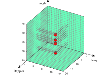
(a) Pilot at BS

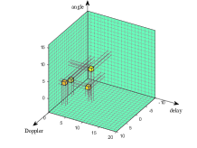
(b) 3D channel

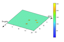
(c) Observation at user side

Figure 5: The channel dispersion over the delay-Doppler-angle domain.

Let us define the $M\!\!\times\!\!1$ vectors $\bar{\mathbf{h}}_{k,l,n}\!\!\!=\!\!\![\!\bar{h}_{k,l,n,\!-\!\frac{M}{2}}\!,\!\ldots\!,\!\bar{h}_{k,l,n,0}\!,\!\ldots\!,\!\bar{h}_{k,l,n,\frac{M}{2}\!-\!1}\!]^{T}$, $\mathbf{x}_{l,n}\!\!\!=\!\!\![\!x_{l,n,0},\!\ldots,\!x_{l,n,M\!-\!1}\!]^{T}$, $\bar{\mathbf{x}}_{l,n}=[\bar{x}_{l,n,0},\ldots,\bar{x}_{l,n,M-1}]^{T}=\mathbf{F}_{M}^{*}\mathbf{x}_{l,n}$, and $P\times 1$ vector $\mathbf{\bar{h}}^{no}_{k}=[\bar{h}_{k,i_{k,1},j_{k,1},q_{k,1}},\ldots,\bar{h}_{k,i_{k,P},j_{k,P},q_{k,P}}]^{T}$ for further use, where $l\in[0,L_{D}-1]$ and $n\in[0,N_{D}-1]$. Correspondingly, we give the $L_{D}\times N_{D}$ matrices $\mathbf{\bar{X}}_{s}$, whose $(l,n)$-th element is $[\bar{\mathbf{x}}_{l,n}]_{s}$ and $s\in[0,M-1]$. Moreover, the angle signature set for the user $k$ is given as $\mathcal{Q}_{k}^{a}=\!\{q_{k,p}\}_{p=1}^{P}$, and the maximum dispersion length along the delay and Doppler directions are separately written as

$$l^{G}=\max\{\{i_{k,p}\}_{p=1}^{P}\}_{k=1}^{K},\kern 10.0ptn^{G}=\max\{\{|j_{k,p}|\}_{p=1}^{P}\}_{k=1}^{K}.$$ (46)

Then, we can rewrite (3) as follows

$${y_{k,l,n}}{=} {\sum_{m=0}^{M-1}\sum_{p=1}^{P}e^{\jmath 2\pi\frac{(l-i_{k,p})j_{k,p}}{N_{D}(L_{D}+L_{cp})}}\tilde{h}_{k,i_{k,p},j_{k,p},m}x_{(l-i_{k,p})_{L_{D}},\langle n-N_{D}/2-j_{k,p}\rangle+N_{D}/2,m}+w_{k,l,n}}$$

$${=} {\sum_{p=1}^{P}\!e^{\jmath 2\pi\frac{(l-i_{k,p})j_{k,p}}{N_{D}(L_{D}+L_{cp})}}\left(\mathbf{F}^{H}_{M}\mathbf{\bar{h}}_{k,i_{k,p},j_{k,p}}\right)^{T}\left(\mathbf{F}_{M}^{T}\bar{\mathbf{x}}_{(l-i_{k,p})_{L_{D}},\langle n-N_{D}/2-j_{k,p}\rangle+N_{D}/2}\right)+w_{k,l,n}}$$

$${=} {\sum_{p=1}^{P}e^{\jmath 2\pi\frac{(l-i_{k,p})j_{k,p}}{N_{D}(L_{D}+L_{cp})}}\!{\bar{x}_{(l-i_{k,p})_{L_{D}},\langle n-N_{D}/2-j_{k,p}\rangle+N_{D}/2,q_{k,p}+M/2}}\bar{h}_{k,i_{k,p},j_{k,p},q_{k,p}}+w_{k,l,n}}.$$ (47)

According to the characteristics of 3D channels $\bar{h}_{k,i,j,q}$, we design three training schemes and optimize the pilot pattern over the 3D cubic space $\{(l,n,s)|l\in[0,L_{D}-1],n\in[0,N_{D}-1],s\in[0,M-1]\}$, which contains $M$ layers along the angle direction. Explicitly, the $s$-th layer is $\mathbf{\bar{X}}_{s}$.

IV-B1 The Case that All Paths of the User $k$ are Orthogonal over Delay-Doppler domain

Interestingly, we analyze one special case, where different scattering paths of the user $k$ have distinguished delays or Doppler frequencies. To fully exploit the energy dispersion effective of the OTFS, we adopt the embedded pilot structure [24] to estimate $\bar{h}_{k,i,j,q}$ and place only one effective pilot within fixed rectangle area of $\mathbf{\bar{X}}_{s}$. Without loss of generality, this training part is fixed in the region $\{(l,n)|l\in[0,\ldots,l^{G}],$ $n\in[0,\ldots,2n^{G}]\}$ of $\mathbf{\bar{X}}_{s}$. With the previous results, it can be checked that the user $k$ can receive signal from $P$ layers within the 3D cubic region, i.e., $\bar{\mathbf{X}}_{q_{k,p}+M/2}$, $p\!=\!1,2,\ldots,P$. Taking all the $K$ users into consideration, we would fix only one non-zero pilot at ${\bar{x}}_{0,n^{G},q+M/2}\!\!=\!\!\sqrt{{\sigma_{p}^{2}}}$, where $q\!\!\in\!\!\{\mathcal{Q}^{a}_{1}\!\cup\!\mathcal{Q}^{a}_{2}\!\cup\!\ldots\!\cup\!\mathcal{Q}^{a}_{K}\}$ and $\sigma_{p}^{2}$ is the training power.

With (47), it can be determined that the user $k$ achieves the non-zero training power at $P$ grids $\{y_{k,i_{k,1},n^{G}+j_{k,1}},y_{k,i_{k,2},n^{G}+j_{k,2}},\ldots,y_{k,i_{k,P},n^{G}+j_{k,P}}\}$, which separately correspond to the elements in $\mathbf{\bar{h}}^{no}_{k}$. Moreover, $y_{k,i_{k,p},n^{G}_{k}+j_{k,p}}$, $p\in[1,P]$, can be given as

$${y_{k,i_{k,p},n^{G}_{k}+j_{k,p}}=} {\bar{x}_{0,n_{k}^{G},q_{k,p}+M/2}}{\bar{h}_{k,i_{k,p},j_{k,p},q_{k,p}}+w_{k,i_{k,p},n^{G}_{k}+j_{k,p}},}$$

$${=} {\sqrt{{\sigma_{p}^{2}}}\bar{h}_{k,i_{k,p},j_{k,p},q_{k,p}}+w_{k,i_{k,p},n^{G}_{k}+j_{k,p}}.}$$ (48)

Then, we can obtain

$${\widehat{\bar{h}}_{k,i_{k,p},j_{k,p},q_{k,p}}=\sqrt{\frac{1}{\sigma_{p}^{2}}}y_{k,i_{k,p},n^{G}_{k}+j_{k,p}}.}$$ (49)

IV-B2 The Case that Different Paths of the User $k$ are Orthogonal over Angle Domain

We consider the case where different scattering paths of the user $k$ have distinguished angles, $k\!\!=\!\!1,2,\ldots,K$. For clear explanation, we firstly consider one user $k$. Without loss of generality, we assume that BS would send the user $k$ effective data from the rectangle region of the $P$ effective layers, i.e., $\bar{\mathbf{X}}_{q_{k,p}\!+\!\frac{M}{2}}$, $p\!\!=\!\!1,2,\ldots,P$. Specially, in $\bar{\mathbf{X}}_{q_{k,p}\!+\!\frac{M}{2}}$, the effective data lie in the region $\{(l,n)|l\!\!\in\!\![l_{k,p},l_{k,p}\!+\!W_{d}\!-\!1],n\!\!\in\!\![n_{k,p},n_{k,p}\!+\!W_{D}\!-\!1]\}$, where $W_{d}$ and $W_{D}$ are the maximum lengthes of this region along the delay and Doppler directions, respectively. Then, the user $k$ would receive $P$ signal components along different scattering paths, and each component has the same size with $\mathbf{Y}_{k}$. Here, we denote the $p$-th received signal part from $\bar{\mathbf{X}}_{q_{k,p}\!+\!\frac{M}{2}}$ as $\mathbf{Y}_{k,p}$, which experiences the channel $\bar{h}_{k,i_{k,p},j_{k,p},q_{k,p}}$. Correspondingly, $[\mathbf{Y}_{k,p}]_{l,n}$ can be derived from (47) as

$$[\mathbf{Y}_{k,p}]_{l,n}=e^{\jmath 2\pi\frac{(l-i_{k,p})j_{k,p}}{N_{D}(L_{D}+L_{cp})}}\bar{h}_{k,i_{k,p},j_{k,p},q_{k,p}}[\bar{\mathbf{X}}_{q_{k,p}+M/2}]_{(l-i_{k,p})_{L_{D}},\langle n-N_{D}/2-j_{k,p}\rangle+N_{D}/2},$$ (50)

which means that each grid in $\mathbf{Y}_{k,p}$ is associated only one symbol in $\mathbf{\overline{X}}_{q_{k,p}+M/2}$. Then, $\mathbf{Y}_{k}$ can be rewritten as

$$\mathbf{Y}_{k}=\sum_{p=1}^{P}\mathbf{Y}_{k,p}+\mathbf{W}_{k},$$ (51)

where the $(l,n)$-th element of $\mathbf{W}_{k}$ is equal to $w_{k,l,n}$.

To simply capture the path diversity, we align the associated grids for $[\mathbf{\bar{X}}_{q_{k,1}+M/2}]_{l_{k,1}+u,n_{k,1}+v}$, $[\mathbf{\bar{X}}_{q_{k,2}+M/2}]_{l_{k,2}+u,n_{k,2}+v}$$\ldots$ $[\mathbf{\bar{X}}_{q_{k,P}+M/2}]_{l_{k,P}+u,n_{k,P}+v}$ to the same position, $u\in[0,W_{d}-1],v\in[0,W_{D}-1]$. Hence, the related positions for $P$ effective data rectangles over the 3D cubic area should satisfy $(l_{k,1}+i_{k,1})_{L_{D}}=(l_{k,2}+i_{k,2})_{L_{D}}=\cdots=(l_{k,P}+i_{k,P})_{L_{D}}$ and $(n_{k,1}+j_{k,1})_{N_{D}}=(n_{k,2}+j_{k,2})_{N_{D}}=\cdots=(n_{k,P}+j_{k,P})_{N_{D}}$, which is shown in Fig. 6.

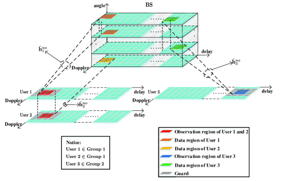
Figure 6: Path scheduling under the multi-user case.

Without loss of generality, we restrict the effective observation region of user $k$ in one rectangle of $\mathbf{Y}_{k}$, which can be described by the grid set $\mathcal{A}_{k}^{r}$ as

$${\mathcal{A}_{k}^{r}=\left\{(l,n)|l\in[l_{k},l_{k}+W_{d}-1],n\in[n_{k},n_{k}+W_{D}-1]\right\}},$$ (52)

where the element in $\mathcal{A}_{k}^{r}$ is the index of effective observation grid. Then, for $(l,n)\in\mathcal{A}_{k}^{r}$, it receives the information from $P$ grids within the 3D cubic area, whose specific locations in $\bar{\mathbf{X}}_{s}$ can be written as $\{((l-i_{k,1})_{L_{D}},\langle n-N_{D}/2-j_{k,1}\rangle+N_{D}/2,q_{k,1}+M/2),((l-i_{k,2})_{L_{D}},\langle n-N_{D}/2-j_{k,2}\rangle+N_{D}/2,q_{k,2}+M/2),\ldots,((l-i_{k,P})_{L_{D}},\langle n-N_{D}/2-j_{k,P}\rangle+N_{D}/2,q_{k,P}+M/2)\}$. Then, with respect to $\mathcal{A}_{k}^{r}$, the effective transmission region of the $\mathbf{\bar{X}}_{q_{k.p}+\frac{M}{2}}$ can be written as

$${\mathcal{A}^{t}_{k,p}=}\Big{\{} (l,n)|l=(l^{\prime}-i_{k,p})_{L_{D}},n=\langle n^{\prime}-N_{D}/2-j_{k,p}\rangle+N_{D}/2,(l^{\prime},n^{\prime})\in\mathcal{A}^{r}_{k}\Big{\}}.$$ (53)

Thus, combine (50) and (51), we obtain

$${[\mathbf{Y}_{k}]_{\mathcal{A}^{r}_{k}}}= \sum_{p=1}^{P}\underbrace{\bar{\boldsymbol{\Phi}}_{q_{k,p}+M/2}\odot[\bar{\mathbf{X}}_{q_{k,p}+M/2}]_{\mathcal{A}^{t}_{k,p}}}_{\bar{\mathbf{X}}^{e}_{k,q_{k,p}+M/2}}\bar{h}_{k,i_{k,p},j_{k,p},q_{k,p}}+[\mathbf{W}_{k}]_{\mathcal{A}^{r}_{k}}$$

$$= [\bar{\mathbf{X}}^{e}_{k,q_{k,1}+M/2},\ldots,\bar{\mathbf{X}}^{e}_{k,q_{k,P}+M/2}]\bar{\mathbf{h}}_{k}^{no}+[\mathbf{W}_{k}]_{\mathcal{A}^{r}_{k}},$$ (54)

where $[\bar{\boldsymbol{\Phi}}_{q_{k,p}\!+\!M/2}]_{u,v}\!=\!e^{\jmath 2\pi\frac{(l_{k}\!+\!u\!-\!i_{k,p})j_{k,p}}{N_{D}(L_{D}\!+\!L_{cp})}}$, $u\!\in\![0,W_{d}\!-\!1]$, $v\in[0,W_{D}\!-\!1]$ and the $W_{d}\!\times\!W_{D}$ matrix $\bar{\mathbf{X}}^{e}_{k,q_{k,p}+M/2}$ is given above.

Since only $P$ unknown channel gains should be estimated, we choose $P$ symbols in $\mathcal{A}_{k}^{r}$ as the training observation grids, whose indexes can be listed as $\{(l_{k},n_{k}),(l_{k},n_{k}+1),\ldots,(l_{k},n_{k}+P-1)\}$. Correspondingly, we have

$${[\mathbf{Y}_{k}]_{l_{k},n_{k}:n_{k}+P-1}}=\underbrace{\big{[}[\bar{\mathbf{X}}^{e}_{k,q_{k,1}+M/2}]_{0,0:P-1},\ldots,[\bar{\mathbf{X}}^{e}_{k,q_{k,P}+M/2}]_{0,0:P-1}\big{]}}_{\mathbf{T}_{k}}\bar{\mathbf{h}}_{k}^{no}+[\mathbf{W}_{k}]_{l_{k},n_{k}:n_{k}+P-1},$$ (55)

where the $P\times P$ training matrix $\mathbf{T}_{k}$ is defined in the above equation. Then, with LS estimator, we can obtain

$${\bar{\mathbf{h}}_{k}^{no}=\mathbf{T}_{k}^{-1}[\mathbf{Y}_{k}]_{l_{k},n_{k}:n_{k}+P-1},}$$ (56)

where the optimal training matrix should satisfy $\mathbf{T}_{k}^{H}\mathbf{T}_{k}=\sigma_{p}^{2}\mathbf{I}_{P}$.

The above strategy can be extended for the multi-user case. Due to the inter-user interference, it is necessary to schedule $\mathcal{A}^{t}_{k,p}$ to assure the effective transmitting regions for different users do not overlap in the 3D cubic area. To fully exploit the super resolution over the angle domain, we schedule the users with two steps: within the first step, the users would be separated over the angle domain, while in the second step, we further separate the users, that have overlapped angle signatures, in the delay-Doppler domain. Then, the users with non-overlapped angle signatures sets are allocated to the same group $\mathcal{G}_{g}$ $(g=1,2,\ldots,G)$, i.e.,

$${\mathcal{Q}_{k_{1}}^{a}\cap\mathcal{Q}_{k_{2}}^{a}=\emptyset,\kern 10.0pt\text{dist}(\mathcal{Q}_{k_{1}}^{a},\mathcal{Q}_{k_{2}}^{a})\geq D_{\theta},}$$ (57)

where $\text{dist}(\mathcal{Q}^{a}_{k_{1}}\!,\mathcal{Q}^{a}_{k_{2}})\!\!\triangleq\!\!\min\!|q_{k_{1},p}\!-\!q_{k_{2},p}|,\forall\!q_{k_{1},p}\!\in\!\mathcal{Q}^{a}_{k_{1}},\forall\!q_{k_{2},p}\!\in\!\mathcal{Q}^{a}_{k_{2}}$, and the protection gap $D_{\theta}$ is added to mitigate the effect of the channel power leakage along the angle direction. For $k_{1},k_{2}\in\mathcal{G}_{g}$, we assign them the same observation region over the delay-Doppler domain, i.e., $\mathcal{A}^{r}_{k_{1}}=\mathcal{A}^{r}_{k_{2}}=\mathcal{A}^{r}_{\mathcal{G}_{g}}$, but different angle grids, i.e., $\mathcal{Q}_{k_{1}}^{a}\cap\mathcal{Q}_{k_{2}}^{a}=\emptyset$, $k_{1}\neq k_{2}$.

With different user groups $\mathcal{G}_{g_{1}}$, $\mathcal{G}_{g_{2}}$, we assign distinguished delay-Doppler domain observation regions to satisfy the following constraints:

$${\mathcal{A}^{r}_{\mathcal{G}_{g_{1}}}\cap\mathcal{A}^{r}_{\mathcal{G}_{g_{2}}}=\emptyset,\kern 10.0pt\text{dist}(\mathcal{A}^{r}_{\mathcal{G}_{g_{1}}},\mathcal{A}^{r}_{\mathcal{G}_{g_{2}}})\succ\{D_{\tau},D_{\nu}\},}$$ (58)

where $\text{dist}(\mathcal{A}^{r}_{g_{1}},\mathcal{A}^{r}_{g_{2}})\succ\{D_{\tau},D_{\nu}\}$ means $\min|l_{1}\!-\!l_{2}|\!\geq\!D_{\tau}$ or $\min\!|n_{1}\!-\!n_{2}|\!\geq\!D_{\nu}$, $\forall(l_{1},n_{1})\!\in\!\mathcal{A}^{r}_{g_{1}},\forall(l_{2},n_{2})\!\in\!\mathcal{A}^{r}_{g_{2}}$, and the guard gaps $D_{\tau}$ and $D_{\nu}$ are mainly utilized to combat the dispersion effect of the 3D channels $\bar{h}_{k,i,j,q}$ along the delay and Doppler directions, respectively. Typically, we can separately set $D_{\tau}$ and $D_{\nu}$ as $D_{\tau}=l^{G}$ and $D_{\nu}=2n^{G}$. One typical example is presented in Fig. 7. After scheduling, the BS can map different users’ respective data with the scheduled delay-Doppler-angle domain grids, send the different data to the users within the same OTFS block, and occupy different 3D resources. Then, the users can parallel demap and decode respective data without inter-user interference.

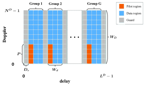
Figure 7: The observation regions for different users over the delay-Doppler domain.

IV-B3 General Case

Unfortunately, in practice, all paths of one user may be not distinguished over the angle or delay-Doppler domains. Theoretically, we can schedule the delay-Doppler-angle domain resources according to the overlapping situation of the paths and achieve effective channel estimation schemes, which is beyond the scope of this paper. Nonetheless, we present one feasible channel recovering method for this general case.

Taking all the $K$ users into consideration, we would fix the effective pilots of $\bar{\mathbf{X}}_{q\!+\!M/2}$ in the region $\{(l,n)|l\!\in\!(l_{s},l_{s}\!+\!H_{d}\!-\!1),n\!\in\!(n_{s}\!+\!H_{D}\!-\!1)\}$, where $q\!\in\!\{\mathcal{Q}^{a}_{1}\!\cup\!\mathcal{Q}^{a}_{2}\!\cup\!\ldots\!\cup\!\mathcal{Q}^{a}_{K}\}$, and $l_{s}$, $n_{s}$ separately denote the left and the bottom bounds of the effective pilot region within $\bar{\mathbf{X}}_{s}$. Moreover, $H_{d}$, $H_{D}$ are the maximum widths of the pilot region along the delay and Doppler axes, respectively. Moreover, we assume that the effective pilot region satisfies $l\!+\!i_{k,p}\!<\!L_{D}\!-\!1$ and $0\!<\!n\!+\!j_{k,p}\!<\!N_{D}\!-\!1$, where $\{{(l,n)}|l\!\!\in\!\!(l_{s},l_{s}\!+\!H_{d}\!-\!1),n\!\in\!(n_{s}\!+\!H_{D}\!-\!1)\}$, $k\!\in\![1,K]$, and $p\!\!\in\!\![1,P]$. Under this case, the observation regions for the pilots at all users are continuous regions.

With (47) and the delay-Doppler-angle signature for the user $k$, we can check that $y_{k,l,n}$ may have the non-zero entries within the region $\{(l,n)|l\in[l_{s}+i_{k}^{min},l_{s}+H_{d}-1+l^{G}],n\in[n_{s}+j_{k}^{min},n_{s}+H_{D}-1+j_{k}^{max}]\}$, where $i^{min}_{k}=\min~{}\{i_{k,p}\}_{p=1}^{P}$, $j_{k}^{min}=\min~{}\{j_{k,p}\}_{p=1}^{P}$, and $j_{k}^{max}=\max~{}\{j_{k,p}\}_{p=1}^{P}$. For simplicity, we rewrite (47) into the vector-matrix form. For user $k$, we can arrange $y_{k,l,n}$ within the region $\{(l,n)|l\in[l_{s}+i_{k}^{min},l_{s}+H_{d}-1+l^{G}],n\in[n_{s}+j_{k}^{min},n_{s}+H_{D}-1+j_{k}^{max}]\}$ into one column vector $\mathbf{y}^{e}_{k}\in\mathcal{C}^{(H_{d}+l^{G}-i_{k}^{min})(H_{D}+j_{k}^{max}-j_{k}^{min})\times 1}$, whose $\left((\!H_{D}\!+\!j_{k}^{max}\!-\!j_{k}^{min}\!)\!(\!l\!-\!(\!l_{s}\!+\!i_{k}^{min}\!)\!)\!+\!n\!-\!(\!n_{s}\!+\!j_{k}^{min}\!)\right)$-th elements equal to $y_{k,l,n}$. Finally, we can obtain the rewritten received signal (47) as

$${\mathbf{y}^{e}_{k}=\underbrace{\mathbf{V}^{e}_{k}\odot\bar{\mathbf{X}}^{e}_{k}}_{\boldsymbol{\Psi}^{e}_{k}}\mathbf{\bar{h}}^{no}_{k}+\mathbf{w}^{e}_{k},}$$ (59)

where the $\bar{\mathbf{X}}^{e}_{k}\in\mathcal{C}^{(H_{d}+l^{G}-i_{k}^{min})(H_{D}+j_{k}^{max}-j_{k}^{min})\times P}$ is the two-dimensional periodic convolution matrix with the $\left((H_{D}+j_{k}^{max}-j_{k}^{min})(l-(l_{s}+i_{k}^{min}))+n-(n_{s}+j_{k}^{min}),p-1\right)$-th element of $\bar{\mathbf{X}}^{e}_{k}$ being equal to $\bar{x}_{l-i_{k,p},n-j_{k,p},q_{k,p}}$, $\mathbf{V}^{e}_{k}\in\mathcal{C}^{(H_{d}+l^{G}-i_{k}^{min})(H_{D}+j_{k}^{max}-j_{k}^{min})\times P}$ is a matrix with the $\left((H_{D}+\!j_{k}^{max}-j_{k}^{min})(l-(l_{s}+i_{k}^{min}))+n-(n_{s}+j_{k}^{min}),p-1\right)$-th element being $e^{\jmath 2\pi\frac{(l-i_{k,p})j_{k,p}}{N_{D}(L_{D}+L_{cp})}}$, and $\mathbf{w}^{e}_{k}$ is the AWGN vector, whose element has zero mean and variance $\sigma^{2}$. Finally, by using LS method we can obtain

$${\hat{\bar{\mathbf{h}}}_{k}^{no}=\left((\boldsymbol{\Psi}^{e}_{k})^{T}\boldsymbol{\Psi}^{e}_{k}\right)^{-1}(\boldsymbol{\Psi}^{e}_{k})^{T}\mathbf{y}^{e}_{k},}$$ (60)

where the matrix $(\boldsymbol{\Psi}^{e}_{k})^{T}\boldsymbol{\Psi}^{e}_{k}$ is low-dimensional.

IV-C Pilot Overhead Analysis

In our proposed DL channel estimation scheme, the training overhead comes from two parts: the UL channel parameter extraction and the DL 3D channel recovering, where the former happens over the frequency-time-antenna domain while the latter lies in the delay-Doppler-angle domain. With respect to the first part, we utilize the time domain training sequence of length $K(L_{cp}+N_{t})$. Then, along the DL, we construct three training schemes over delay-Doppler-angle domain according to the characteristics of the scattering paths. When all paths of any user can be separated over the delay-Doppler domain, no more than $\min\{KP,M\}$ grids over the delay-Doppler-angle domain are needed. Moreover, if all paths of any user can be distinguished over the delay-Doppler domain, it takes us $KP^{2}$ grids in the 3D cubic resource region to estimate the gains for all DL scattering paths. With respect to the general case, the pilot overhead is $\min\{KPH_{d}H_{D},MH_{d}H_{D}\}$ at most, where $H_{d}$ and $H_{D}$ can be appropriately selected according to (60). It is noticed that the work in [26] only considers DL. However, in practice, the communication happens along both DL and UL. If [26] analyze the UL OTFS channel estimation, the similar pilot overhead with ours would be utilized. Moreover, the authors in [26] only focus the channel estimation but not the data transmission process for multiple users. In our work, we have given some feasible schemes for serving multiple users with the massive MIMO-OTFS. The proper path scheduling algorithm is given to avoid the inter-user interference.

V Simulation Results

In this section, we evaluate the performance of our algorithm through numerical simulation. Unless otherwise specified, we consider the TDD model. The number of BS’s antennas is $M=64$, the carrier frequency is $6$ GHz, and the antenna spacing $d$ is set as the half wavelength. The $K$ users move at the speed $v_{s}\in[200,400]$ Km/h, and their maximal Doppler shift frequency is $2.22$ kHz. With respect to the massive MIMO-OTFS scheme, the number of the subcarriers is $L_{D}=512$, the number of the OFDM symbols within one OTFS block is $N_{D}=128$, the length of CP is $L_{cp}=32$, and the sampling time period $T_{s}=\frac{1}{20\ \text{MHz}}$. Correspondingly, the resolutions over the delay and the Doppler domains are $T_{s}$ and $\frac{1}{(L_{D}+L_{cp})N_{D}T_{s}}\approx 287$ Hz, respectively. For the high mobility channel parameters, $\tau_{k,p}$ is randomly chosen from $\{0,T_{s},2T_{s},\ldots,15T_{s}\}$, while $\theta_{k,p}$ and $\nu_{k,p}$ are uniformly distributed within $[-10^{\circ},50^{\circ}]$ and $[-2.22,2.22]$ kHz, respectively. Moreover, the power of multi-path channel gain $h_{k,p}$ is normalized as 1, i.e., $\sum\limits_{p=1}^{P}\mathbb{E}\{|h_{k,p}|^{2}\}=1$. Furthermore, in our simulations, the angle grids $\vartheta_{n}$ lie uniformly within $[-90^{\circ},90^{\circ}]$, and the number of the angle grids is $90$. For the delay grids, the total number is $L=20$, and the delay girds can be written as $\{0,T_{s},\ldots,19T_{s}\}$.

The signal-to-noise ratio (SNR) is expressed as $\text{SNR}=10\log_{10}\sigma_{p}^{2}/\sigma^{2}$ dB. Here, we use the normalized mean square error (MSE) for both UL channel parameters $\mathbf{g}_{k}^{ul}$, $\boldsymbol{\beta}_{k}^{ul}$, $\boldsymbol{\upsilon}_{k}^{ul}$, $\bar{\mathbf{h}}^{no}_{k}$ and DL delay-Doppler-angle channel vector $\bar{\mathbf{h}}^{no}_{k}$ as the performance metric, which is defined as

$$\text{MSE}_{\mathbf{x}}=\mathbb{E}\left\{\frac{||\hat{\mathbf{x}}-\mathbf{x}||^{2}}{||\mathbf{x}||^{2}}\right\},\mathbf{x}=\mathbf{g}_{k}^{ul},\boldsymbol{\beta}_{k}^{ul},\boldsymbol{\upsilon}_{k}^{ul},\bar{\mathbf{h}}^{no}_{k},$$ (61)

where $\hat{\mathbf{x}}$ is the estimation of $\mathbf{x}$.

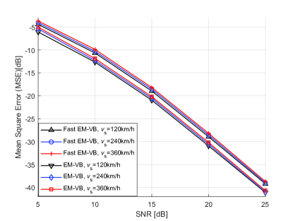
Figure 8: The MSEs of $\mathbf{g}_{k}^{ul}$ versus SNRs at different users’ moving speeds.

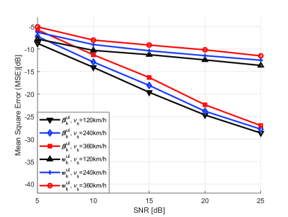
Figure 9: The MSEs of $\boldsymbol{\beta}_{k}^{ul}\!,\!\boldsymbol{\upsilon}_{k}^{ul}$ versus SNRs at different users’ moving speeds.

Fig. 8 and Fig. 9 shows the MSE performance for $\mathbf{g}_{k}^{ul}$ and $\boldsymbol{\beta}_{k}^{ul}$, $\boldsymbol{\upsilon}_{k}^{ul}$ at different SNRs, where three mobility conditions, i.e., $v_{s}=120,240,360$ Km/h, are considered. Moreover, we set the number of paths and observation points as $P=12$ and $N_{t}=40$, respectively. Notice that we use the notation “fast EM-VB” to denote the low complex EM-VB algorithm. As shown in Fig. 8 and Fig. 9, the MSE decreases as the SNR increases. Besides, the bigger the speed $v_{s}$ is, the higher the MSE curves of $\mathbf{g}_{k}^{ul}$, $\boldsymbol{\beta}_{k}^{ul}$, and $\boldsymbol{\upsilon}_{k}^{ul}$ are. However, the difference is very little, which is not the same with the case in [19]. This is because that we directly recover the physical intrinsic parameters $\{\tau_{k,l}^{ul},\upsilon_{k,l}^{ul},\theta_{k,l}^{ul}\}$ but not the mobility channels. Furthermore, it can be seen from Fig. 8 that the performance of our proposed fast EM-VB is only $2\sim 3$ dB lower than that of EM-VB, which shows the effectiveness and robustness of fast EM-VB. Notice that, in Fig. 9, we only present the fast EM-VB performance for the clarity. In the following, all our present performance curves are from the fast EM-VB.

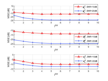
Figure 10: The MSE curves of the channel parameters versus $l^{EM}$.

In Fig. 10, we give the MSE curves of the channel parameters versus the EM iteration index $l^{EM}$. Two different SNRs, i.e., 10dB and 20dB, are examined. Same with Fig. 8, we set $P=12$, and $N_{t}=40$. It can be checked from Fig.10 only five iterations are needed for $\boldsymbol{\beta}_{k}^{ul},\boldsymbol{\upsilon}_{k}^{ul}$, and $\mathbf{g}_{k}^{ul}$ to achieve their steady states.

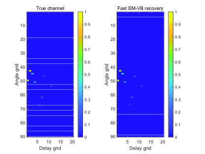
Figure 11: The true and recovered locations of the non-zero elements for $\tilde{\mathbf{G}}_{k}^{ul}$.

Fig. 11 displays the true and estimated locations of the nonzero elements within $\tilde{\mathbf{G}}_{k}^{ul}$. It can be found that there are only $P=12$ dominant paths for user $k$. Moreover, from the two sub-figures, we can find the accurate support recovery capability of our algorithm.

In Fig. 12, we study the MSE performance of $\mathbf{g}^{ul}_{k}$’s estimation with respect to the number of observations $N_{t}$, where $P=12$, and $\text{SNR}=5,10,15,20,25$ dB. It can be found that with the number of observations increasing, the MSEs for all SNRs gradually decrease and would converge to different steady states. Moreover, the higher the SNR is, the faster the MSE curves would converge. The above observations are not unexpected and can be explained as follows. Much more observations can help us determine the nonzero locations of $\mathbf{g}^{ul}_{k}$ in one easier way, which could enhance the estimation performance of $\mathbf{g}^{ul}_{k}$. However, the MSEs of $\mathbf{g}^{ul}_{k}$ are determined by the training power and the noise variance. With different $P$ at fixed SNR, the training power is fixed. Hence, increasing of $P$ can make sure that MSEs of $\mathbf{g}^{ul}_{k}$ always decrease.

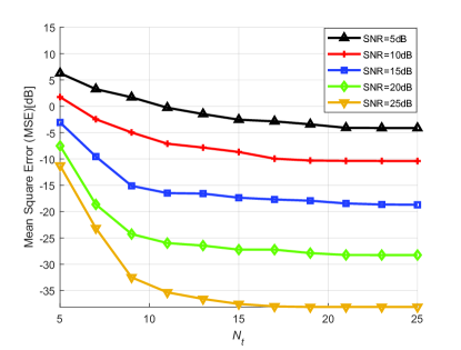
Figure 12: The MSE performance of $\mathbf{g}^{ul}_{k}$’s estimation with respect to $N_{t}$.

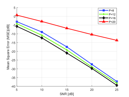
Figure 13: The MSEs of $\mathbf{g}_{k}^{ul}$ under different sparsity conditions.

In order to examine the impact of $\mathbf{g}_{k}^{ul}$’s sparsity on its estimation performance, we present $\mathbf{g}_{k}^{ul}$’s MSE curves with different $P$ in Fig. 13. Moreover, $N_{t}$ is fixed as 18, which means that the maximum unknown parameters that low complex VB-EM can effectively estimate is $18$. Hence, the bigger $P$ is, the less sparse $\mathbf{g}_{k}^{ul}$ will be. From Fig. 13, we have the following observations: If $P$ is smaller than $N_{t}$, the MSE curves of $\mathbf{g}_{k}^{ul}$ decrease with the increasing of $P$, which is because that it is difficult for the low complex EM-VB to determine the few nonzero locations of $\mathbf{g}_{k}^{ul}$. However, when $P$ becomes bigger than $N_{t}$, we can not construct enough independent observation equations for unknown nonzero elements in $\mathbf{g}_{k}^{ul}$, even if the exact nonzero locations of $\mathbf{g}_{k}^{ul}$ are known.

Finally, we show the MSE curves for the DL delay-Doppler-angle domain $\bar{h}_{k,i,j,q}$. Here, the case that different paths of the user $k$ are orthogonal over angle domain is considered. The FDD model is considered here, where the carrier frequency along the DL is set as $5.98$ GHz. Moreover, the corresponding performance for the methods in [19] are also presented for comparison. In order to apply the scheme in [19], we adopt the CE-BEM to describe the time-varying massive MIMO channels with BEM coefficient vectors over the time domain, and utilize the framework in [19] to track different BEM coefficient vectors in different OFDM symbols. Then, we construct the high mobility channel in the time domain, and use (4), (5) to obtain the corresponding delay-Doppler-angle domain channel. From Fig. 14, we can see that the performance of the massive MIMO-OTFS based DL channel estimator is much better than that of block fading based method. Moreover, similar to Fig. 8 and Fig. 14, different form the block fading based method, the performance of the massive MIMO-OTFS based DL channel estimator is not closely coupled with the users’ mobility speeds.

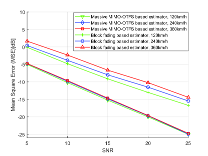
Figure 14: The MSEs of $\bar{\mathbf{h}}^{no}_{k}$ under different sparsity conditions.

VI Conclusion

In this paper, we examined the UL-aided high mobility DL channel estimation scheme for the massive MIMO-OTFS networks. The EM-VB framework was utilized to recover the UL channel parameters including the angles, the delays, the Doppler frequencies, and the channel gains. Then, we resorted to the fast Bayesian inference to design one low complex EM-VB. Correspondingly, the angle, the delay, and the Doppler reciprocity between UL and DL was fully exploited to reconstruct the parameters for DL channels at BS. Furthermore, DL massive MIMO channel estimation over the delay-Doppler-angle domain was carefully studied. Within this phase, we analyzed the channel dispersion of the OTFS over the delay-Doppler domain and designed three DL 3D channel training schemes according to the scattering characteristics over the 3D angle-delay-Doppler domain. Simulation results showed that our proposed strategy is valid and has strong robustness.

References

- [1] J. Zhang, S. Chen, Y. Lin, J. Zheng, B. Ai and L. Hanzo, “Cell-free massive MIMO: A new next-generation paradigm,” IEEE Access., vol. 7, pp. 99878-99888, 2019.
- [2] F. Rusek, D. Persson, B. K. Lau, E. G. Larsson, T. L. Marzetta, O. Edfors, and F. Tufvesson, “Scaling up MIMO: Opportunities and challenges with very large arrays,” IEEE Signal Process. Mag., vol. 30, no. 1, pp. 40-60, Jan. 2013.
- [3] V. Jungnickel, K. Manolakis, W. Zirwas, B. Panzner, V. Braun, M. Lossow, M. Sternad, R. Apelfrojd, and T. Svensson, “The role of small cells, coordinated multipoint, and massive MIMO in 5G,” IEEE Commun. Mag., vol. 52, no. 5, pp. 44-51, May. 2014.
- [4] J. Zhang, L. Dai, X. Li, Y. Liu and L. Hanzo, “On low-resolution ADCs in practical 5G millimeter-wave massive MIMO systems,” IEEE Commun. Mag., vol. 56, no. 7, pp. 205-211, July. 2018.
- [5] C. D. Ho, H. Q. Ngo, M. Matthaiou and T. Q. Duong, “On the performance of zero-forcing processing in multi-way massive MIMO relay networks,” IEEE Commun. Lett., vol. 21, no. 4, pp. 849-852, April. 2017.
- [6] W. Tan, M. Matthaiou, S. Jin, and X. Li, “Spectral efficiency of DFT-based processing hybrid architectures in massive MIMO” IEEE Wireless Commun. Lett., vol. 6, no. 5, pp. 586-589, Oct. 2017.
- [7] A. Adhikary, J. Nam, J. Y. Ahn, and G. Caire, “Joint spatial division and multiplexing the large-scale array regime,” IEEE Trans. Inf. Theory, vol. 59, no. 10, pp. 6441-6463, Oct. 2013.
- [8] J. Nam, A. Adhikary, J. Y. Ahn, and G. Caire, “Joint spatial division and multiplexing: Opportunistic beamforming, user grouping and simplified downlink scheduling,” IEEE J. Sel. Topics Signal Process., vol. 8, no. 5, pp. 876-890, Oct. 2014.
- [9] J. Zhang, X. Xue, E. Bjornson, B. Ai and S. Jin, “Spectral efficiency of multipair massive MIMO two-way relaying with hardware impairments,” IEEE Wireless Commun. Lett., vol. 7, no. 1, pp. 14-17, Feb. 2018.
- [10] A. Adhikary, E. A. Safadi, M. K. Samimi, R. Wang, G. Caire, T. S. Rappaport, and A. F. Molisch, “Joint spatial division and multiplexing for mm-Wave channels,” IEEE J. Sel. Areas Commun., vol. 32, no. 6, pp. 1239-1255, Jun. 2014.
- [11] H. Xie, F. Gao, S. Jin, J. Fang and Y. Liang, “Channel estimation for TDD/FDD massive MIMO systems with channel covariance computing,” IEEE Trans. Wireless Commun., vol. 17, no. 6, pp. 4206-4218, June. 2018.
- [12] Y. Han, T. Hsu, C. Wen, K. Wong and S. Jin, “Efficient downlink channel reconstruction for FDD multi-antenna systems,” IEEE Trans. Wireless Commun., vol. 18, no. 6, pp. 3161-3176, June. 2019.
- [13] A. Liao, Z. Gao, H. Wang, S. Chen, M. Alouini and H. Yin, “Closed-loop sparse channel estimation for wideband millimeter-wave full-dimensional MIMO systems,” IEEE Trans. Commun., vol. 67, no. 12, pp. 8329-8345, Dec. 2019.
- [14] M. Matthaiou, P. de Kerret, G. K. Karagiannidis and J. A. Nossek, “Mutual information statistics and beamforming performance analysis of optimized LoS MIMO systems,” IEEE Trans. Commun., vol. 58, no. 11, pp. 3316-3329, November. 2010.
- [15] H. Xie, F. Gao, S. Zhang, and S. Jin, “A unified transmission strategy for TDD/FDD massive MIMO systems with spatial basis expansion model,” IEEE Trans. Veh. Technol., vol. 66, no. 4, pp. 3170-3184, Apr. 2017.
- [16] Q. Qin, L. Gui, B. Gong and S. Luo, “Sparse channel estimation for massive MIMO-OFDM systems over time-varying channels,” IEEE Access, vol. 6, pp. 33740-33751, 2018.
- [17] J. Zhao, H. Xie, F. Gao, W. Jia, S. Jin and H. Lin, “Time varying channel tracking with spatial and temporal BEM for massive MIMO systems,” IEEE Trans. Wireless Commun., vol. 17, no. 8, pp. 5653-5666, Aug. 2018.
- [18] W. Guo, W. Zhang, P. Mu, F. Gao and H. Lin, “High-mobility wideband massive MIMO communications: Doppler compensation, analysis and scaling laws,” IEEE Trans. Wireless Commun., vol. 18, no. 6, pp. 3177-3191, Jun. 2019.
- [19] J. Ma, S. Zhang, H. Li, F. Gao and S. Jin, “Sparse Bayesian learning for the time-varying massive MIMO channels: Acquisition and tracking,” IEEE Trans. Commun., vol. 67, no. 3, pp. 1925-1938, Mar. 2019.
- [20] M. Li, S. Zhang, N. Zhao, W. Zhang, and X. Wang, “Time-varying massive MIMO channel estimation: Capturing, reconstruction and restoration,” IEEE Trans. Commun., vol. 67, no. 11, pp. 7558-7572, Nov. 2019.
- [21] R. Hadani, S. Rakib, S. Kons, M. Tsatsanis, A. Monk, C. Ibars, J. Delfeld, Y. Hebron, A. J. Goldsmith, A. F. Molisch and R. Calderbank, “Orthogonal time frequency space modulation,” arXiv:1808.00519, 2018. [Online]. Available: https://arxiv.org/abs/1808.00519.
- [22] R. Hadani, S. Rakib, A. F. Molisch, C. Ibars, A. Monk, M. Tsatsanis, J. Delfeld, A. Goldsmith, and R. Calderbank, “Orthogonal time frequency space (OTFS) modulation for millimeter-wave communications systems,” in Proc. IEEE International Microwave Symposium (IEEE IMS’17), Jun. 2017, pp. 681-683.
- [23] K. Murali, A. Chockalingam, “On OTFS modulation for high-Doppler fading channels,”arXiv:1802.00929, 2018. [Online]. Available: https://arxiv.org/abs/1802.00929.
- [24] P. Raviteja, K. T. Phan, and Y. Hong, “Embedded pilot-aided channel estimation for OTFS in delay-Doppler channels,” IEEE Trans. Veh. Technol., vol. 68, no. 5, pp. 4906-4917, May. 2019.
- [25] P. Raviteja, K. T. Phan, Y. Hong, and E. Viterbo, “Interference cancellation and iterative detection for orthogonal time frequency space modulation,” IEEE Trans. Wireless. Commun., vol. 17, no. 10, pp. 6501-6515, Oct. 2018.
- [26] W. Shen, L. Dai, J. An, P. Fan and R. W. Heath, “Channel estimation for orthogonal time frequency space (OTFS) massive MIMO,” IEEE Trans. Signal Process., vol. 67, no. 16, pp. 4204-4217, Aug. 2019.
- [27] J. Ma, S. Zhang, H. Li, N. Zhao and V. C. M. Leung, “Interference alignment and soft-space-reuse based cooperative transmission for multi-cell massive MIMO networks,” IEEE Trans. Wireless Commun., vol. 17, no. 3, pp. 1907-1922, Mar. 2018.
- [28] D. J. C. MacKay, “Bayesian interpolation,” Neural Comput., vol. 4, no. 3, pp. 415-447, May. 1992.
- [29] S. Ji, Y. Xue, and L. Carin, “Bayesian compressive sensing,” IEEE Trans. Signal Process., vol. 56, no. 6, pp. 2346-2356, Jun. 2008.
- [30] M. E. Tipping, “Sparse Bayesian learning and the relevance vector machine,” J. Mach. Learn. Res., vol. 1, pp. 211-244, Sep. 2001.
- [31] J. G. Serra, M. Testa, R. Molina and A. K. Katsaggelos, “Bayesian K-SVD using fast variational inference,” in IEEE Trans. Signal Process., vol. 26, no. 7, pp. 3344-3359, Nov. 2017.
- [32] M. J. Beal, Variational Algorithms for Approximate Bayesian Inference. London, U.K.: Univ. London, 2003.
- [33] J. Winn and C. M. Bishop, “Variational message passing,” J. Mach. Learn. Res., vol. 6, pp. 661-694, Apr. 2005.
- [34] M. Tipping and A. Faul, “Fast marginal likelihood maximisation for sparse Bayesian models,” in Proc. 9th Int. Workshop Artificial Intelligence and Statistics, C. M. Bishop and B. J. Frey, Eds., 2003.