Solving Non-Markovian Stochastic Control Problems driven by Wiener Functionals

Abstract.

In this article, we present a general methodology for stochastic control problems driven by the Brownian motion filtration including non-Markovian and non-semimartingale state processes controlled by mutually singular measures. The main result of this paper is the development of a numerical scheme for computing near-optimal controls associated with controlled Wiener functionals via a finite-dimensional approximation procedure. The theory does not require functional differentiability assumptions on the value process and ellipticity conditions on the diffusion components. Explicit rates of convergence are provided under rather weak conditions for distinct types of non-Markovian and non-semimartingale states. The analysis is carried out on suitable finite dimensional spaces and it is based on the weak differential structure introduced by [40, 41] jointly with measurable selection arguments. The theory is applied to stochastic control problems based on path-dependent SDEs and rough stochastic volatility models, where both drift and possibly degenerated diffusion components are controlled. Optimal control of drifts for nonlinear path-dependent SDEs driven by fractional Brownian motion with exponent $H\in(0,1)$ is also discussed. Finally, we present a simple numerical example to illustrate the method.

1. Introduction

Let $\mathbf{C}_{n,T}$ be the set of continuous functions from $[0,T]$ to $\mathbb{R}^{n}$, let $\xi:\mathbf{C}_{n,T}\rightarrow\mathbb{R}$ be a Borel functional, let $\mathbb{F}=(\mathcal{F}_{t})_{t\geq 0}$ be a fixed filtration and let $U^{T}_{t};0\leq t\leq T$ be a family of admissible $\mathbb{F}$-adapted controls defined over $(t,T]$. The goal of this paper is to develop a numerical scheme to solve a generic stochastic optimal control problem of the form

(1.1) $$\sup_{\phi\in U^{T}_{0}}\mathbb{E}\big{[}\xi\big{(}X^{\phi}\big{)}\big{]},$$

where $\{X^{\phi};\phi\in U^{T}_{0}\}$ is a given family of $\mathbb{F}$-adapted controlled continuous processes. A common approach to such generic control problem (see e.g [14, 20]) is to consider for each control $u\in U_{0}^{T}$, the value process given by

(1.2) $$V(t,u)=\operatorname*{ess\,sup}_{\phi;\phi=u~{}\text{on}~{}[0,t]}\mathbb{E}\big{[}\xi\big{(}X^{\phi}\big{)}|\mathcal{F}_{t}\big{]};0\leq t\leq T.$$

Two fundamental questions in stochastic control theory rely on sound characterizations of value processes and the development of concrete methods to produce either exact optimal controls $u^{*}\in U^{T}_{0}$ (when exists)

$$\mathbb{E}\big{[}\xi(X^{u^{*}})\big{]}=\sup_{\phi\in U^{T}_{0}}\mathbb{E}\big{[}\xi\big{(}X^{\phi}\big{)}\big{]},$$

or near-optimal controls (see e.g [57]) which realize

(1.3) $$\mathbb{E}\big{[}\xi(X^{u^{*}})\big{]}>\sup_{\phi\in U^{T}_{0}}\mathbb{E}\big{[}\xi\big{(}X^{\phi}\big{)}\big{]}-\epsilon,$$

for an arbitrary error bound $\epsilon>0$. Exact optimal controls may fail to exist due to e.g lack of convexity, moreover they are very sensitive to perturbations and numerical rounding. In this context, the standard approach is to consider near-optimal controls which exist under minimal hypotheses and are sufficient in most applications.

Two major tools for studying stochastic controlled systems are Pontryagin’s maximum principle and Bellman’s dynamic programming. While these two methods are known to be very efficient for establishing some key properties (e.g existence of optimal controls, smoothness of the value functional, sufficiency of subclasses of controls, etc), the problem of solving explicitly or numerically a given stochastic control problem remains a critical issue in the field of control theory. Indeed, except for a very few specific cases, the determination of an optimal control (either exact or near) is a highly nontrivial problem to tackle. The present article presents a systematic method to compute and characterize $u^{*}$ realizing (1.3) for a given stochastic control problem (1.2) driven by a generic controlled process.

In the Markovian case, a classical approach in solving stochastic control problems is given by the dynamic programming principle based on Hamilton-Jacobi-Bellman (HJB) equations. One popular approach is to employ verification arguments to check if a given solution of the HJB equation coincides with the value function at hand, and obtain as a byproduct the optimal control. Discretization methods also play an important role towards the resolution of the control problem. In this direction, several techniques based on Markov chain discretization schemes [37], Krylov’s regularization and shaking coefficient techniques (see e.g [35, 36]) and Barles-Souganidis-type monotone schemes [2] have been successfully implemented. We also refer the more recent probabilistic techniques on fully non-linear PDEs given by Fahim, Touzi and Warin [21] and the randomization approach of Kharroubi, Langrené and Pham [32, 33, 34].

Beyond the Markovian context, the value process (1.2) cannot be reduced to a deterministic PDE and the control problem (1.1) is much more delicate. Nutz [45] employs techniques from quasi-sure analysis to characterize one version of the value process as the solution of a second order backward stochastic differential equation (2BSDE) (see [53]) under a non-degeneracy condition on the diffusion component of a controlled non-Markovian stochastic differential equation driven by Brownian motion (henceforth abbreviated by CNM-SDE-BM). Nutz and Van Handel [44] derive a dynamic programming principle in the context of model uncertainty and nonlinear expectations. Inspired by the work [32], under the weak formulation of the control problem, Fuhrman and Pham [23] show a value process can be reformulated under a family of dominated measures on an enlarged filtered probability space where the CNM-SDE-BM might be degenerated. It is worth to mention that under a nondegeneracy condition on diffusion components of CNM-SDEs-BM, (1.2) can also be viewed as a fully nonlinear path-dependent PDE in the sense of [19] via its relation with 2BSDEs (see section 4.3 in [19]). In this direction, Possamaï, Tan and Zhou [48] derived a dynamic programming principle for a stochastic control problem w.r.t a class of nonlinear kernels. They obtained a well-posedness result for general 2BSDEs and established a link with path-dependent PDEs in possibly degenerated cases. We also drive attention to Qiu [50] who characterizes (1.2) driven by a CNM-SDE-BM as a solution of a suitable HJB-type equation and uniqueness is established under a non-degeneracy condition on the diffusion components. Under strong a priori functional differentiability conditions (in the sense of [18, 12]) imposed on (1.2), one can apply functional Itô’s formula to arrive at verification-type theorems. In this direction, we refer to e.g. Cont [13] and Saporito [52].

Discrete-type schemes for the optimal value (1.1) driven by CNM-SDEs-BM were studied in the context of G-expectations by Dolinsky [16] and also by Zhang and Zhuo [55], Ren and Tan [51] and Tan [54]. In [55, 51], the authors provide monotone schemes in the spirit of Barles-Souganidis for fully nonlinear path-dependent PDEs in the sense of [19] and hence one may apply their results for the study of (1.1). Under elipticity conditions, by employing weak convergence methods in the spirit of Kushner and Depuis, [54] provides a discretization method for the optimal value (1.1). Convergence rates are available only under strong regularity conditions on the value process (1.2) (see [55]) or in the state independent case [16, 54].

1.1. Main setup and contributions

The main contribution of this paper is the development of a new numerical scheme for computing near optimal controls of stochastic systems adapted to the Brownian motion filtration and parameterized by possibly mutually singular measures. In particular, we present a discrete-type approximation for a large class of nonlinear expectations driven by possibly non-Markovian and / or non-semimartingale controlled states. More importantly, our approximation is equipped with a suitable dynamic programming equation which allows us to compute near optimal controls much beyond the class of linear-quadratic optimal control problems. For instance, nonlinear controlled path-dependent degenerated SDEs driven by a possibly non-smooth Gaussian transformation of the Brownian motion is a typical application of our methodology. Under a rather weak $L^{2}$-type regularity condition imposed on controlled states, this article develops a concrete methodology to solve numerically a given stochastic control problem of the form (1.1). None differentiability condition on the value process (1.2) is required. Moreover, the scheme is implementable using e.g regression Monte-Carlo techniques

The methodology is based on a weak version of functional Itô calculus developed by Leão, Ohashi and Simas [41] and inspired by Leão and Ohashi [40]. A given Brownian motion structure is discretized which gives rise to differential operators acting on piecewise constant processes adapted to a jumping filtration in the sense of [31] and generated by what we call a discrete-type skeleton $\mathscr{D}=\{\mathcal{T},A^{k,j};j=1,\ldots,d,;k\geq 1\}$ (see Definition 3.1). For a given controlled state process $\{X^{\phi};\phi\in U_{0}^{T}\}$, we construct a controlled imbedded discrete structure $\big{(}(V^{k})_{k\geq 0},\mathscr{D}\big{)}$ (see Definition 3.2 in Section 3) for the value process (1.2). This is a non-linear version of the imbedded discrete structures introduced by [41] and it can be interpreted as a discrete version of (1.2).

By using measurable selection arguments, we aggregate the controlled imbedded discrete structure $\big{(}(V^{k})_{k\geq 0},\mathscr{D}\big{)}$ into a single finite sequence of upper semianalytic value functions $\mathbb{V}^{k}_{n}:\mathbb{H}^{k,n}\rightarrow\mathbb{R};n=0,\ldots,e(k,T)-1$. Here, $\mathbb{H}^{k,n}$ is the $n$-fold cartesian product of $\mathbb{A}\times\mathbb{S}_{k}$, where $\mathbb{A}$ is the action space, $\mathbb{S}_{k}$ is suitable finite-dimensional space which accommodates the dynamics of the structure $\mathscr{D}$ and $e(k,T)$ is a suitable number of steps to recover (1.1) over the entire period $[0,T]$ as the discretization level $k$ goes to infinity. This procedure allows us to derive a dynamic programming equation over $e(k,T)$ steps which is the building block to solve stochastic control problems much beyond the classical Markovian states, traditionally treated by Markov chain approximations and PDE methods. The dynamic programming principle presented in Section 5.1 allows us to select near optimal controls for (1.3) solely based on the discrete skeleton $\mathscr{D}$. We refer the reader to Section 7 for a simple numerical example which illustrates how one can make use of our methodology in a simple stochastic control problem.

The connection between the dynamic programming principle based on $\mathscr{D}$ and the original control problem (1.1) is made via a strong robustness property found in a wide class of Wiener functionals as described by [41] in the linear expectation case. In this work, we take one step ahead towards the fully non-linear case. A first elementary consequence of our discretization scheme (see Proposition 4.2) is the fact that an arbitrary nonlinear expectation (see e.g [47]) driven by a strongly controlled Wiener functional $(X,\mathcal{X})$ associated with a controlled imbedded discrete structure $\mathcal{X}=\big{(}(X^{k})_{k\geq 1},\mathscr{D}\big{)}$ (see Definition 3.3 in Section 3) is represented by

$$\sup_{\phi\in U^{T}_{0}}\mathbb{E}\big{[}\xi(X^{\phi})\big{]}=\lim_{k\rightarrow+\infty}\sup_{\phi\in U^{k,e(k,T)}_{0}}\mathbb{E}\big{[}\xi(X^{k,\phi})\big{]},$$

over a suitable set $U^{k,e(k,T)}_{0}$ of stepwise constant $\mathscr{D}$-adapted processes. The concept of strongly controlled Wiener functional covers a wide class of stochastic systems which cannot be reduced to Markovian states without adding infinitely many degrees of freedom (see Sections 1.2 and 6).

The main results of this article, Theorems 5.1 and 5.2, state that for the class of strongly controlled Wiener functionals, we construct a dynamic programming algorithm for the discrete time analog of the nonlinear expectation (1.1) and for the corresponding (near) optimal control $\phi^{\star,k,\epsilon}$ based on the skeleton $\mathscr{D}$. Furthermore, for a given error bound $\epsilon\geq 0$, the rate of convergence of our numerical scheme is proportional to

(1.4) $$\Big{|}\sup_{u\in U^{T}_{0}}\mathbb{E}\big{[}\xi\big{(}X^{u}\big{)}\big{]}-\mathbb{E}\big{[}\xi\big{(}X^{\phi^{*,k,\epsilon}}\big{)}\big{]}\Big{|}=O\Big{(}h_{k}+r_{k}+\epsilon\Big{)}$$

and

(1.5) $$\Bigg{|}\sup_{\phi\in U^{k,e(k,T)}_{0}}\mathbb{E}\big{[}\xi(X^{k,\phi})\big{]}-\sup_{\phi\in U^{T}_{0}}\mathbb{E}\big{[}\xi(X^{\phi})\big{]}\Bigg{|}=O(h_{k}+r_{k}),$$

as $k\rightarrow+\infty$. The rate $(h_{k})_{k\geq 1}$ in (1.4) and (1.5) depends on the degree of continuity of $X$ w.r.t a structure $\big{(}(X^{k})_{k\geq 1},\mathscr{D}\big{)}$ (see (3.10)) combined with large deviation principles related to a family of hitting times $(T^{k}_{n})_{n\geq 1}$. The rate $(r_{k})$ in (1.4) and (1.5) depends on an equiconvergence property (Theorem 11.1) for Brownian martingales w.r.t the structure $\mathscr{D}$ and it is independent of the controlled state.

In contrast to previous works, we remark that our approach does not rely on a given representation of the value process (1.2) in terms of path-dependent PDE or 2BSDE. We develop a fully pathwise structure $\mathbb{V}^{k}_{j};j=0,\ldots,e(k,T)-1$ which allows us to make use the classical theory of analytic sets to construct near-optimal controls appearing in (1.4) by means of a list of analytically measurable functions $C^{\epsilon}_{k,j}:\mathbb{H}^{k,j}\rightarrow\mathbb{A};j=0,\ldots,e(k,T)-1$ which can be calculated from (5.9) or (5.12) for a given error bound $\epsilon\geq 0$. By composing those functions with the skeleton $\mathscr{D}$, we are able to compute near optimal controls $\phi^{\star,k,\epsilon}$ realizing (1.4). More importantly, the whole dynamics on $\mathscr{D}$ can be simulated by means of the first time Brownian motion hits $\pm 1$ and Bernoulli random variables. The regularity conditions of the theory boils down to a mild $L^{2}$-type continuity hypothesis on the controlled state (see Assumption (B1)) combined with a Hölder modulus of continuity on the payoff functional $\xi$ (see Assumption (A1)).

In contrast to the framework of one fixed probability measure in [41], in the present context it is essential to aggregrate a given structure into a single deterministic finite sequence of maps due to a possible appearance of mutually singular measures induced by $X^{k,\phi}$ as $\phi$ varies over the set of controls $U^{k,e(k,T)}_{0}$. Moreover, we mention it is possible to prove a differential-type representation result for (1.2) by extending the framework of [41] to controlling probabilities via measurable selection arguments combined with Theorem 11.1. Since it is not our purpose to focus on the representation of (1.2), we leave this construction to a future work.

1.2. Examples

As a test of the relevance of the theory, we show that our methodology can be applied to controlled Wiener functionals of the form

$$X^{u}=F\big{(}B,(\alpha,\sigma)(X^{u},u)\big{)},$$

where the non-anticipative functionals $(\alpha,\sigma)$ admit Lipschitz regularity w.r.t. control variables which in turn implies $L^{2}$-Lipschitz regularity of $u\mapsto X^{u}$ w.r.t control processes (Assumption (B1)). We investigate three typical examples illustrating distinct types of path-dependency which fit into the theory developed in this paper:

(1.6) $$dX^{u}(t)=\alpha(t,X^{u},u(t))dt+\sigma(t,X^{u},u(t))dB(t),$$

(1.7) $$dX^{u}(t)=\alpha(t,X^{u},u(t))dt+\sigma dB_{H}(t),$$

and

(1.8) $$\left\{\begin{array}[]{lc}dX^{u}(t)=X^{u}(t)\mu(u(t))dt+X^{u}(t)\vartheta(Z(t),u(t))dB(t)\\ dZ(t)=\nu dB_{H}(t)-\beta(Z(t)-m)dt,\end{array}\right.$$

where $B_{H}$ is a fractional Brownian motion (henceforth abbreviated by FBM) with exponent $0<H<1$. In case of (1.6), the driving state is a CNM-SDE-BM and the lack of Markov property is due to non-anticipative functionals $\alpha$ and $\sigma$ which may depend on the whole path of $X^{u}$. In this case, the controlled state $X^{u}$ satisfies a pseudo-Markov property in the sense of [11]. Case (1.7) illustrates a fully non-Markovian case: the controlled state $X^{u}$ is driven by a path-dependent nonlinear drift and by a very singular transformation of the Brownian motion into a non-Markovian and non-semimartingale noise. In particular, there is no probability measure on the path space such that the controlled state in (1.7) is a semimartingale. Case (1.8) has been devoted to a considerable attention in recent years in the context of rough stochastic volatility models when $0<H<\frac{1}{2}$. In this direction, see e.g [1] and other references therein.

The methodology applied to (1.6) extends previous numerical schemes [54] by allowing $\sigma$ to be degenerated, $(\alpha,\sigma)$ be unbounded and the convergence rate of the scheme envelops the state dependent case. In particular, the convergence rate is obtained without smoothness conditions on the value process (see e.g [51, 55]). We also highlight that the convergence rate given in Theorem 6.1 is faster than Th 2.8 in [54] because in this case we are able to take $\epsilon_{k}=k^{-\frac{1}{2}}$ and $\frac{1}{4}<\beta<1$. In other words, the rate associated to the non-Markovian fully nonlinear case is comparable to the Markovian semilinear case (when there is no control on the volatility part) previously treated by BSDE methods in the works [6, 56].

As far as the case (1.7) is concerned, an explicit solution of a generic linear-quadratic optimal control problem driven by Gaussian processes has been obtained by Duncan and Pasik-Duncan [17]. Infinite-dimensional lifts (and their approximations) of linear quadratic control problems driven by non-Markovian stochastic Volterra-type equations have been studied by Jaber, Miller and Pham [29, 30]. Despite many characterization of value functions, existence theorems for optimal controls (see e.g [5, 26, 9, 28, 39, 15]) and some numerical methods applied to the linear-quadratic case ([17, 29, 30]), to our best knowledge, this paper is the first to present a numerical scheme for nonlinear stochastic control problems driven by FBM.

Recently, Bayer, Friz, Gassiat, Martin and Stemper [1] presents discrete-type approximations in the sense of Hairer’s theory of regularity structures for rough stochastic volatility models and their European call options prices, i.e., classical linear expectation case. In the present paper, we treat the nonlinear case. At this point, it is important to stress our approximation does not need any type of renormalization procedure because our structure is imbedded into the Brownian motion world which allows us to get rid off divergent Stratonovich’s correction terms. See Section 6.3 and [46] for details.

Organization of Paper. The remainder of this article is organized as follows. Section 2 presents some notations and summarizes the standing assumptions of this article. Section 3 presents the basic discretization of the Brownian structure. Section 4 presents the discrete version of the value process. Section 5 presents the main results of this paper and a discussion of the dynamic programming algorithm associated with the discrete analog of the nonlinear expectation. Section 6 presents the controlled states (1.6), (1.7) and (1.8) as strongly controlled Wiener functionals. Section 7 presents a simple numerical example which illustrates the method. The Appendix sections 8 and 9 are devoted to the proofs of some technical results. Section 10 presents the proofs related to the measurable selection theorem and dynamic programming. Section 11 presents the proof of Theorems 5.1 and 5.2.

2. Controlled stochastic processes

Throughout this article, we are going to fix a filtered probability space $(\Omega,\mathbb{F},\mathbb{P})$ equipped with a $d$-dimensional Brownian motion $B=\{B^{1},\ldots,B^{d}\}$ where $\mathbb{F}:=(\mathcal{F}_{t})_{t\geq 0}$ is the usual $\mathbb{P}$-augmentation of the filtration generated by $B$ under a fixed probability measure $\mathbb{P}$. For a pair of finite $\mathbb{F}$-stopping times $(M,N)$, we denote

$$]]M,N]]:=\{(\omega,t);M(\omega)<t\leq N(\omega)\},$$

and $]]M,+\infty[[:=\{(\omega,t);M(\omega)<t<+\infty\}.$ The action space is the compact

$$\mathbb{A}:=\{(x_{1},\ldots,x_{r})\in\mathbb{R}^{r};\max_{1\leq i\leq r}|x_{i}|\leq\bar{a}\},$$

for a given fixed $0<\bar{a}<+\infty$. In order to set up the basic structure of our control problem, we first need to define the class of admissible control processes: for each pair $(M,N)$ of a.s finite $\mathbb{F}$-stopping times such that $M<N~{}a.s$, we denote 

(2.1) $$U^{N}_{M}:=\{\text{the set of all}~{}\mathbb{F}-\text{predictable processes}~{}u:~{}]]M,N]]\rightarrow\mathbb{A};u(M+)~{}\text{exists}\}.$$

For such family of processes, we observe they satisfy the following properties:

• Restriction: $u\in U_{M}^{N}\Rightarrow u\mid_{]]M,P]]}\in U_{M}^{P}$ for $M<P\leq N$ a.s.

• Concatenation: If $u\in U_{M}^{N}$ and $v\in U_{N}^{P}$ for $M<N<P~{}a.s$, then $(u\otimes_{N}v)(\cdot)\in U_{M}^{P}$, where

  (2.2) $$(u\otimes_{N}v)(r):=\left\{\begin{array}[]{rl}u(r);&\hbox{if}\ M<r\leq N\\ v(r);&\hbox{if}\ N<r\leq P.\end{array}\right.$$

• Finite Mixing: For every $u,v\in U_{M}^{N}$ and $G\in\mathcal{F}_{M}$, we have

  $$u\mathds{1}_{G}+v\mathds{1}_{G^{c}}\in U^{N}_{M}.$$

Let $L^{p}_{a}(\mathbb{P}\times Leb)$ be the Banach space of all $\mathbb{F}$-adapted finite-dimensional processes $Y$ such that

$$\mathbb{E}\int_{0}^{T}\|Y(t)\|^{p}dt<\infty,$$

for $1\leq p<\infty$, where $\|\cdot\|$ is an Euclidean norm and $0<T<+\infty$ is a fixed terminal time. Let us denote

$$\|f\|_{\infty}:=\sup_{0\leq t\leq T}\|f(t)\|.$$

We also define $\mathbf{B}^{p}(\mathbb{F})$ as the space of all $\mathbb{F}$-adapted càdlàg processes $Y$ such that

$$\|Y\|^{p}_{\mathbf{B}^{p}}:=\mathbb{E}\|Y\|^{p}_{\infty}<\infty,$$

for $p\geq 1$.

Definition 2.1.

A continuous controlled Wiener functional is a map $X:U^{T}_{0}\rightarrow L^{p}_{a}(\mathbb{P}\times Leb)$ for some $p\geq 1$, such that for each $t\in[0,T]$ and $u\in U^{T}_{0}$, $\{X(s,u);0\leq s\leq t\}$ depends on the control $u$ only on $(0,t]$ and $X(\cdot,u)$ has continuous paths for each $u\in U^{T}_{0}$.

In the sequel, we denote $\mathbf{D}_{n,T}:=\{h:[0,T]\rightarrow\mathbb{R}^{n}~{}\text{with c\`{a}dl\`{a}g paths}\}$ and we equip this linear space with the uniform convergence on $[0,T]$. We now present the two standing assumptions of this article.

Assumption (A1): The payoff $\xi:\mathbf{D}_{n,T}\rightarrow\mathbb{R}$ satisfies the following regularity assumption: There exists $\gamma\in(0,1]$ and a constant $\|\xi\|>0$ such that

$$|\xi(f)-\xi(g)|\leq\|\xi\|\|f-g\|_{\infty}^{\gamma},$$

for every $f,g\in\mathbf{D}_{n,T}$.

Assumption (B1): There exists a constant $C$ such that

(2.3) $$\|X(\cdot,u)-X(\cdot,\eta)\|^{2}_{\mathbf{B}^{2}(\mathbb{F})}\leq C\mathbb{E}\int_{0}^{T}\|u(s)-\eta(s)\|^{2}ds,$$

for every $u,\eta\in U^{T}_{0}$.

Remark 2.1.

Path-dependent controlled SDEs with Lipschitz coefficients are typical examples of controlled Wiener functionals satisfying Assumption (B1). See Remark 6.1

Remark 2.2.

Even though we are only interested in controlled Wiener functionals with continuous paths, we are forced to assume the payoff functional is defined on the space of càdlàg paths due to a discretization procedure. However, this is not a strong assumption since most of the functionals of interest admits extensions from $\mathbf{C}_{n,T}$ to $\mathbf{D}_{n,T}$ preserving Assumption (A1).

From now on, we are going to fix a controlled Wiener functional $X:U^{T}_{0}\rightarrow\mathbf{B}^{2}(\mathbb{F})$. For a given functional $\xi:\mathbf{D}_{n,T}\rightarrow\mathbb{R}$, we denote

(2.4) $$\xi_{X}(u):=\xi\big{(}X(\cdot,u)\big{)};u\in U^{T}_{0}$$

and

(2.5) $$V(t,u):=\text{ess}~{}\sup_{v\in U^{T}_{t}}\mathbb{E}\Big{[}\xi_{X}(u\otimes_{t}v)|\mathcal{F}_{t}\Big{]};0\leq t<T,u\in U^{T}_{0},$$

where $V(T,u):=\xi_{X}(u)$ a.s. We stress the process $V(\cdot,u)$ has to be viewed backwards for each control $u\in U^{T}_{0}$. Throughout this paper, in order to keep notation simple, we omit the dependence of the value process in (2.5) on the controlled Wiener functional $X$ and the payoff $\xi$, so we write $V$ meaning as a map $V:U^{T}_{0}\rightarrow L^{1}_{a}(\mathbb{P}\times Leb)$.

Since we are not assuming that $\mathcal{F}_{0}$ is the trivial $\sigma$-algebra, we cannot say that $V(0)$ is deterministic. However, the finite-mixing property on the class of admissible controls implies that $\{\mathbb{E}\big{[}\xi_{X}(u\otimes_{t}\theta)|\mathcal{F}_{t}\big{]};\theta\in U_{t}^{T}\}$ has the lattice property (see e.g Def 1.1.2 [38]) for every $t\in[0,T)$ and $u\in U^{T}_{t}$. In this case, it is known

$$\mathbb{E}\big{[}V(0)\big{]}=\sup_{v\in U^{T}_{0}}\mathbb{E}\big{[}\xi(X(\cdot,v)\big{]}.$$

Remark 2.3.

One can easily check that under Assumptions (A1-B1), for any $u\in U^{T}_{0}$, $\{V(s,u);0\leq s\leq t\}$ depends only on the control $u$ restricted to the interval $[0,t]$. Moreover, $u\mapsto V(\cdot,u)$ is a continuous controlled Wiener functional in the sense of Definition 2.1 and $V$ is an $U^{T}_{0}$-supermartingale, in the sense that $V(\cdot,u)$ is an $\mathbb{F}$-supermartingale for each $u\in U^{T}_{0}$.

Definition 2.2.

We say that $u\in U^{T}_{0}$ is an $\epsilon$-optimal control if

(2.6) $$\mathbb{E}\big{[}\xi_{X}(u)\big{]}\geq\sup_{\eta\in U^{T}_{0}}\mathbb{E}\big{[}\xi_{X}(\eta)\big{]}-\epsilon.$$

In case, $\epsilon=0$, we say that $u$ realizing (2.6) is an exact optimal control.

3. Discrete-type skeleton for the Brownian motion and controlled imbedded discrete structures

In this section, we introduce what we call a controlled imbedded discrete structure which is a natural extension of the approximation models presented in Leão, Ohashi and Simas [41]. Our philosophy is to view a controlled Wiener functional as a family of simplified models one has to build in order to extract the relevant information for the obtention of a concrete description of value processes and the construction of their associated (near or exact) optimal controls.

3.1. The underlying discrete skeleton

The discretization procedure will be based on a class of pure jump processes driven by suitable waiting times which describe the local behavior of the Brownian motion. We briefly recall the basic properties of this skeleton. For more details, we refer the reader to the work [41]. We start by constructing a sequence $\mathcal{T}:=\{T^{k}_{n};n\geq 0\}$ of hitting times which will be the basis for our discretization scheme. For a given sequence $\epsilon_{k}$ such that $\epsilon_{k}\downarrow 0$ as $k\rightarrow+\infty$, we set $T^{k}_{0}:=0$ and

(3.1) $$T^{k}_{n}:=\inf\{T^{k}_{n-1}<t<\infty;\|B(t)-B(T^{k}_{n-1})\|=\epsilon_{k}\},\quad n\geq 1,$$

and $\|\cdot\|$ corresponds to the maximum norm on $\mathbb{R}^{d}$. This implies

(3.2) $$\Delta T^{k}_{n}:=T^{k}_{n}-T^{k}_{n-1}=\min_{j\in\{1,2,\dots,d\}}{\{\Delta^{k,j}_{n}\}}~{}a.s,$$

where

$$\Delta^{k,j}_{n}:=\inf\{0<t<\infty;|B^{j}(t+T^{k}_{n-1})-B^{j}(T^{k}_{n-1})|=\epsilon_{k}\},\quad n\geq 1.$$

Then, we define $A^{k}:=(A^{k,1},\cdots,A^{k,d})$ by

$$A^{k,j}(t):=\sum_{n=1}^{\infty}\left(B^{j}(T^{k}_{n})-B^{j}(T^{k}_{n-1})\right)\mathds{1}_{\{T^{k}_{n}\leq t\}};~{}t\geq 0,~{}j=1,\ldots,d,$$

for integers $k\geq 1$.

The multi-dimensional filtration generated by $A^{k}$ is naturally characterized as follows. Let $\widetilde{\mathbb{F}}^{k}:=\{\widetilde{\mathcal{F}}^{k}_{t};0\leq t<\infty\}$ be the filtration generated by $A^{k}$. We observe

$$\widetilde{\mathcal{F}}^{k}_{t}\cap\{T^{k}_{n}\leq t<T^{k}_{n+1}\}=\widetilde{\mathcal{F}}^{k}_{T^{k}_{n}}\cap\{T^{k}_{n}\leq t<T^{k}_{n+1}\};t\geq 0,$$

where $\widetilde{\mathcal{F}}^{k}_{T^{k}_{n}}=\sigma(A^{k}(s\wedge T^{k}_{n});s\geq 0)$ for each $n\geq 0$. Let $\mathcal{F}^{k}_{\infty}$ be the completion of $\sigma(A^{k}(s);s\geq 0)$ and let $\mathcal{N}_{k}$ be the $\sigma$-algebra generated by all $\mathbb{P}$-null sets in $\mathcal{F}^{k}_{\infty}$. We denote $\mathbb{F}^{k}=(\mathcal{F}^{k}_{t})_{t\geq 0}$, where $\mathcal{F}^{k}_{t}$ is the usual $\mathbb{P}$-augmentation (based on $\mathcal{N}_{k}$) satisfying the usual conditions.

Definition 3.1.

The structure $\mathscr{D}=\{\mathcal{T},A^{k};k\geq 1\}$ is called a discrete-type skeleton for the Brownian motion.

By the strong Markov property, we observe that

1. The jumps $\Delta A^{k,j}(T^{k}_{n})=A^{k,j}(T^{k}_{n})-A^{k,j}(T^{k}_{n}-);n=1,2,\ldots$ are independent and identically distributed (iid).

2. The waiting times $\Delta T^{k}_{n};n=1,2,\ldots$ are iid random variables in $\mathbb{R}_{+}$.

3. The families $(\Delta A^{k,j}(T^{k}_{n});n=1,2,\ldots)$ and $(\Delta T^{k}_{n};n=1,2,\ldots)$ are independent.

Moreover, it is immediate that $A^{k,j}$ is a square-integrable $\mathbb{F}^{k}$-martingale for each $j=1,\ldots,d$.

Remark 3.1.

The skeleton given in Definition 3.1 slightly differs from Def 2.1 in [41] and [42] if $d>1$. Indeed, the choice of the hitting times $\{T^{k}_{n};n\geq 1\}$ differs from [41]. In the present work, we adopt (3.1) rather than

$$T^{k,j}_{n}:=\inf\big{\{}T^{k,j}_{n-1}<t<\infty;|B^{j}(t)-B^{j}(T^{k,j}_{n-1})|=\epsilon_{k}\big{\}};\quad n\geq 1,$$

for $j\in\{1,\ldots,d\}$. This allows us to reduce the complexity of the discretization scheme and, in contrast to Th 2.1 in [4], the transition probabilities are homogeneous in time (see Proposition 9.1). Since $(A^{k,1},\ldots,A^{k,d})$ is a $d$-dimensional stepwise constant martingale process satisfying properties (1), (2) and (3) above, then the basic underlying differential structure presented in [41] is still preserved. This article does not focus on representation results for controlled Wiener functionals. Hence the limiting differential structure will not be investigated and we leave this construction to a future work.

Let us start to introduce a subclass $U^{k,T^{k}_{n}}_{T^{k}_{\ell}}\subset U_{T^{k}_{\ell}}^{T^{k}_{n}};0\leq\ell<n<\infty$. For $\ell<n$, let $U^{k,T^{k}_{n}}_{T^{k}_{\ell}}$ be the set of $\mathbb{F}^{k}$-predictable processes of the form

(3.3) $$v^{k}(t)=\sum_{j=\ell+1}^{n}v^{k}_{j-1}\mathds{1}_{\{T^{k}_{j-1}<t\leq T^{k}_{j}\}};\quad T^{k}_{\ell}<t\leq T^{k}_{n},$$

where for each $j=\ell+1,\ldots,n$, $v^{k}_{j-1}$ is an $\mathbb{A}$-valued $\mathcal{F}^{k}_{T^{k}_{j-1}}$-measurable random variable. To keep notation simple, we use the shorthand notations

(3.4) $$U^{k,n}_{\ell}:=U^{k,T^{k}_{n}}_{T^{k}_{\ell}};0\leq\ell<n,$$

where $U^{k,\infty}_{\ell}$ is the set of all controls $v^{k}:~{}]]T^{k}_{\ell},+\infty[[\rightarrow\mathbb{A}$ of the form

(3.5) $$v^{k}(t)=\sum_{j\geq\ell+1}v^{k}_{j-1}\mathds{1}_{\{T^{k}_{j-1}<t\leq T^{k}_{j}\}};\quad T^{k}_{\ell}<t,$$

where $v^{k}_{j-1}$ is an $\mathbb{A}$-valued $\mathcal{F}^{k}_{T^{k}_{j-1}}$-measurable random variable for every $j\geq\ell+1$ for an integer $\ell\geq 0$.

We also use a shorthand notation for $u^{k}\otimes_{T^{k}_{\ell}}v^{k}$ as follows: with a slight abuse of notation, for $u^{k}\in U^{k,n}_{0}$ and $v^{k}\in U^{k,n}_{\ell}$ with $\ell<n$, we write

(3.6) $$(u^{k}\otimes_{\ell}v^{k}):=(u^{k}_{0},\ldots,u^{k}_{\ell-1},v^{k}_{\ell},\ldots,v^{k}_{n-1}).$$

This notation is consistent because $u^{k}\otimes_{T^{k}_{\ell}}v^{k}$ only depends on the list of variables $(u^{k}_{0},\ldots,u^{k}_{\ell-1},v^{k}_{\ell},\ldots,v^{k}_{n-1})$ whenever $u^{k}:~{}]]0,T^{k}_{n}]]\rightarrow\mathbb{A}$ and $v^{k}:~{}]]T^{k}_{\ell},T^{k}_{n}]]\rightarrow\mathbb{A}$ are controls of the form (3.3) for $\ell<n$.

Let us now introduce the analogous concept of controlled Wiener functional but based on the filtration $\mathbb{F}^{k}$. For this purpose, we need to introduce some further notations. Let us define

(3.7) $$e(k,t):=\Big{\lceil}\frac{\epsilon^{-2}_{k}t}{\chi_{d}}\Big{\rceil};0\leq t\leq T,$$

where $\lceil x\rceil$ is the smallest integer greater or equal to $x\geq 0$ and

(3.8) $$\chi_{d}:=\mathbb{E}\min\{\tau^{1},\ldots,\tau^{d}\},$$

where $(\tau^{j})_{j=1}^{d}$ is an iid sequence of random variables with distribution $\inf\{t>0;|W(t)|=1\}$ for a real-valued standard Brownian motion $W$. From Lemma 8.2, for each $t\in[0,T]$, we know that

$$T^{k}_{e(k,t)}\rightarrow t~{}\text{a.s and in}~{}L^{p}(\mathbb{P}),$$

as $k\rightarrow+\infty$, for each $t\geq 0$ and $p\geq 1$.

Remark 3.2.

The number $e(k,T)$ should be interpretted as the number of necessary steps to compute a given nonlinear expectation (driven by a controlled Wiener functional) via a discrete-type dynamic programming equation. One can easily check that (see e.g [7]) $0\leq f(t)\leq 1;t\geq 0$, where $f$ is the density of $\tau^{1}$ in (3.8). By Th 5 in [24], we get a lower bound

$$\frac{1}{2d}\leq\chi_{d}.$$

Therefore, for given $k\geq 1$ and $T$, the number of periods $e(k,T)$ grows no faster than the dimension of the driving Brownian motion.

Let $O_{T}(\mathbb{F}^{k})$ be the set of all stepwise constant $\mathbb{F}^{k}$-optional processes of the form

$$Z^{k}(t)=\sum_{n=0}^{\infty}Z^{k}(T^{k}_{n})\mathds{1}_{\{T^{k}_{n}\leq t\wedge T^{k}_{e(k,T)}<T^{k}_{n+1}\}};0\leq t\leq T,$$

where $Z^{k}(T^{k}_{n})$ is $\mathcal{F}^{k}_{T^{k}_{n}}$-measurable for every $n\geq 0$ and $k\geq 1$.

Let us now present two concepts which will play a key role in this work.

Definition 3.2.

A controlled imbedded discrete structure $\mathcal{Y}=\big{(}(Y^{k})_{k\geq 1},\mathscr{D}\big{)}$ consists of the following objects: a discrete-type skeleton $\mathscr{D}$ and a map $u^{k}\mapsto Y^{k}(\cdot,u^{k})$ from $U^{k,e(k,T)}_{0}$ to $O_{T}(\mathbb{F}^{k})$ such that

(3.9) $$Y^{k}(T^{k}_{n+1},u^{k})~{}\text{depends on the control only at}~{}(u^{k}_{0},\ldots,u^{k}_{n}),$$

for each integer $n\in\{0,\ldots,e(k,T)-1\}$.

Definition 3.3.

A strongly controlled Wiener functional is a pair $(X,\mathcal{X})$, where $X$ is a controlled Wiener functional and $\mathcal{X}=\big{(}(X^{k})_{k\geq 1},\mathscr{D}\big{)}$ is a controlled imbedded discrete structure such that $\big{\{}\|X^{k}(\phi)\|_{\infty};\phi\in U^{k,e(k,T)}_{0}\big{\}}$ is uniformly integrable for each $k\geq 1$ and

(3.10) $$\lim_{k\rightarrow+\infty}\sup_{\phi\in U^{k,e(k,T)}_{0}}\mathbb{E}\|X^{k}(\phi)-X(\phi)\|^{\gamma}_{\infty}=0,$$

for $0<\gamma\leq 1$.

The concepts of controlled imbedded discrete structures and strongly controlled Wiener functionals are nonlinear versions of the structures analyzed in [41]. The typical example we have in mind of a strongly controlled Wiener functional is a controlled state which drives a stochastic control problem.

4. The controlled imbedded discrete structure for the value process

In this section, we are going to describe the canonical controlled imbedded discrete structure associated with an arbitrary value process

$$V(t,u)=\operatorname*{ess\,sup}_{v\in U_{t}^{T}}\mathbb{E}\big{[}\xi_{X}(u\otimes_{t}v)|\mathcal{F}_{t}\big{]};u\in U^{T}_{0},0\leq t\leq T,$$

where the payoff $\xi$ satisfies Assumption A1 and $X$ is an arbitrary controlled Wiener functional satisfying Assumption B1. Throughout this section, we are going to fix a controlled imbedded discrete structure

(4.1) $$u^{k}\mapsto X^{k}(\cdot,u^{k})$$

and we set

(4.2) $$\xi_{X^{k}}(u^{k}):=\xi\big{(}X^{k}(\cdot,u^{k})\big{)},$$

for $u^{k}\in U^{k,e(k,T)}_{0}$. We assume $\big{\{}\|X^{k}(\phi)\|_{\infty};\phi\in U^{k,e(k,T)}_{0}\big{\}}$ is uniformly integrable for each $k\geq 1$. We then define

(4.3) $$V^{k}(T^{k}_{n},u^{k}):=\operatorname*{ess\,sup}_{\phi^{k}\in U^{k,e(k,T)}_{n}}\mathbb{E}\Big{[}\xi_{X^{k}}(u^{k}\otimes_{n}\phi^{k})\big{|}\mathcal{F}^{k}_{T^{k}_{n}}\Big{]};n=1,\ldots,e(k,T)-1,$$

with boundary conditions

$$V^{k}(0):=V^{k}(0,u^{k}):=\sup_{\phi^{k}\in U^{k,e(k,T)}_{0}}\mathbb{E}\big{[}\xi_{X^{k}}(\phi^{k})\big{]},\quad V^{k}(T^{k}_{e(k,T)},u^{k}):=\xi_{X^{k}}(u^{k}).$$

This naturally defines the map $V^{k}:U^{k,e(k,T)}_{0}\rightarrow O_{T}(\mathbb{F}^{k})$ with jumps $V^{k}(T^{k}_{n},u^{k});n=1,\ldots,e(k,T)$ for $u^{k}\in U^{k,e(k,T)}_{0}$. One should notice that $V^{k}(T^{k}_{n},u^{k})$ only depends on $u^{k,n-1}:=(u^{k}_{0},\ldots,u^{k}_{n-1})$ so it is natural to write

$$V^{k}(T^{k}_{n},u^{k,n-1}):=V^{k}(T^{k}_{n},u^{k});u^{k}\in U^{k,e(k,T)}_{0},0\leq n\leq e(k,T),$$

with the convention that $u^{k,-1}:=\mathbf{0}$. By construction, $V^{k}$ satisfies (3.9) in Definition 3.2.

Similar to the value process $V$, we can write a dynamic programming principle for $V^{k}$ where the Brownian filtration is replaced by the discrete-time filtration $\mathcal{F}^{k}_{T^{k}_{n}};n=e(k,T)-1,\ldots,0$.

Lemma 4.1.

Let $0\leq n\leq e(k,T)-1$. For each $\phi^{k}$ and $\varphi^{k}$ in $U^{k,e(k,T)}_{n}$, there exists $\theta^{k}\in U^{k,e(k,T)}_{n}$ such that

$$\mathbb{E}\Big{[}\xi_{X^{k}}(\pi^{k}\otimes_{n}\theta^{k})|\mathcal{F}^{k}_{T^{k}_{n}}\Big{]}=\mathbb{E}\Big{[}\xi_{X^{k}}(\pi^{k}\otimes_{n}\phi^{k})|\mathcal{F}^{k}_{T^{k}_{n}}\Big{]}\vee\mathbb{E}\Big{[}\xi_{X^{k}}(\pi^{k}\otimes_{n}\varphi^{k})|\mathcal{F}^{k}_{T^{k}_{n}}\Big{]}~{}a.s,$$

for every $\pi^{k}\in U^{k,n}_{0}$. Therefore, for each $\pi^{k}\in U^{k,n}_{0}$

$$\mathbb{E}\Bigg{[}\operatorname*{ess\,sup}_{\theta^{k}\in U^{k,e(k,T)}_{n}}\mathbb{E}\Big{[}\xi_{X^{k}}(\pi^{k}\otimes_{n}\theta^{k})|\mathcal{F}^{k}_{T^{k}_{n}}\Big{]}\Big{|}\mathcal{F}^{k}_{T^{k}_{j}}\Bigg{]}=\operatorname*{ess\,sup}_{\theta^{k}\in U^{k,e(k,T)}_{n}}\mathbb{E}\Big{[}\xi_{X^{k}}(k,\pi^{k}\otimes_{n}\theta^{k})|\mathcal{F}^{k}_{T^{k}_{j}}\Big{]}~{}a.s,$$

for $0\leq j\leq n$ and $0\leq n\leq e(k,T)-1$.

Proof.

For $\pi^{k}\in U^{k,n}_{0}$, let $G=\Big{\{}\mathbb{E}\Big{[}\xi_{X^{k}}(k,\pi^{k}\otimes_{n}\phi^{k})|\mathcal{F}^{k}_{T^{k}_{n}}\Big{]}>\mathbb{E}\Big{[}\xi_{X^{k}}(\pi^{k}\otimes_{n}\varphi^{k})|\mathcal{F}^{k}_{T^{k}_{n}}\Big{]}\Big{\}}$. Choose $\theta^{k}=\phi^{k}\mathds{1}_{G}+\varphi^{k}\mathds{1}_{G^{c}}$ and apply the finite mixing property to exchange the esssup into the conditional expectation (see e.g Prop 1.1.4 in [38]) to conclude the proof. ∎

Proposition 4.1.

For each $u^{k}\in U^{k,e(k,T)}_{0}$, the discrete-time value process $V^{k}(\cdot,u^{k})$ satisfies

(4.4) $$\begin{split}&V^{k}(T^{k}_{n},u^{k})=\operatorname*{ess\,sup}_{\theta^{k}_{n}\in U^{k,n+1}_{n}}\mathbb{E}\Bigg{[}V^{k}\left(T^{k}_{n+1},u^{k,n-1}\otimes_{n}\theta^{k}_{n}\right)\mid\mathcal{F}^{k}_{T^{k}_{n}}\Bigg{]};~{}0\leq n\leq e(k,T)-1\\ &V^{k}(T^{k}_{e(k,T)},u^{k})=\xi_{X^{k}}(u^{k})~{}a.s.\end{split}$$

On the other hand, if a class of processes $\{Z^{k}(T^{k}_{n},u^{k});u^{k}\in U^{k,e(k,T)}_{0};0\leq n\leq e(k,T)\}$ satisfies the dynamic programming equation (4.4) for every $u^{k}\in U^{k,e(k,T)}_{0}$, then $Z^{k}(T^{k}_{n},u^{k})$ coincides with $V^{k}(T^{k}_{n},u^{k})~{}a.s$ for every $0\leq n\leq e(k,T)$ and for every $u^{k}\in U^{k,e(k,T)}_{0}$.

Proof.

Fix $u^{k}\in U^{k,e(k,T)}_{0}$. By using Lemma 4.1 and the identity

$$\operatorname*{ess\,sup}_{\phi^{k}\in U^{k,e(k,T)}_{n}}\mathbb{E}\Big{[}\xi_{X^{k}}(u^{k}\otimes_{n}\phi^{k})|\mathcal{F}^{k}_{T^{k}_{n}}\Big{]}=\operatorname*{ess\,sup}_{\theta^{k}_{n}\in U^{k,n+1}_{n}}\operatorname*{ess\,sup}_{\phi^{k}\in U^{k,e(k,T)}_{n+1}}\mathbb{E}\Big{[}\xi_{X^{k}}(u^{k}\otimes_{n}(\theta^{k}_{n}\otimes_{n+1}\phi^{k}))|\mathcal{F}^{k}_{T^{k}_{n}}\Big{]}$$

a.s for each $0\leq n\leq e(k,T)-1$, the proof is straightforward, so we omit the details. ∎

4.1. Convergence of optimal values

Throughout this section, we assume that $(X,\mathcal{X})$ is a strongly controlled Wiener functional. In this section, we aim to prove the controlled imbedded discrete structure $\mathcal{V}=\big{(}(V^{k})_{k\geq 1},\mathscr{D}\big{)}$ given by (4.3) yields a solution of the control problem (1.1) for $k\geq 1$ large enough. In the sequel, we present a density result which will play a key role in this article: we want to approximate any control $u\in U^{T}_{0}$ by means of controls in the sets $U^{k,e(k,T)}_{0}$.

Lemma 4.2.

The subset $\cup_{k\geq 1}U^{k,e(k,T)}_{0}$ is dense in $U^{T}_{0}$ w.r.t the $L^{2}_{a}(\mathbb{P}\times Leb)$-strong topology.

Proof.

We just need to apply Lemma 3.3 in [40] and routine density arguments based on simple processes. ∎

A simple combination of Lemma 4.2, Assumptions A1 and B1 yields the following nice characterization.

Lemma 4.3.

Under Assumptions A1 and B1, we have

$$\sup_{\phi\in U^{T}_{0}}\mathbb{E}\big{[}\xi_{X}(\phi)\big{]}=\sup_{\psi\in\cup_{k\geq 1}U^{k,e(k,T)}_{0}}\mathbb{E}\Big{[}\xi_{X}\big{(}\psi\big{)}\Big{]}=\lim_{k\rightarrow+\infty}\sup_{\psi\in U^{k,e(k,T)}_{0}}\mathbb{E}\Big{[}\xi_{X}\big{(}\psi\big{)}\Big{]}.$$

We are now able to state two simple consequences.

Proposition 4.2.

Let $V(t,u)=\operatorname*{ess\,sup}_{\theta\in U^{T}_{t}}\mathbb{E}\big{[}\xi_{X}(u\otimes_{t}\theta)|\mathcal{F}_{t}\big{]};0\leq t\leq T$ be the value process associated with a payoff $\xi$ and a strongly controlled Wiener functional $(X,\mathcal{X})$ satisfying Assumption A1 and B1, respectively. Let $\mathcal{V}=\big{(}(V^{k})_{k\geq 1},\mathscr{D}\big{)}$ be the value process (4.3) associated with $\mathcal{X}=\big{(}(X^{k})_{k\geq 1},\mathscr{D}\big{)}$. Then,

(4.5) $$\lim_{k\rightarrow+\infty}\Big{|}V^{k}(0)-\sup_{\phi\in U^{T}_{0}}\mathbb{E}\big{[}\xi_{X}(\phi)\big{]}\Big{|}=0.$$

Proof.

By the property (3.10) and Lemma 4.3, there exist two sequences of positive numbers $(h_{k},r_{k})$ such that $\lim_{k\rightarrow+\infty}(h_{k}+r_{k})=0$,

$$\sup_{\phi\in U^{k,e(k,T)}_{0}}\mathbb{E}\|X^{k}(\phi)-X(\phi)\|^{\gamma}_{\infty}=O(h_{k}),$$

for $0<\gamma\leq 1$ and

(4.6) $$\Big{|}\sup_{\phi\in U^{T}_{0}}\mathbb{E}\big{[}\xi_{X}(\phi)\big{]}-\sup_{\phi\in U^{k,e(k,T)}_{0}}\mathbb{E}\big{[}\xi_{X}(\phi)\big{]}\Big{|}=O(r_{k}),$$

for $k\geq 1$. Assumption A1 and (3.10) yield

$$\Big{|}V^{k}(0)-\sup_{\phi\in U^{k,e(k,T)}_{0}}\mathbb{E}\big{[}\xi_{X}(\phi)\big{]}\Big{|}\leq\|\xi\|\sup_{\phi\in U^{k,e(k,T)}_{0}}\mathbb{E}\|X^{k}(\phi)-X(\phi)\|^{\gamma}_{\infty}=O(h_{k}).$$

Then, (4.6) jointly with triangle inequality yield (4.5). ∎

Remark 4.1.

By Assumptions A1-B1,

(4.7) $$\sup_{\phi\in U^{T}_{0}}\mathbb{E}\big{[}\xi_{X}(\phi)\big{]}=\sup_{\phi\in\mathcal{R}}\mathbb{E}\big{[}\xi_{X}(\phi)\big{]},$$

for any dense subset $\mathcal{R}$ of $U^{T}_{0}$ w.r.t $L^{2}_{a}(\mathbb{P}\times Leb)$-topology.

A simple but important consequence of Proposition 4.2 is the next result which states that optimal controls (either exacts or near) computed for the approximating problem

(4.8) $$V^{k}(0)=\sup_{\phi^{k}\in U^{k,e(k,T)}_{0}}\mathbb{E}\Big{[}\xi_{X^{k}}(\phi^{k})\Big{]};k\geq 1,$$

are near optimal controls for the control problem $\sup_{u\in U^{T}_{0}}\mathbb{E}[\xi_{X}(u)]$.

Proposition 4.3.

Assume the pair $(\xi,X)$ satisfies Assumptions A1-B1 and $(X,\mathcal{X})$ is a strongly controlled Wiener functional. For a given $k\geq 1$, let $\phi^{*,k}\in U^{k,e(k,T)}_{0}$ be a near optimal control associated with the control problem (4.8) written on $\mathcal{X}$. Then, $\phi^{*,k}\in U_{0}^{T}$ is a near optimal control for the Brownian motion driving stochastic control problem, i.e., for a given $\epsilon>0$

(4.9) $$\mathbb{E}\Big{[}\xi_{X}\big{(}\phi^{*,k}\big{)}\Big{]}\geq\sup_{u\in U^{T}_{0}}\mathbb{E}\Big{[}\xi_{X}\big{(}u\big{)}\Big{]}-\epsilon,$$

for every $k$ sufficiently large.

Proof.

Let us fix $\frac{\epsilon}{3}>0$ and a positive integer $k\geq 1$. By definition of $\phi^{*,k}$, we have

(4.10) $$\mathbb{E}\big{[}\xi_{X^{k}}(\phi^{*,k})\big{]}\geq\sup_{\theta\in U^{k,e(k,T)}_{0}}\mathbb{E}\big{[}\xi_{X^{k}}(\theta)\big{]}-\frac{\epsilon}{3};~{}k\geq 1.$$

Proposition 4.2 yields

(4.11) $$\Big{|}\sup_{\theta\in U^{k,e(k,T)}_{0}}\mathbb{E}\big{[}\xi_{X^{k}}(\theta)\big{]}-\sup_{v\in U^{T}_{0}}\mathbb{E}\big{[}\xi_{X}(v)\big{]}\Big{|}<\frac{\epsilon}{3},$$

for every $k$ sufficiently large. By using assumptions (3.10) and Assumption (A1), we also know there exists a positive constant $C$ such that

(4.12) $$\Big{|}\mathbb{E}\big{[}\xi_{X^{k}}(\phi^{*,k})\big{]}-\mathbb{E}\big{[}\xi_{X}(\phi^{*,k})\big{]}\Big{|}\leq C\big{(}\mathbb{E}\|X^{k}(\phi^{*,k})-X(\phi^{*,k})\|^{p}_{\infty}\big{)}^{\frac{1}{\alpha}}<\frac{\epsilon}{3},$$

for every $k$ sufficiently large and $\alpha=p/\gamma$. Summing up inequalities (4.10), (4.11) and (4.12), we conclude the proof. ∎

In the next section, we provide a discrete-type dynamic programming equation associated with (4.8) and the corresponding optimal control.

5. The Dynamic Programming Algorithm and Main Results

In this section, we present the main results of this paper: we describe the dynamic programming for the discrete time analog (4.8) of the nonlinear expectation (4.7) and for the corresponding optimal control based on the skeleton $\mathscr{D}$.

For a given choice of discrete-type skeleton $\mathscr{D}$, we will construct controlled functionals written on this structure. Before we proceed, it is important to point out that there exists a pathwise description of the dynamics generated by $\mathscr{D}$. Let us define

$$\mathbb{I}_{k}^{o}:=\Big{\{}(i^{k}_{1},\ldots,i^{k}_{d});i^{k}_{\ell}\in\{-1,0,1\}~{}\forall\ell\in\{1,\ldots,d\}~{}\text{and}~{}\sum_{j=1}^{d}|i^{k}_{j}|=1\Big{\}}$$

and

$$\mathbb{I}_{k}:=\Big{\{}\epsilon_{k}\left(i^{k}_{1}\mathds{1}_{\{\mid i^{k}_{1}\mid=1\}}+z^{k}_{1}\mathds{1}_{\{\mid i^{k}_{1}\mid\neq 1\}},\ldots,i^{k}_{d}\mathds{1}_{\{\mid i^{k}_{d}\mid=1\}}+z^{k}_{d}\mathds{1}_{\{\mid i^{k}_{d}\mid\neq 1\}}\right);(i_{1}^{k},\ldots,i^{k}_{d})\in\mathbb{I}_{k}^{o},$$

$$(z^{k}_{1},\ldots,z^{k}_{d})\in(-1,1)^{d}\Big{\}}.$$

The $n$-fold Cartesian product of $\mathbb{S}_{k}:=(0,+\infty)\times\mathbb{I}_{k}$ is denoted by $\mathbb{S}_{k}^{n}$ and a generic element of $\mathbb{S}^{n}_{k}$ will be denoted by

(5.1) $$\mathbf{b}^{k}_{n}:=(s^{k}_{1},\tilde{i}^{k}_{1},\ldots,s^{k}_{n},\tilde{i}^{k}_{n})\in\mathbb{S}^{n}_{k},$$

where $(s^{k}_{r},\tilde{i}^{k}_{r})\in\mathbb{S}_{k}$ for $1\leq r\leq n$. Let us define $\eta^{k}_{n}:=(\eta^{k,1}_{n},\ldots,\eta^{k,d}_{n})$, where

$$\eta^{k,j}_{n}:=\Delta A^{k,j}(T^{k}_{n})=B^{j}(T^{k}_{n})-B^{j}(T^{k}_{n-1}),$$

for $1\leq j\leq d;n,k\geq 1$. Let us define

(5.2) $$\mathcal{A}^{k}_{n}:=\Big{(}\Delta T^{k}_{1},\eta^{k}_{1},\ldots,\Delta T^{k}_{n},\eta^{k}_{n}\Big{)}\in\mathbb{S}^{n}_{k}~{}a.s.$$

One should notice that

$$\widetilde{\mathcal{F}}^{k}_{T^{k}_{n}}=(\mathcal{A}^{k}_{n})^{-1}(\mathcal{B}(\mathbb{S}^{n}_{k})),$$

where $\mathcal{B}(\mathbb{S}^{n}_{k})$ is the Borel $\sigma$-algebra generated by $\mathbb{S}^{n}_{k};n\geq 1$.

The whole dynamics will take place in the history space $\mathbb{H}^{k}:=\mathbb{A}\times\mathbb{S}_{k}$. We denote $\mathbb{H}^{k,n}$ and $\mathbb{I}^{n}_{k}$ as the $n$-fold Cartesian product of $\mathbb{H}^{k}$ and $\mathbb{I}_{k}$, respectively. The elements of $\mathbb{H}^{k,n}$ will be denoted by

(5.3) $$\mathbf{o}^{k}_{n}:=\Big{(}(a^{k}_{0},s^{k}_{1},\tilde{i}^{k}_{1}),\ldots,(a^{k}_{n-1},s^{k}_{n},\tilde{i}^{k}_{n})\Big{)},$$

where $(a^{k}_{0},\ldots,a^{k}_{n-1})\in\mathbb{A}^{n}$, $(s^{k}_{1},\ldots,s^{k}_{n})\in(0,+\infty)^{n}$ and $(\tilde{i}^{k}_{1},\ldots,\tilde{i}^{k}_{n})\in\mathbb{I}^{n}_{k}$.

For a given admissible control $u^{k}\in U^{k,e(k,T)}_{0}$, we define $\Xi^{k,u^{k}}_{j}:\Omega\rightarrow\mathbb{H}^{k,j}$ as follows

(5.4) $$\Xi^{k,u^{k}}_{j}:=\Big{(}(u^{k}_{0},\Delta T^{k}_{1},\eta^{k}_{1}),\ldots,(u^{k}_{j-1},\Delta T^{k}_{j},\eta^{k}_{j})\Big{)},$$

for $1\leq j\leq e(k,T)$. We identify $\Xi^{k,u^{k}}_{0}$ as a constant (in the action space $\mathbb{A}$) which does not necessarily depend on the control $u^{k}$. By definition, we obtain that $\Xi^{k,u^{k}}_{j}$ is an $\mathcal{F}^{k}_{T^{k}_{j}}$-measurable, for every $u^{k}\in U^{k,e(k,T)}_{0}$ and $j=1,\ldots,m$.

By applying properties (1), (2) and (3), the law of the system will evolve according to the following probability measure defined by

$$\mathbb{P}^{k}_{r}(E_{1}\times\cdots\times E_{r}):=\mathbb{P}\{\mathcal{A}^{k}_{r}\in(E_{1}\times\cdots\times E_{r})\}=\prod_{i=1}^{r}\nu^{k}(E_{i}),$$

for $k,r\geq 1$, where $\nu^{k}$ is the probability measure defined by

(5.5) $$\nu^{k}(E):=\mathbb{P}\{(\Delta T^{k}_{1},\eta^{k}_{1})\in E\};E\in\mathcal{B}(\mathbb{S}_{k}).$$

For the explicit description of (5.5), see Proposition 9.1.

5.1. Dynamic Programming

The dynamic programming associated with $V^{k}(0)$ will be fully based on Proposition 4.1 but it involves delicate measurability issues. The first step is to aggregate the map $u^{k}\mapsto V^{k}(\cdot,u^{k})$ into a single list of upper semi-analytic functions $\mathbb{V}^{k}_{j}:\mathbb{H}^{k,j}\rightarrow\overline{\mathbb{R}};j=0,\ldots,e(k,T)$. We do this by using classical theory of analytic sets. The technical proofs of all unexplained statements are given in the Appendix 10.

At first, we observe that for a given control $u^{k}\in U^{k,e(k,T)}_{0}$ and a given $x\in\mathbb{R}^{n}$, we can easily construct a Borel function $\gamma^{k}_{e(k,T)}:\mathbb{H}^{k,e(k,T)}\rightarrow\mathbf{D}_{T}^{n}$ such that $\gamma^{k}_{e(k,T)}(\mathbf{o}^{k,e(k,T)})(0)=x=X^{k}(0,u^{k})$ and

(5.6) $$\gamma^{k}_{e(k,T)}\Big{(}\Xi^{k,u^{k}}_{e(k,T)}(\omega)\Big{)}(t)=X^{k}\big{(}t,\omega,u^{k}(\omega)\big{)},$$

for a.a $\omega$ and for every $t\in[0,T]$. In the sequel, in order to keep notation simple, we set $m=e(k,T)$.

We set $\mathbb{V}^{k}_{m}(\mathbf{o}^{k}_{m}):=\xi(\gamma^{k}_{m}(\mathbf{o}^{k}_{m}));\mathbf{o}^{k}_{m}\in\mathbb{H}^{k,m}$ and

$$\mathbf{U}^{k}_{j}(\mathbf{o}^{k}_{j},\theta) := \int_{\mathbb{S}_{k}}\mathbb{V}^{k}_{j+1}(\mathbf{o}^{k}_{j},\theta,s^{k}_{j+1},\tilde{i}^{k}_{j+1})\nu^{k}(ds^{k}_{j+1}d\tilde{i}^{k}_{j+1})$$

$$\mathbb{V}^{k}_{j}(\mathbf{o}^{k}_{j}) := \sup_{\theta\in\mathbb{A}}\mathbf{U}^{k}_{j}(\mathbf{o}^{k}_{j},\theta),$$

where $\mathbf{o}^{k}_{j}\in\mathbb{H}^{k,j}$ for $j=m-1,\ldots,0$.

The function

(5.7) $$\mathbf{o}^{k}_{j}\mapsto\mathbf{U}^{k}_{j}(\mathbf{o}^{k}_{j},\theta)=\mathbb{E}\Big{[}\mathbb{V}^{k}_{j+1}(\mathbf{o}^{k}_{j},\theta,\Delta T^{k}_{j+1},\eta^{k}_{j+1})|\mathcal{A}^{k}_{j}=\mathbf{b}^{k}_{j}\Big{]}$$

is called the optimal state-action value function and $\mathbb{V}^{k}$ is the value functional. One can show (see Propositions 10.1 and 10.2),

$$\mathbb{V}^{k}_{j}(\Xi^{k,u^{k}}_{j})=V^{k}(T^{k}_{j},u^{k})~{}a.s;j=m,\ldots,0$$

for each control $u^{k}\in U^{k,m}_{0}$. Moreover, for every $\epsilon>0$, there exists a measurable function $C^{\epsilon}_{k,j}:\mathbb{H}^{k,j}\rightarrow\mathbb{A}$ such that

$$\mathbb{V}^{k}_{j}(\mathbf{o}^{k}_{j})\leq\int_{\mathbb{S}_{k}}\mathbb{V}^{k}_{j+1}\big{(}\mathbf{o}^{k}_{j},C^{\epsilon}_{k,j}(\mathbf{o}^{k}_{j}),s^{k}_{j+1},\tilde{i}^{k}_{j+1}\big{)}\nu^{k}(ds^{k}_{j+1}d\tilde{i}^{k}_{j+1})+\epsilon,$$

for every $\mathbf{o}^{k}_{j}\in\{\mathbb{V}^{k}_{j}<+\infty\}$, where $j=m-1,\ldots,1$. In particular, if $\mathbb{H}^{k,j}=\{\mathbb{V}^{k}_{j}<+\infty\}$, for $j=m-1,\ldots,0$, then for every $\epsilon>0$ and $u^{k}\in U^{k,m}_{0}$, the control $u^{k,\epsilon}_{j}$ defined by

(5.8) $$u^{k,\epsilon}_{j}=C^{\epsilon}_{k,j}(\Xi^{k,u^{k}}_{j});j=m-1,\ldots,0$$

realizes

$$V^{k}(T^{k}_{j},u^{k})\leq\mathbb{E}\big{[}V^{k}(T^{k}_{j+1},u^{k}\otimes_{j}u^{k,\epsilon}_{j})|\mathcal{F}^{k}_{T^{k}_{j}}\big{]}+\epsilon~{}a.s,$$

for every $j=m-1,\ldots,0$. The above construction suggests the following definition.

Definition 5.1.

A pair $(\xi,(X^{k})_{k\geq 1})$ is admissible w.r.t the control problem (4.8) if $\mathbb{H}^{k,j}=\{\mathbb{V}^{k}_{j}<+\infty\}$ for every $j=m-1,\ldots,0$ and $k\geq 1$.

From dynamic programming principle (see Proposition 10.3), for any admissible pair $(\xi,(X^{k})_{k\geq 1})$ w.r.t the control problem (4.8), the control

(5.9) $$\phi^{*,k,\epsilon}=(\phi^{k,\eta_{k}(\epsilon)}_{0},\phi^{k,\eta_{k}(\epsilon)}_{1},\ldots,\phi^{k,\eta_{k}(\epsilon)}_{m-1})$$

constructed via (5.8) (with $\eta_{k}(\epsilon)=\frac{\epsilon}{m}$) realizes

$$\sup_{u^{k}\in U^{k,m}_{0}}\mathbb{E}\big{[}\xi_{X^{k}}(u^{k})\big{]}\leq\mathbb{E}\big{[}\xi_{X^{k}}(\phi^{*,k,\epsilon})\big{]}+\epsilon.$$

Remark 5.1.

If the map $\mathbb{V}^{k}_{m}:\mathbb{H}^{k,m}\rightarrow\mathbb{R}$ is upper semicontinuous for $m=e(k,T)$, then we can apply the Borel measurable selection theorem (see, Prop 7.33 in [3]) to conclude that the function $\mathbb{V}^{k}_{j}:\mathbb{H}^{k,j}\rightarrow\overline{\mathbb{R}}$ is also upper semicontinuous for each $j=m-1,\ldots,1$. Moreover, there exists a Borel measurable function $C^{\star}_{k,j}:\mathbb{H}^{k,j}\rightarrow\mathbb{A}$ such that

$$\mathbb{V}^{k}_{j}(\mathbf{o}^{k}_{j})=\int_{\mathbb{S}_{k}}\mathbb{V}^{k}_{j+1}\big{(}\mathbf{o}^{k}_{j},C^{\star}_{k,j}(\mathbf{o}^{k}_{j}),s^{k}_{j+1},\tilde{i}^{k}_{j+1}\big{)}\nu^{k}(ds^{k}_{j+1}d\tilde{i}^{k}_{j+1}),$$

for every $\mathbf{o}^{k}_{j}\in\{\mathbb{V}^{k}_{j}<+\infty\}$, where $j=m-1,\ldots,1$. If $\mathbb{H}^{k,j}=\{\mathbb{V}^{k}_{j}<+\infty\};j=m-1,\ldots,0$ then, for a given $u^{k}\in U^{k,m}_{0}$, the list of controls $u^{k,\star}_{j}$ defined by

(5.10) $$u^{k,\star}_{j}=C^{\star}_{k,j}(\Xi^{k,u^{k}}_{j});j=m-1,\ldots,0,$$

realizes

$$V^{k}(T^{k}_{j},u^{k})=\mathbb{E}\big{[}V^{k}(T^{k}_{j+1},u^{k}\otimes_{j}u^{k,\star}_{j})|\mathcal{F}^{k}_{T^{k}_{j}}\big{]}~{}a.s,$$

for every $j=m-1,\ldots,0$. In particular, if $\mathbb{V}^{k}_{m}$ is continuous, then $C^{*}_{k,j}:\mathbb{H}^{k,j}\rightarrow\mathbb{A}$ given by

(5.11) $$C^{*}_{k,j}(\mathbf{o}^{k}_{j})=\max\Big{\{}z\in\mathbb{A};\mathbb{V}^{k}_{j}(\mathbf{o}^{k}_{j})=\int_{\mathbb{S}_{k}}\mathbb{V}^{k}_{j+1}(\mathbf{o}^{k}_{j},z,s^{k}_{j+1},\tilde{i}^{k}_{j+1})\nu^{k}(ds^{k}_{j+1}d\tilde{i}^{k}_{j+1})\Big{\}}$$

is a measurable function, where the maximum in the above right-hand side is taken w.r.t the lexicographical order. See e.g page 4 in [16]. Under these conditions, the control

(5.12) $$u^{*,k}:=\big{(}u^{k,*}_{0},\ldots,u^{k,*}_{m-1}\big{)}$$

constructed via (5.10) and (5.11) realizes

$$V^{k}(0)=\sup_{u^{k}\in U^{k,m}_{0}}\mathbb{E}\big{[}\xi_{X^{k}}(u^{k})\big{]}=\mathbb{E}\big{[}\xi_{X^{k}}(u^{*,k})\big{]}.$$

5.2. Main Results: Convergence of the numerical scheme

For integers $0\leq n<m$, let $\overline{U}^{k,m}_{n}$ ($0\leq n<m$) be the set of all $\mathbb{F}$-predictable processes of the form

(5.13) $$\phi(t)=\sum_{j=n+1}^{m}v^{k}_{j-1}\mathds{1}_{\{T^{k}_{j-1}<t\leq T^{k}_{j}\}},$$

where for each $j=n+1,\ldots,m$, $v^{k}_{j-1}$ is an $\mathbb{A}$-valued $\mathcal{F}_{T^{k}_{j-1}}$-measurable random variable. Of course, for each $m\geq 1$, $U^{k,m}_{n}\subset\overline{U}^{k,m}_{n}$ for every $n\in\{0,\ldots,m-1\}$. We denote $\overline{U}^{k,\infty}_{n}$ similar to (3.5) but the jumps of the controls are $\mathcal{F}_{T^{k}_{n-1}}$-measurable for $n\geq 1$.

We are now in position to state the main results of this article.

Theorem 5.1.

Let $V(t,u)=\operatorname*{ess\,sup}_{\theta\in U^{T}_{t}}\mathbb{E}\big{[}\xi_{X}(u\otimes_{t}\theta)|\mathcal{F}_{t}\big{]};0\leq t\leq T$ be the value process associated with a payoff $\xi$ satisfying Assumption A1 with $\gamma$-Hölder regularity and a strongly controlled Wiener functional $(X,\mathcal{X})$ satisfying Assumption B1. Let $\big{(}(V^{k})_{k\geq 1},\mathscr{D}\big{)}$ be the value process (4.3) associated with a controlled imbedded discrete structure $\mathcal{X}=\big{(}(X^{k})_{k\geq 1},\mathscr{D}\big{)}$. Then,

(5.14) $$\begin{split}&V^{k}(T^{k}_{n},u^{k})=\sup_{\theta\in\mathbb{A}}\int_{\mathbb{S}_{k}}\mathbb{V}^{k}_{n+1}\big{(}\Xi^{k,u^{k}}_{n},\theta,x,y\big{)}\nu^{k}(dxdy);~{}0\leq n\leq e(k,T)-1\\ &V^{k}(T^{k}_{e(k,T)},u^{k})=\xi_{X^{k}}(u^{k})~{}a.s.\end{split}$$

for each control $u^{k}\in U^{k,e(k,T)}_{0}$. Moreover, if

(5.15) $$\sup_{\phi\in\overline{U}^{k,e(k,T)}_{0}}\mathbb{E}\|X^{k}(\phi)-X(\phi)\|^{\gamma}_{\infty}=O(h_{k});k\geq 1,$$

then, for a given $\beta\in(0,1)$, we have

(5.16) $$\Big{|}V^{k}(0)-\sup_{\phi\in U^{T}_{0}}\mathbb{E}\big{[}\xi_{X}(\phi)\big{]}\Big{|}=O\Big{(}h_{k}+\epsilon^{\beta\gamma}_{k}\Big{)};k\geq 1.$$

For a given error bound $\epsilon\geq 0$, we can provide the rate of convergence of the payoff associated with the optimal controls calculated via (5.14) (see (5.9), (5.12)).

Theorem 5.2.

Assume the pair $(\xi,X)$ satisfies Assumptions (A1-B1) and $(X,\mathcal{X})$ is a strongly controlled Wiener functional associated with a controlled imbedded discrete structure $\mathcal{X}=\big{(}(X^{k})_{k\geq 1},\mathscr{D}\big{)}$ satisfying (5.15). Assume the pair $(\xi,(X^{k})_{k\geq 1})$ is admissible in the sense of Definition 5.1. For a given error bound $\epsilon\geq 0$ and $k\geq 1$, let $\phi^{*,k,\epsilon}$ be an $\epsilon$-optimal control associated with the control problem (4.8) driven by $\mathcal{X}$ and which can be calculated via (5.14). Then, $\phi^{*,k,\epsilon}\in U_{0}^{T}$ is a near optimal control for the stochastic control problem (2.6). More precisely, if $(h_{k})_{k\geq 1}$ is the order of convergence given in (5.15), then for $\beta\in(0,1)$ and $0<\gamma\leq 1$, we have

(5.17) $$\Big{|}\sup_{u\in U^{T}_{0}}\mathbb{E}\big{[}\xi_{X}\big{(}u\big{)}\big{]}-\mathbb{E}\big{[}\xi_{X}\big{(}\phi^{*,k,\epsilon}\big{)}\big{]}\Big{|}=O\Big{(}h_{k}+\epsilon_{k}^{\beta\gamma}+\epsilon\Big{)};k\geq 1.$$

Remark 5.2.

Condition (5.15) is stronger than (3.10) given in Definition 3.3. It is reminiscent from the equiconvergence property of Brownian martingales w.r.t $\mathscr{D}$ (see Theorem 11.1) which is the key argument in the proofs of Theorems 5.1 and 5.2. However, we will see that (5.15) is naturally satisfied in many important classes of examples as described in Section 6.

Remark 5.3.

In order to implement the scheme designed in this section, one has to face iterative computation of the $e(k,T)-1$ regression functions (see (5.7)) which appears in (5.14). Error estimates associated with approximations of conditional expectations can be investigated in terms of the Vapnik-Chervonenkis dimension of suitable approximation sets of functions. We leave this investigation to a future project. See [4] for the optimal stopping time case.

6. Controlled imbedded discrete structures for non-Markovian states

We now start to investigate how the abstract results obtained in previous sections can be applied to the examples mentioned in the Introduction. The goal here is to construct controlled imbedded discrete structures $\mathcal{X}$ associated with controlled states $X$ of the form (1.6), (1.7) and (1.8) in such way that $(X,\mathcal{X})$ is a strongly controlled Wiener functional.

6.1. Path-dependent controlled SDEs

In the sequel, we make use of the following notation

(6.1) $$\omega_{t}:=\omega(t\wedge\cdot);\omega\in\mathbf{D}_{n,T}.$$

This notation is naturally extended to processes. We say that $F$ is a non-anticipative functional if it is a Borel mapping and

$$F(t,\omega)=F(t,\omega_{t});(t,\omega)\in[0,T]\times\mathbf{D}_{n,T}.$$

The underlying state process is the following $n$-dimensional controlled SDE

(6.2) $$dX^{u}(t)=\alpha(t,X^{u}_{t},u(t))dt+\sigma(t,X^{u}_{t},u(t))dB(t);0\leq t\leq T,$$

with a given initial condition $X^{u}(0)=x\in\mathbb{R}^{n}$. We define $\Lambda_{T}:=\{(t,\omega_{t});t\in[0,T];\omega\in\mathbf{D}_{n,T}\}$ and we endow this set with the metric

$$d_{1/2}((t,\omega);(t^{\prime},\omega^{\prime})):=\|\omega_{t}-\omega^{\prime}_{t^{\prime}}\|_{\infty}+|t-t^{\prime}|^{1/2}.$$

Then, $(\Lambda_{T},d_{1/2})$ is a complete metric space equipped with the Borel $\sigma$-algebra. The coefficients of the SDE will satisfy the following regularity conditions:

Assumption (C1): The non-anticipative mappings $\alpha:\Lambda_{T}\times\mathbb{A}\rightarrow\mathbb{R}^{n}$ and $\sigma:\Lambda_{T}\times\mathbb{A}\rightarrow\mathbb{R}^{n\times d}$ are Lipschitz continuous, i.e., there exists a pair of constants $K_{Lip}=(K_{1,Lip},K_{2,Lip})$ such that

$$\|\alpha(t,\omega,a)-\alpha(t^{\prime},\omega^{\prime},b)\|+\|\sigma(t,\omega,a)-\sigma(t^{\prime},\omega^{\prime},b)\|$$

$$\leq K_{1,Lip}d_{1/2}\big{(}(t,\omega);(t^{\prime},\omega^{\prime})\big{)}+K_{2,Lip}\|a-b\|,$$

for every $t,t^{\prime}\in[0,T]$ and $\omega,\omega^{\prime}\in\mathbf{D}_{n,T}$ and $a,b\in\mathbb{A}$. One can easily check by routine arguments that the SDE (6.2) admits a strong solution and

$$\sup_{u\in U^{T}_{0}}\mathbb{E}\|X^{u}\|^{2p}_{\infty}\leq C(1+\|x_{0}\|^{2p})\exp(CT),$$

where $X(0)=x_{0}$, $C$ is a constant depending on $T>0,p\geq 1$, $K_{Lip}$ and the compact set $\mathbb{A}$.

Remark 6.1.

Due to Assumption C1, one can apply Jensen and Burkholder-Davis-Gundy’s inequalities to arrive at the following estimate: there exists a constant $C=C(d,T,K_{1,Lip},K_{2,Lip})$ such that

$$\mathbb{E}\|X^{u_{1}}_{t}-X^{u_{2}}_{t}\|^{2}_{\infty} \leq C\int_{0}^{t}\mathbb{E}\|X^{u_{1}}_{s}-X^{u_{2}}_{s}\|^{2}_{\infty}ds$$

$$+ C\int_{0}^{t}\mathbb{E}\|u^{1}(s)-u^{2}(s)\|^{2}ds,$$

for $0\leq t\leq T$ and $u_{1},u_{2}\in U^{T}_{0}$. Then, by applying Grönwall’s inequality, we observe the controlled SDE (6.2) satisfies Assumption B1.

• Construction of the controlled imbedded discrete structure $\mathcal{X}=\big{(}(X^{k})_{k\geq 1},\mathscr{D}\big{)}$ for (6.2). In the sequel, in order to alleviate notation, we are going to write controlled processes as

$$X^{k,\phi},~{}X^{\phi}$$

rather than $X^{k}(\cdot,\phi)$ and $X(\cdot,\phi)$, respectively, as in previous sections. In this section, we will establish a slightly stronger property than (3.10), namely we construct $\mathcal{X}=\big{(}(X^{k})_{k\geq 1},\mathscr{D}\big{)}$ jointly with a sequence $h_{k}\downarrow 0$ such that

(6.3) $$\sup_{\phi\in\overline{U}^{k,e(k,T)}_{0}}\mathbb{E}\|X^{k,\phi}-X^{\phi}\|^{\gamma}_{\infty}=O(h_{k}),$$

for $0<\gamma\leq 1$ and $k\geq 1$. The sequence $(h_{k})_{k\geq 1}$ will be precisely computed as a function of $\mathscr{D}$.

Let us fix a control $\phi=(v^{k}_{0},\ldots,v^{k}_{n-1},\ldots)\in\overline{U}^{k,\infty}_{0}$. At first, we construct an Euler-Maruyama-type scheme based on the random partition $(T^{k}_{n})_{n\geq 0}$ as follows. Let us define $\mathbb{X}^{k,\phi}(0):=\mathbb{X}^{k,\phi}_{0}:=\mathbb{X}^{k,\phi}_{T^{k}_{0}}:=x$ is the constant function $x$ over $[0,T]$. Let us define $\mathbb{X}^{k}(T^{k}_{q}):=(\mathbb{X}^{1,k,\phi}(T^{k}_{q}),\ldots,\mathbb{X}^{n,k,\phi}(T^{k}_{q}))$ as follows

$$\mathbb{X}^{i,k,\phi}(T^{k}_{q}) := \mathbb{X}^{i,k,\phi}(T^{k}_{q-1})+\alpha^{i}\big{(}T^{k}_{q-1},\mathbb{X}^{k,\phi}_{T^{k}_{q-1}},v^{k}_{q-1}\big{)}\Delta T^{k}_{q}$$

$$+ \sum_{j=1}^{d}\sigma^{ij}(T^{k}_{q-1},\mathbb{X}^{k,\phi}_{T^{k}_{q-1}},v^{k}_{q-1}\big{)}\Delta A^{k,j}(T^{k}_{q}),$$

for $q\geq 1$ and $1\leq i\leq n$, where $\mathbb{X}^{k,\phi}(t)=\sum_{m=0}^{\infty}\mathbb{X}^{k,\phi}(T^{k}_{m})\mathds{1}_{\{T^{k}_{m}\leq t<T^{k}_{m+1}\}};t\geq 0$. The controlled structure is naturally defined by

(6.5) $$X^{k,\phi}(t):=\mathbb{X}^{k,\phi}(t\wedge T^{k}_{e(k,T)}),$$

for $t\in[0,T]$ and $\phi\in\overline{U}^{k,e(k,T)}_{0}$. The pathwise version $\gamma^{k}_{e(k,T)}$ of (6.5) realizing (5.6) is straightforward to guess so we left the details to the reader.

• Checking that $(X,\mathcal{X})$ with $\mathcal{X}=\big{(}(X^{k})_{k\geq 1},\mathscr{D}\big{)}$ is a strongly controlled Wiener functional. Let us now check that $(X,\mathcal{X})$ satisfies (6.3). For a given control $\phi=(v^{k}_{0},\ldots,v^{k}_{n-1},\ldots)\in\overline{U}^{k,\infty}_{0}$, we set

$$\Sigma^{ij,k,\phi}(t):=0\mathds{1}_{\{t=0\}}+\sum_{n=1}^{\infty}\sigma^{ij}\big{(}T^{k}_{n-1},\mathbb{X}^{k,\phi}_{T^{k}_{n-1}},v^{k}_{n-1}\big{)}\mathds{1}_{\{T^{k}_{n-1}<t\leq T^{k}_{n}\}},$$

for $0\leq t\leq T,1\leq i\leq n,1\leq j\leq d$. In the sequel, it is convenient to introduce the following notation: for each $t\geq 0$, we set

(6.6) $$\bar{t}_{k}:=\sum_{n=0}^{\infty}T^{k}_{n}\mathds{1}_{\{T^{k}_{n}\leq t<T^{k}_{n+1}\}}.$$

We define

(6.7) $$\widehat{\mathbb{X}}^{i,k,\phi}(t):=x^{i}_{0}+\int_{0}^{t}\alpha^{i}(\bar{s}_{k},\mathbb{X}^{k,\phi}_{\bar{s}_{k}},\phi(s))ds+\sum_{j=1}^{d}\int_{0}^{t}{\Sigma}^{ij,k,\phi}(s)dA^{k,j}(s),$$

for $0\leq t\leq T,1\leq i\leq n.$ The differential $dA^{k,j}$ in (6.7) is interpreted in the Lebesgue-Stieljtes sense. One should notice that

$$\mathbb{X}^{k,\phi}(t)=\mathbb{X}^{k,\phi}(\bar{t}_{k})=\widehat{\mathbb{X}}^{k,\phi}(\bar{t}_{k}),~{}\mathbb{X}^{k,\phi}_{t}=\mathbb{X}^{k,\phi}_{\bar{t}_{k}},$$

for every $t\in[0,T]$. For a given $1\leq i\leq n$, the idea is to analyse

$$\mathbb{E}\|\mathbb{X}^{i,k,\phi}-X^{i,\phi}\|^{2}_{\infty}\leq 2\mathbb{E}\|\mathbb{X}^{i,k,\phi}-\widehat{\mathbb{X}}^{i,k,\phi}\|^{2}_{\infty}+2\mathbb{E}\|\widehat{\mathbb{X}}^{i,k,\phi}-X^{i,\phi}\|^{2}_{\infty}.$$

In the remainder of this section, $C$ is a constant which may differ from line to line. The following result is very simple but very useful to our argument.

Lemma 6.1.

For every $t\geq 0$, $1\leq i\leq n,1\leq j\leq d$ and $\phi\in\overline{U}^{k,\infty}_{0}$, we have

$$\int_{0}^{t}\Sigma^{ij,k,\phi}(s)dB^{j}(s)=\int_{0}^{t}\Sigma^{ij,k,\phi}(s)dA^{k,j}(s)+\sigma^{ij}\Big{(}\bar{t}_{k},\mathbb{X}^{k,\phi}_{\bar{t}_{k}},\phi(\bar{t}_{k})\Big{)}\big{(}B^{j}(t)-B^{j}(\bar{t}_{k})\big{)}~{}a.s,$$

where $dB^{j}$ is the Itô integral and $dA^{k,j}$ is the Lebesgue Stieltjes integral.

Lemma 6.2.

$$\sup_{k\geq 1}\sup_{\phi\in\overline{U}^{k,\infty}_{0}}\mathbb{E}\|\mathbb{X}^{k,\phi}_{T}\|^{p}_{\infty}<\infty,\quad\forall p>1.$$

Proof.

From Assumption C1, there exists a constant $C$ such that

(6.8) $$|\alpha^{i}(t,\omega,a)|+|\sigma^{ij}(t,\omega,a)|\leq C(1+\|\omega_{t}\|_{\infty}),$$

for every $(t,\omega,a)\in[0,T]\times\mathbf{D}_{n,T}\times\mathbb{A}$ and $1\leq i\leq n,1\leq j\leq d$, where $C$ only depends on $T,\alpha(0,0,0)$, $\sigma(0,0,0)$ and the compact set $\mathbb{A}$. The proof consists on routine arguments based on Burkholder-Davis-Gundy and Jensen inequalities jointly with Grönwall’s inequality on the function $s\mapsto\mathbb{E}\|\mathbb{X}^{k,\phi}_{s}\|^{p}_{\infty}$. We left the details to the reader. ∎

Lemma 6.3.

For every $0<\beta<1$, there exists a constant $C$ which only depends on $\alpha$, $\sigma,\beta$ such that

$$\begin{split}\mathbb{E}\|\widehat{\mathbb{X}}^{k,\phi}_{T}-X^{\phi}_{T}\|^{2}_{\infty}\leq C\Bigg{\{}\epsilon^{2}_{k}\Big{\lceil}\frac{\epsilon^{-2}_{k}T}{\chi_{d}}\Big{\rceil}^{1-\beta}+\epsilon_{k}^{2}+\int_{0}^{T}\mathbb{E}\|\mathbb{X}^{k,\phi}_{s}-X^{\phi}_{s}\|^{2}_{\infty}ds\Bigg{\}},\\ \end{split}$$

for every $\phi\in\overline{U}^{k,\infty}_{0}$ and $k\geq 1$.

Proof.

Let us fix $1\leq i\leq n$ and $\phi\in\overline{U}^{k,\infty}_{0}$. Lemma 6.1 allows us to write

$$\begin{split}\widehat{\mathbb{X}}^{i,k,\phi}(t)-X^{i,\phi}(t)&=\int_{0}^{t}\Big{[}\alpha^{i}(\bar{s}_{k},\mathbb{X}^{k,\phi}_{\bar{s}_{k}},\phi(s))-\alpha^{i}(s,X^{\phi}_{s},\phi(s))\big{]}ds\\ &+\sum_{j=1}^{d}\int_{0}^{t}\Big{[}\Sigma^{ij,k,\phi}(s)-\sigma^{ij}(s,X^{\phi}_{s},\phi(s))\Big{]}dB^{j}(s)\\ &-\sum_{j=1}^{d}\sigma^{ij}\Big{(}\bar{t}_{k},\mathbb{X}^{k,\phi}_{\bar{t}_{k}},\phi(\bar{t}_{k})\Big{)}\big{(}B^{j}(t)-B^{j}(\bar{t}_{k})\big{)}.\end{split}$$

Apply Lemmas 6.1, 6.2, 8.1, Assumption C1 and (6.8). ∎

Lemma 6.4.

For every $0<\beta<1$ and $p>1$, there exists a constant $C$ which only depends on $T,p,\alpha$ and $\beta$ such that

$$\mathbb{E}\|\mathbb{X}^{k,\phi}_{T}-\widehat{\mathbb{X}}^{k,\phi}_{T}\|^{2}_{\infty}\leq C\epsilon^{2}_{k}\Big{\lceil}\frac{\epsilon^{-2}_{k}T}{\chi_{d}}\Big{\rceil}^{\frac{1-\beta}{p}},$$

for every $\phi\in\overline{U}^{k,\infty}_{0}$ and $k\geq 1$.

Proof.

The proof is elementary. We just use (6.8), Lemmas 6.2, 8.1, Jensen and Hölder inequalities. We then left the details to the reader. ∎

Corollary 6.1.

For given $\alpha,\sigma,T$, $\beta\in(0,1)$ and $\bar{a}$, there exists a constant $C>0$ which depends on these parameters such that

(6.9) $$\begin{split}\mathbb{E}\|\mathbb{X}^{k,\phi}_{T}-X^{\phi}_{T}\|^{2}_{\infty}&\leq C\epsilon_{k}^{2\beta},\end{split}$$

for every $\phi\in\overline{U}^{k,\infty}_{0}$ and $k\geq 1$.

Proof.

Apply Lemmas 6.3 and 6.4 and use Grönwall’s inequality to arrive at

$$\begin{split}\mathbb{E}\|\mathbb{X}^{k,\phi}_{T}-X^{\phi}_{T}\|^{2}_{\infty}&\leq C\Big{\{}\epsilon_{k}^{2}\Big{\lceil}\frac{\epsilon^{-2}_{k}T}{\chi_{d}}\Big{\rceil}^{1-\beta}+\epsilon^{2}_{k}\Big{\}},\end{split}$$

for every $\phi\in\overline{U}^{k,\infty}_{0}$ and $k\geq 1$. Since $0<\beta<1$ and there exists a constant $C$ such that $\epsilon_{k}^{2}\Big{\lceil}\frac{\epsilon^{-2}_{k}T}{\chi_{d}}\Big{\rceil}^{1-\beta}\leq C\big{(}\epsilon^{2}_{k}+\big{(}\frac{T}{\chi_{d}}\big{)}^{1-\beta}\epsilon_{k}^{2\beta}\big{)}$ for every $k\geq 1$, we conclude (6.9). ∎

Theorem 6.1.

Assume $\xi$ satisfies Assumption A1 for $0<\gamma\leq 1$ and the coefficients of the controlled SDE (6.2) satisfy Assumption C1. Then, for every $\beta\in(0,1)$, there exists a constant $C$ which depends on $\|\xi\|,\beta,T,\bar{a},\chi_{d},\alpha,\sigma$ such that

(6.10) $$\Big{|}V^{k}(0)-\sup_{\phi\in U^{T}_{0}}\mathbb{E}\big{[}\xi_{X}(\phi)\big{]}\Big{|}\leq C\epsilon^{\beta\gamma}_{k},$$

for every $k\geq 1$. Moreover, for a given error bound $\epsilon\geq 0$ and $k\geq 1$, let $\phi^{*,k,\epsilon}$ be an $\epsilon$-optimal control associated with the control problem (4.8) driven by $\mathcal{X}$ and which can be calculated via (5.9) or (5.12). Then, then for $\beta\in(0,1)$ and $0<\gamma\leq 1$, we have

$$\Big{|}\sup_{u\in U^{T}_{0}}\mathbb{E}\big{[}\xi_{X}\big{(}u\big{)}\big{]}-\mathbb{E}\big{[}\xi_{X}\big{(}\phi^{*,k,\epsilon}\big{)}\big{]}\Big{|}=O\Big{(}\epsilon_{k}^{\beta\gamma}+\epsilon\Big{)};\quad k\geq 1.$$

Proof.

In the sequel, $I^{*}_{d}$ is the Cramer-Legendre transform of $\min\{\tau^{1},\ldots,\tau^{d}\}$, for an iid sequence $(\tau^{j})_{j=1}^{d}$ of random variables as described in (3.8). Fix $\phi\in\overline{U}^{k,e(k,T)}_{0}$. Triangle inequality yields

(6.11) $$\begin{split}\|X^{k,\phi}_{T}-X^{\phi}_{T}\|^{2}_{\infty}&=\|X^{k,\phi}_{T}-\mathbb{X}^{k,\phi}_{T}+\mathbb{X}^{k,\phi}_{T}-X^{\phi}_{T}\|^{2}_{\infty}\\ &\leq 2\sup_{0\leq t\leq T}\|\mathbb{X}^{k,\phi}(T^{k}_{e(k,T)}\wedge T)-\mathbb{X}^{k,\phi}(t)\|^{2}\mathds{1}_{\{T^{k}_{e(k,T)}\wedge T<t\leq T,T^{k}_{e(k,T)}<T\}}\\ &+2\|\mathbb{X}^{k,\phi}_{T}-X^{\phi}_{T}\|^{2}_{\infty}=:I^{k}_{1}+I^{k}_{2}.\end{split}$$

By Corollary 6.1, we only need to estimate $I^{k}_{1}$. For this purpose, we set $N^{k}(t)=\max\{n;T^{k}_{n}\leq t\};0\leq t\leq T$ and we observe

(6.12) $$I^{k}_{1}\leq\max_{e(k,T)<p\leq N^{k}_{T}}\|\mathbb{X}^{k,\phi}(T^{k}_{e(k,T)})-\mathbb{X}^{k,\phi}(T^{k}_{p})\|^{2}\mathds{1}_{\{T^{k}_{e(k,T)}<T\}}~{}a.s.$$

Let us fix $1\leq i\leq n,1\leq j\leq d$. To shorten notation, we set $E_{k}=\{T^{k}_{e(k,T)}<T^{k}_{N^{k}_{T}},T^{k}_{e(k,T)}<T\}$. By using Jensen’s inequality, we notice that (see (6.8))

$$\Bigg{|}\int_{T^{k}_{e(k,T)}}^{T^{k}_{p}}\alpha^{i}\big{(}s,\mathbb{X}^{k,\phi}_{s},\phi(s)\big{)}ds\Bigg{|}^{2} \leq |T^{k}_{p}-T^{k}_{e(k,T)}|\int_{T^{k}_{e(k,T)}}^{T^{k}_{p}}|\alpha^{i}\big{(}s,\mathbb{X}^{k,\phi}_{s},\phi(s)\big{)}|^{2}ds$$

$$\leq C|T^{k}_{p}-T^{k}_{e(k,T)}|^{2}(1+\|\mathbb{X}^{k,\phi}_{T}\|_{\infty})^{2}$$

$$\leq C|T-T^{k}_{e(k,T)}|^{2}(1+\|\mathbb{X}^{k,\phi}_{T}\|_{\infty})^{2},$$

on $E_{k}\cap\{T^{k}_{e(k,T)}<T^{k}_{p}\leq T^{k}_{N^{k}_{T}}\}$, where $C$ does not depend on controls. This estimate yields

$$\max_{p\geq 1}\Bigg{|}\int_{T^{k}_{e(k,T)}}^{T^{k}_{p}}\alpha^{i}\big{(}s,\mathbb{X}^{k,\phi}_{s},\phi(s)\big{)}ds\Bigg{|}^{2}\mathds{1}_{E_{k}\cap\{T^{k}_{e(k,T)}<T^{k}_{p}\leq T^{k}_{N^{k}_{T}}\}}\leq C|T-T^{k}_{e(k,T)}|^{2}(1+\|\mathbb{X}^{k,\phi}_{T}\|_{\infty})^{2}~{}a.s.$$

By using Lemma 6.2, Hölder’s inequality for $p>1$ and Lemma 8.2, we get

(6.13) $$\mathbb{E}\max_{p\geq 1}\Bigg{|}\int_{T^{k}_{e(k,T)}}^{T^{k}_{p}}\alpha^{i}\big{(}s,\mathbb{X}^{k,\phi}_{s},\phi(s)\big{)}ds\Bigg{|}^{2}\mathds{1}_{E_{k}\cap\{T^{k}_{e(k,T)}<T^{k}_{p}\leq T^{k}_{N^{k}_{T}}\}}\leq C\Big{(}\mathbb{E}|T-T^{k}_{e(k,T)}|^{2p}\Big{)}^{\frac{1}{p}}\leq C\epsilon_{k}^{4},$$

for every $k\geq 1$, where the constant $C$ in (6.13) does not depend on $\phi$. Let us now treat the stochastic integral. For each $\eta>0$ and $k\geq 1$, let us denote

$$E^{1}_{k,\eta}:=\{T^{k}_{e(k,T)}<T^{k}_{N^{k}_{T}},T^{k}_{e(k,T)}<T,T^{k}_{N^{k}_{T}}-T^{k}_{e(k,T)}>\eta\},$$

$$E^{2}_{k,\eta}:=\{T^{k}_{e(k,T)}<T^{k}_{N^{k}_{T}},T^{k}_{e(k,T)}<T,T^{k}_{N^{k}_{T}}-T^{k}_{e(k,T)}\leq\eta\}.$$

We observe $E_{k}=E^{1}_{k,\eta}\cup E^{2}_{k,\eta}$ for every $\eta>0$ and $k\geq 1$. For a given $\eta>0$, we split

$$\max_{p\geq 1}\Bigg{|}\int_{T^{k}_{e(k,T)}}^{T^{k}_{p}}\Sigma^{ij,k,\phi}(s)dB^{j}(s)\Bigg{|}^{2}\mathds{1}_{E_{k}\cap\{T^{k}_{e(k,T)}<T^{k}_{p}\leq T^{k}_{N^{k}_{T}}\}}=$$

$$\max_{p\geq 1}\Bigg{|}\int_{T^{k}_{e(k,T)}}^{T^{k}_{p}}\Sigma^{ij,k,\phi}(s)dB^{j}(s)\Bigg{|}^{2}\mathds{1}_{E^{1}_{k,\eta}\cap\{T^{k}_{e(k,T)}<T^{k}_{p}\leq T^{k}_{N^{k}_{T}}\}}$$

$$+\max_{p\geq 1}\Bigg{|}\int_{T^{k}_{e(k,T)}}^{T^{k}_{p}}\Sigma^{ij,k,\phi}(s)dB^{j}(s)\Bigg{|}^{2}\mathds{1}_{E^{2}_{k,\eta}\cap\{T^{k}_{e(k,T)}<T^{k}_{p}\leq T^{k}_{N^{k}_{T}}\}}=:J^{k}_{1}(\eta,\phi)+J^{k}_{2}(\eta,\phi).$$

We observe

$$J^{k}_{\ell}(\eta,\phi)=\max_{p\geq 1}\Bigg{|}\sum_{e(k,T)<n-1\leq p\leq N^{k}_{T}}\sigma^{ij}(T^{k}_{n-1},\mathbb{X}^{k,\phi}_{T^{k}_{n-1}},v^{k}_{n-1})\Delta A^{k,j}(T^{k}_{n})\Bigg{|}^{2}\mathds{1}_{E^{\ell}_{k,\eta}\cap\{T^{k}_{e(k,T)}<T^{k}_{p}\leq T^{k}_{N^{k}_{T}}\}},$$

for $\ell=1,2$. By the additivity of the stochastic integral, we have

(6.14) $$J^{k}_{1}(\eta,\phi)\leq 2\sup_{0\leq t\leq T}\Big{|}\int_{0}^{t}\Sigma^{ij,k,\phi}(s)dB^{j}(s)\Big{|}^{2}\mathds{1}_{\{\eta+T^{k}_{e(k,T)}<T^{k}_{N^{k}_{T}}\}}~{}a.s.$$

By applying Burkholder-Davis-Gundy and Hölder inequalities to (6.14) and using (6.8) and Lemma 6.2, we get

$$\mathbb{E}J^{k}_{1}(\eta,\phi)\leq C\big{(}\mathbb{P}\{\eta+T^{k}_{e(k,T)}<T^{k}_{N^{k}_{T}}\}\big{)}^{\frac{1}{\zeta}},$$

for any $\zeta>1,\eta>0$ and control $\phi\in\overline{U}^{k,e(k,T)}_{0}$. Here, the constant $C$ does not depend on controls, $\eta>0$ and $k\geq 1$. By applying Lemma 8.2, we get

(6.15) $$\sup_{\phi\in\overline{U}^{k,e(k,T)}_{0}}\mathbb{E}J^{k}_{1}(\eta,\phi) \leq C\big{(}\mathbb{P}\{\eta+T^{k}_{e(k,T)}<T\}\big{)}^{\frac{1}{\zeta}}$$

$$\leq C\exp\Big{[}-\frac{e(k,T)}{\zeta}I^{*}_{d}\Big{(}\chi_{d}\Big{(}1-\frac{\eta}{T}\Big{)}\Big{)}\Big{]},$$

for every $k\geq 1$ and $0<\eta<T$. In order to estimate $J^{k}_{2}(\eta,\phi)$, we denote

$$m_{ij,k}(h,T,\phi)=\sup_{t,s\in[0,T],|t-s|\leq h}\Big{|}\int_{s}^{t}\Sigma^{ij,k,\phi}(s)dB^{j}(s)\Big{|},$$

for $h>0$. We notice

$$J^{k}_{2}(\eta,\phi) \leq \max_{p\geq 1}\Big{\{}m^{2}_{ij,k}(\eta,T,\phi),\ldots,m^{2}_{ij,k}(\eta,T,\phi)\Big{\}}\mathds{1}_{E^{2}_{k,\eta}\cap\{T^{k}_{e(k,T)}<T^{k}_{p}\leq T^{k}_{N^{k}_{T}}\}}$$

$$\leq m^{2}_{ij,k}(\eta,T,\phi)~{}a.s,$$

for every $k\geq 1$. By applying Th 1 in [22] jointly with (6.8) and Lemma 6.2, there exists a constant $C$ which does not depend on controls such that

$$\mathbb{E}J^{k}_{2}(\eta,\phi)\leq C\eta\ln\Big{(}\frac{2T}{\eta}\Big{)},$$

for every $k\geq 1$ and $0<\eta<T$. Then,

(6.16) $$\sup_{\phi\in\overline{U}^{k,e(k,T)}_{0}}\mathbb{E}J^{k}_{2}(\eta,\phi)\leq C\eta\ln\Big{(}\frac{2T}{\eta}\Big{)}.$$

In (6.15) and (6.16), $\eta\in(0,T)$ can be chosen arbitrarily and independently from $k\geq 1$. Summing up (6.9), (6.11), (6.13), (6.15) and (6.16), we conclude the following: for every $\beta\in(0,1)$ and $\zeta>1$, there exists a constant $C>0$ which depends on $\alpha,\sigma,T,\beta,\zeta,\chi_{d}$ and $\bar{a}$ such that

(6.17) $$\mathbb{E}\|X^{k,\phi}-X^{\phi}\|^{2}_{\infty}\leq C\Bigg{\{}\epsilon^{2\beta}_{k}+\exp\Big{[}-\frac{e(k,T)}{\zeta}I^{*}_{d}\Big{(}\chi_{d}\Big{(}1-\frac{\eta}{T}\Big{)}\Big{)}\Big{]}+\eta\ln\Big{(}\frac{2T}{\eta}\Big{)}\Bigg{\}},$$

for every $\phi\in\overline{U}^{k,e(k,T)}_{0}$ and $k\geq 1$ and $\eta\in(0,T)$ which can be chosen arbitrarily and independently from $k$. Now, let us define

$$\varphi_{d}(\lambda):=\mathbb{E}\exp(\lambda\min\{\tau^{1},\ldots,\tau^{d}\});\lambda\in\text{dom}~{}\varphi_{d},$$

where $\text{dom}~{}\varphi_{d}=\{x\in\mathbb{R};\varphi_{d}(x)<+\infty\}$. Let $f$ be the density of $\tau^{1}$. From Lemma 3 in [7], we know that $f(x)=o\big{(}e^{-(\gamma-\varepsilon)}\big{)}$ as $x\rightarrow+\infty$ for every $\varepsilon<\gamma$, where $\gamma=\frac{\pi^{2}}{8}$. Hence, there exists $\overline{\lambda}>0$ such that $\varphi_{d}(\overline{\lambda})\leq\varphi_{1}(\overline{\lambda})<+\infty$. Now, by the very definition

(6.18) $$e(k,T)I^{*}_{d}(\chi_{d}r)=\sup_{\lambda<0}\Big{\{}e(k,T)\chi_{d}r\lambda-\ln\Big{(}\varphi_{d}(\lambda)^{e(k,T)}\Big{)}\Big{\}}$$

for every $r\in(0,1)$ and $k\geq 1$. In addition, since $0<\varphi_{d}(\lambda)<1$ for every $\lambda<0$, we have

(6.19) $$\Big{(}\varphi_{d}(\lambda)\Big{)}^{e(k,T)}\leq\varphi_{d}(\lambda)$$

for every $\lambda<0$ and $k\geq 1$. Then, (6.18) and (6.19) yield

(6.20) $$e(k,T)I^{*}_{d}(\chi_{d}r) \geq \sup_{\lambda<0}\Big{\{}e(k,T)\chi_{d}r\lambda-\ln\big{(}\varphi_{d}(\lambda)\big{)}\Big{\}}$$

$$= I^{*}_{d}(e(k,T)\chi_{d}r)$$

for every $r\in(0,1)$ and $k\geq 1$. By using the representation $I^{*}_{d}(x)=\sup_{\theta>0}\{\theta x-\ln\varphi_{d}(\theta)\};x>\chi_{d}$, we also have the following: if $x>\chi_{d}$ and $\overline{\lambda}\in\text{dom}~{}\varphi_{d}$ is a positive number, we have

$$\frac{I^{*}_{d}(x)}{x}\geq\overline{\lambda}-\frac{\ln\varphi_{d}(\overline{\lambda})}{x}.$$

Then, for every positive sequence $\eta_{k}\downarrow 0$ as $k\rightarrow+\infty$, we have

(6.21) $$-I^{*}_{d}\big{(}e(k,T)\chi_{d}(1-\eta_{k})\big{)}\leq\ln\varphi_{d}(\overline{\lambda})-\overline{\lambda}e(k,T)\chi_{d}(1-\eta_{k});\quad k\geq 1.$$

Summing up (6.20) and (6.21), we get

(6.22) $$\exp\Big{[}-\frac{e(k,T)}{\zeta}I^{*}_{d}\Big{(}\chi_{d}\Big{(}1-\eta_{k}\Big{)}\Big{)}\Big{]}\leq\varphi^{\zeta^{-1}}_{d}(\overline{\lambda})\exp\big{(}-\zeta^{-1}\overline{\lambda}e(k,T)\chi_{d}(1-\eta_{k})\big{)}$$

for every $k\geq 1$. Since $\eta_{k}\downarrow 0$ is arbitrary, then (6.22) and (6.17) allow us to conclude

(6.23) $$\mathbb{E}\|X^{k,\phi}_{T}-X^{\phi}_{T}\|^{2}_{\infty}\leq C\epsilon_{k}^{2\beta},$$

for every $\phi\in\overline{U}^{k,e(k,T)}_{0}$ and $k\geq 1$. By Hölder’s inequality, Theorems 5.1 and 5.2, (5.15), (5.16) and (6.23), we conclude the proof. ∎

6.2. Path-dependent controlled SDEs driven by FBM

In this section, we investigate controlled Wiener functionals of the form

(6.24) $$dX^{u}(t)=\alpha(t,X_{t},u(t))dt+\sigma dB_{H}(t),$$

where $X(0)=x_{0}\in\mathbb{R}$, $\sigma$ is a constant, $\alpha$ is a non-anticipative functional satisfying Assumption (C1) and $H\in(0,\frac{1}{2})\cup(\frac{1}{2},1)$. For simplicity of presentation, the payoff functional $\xi$ will be Lipschitz and we set the state dimension equals to one. The path-dependence feature is much more sophisticated than previous example because the lack of Markov property comes from distorting the driving Brownian motion by a singular kernel and also from a non-anticipative drift $\alpha$ which depends on the whole solution path.

Under Assumption C1, by a standard fixed point argument, one can show there exists a unique strong solution for (6.24) for each $u\in U^{T}_{0}$. Moreover, the following simple remark holds true.

Remark 6.2.

The controlled SDE (6.24) satisfies Assumption B1 due to modulus of continuity of $\alpha$ given by Assumption C1.

Clearly, the first step is to construct an imbedded discrete structure for $B_{H}$. If $\frac{1}{2}<H<1$, then there is a pathwise representation

$$B_{H}(t)=\int_{0}^{t}\rho_{H}(t,s)B(s)ds;0\leq t\leq T,$$

where

$$\rho_{H}(t,s):=d_{H}\Bigg{[}\big{(}H-\frac{1}{2}\big{)}s^{-H-\frac{1}{2}}\int_{s}^{t}u^{H-\frac{1}{2}}(u-s)^{H-\frac{3}{2}}du-s^{-H-\frac{1}{2}}t^{H+\frac{1}{2}}(t-s)^{H-\frac{3}{2}}\Bigg{]},$$

for a constant $d_{H}$. For further details, see e.g [42]. We define

$$Y^{k}_{H}(t):=\int_{0}^{t}\rho_{H}(t,s)A^{k}(s)ds;0\leq t\leq T.$$

To get a piecewise constant process, we set

$$B^{k}_{H}(t):=\sum_{n=0}^{\infty}Y^{k}_{H}(T^{k}_{n})\mathds{1}_{\{T^{k}_{n}\leq t<T^{k}_{n+1}\}};0\leq t\leq T.$$

The case $0<H<\frac{1}{2}$ is much more delicate. In the philosophy of [41], it is important to work with a pathwise representation of FBM which will be denoted by $B_{H}$ for $H\in(0,\frac{1}{2})$. Let $\mathbf{C}^{\lambda}_{0}$ be the space of Hölder continuous real-valued functions on $[0,T]$ and starting at zero equipped with the usual norm. Let us define

$$\begin{split}K_{H,1}(t,s)&:=c_{H}t^{H-\frac{1}{2}}s^{\frac{1}{2}-H}(t-s)^{H-\frac{1}{2}},\\ K_{H,2}(t,s)&:=c_{H}\left(\frac{1}{2}-H\right)s^{\frac{1}{2}-H}\int_{s}^{t}u^{H-\frac{3}{2}}(u-s)^{H-\frac{1}{2}}du,\end{split}$$

for $0<s<t$. By Lemma 2.1 and Theorem 2.1 in [46], the map

$$(\Lambda_{H}f)(t):=\int_{0}^{t}[f(t)-f(s)]\partial_{s}K_{H,1}(t,s)ds-\int_{0}^{t}\partial_{s}K_{H,2}(t,s)f(s)ds;0\leq t\leq T,$$

is a bounded linear operator $\Lambda_{H}:\mathbf{C}^{\lambda}_{0}\rightarrow\mathbf{C}_{1,T}$ for $\frac{1}{2}-H<\lambda<\frac{1}{2}$ which realizes

$$B_{H}(t)=(\Lambda_{H}B)(t)~{}a.s.$$

In the sequel, we recall (see (6.6)) $\bar{t}_{k}=\max\{T^{k}_{n};T^{k}_{n}\leq t\}$ and we define

(6.25) $$\bar{t}^{+}_{k}:=\min\{T^{k}_{n};\bar{t}_{k}<T^{k}_{n}\}\wedge T~{}\text{and}~{}\bar{t}^{-}_{k}:=\max\{T^{k}_{n};T^{k}_{n}<\bar{t}_{k}\}\vee 0,$$

where we set $\max\emptyset=-\infty$. The discrete structure for FBM with $0<H<\frac{1}{2}$ is given by

$$B^{k}_{H}(t):=\int_{0}^{\bar{t}_{k}}\partial_{s}K_{H,1}(\bar{t}_{k},s)\big{[}A^{k}(\bar{t}_{k})-A^{k}(\bar{s}^{+}_{k})\big{]}ds-\int_{0}^{\bar{t}_{k}}\partial_{s}K_{H,2}(\bar{t}_{k},s)A^{k}(s)ds.$$

We observe

$$B^{k}_{H}(t)=\sum_{n=0}^{\infty}B^{k}_{H}(T^{k}_{n})\mathds{1}_{\{T^{k}_{n}\leq t<T^{k}_{n+1}\}};0\leq t\leq T.$$

The controlled structure $\big{(}(X^{k})_{k\geq 1},\mathscr{D}\big{)}$ associated with (6.24) is given as follows: let us fix a control $\phi\in\overline{U}^{k,e(k,T)}_{0}$ with jumps given by $v^{k}_{n-1};1\leq n\leq e(k,T)$. Let us define

$$\mathbb{X}^{k,\phi}(T^{k}_{m}) := \mathbb{X}^{k,\phi}(T^{k}_{m-1})+\alpha\big{(}T^{k}_{m-1},\mathbb{X}^{k,\phi}_{T^{k}_{m-1}},v^{k}_{m-1}\big{)}\Delta T^{k}_{m}$$

$$+ \sigma\Delta B^{k}_{H}(T^{k}_{m}),$$

where $\mathbb{X}^{k,\phi}(t)=\sum_{m=0}^{\infty}\mathbb{X}^{k,\phi}(T^{k}_{m})\mathds{1}_{\{T^{k}_{m}\leq t<T^{k}_{m+1}\}};t\geq 0$. Then, we set $\mathcal{X}=\big{(}(X^{k})_{k\geq 1},\mathscr{D}\big{)}$ given by

(6.26) $$X^{k,\phi}(t):=\sum_{\ell=0}^{\infty}\mathbb{X}^{k,\phi}(T^{k}_{\ell})\mathds{1}_{\{T^{k}_{\ell}\leq t\wedge T^{k}_{e(k,T)}<T^{k}_{\ell+1}\}};0\leq t\leq T.$$

The pathwise version $\gamma^{k}_{e(k,T)}$ of (6.26) realizing (5.6) is straightforward to guess so we left the details to the reader.

Theorem 6.2.

Assume $\xi$ satisfy Assumption A1 with $\gamma=1$, $\alpha$ satisfies Assumption C1 and let $\frac{1}{2}<H<1$. If $H-\frac{1}{2}<\lambda<\frac{1}{2}$ and $\beta\in(0,1)$, there exists a constant $C$ which depends on $\|\xi\|,\alpha,T,\lambda,H,\beta$ such that

(6.27) $$\Big{|}V^{k}(0)-\sup_{\phi\in U^{T}_{0}}\mathbb{E}\big{[}\xi_{X}(\phi)\big{]}\Big{|}\leq C\Big{(}\epsilon_{k}^{1-2\lambda}+\epsilon^{\beta}_{k}\Big{)},$$

for every $k\geq 1$. Moreover, for a given error bound $\epsilon\geq 0$ and $k\geq 1$, let $\phi^{*,k,\epsilon}$ be an $\epsilon$-optimal control associated with the control problem (4.8) driven by $\mathcal{X}$ and which can be calculated via (5.9) or (5.12). Then,

(6.28) $$\Big{|}\sup_{u\in U^{T}_{0}}\mathbb{E}\big{[}\xi_{X}\big{(}u\big{)}\big{]}-\mathbb{E}\big{[}\xi_{X}\big{(}\phi^{*,k,\epsilon}\big{)}\big{]}\Big{|}=O\Big{(}\epsilon_{k}^{1-2\lambda}+\epsilon_{k}^{\beta}+\epsilon\Big{)};k\geq 1.$$

Fix $0<H<\frac{1}{2}$. For $\beta\in(0,1)$ and a pair $(\delta,\lambda)$ such that $1-\frac{H}{2}<\delta<1$, $\lambda\in\big{(}\frac{1-H}{2},\delta-\frac{1}{2}\big{)}$, there exists a constant $C$ which depends on $\|\xi\|,\alpha,H,\delta,T,\lambda,\beta$ such that

(6.29) $$\Big{|}V^{k}(0)-\sup_{\phi\in U^{T}_{0}}\mathbb{E}\big{[}\xi_{X}(\phi)\big{]}\Big{|}\leq C\Big{(}\epsilon_{k}^{(1-2\lambda)+2(\delta-1)}+\epsilon_{k}^{\beta}\Big{)},$$

for $k\geq 1$. Moreover, for a given error bound $\epsilon\geq 0$ and $k\geq 1$, let $\phi^{*,k,\epsilon}$ be an $\epsilon$-optimal control associated with the control problem (4.8) driven by $\mathcal{X}$ and which can be calculated via (5.9) or (5.12). Then,

(6.30) $$\Big{|}\sup_{u\in U^{T}_{0}}\mathbb{E}\big{[}\xi_{X}\big{(}u\big{)}\big{]}-\mathbb{E}\big{[}\xi_{X}\big{(}\phi^{*,k,\epsilon}\big{)}\big{]}\Big{|}=O\Big{(}\epsilon_{k}^{(1-2\lambda)+2(\delta-1)}+\epsilon_{k}^{\beta}+\epsilon\Big{)};~{}k\geq 1.$$

Proof.

We fix $H\in(0,\frac{1}{2})$, $0<\varepsilon<H$, $\eta=2(H-\varepsilon),\delta\in(1-\frac{H}{2},1),\lambda\in\big{(}\frac{1-H}{2},\delta-\frac{1}{2}\big{)}$ and $\phi\in\overline{U}^{k,e(k,T)}_{0}$. In the sequel, $C$ is a constant which may differ from line to line. By applying Theorem 3.1 [46] and repeating exactly the same steps (with the obvious modification by replacing $A^{k}$ by $B^{k}_{H}$) as in the proofs of Lemmas 6.2, 6.3 and 6.4, we can find a constant $C$ (depending on $\alpha,T$, $H,\delta,\lambda)$ such that

(6.31) $$\mathbb{E}\|\mathbb{X}^{k,\phi}-X^{\phi}\|_{\infty} \leq C\Bigg{\{}\epsilon_{k}\Big{\lceil}\epsilon^{-2}_{k}T\Big{\rceil}^{\frac{1-\eta}{2}}+\mathbb{E}\|B^{k}_{H}-B_{H}\|_{\infty}\Bigg{\}}$$

$$\leq C\Bigg{\{}\epsilon_{k}\Big{\lceil}\epsilon^{-2}_{k}T\Big{\rceil}^{\frac{1-\eta}{2}}+\epsilon_{k}^{(1-2\lambda)+2(\delta-1)}\Bigg{\}}$$

$$\leq C\Big{\{}\epsilon^{\eta}_{k}+\epsilon_{k}^{(1-2\lambda)+2(\delta-1)}\Big{\}}.$$

In order to estimate $\|X^{k,\phi}-X^{\phi}\|_{\infty}$, we observe

(6.32) $$\|X^{k,\phi}-X^{\phi}\|_{\infty}\leq\|\mathbb{X}^{k,\phi}-X^{\phi}\|_{\infty}+\sup_{0\leq t\leq T}|X^{\phi}(t\wedge T^{k}_{e(k,T)})-X^{\phi}(t)|,$$

where

(6.33) $$\sup_{0\leq t\leq T}|X^{\phi}(t\wedge T^{k}_{e(k,T)})-X^{\phi}(t)| \leq C\big{(}1+\|X^{\phi}\|_{\infty}\big{)}|T-T^{k}_{e(k,T)}|$$

$$+ \sigma\|B_{H}(\cdot\wedge T^{k}_{e(k,T)})-B_{H}\|_{\infty}=:I^{k}_{1}+I^{k}_{2}.$$

One can easily check $\sup_{u\in U^{T}_{0}}\mathbb{E}\|X^{u}\|^{2p}_{\infty}\leq C(1+|x_{0}|^{2p}\exp(CT))$ for every $p\geq 1$ where $C$ is a constant which depends on $\bar{a}$ and $B_{H}$. Moreover, we shall invoke Lemma 8.2 (see (8.3)) to arrive at

(6.34) $$\mathbb{E}I^{k}_{1}\leq C\epsilon_{k}^{2},$$

for every $k\geq 1$. Now, from Garsia-Rodemich-Rumsey’s inequality (see e.g Lemma 7.4 in [43]), for all $\varepsilon\in(0,H)$ there exists a nonnegative random variable $G_{\varepsilon,T}$ with $\mathbb{E}|G_{\varepsilon,T}|^{p}<+\infty$ for all $p\geq 1$ such that

$$|B_{H}(t)-B_{H}(s)|\leq G_{\varepsilon,T}|t-s|^{H-\epsilon}~{}a.s,$$

for all $s,t\in[0,T]$. Therefore,

(6.35) $$\sup_{0\leq t\leq T}|B_{H}(t)-B_{H}(t\wedge T^{k}_{e(k,T)})|\leq|T-T^{k}_{e(k,T)}|^{H-\epsilon}G_{\varepsilon,T}~{}a.s.$$

From (6.35) and (8.4), there exists a constant $C$ which depends on $H$ such that

(6.36) $$\mathbb{E}I^{k}_{2}\leq C\epsilon_{k}^{2(H-\varepsilon)},$$

for every $k\geq 1$. Summing up (6.31), (6.32), (6.33), (6.34) and (6.36), we conclude the following: for $0<\varepsilon<H$ and $(\delta,\lambda)$ such that $\delta\in(1-\frac{H}{2},1)$, $\lambda\in\big{(}\frac{1-H}{2},\delta-\frac{1}{2}\big{)}$, there exists a constant $C$ which depends on $H,\delta,T,\lambda,\varepsilon$ such that

(6.37) $$\sup_{\phi\in\widetilde{U}^{k,e(k,T)}_{0}}\mathbb{E}\|X^{k,\phi}-X^{\phi}\|_{\infty}\leq C\big{(}\epsilon_{k}^{2(H-\varepsilon)}+\epsilon_{k}^{(1-2\lambda)+2(\delta-1)}\big{)},$$

for every $k\geq 1$. By taking $\varepsilon$ small enough and applying Theorems 5.1 and 5.2, (5.15), (5.16) and (6.37), we may conclude (6.29) and (6.30). In order to prove (6.27) and (6.28), we apply Prop 5.2 [42] and the rest of the argument is similar to the case $0<H<\frac{1}{2}$, so we omit the details. ∎

6.3. Controlled rough stochastic volatility

Let us now investigate the third type of non-Markovian controlled state:

(6.38) $$\left\{\begin{array}[]{lc}dX^{u}(t)=X^{u}(t)\mu(u(t))dt+X^{u}(t)\vartheta(Z(t),u(t))dB^{1}(t)\\ dZ(t)=\nu dW_{H}(t)-\beta(Z(t)-m)dt,&~{}Z(0)=z_{0}\end{array}\right.$$

where $m=0$ (for simplicity), $\beta,\nu>0$ and $\vartheta,\mu$ satisfy the following assumption:

Assumption (D1): $\vartheta$ is bounded and there exists a constant $C$ such that

$$|\mu(a)-\mu(b)|\leq C|a-b|,\quad|\vartheta(x,a)-\vartheta(y,b)|\leq C\big{\{}|x-y|^{\theta}+|a-b|\big{\}}$$

for every $x,y\in\mathbb{R}$, $a,b\in\mathbb{A}$, where $0<\theta\leq 1$.

The noise $W_{H}$ in (6.38) is a FBM with exponent $H\in(0,\frac{1}{2})$. We assume $W_{H}$ is a functional of the Brownian motion

$$W:=\rho B^{1}+\bar{\rho}B^{2},$$

where $\bar{\rho}:=\sqrt{1-\rho^{2}}$ for $-1<\rho<1$. By Lemma 1.1 and Theorem 1.1 in [46], we can write

$$W_{H}=\rho(\Lambda_{H}B^{1})+\bar{\rho}(\Lambda_{H}B^{2}).$$

For further details about rough stochastic volatility models, see e.g. [1]. By Itô’s formula,

(6.39) $$X^{u}(t)=X^{u}(0)\mathcal{E}\Big{(}\int\vartheta(Z(s),u(s))dB^{1}(s)\Big{)}(t)\exp\Big{(}\int_{0}^{t}\mu(u(s))ds\Big{)},$$

where $\mathcal{E}$ is the Doléans-Dade exponential. It is well-known (see e.g Prop A1 [10])

$$Z(t)=e^{-\beta t}z_{0}+\nu W_{H}(t)-\beta\nu e^{-\beta t}\int_{0}^{t}W_{H}(u)e^{\beta u}du;0\leq t\leq T.$$

Representation (6.39), Th 1 in [25] and the boundedness assumption on $\vartheta$ allow us to state $\sup_{u\in U^{T}_{0}}\mathbb{E}\|X^{u}\|^{p}_{\infty}<\infty$ for every $p\geq 1$. Moreover, a similar computation as explained in Remark 6.1 gives Assumption (B1) for the controlled state (6.38). An imbedded discrete structure for the volatility process will be described by

(6.40) $$Z^{k}(t):=e^{-\beta\bar{t}_{k}}z_{0}+\nu W^{k}_{H}(t)-\beta\nu e^{-\beta\bar{t}_{k}}\int_{0}^{\bar{t}_{k}}W^{k}_{H}(u)e^{\beta\bar{u}_{k}}du,$$

for $0\leq t\leq T$, where, for each $i=1,2$, we define

(6.41) $$W^{k,i}_{H}(t):=\int_{0}^{\bar{t}_{k}}\partial_{s}K_{H,1}(\bar{t}_{k},s)\big{[}A^{k,i}(\bar{t}_{k})-A^{k,i}(\bar{s}^{+}_{k})\big{]}ds-\int_{0}^{\bar{t}_{k}}\partial_{s}K_{H,2}(\bar{t}_{k},s)A^{k,i}(s)ds,$$

and

$$W^{k}_{H}(t):=\rho W^{k,1}_{H}(t)+\bar{\rho}W^{k,2}_{H}(t);0\leq t\leq T.$$

Clearly, there exists a constant $C$ which only depends on $H$ such that

$$\|Z-Z^{k}\|_{\infty} \leq C\Bigg{\{}|\beta\nu|\big{(}\max_{n\geq 1}\Delta T^{k}_{n}\mathds{1}_{\{T^{k}_{n}\leq T\}}\big{)}+\nu\|W^{k}_{H}-W_{H}\|_{\infty}$$

$$+ |2\beta^{2}\nu|\big{(}\max_{n\geq 1}\Delta T^{k}_{n}\mathds{1}_{\{T^{k}_{n}\leq T\}}\big{)}\|W^{k}_{H}\|_{\infty}e^{\beta T}$$

$$+ e^{\beta T}\|W^{k}_{H}-W_{H}\|_{\infty}+\beta\|W_{H}\|_{\infty}e^{\beta T}\big{(}\max_{n\geq 1}\Delta T^{k}_{n}\mathds{1}_{\{T^{k}_{n}\leq T\}}\big{)}\Bigg{\}}~{}a.s.$$

Then, Lemma 8.1 and Theorem 3.1 [46] applied to (LABEL:pathwiseZ_k) allow us to state the following result.

Corollary 6.2.

Fix $0<H<\frac{1}{2}$ and $p\geq 1$. For any pair $(\delta,\lambda)$ satisfying $\max\{0,1-\frac{pH}{2}\}<\delta<1,\frac{1-H}{2}<\lambda<\frac{1}{2}+\frac{2\delta-2}{2p}\big{)}$, there exists a constant $C$ which depends on $\nu,\beta,p,\delta,H,T,\lambda,\rho$ such that

$$\mathbb{E}\|Z^{k}-Z\|^{p}_{\infty}\leq C\epsilon_{k}^{p(1-2\lambda)+2(\delta-1)}$$

for $k\geq 1$.

Let us fix a control $\phi=(v^{k}_{0},\ldots,v^{k}_{n-1},\ldots)\in\overline{U}^{k,\infty}_{0}$. Starting from $\mathbb{X}^{k,\phi}(0)=x$, we define

$$\mathbb{X}^{k,\phi}(T^{k}_{q}) := \mathbb{X}^{k,\phi}(T^{k}_{q-1})+\mathbb{X}^{k,\phi}(T^{k}_{q-1})\mu(Z^{k}(T^{k}_{q-1}),v^{k}_{q-1})\Delta T^{k}_{q}$$

$$+ \mathbb{X}^{k,\phi}(T^{k}_{q-1})\vartheta(Z^{k}(T^{k}_{q-1}),v^{k}_{q-1})\Delta A^{k,1}(T^{k}_{q}),$$

for $q\geq 1$. We then define $X^{k,\phi}$ similar to (6.5). This provides a controlled imbedded discrete structure $\mathcal{X}=\big{(}(X^{k})_{k\geq 1},\mathscr{D}\big{)}$. A pathwise representation $\gamma^{k}_{e(k,T)}$ of $X^{k,\phi}$ realizing (5.6) is clear by looking at the previous examples and identities (6.40), (6.41) and (LABEL:Seuler). We left the details of this representation to the reader.

Let us define

$$\bar{\mu}(t,f^{1},f^{2},f^{3}):=f^{1}(t)\mu(f^{3}(t)),\quad\bar{\vartheta}(t,f^{1},f^{2},f^{3}):=f^{1}(t)\vartheta(f^{2}(t),f^{3}(t)),$$

for $f^{1},f^{2},f^{3}\in\mathbf{D}_{1,T}$ and $t\in[0,T]$. We set

$$\overline{\Sigma}^{k,\phi}(t):=0\mathds{1}_{\{t=0\}}+\sum_{n=1}^{\infty}\bar{\vartheta}\big{(}T^{k}_{n-1},\mathbb{X}^{k,\phi},Z^{k},\phi\big{)}\mathds{1}_{\{T^{k}_{n-1}<t\leq T^{k}_{n}\}},$$

for $0\leq t\leq T$. We define

(6.44) $$\widehat{\mathbb{X}}^{k,\phi}(t):=x_{0}+\int_{0}^{t}\bar{\mu}(\bar{s}_{k},\mathbb{X}^{k,\phi},\phi)ds+\int_{0}^{t}\overline{\Sigma}^{k,\phi}(s)dA^{k,1}(s),$$

for $0\leq t\leq T$. The differential $dA^{k,1}$ in (6.44) is interpreted in the Lebesgue-Stieljtes sense. One should notice that

(6.45) $$\mathbb{X}^{k,\phi}(t)=\mathbb{X}^{k,\phi}(\bar{t}_{k})=\widehat{\mathbb{X}}^{k,\phi}(\bar{t}_{k}),~{}\mathbb{X}^{k,\phi}_{t}=\mathbb{X}^{k,\phi}_{\bar{t}_{k}},$$

for every $t\in[0,T]$. The idea is to analyse

$$\mathbb{E}\|\mathbb{X}^{k,\phi}-X^{\phi}\|^{2}_{\infty}\leq 2\mathbb{E}\|\mathbb{X}^{k,\phi}-\widehat{\mathbb{X}}^{k,\phi}\|^{2}_{\infty}+2\mathbb{E}\|\widehat{\mathbb{X}}^{k,\phi}-X^{\phi}\|^{2}_{\infty}.$$

By using Assumption (D1), one can follow the same arguments as described in Lemmas 6.1, 6.2, 6.3, 6.4 and Corollary 6.1 to arrive at the following estimates:

(6.46) $$\sup_{\phi\in\overline{U}^{k,e(k,T)}_{0}}\mathbb{E}\|\widehat{\mathbb{X}}^{k,\phi}_{T}-X^{\phi}_{T}\|^{2}_{\infty}\leq C\Big{\{}\epsilon^{2}_{k}+\epsilon_{k}^{p(1-2\lambda)+2(\delta-1)}+\mathbb{E}\int_{0}^{T}\|\mathbb{X}^{k,\phi}_{s}-X^{\phi}_{s}\|^{2}_{\infty}ds\Big{\}},$$

for $p>2$ and $(\delta,\lambda)$ satisfying the compatibility condition described in Corollary 6.2. Moreover,

(6.47) $$\sup_{\phi\in\overline{U}^{k,e(k,T)}_{0}}\mathbb{E}\|\widehat{\mathbb{X}}^{k,\phi}-\mathbb{X}^{k,\phi}\|^{2}_{\infty}\leq C\epsilon_{k}^{2}\Big{\lceil}\frac{\epsilon^{-2}_{k}T}{\chi_{2}}\Big{\rceil}^{1-\beta}\leq C\epsilon_{k}^{2\beta},$$

for a constant $C$ which depends on $\mu,\bar{a},T,\chi_{2}$ and $\beta$. Summing up the estimates (6.46), (6.47) and applying Gröwnall’s inequality, we get

$$\mathbb{E}\|\mathbb{X}^{k,\phi}-X^{\phi}\|^{2}_{\infty}\leq C\Big{(}\epsilon^{2}_{k}+\epsilon_{k}^{p(1-2\lambda)+2(\delta-1)}+\epsilon_{k}^{2\beta}\Big{)},$$

for every $k\geq 1$. Following the same argument as described in the proof of Theorem 6.1, we arrive at the following result.

Theorem 6.3.

Fix $0<H<\frac{1}{2}$. Assume $\xi$ satisfies Assumption A1 with $0<\gamma\leq 1$ and the coefficients of the controlled SDE (6.38) satisfy Assumption C1. For a given $p>2$, $0<\beta<1$ and a pair $(\delta,\lambda)$ as described in Corollary 6.2, there exists a constant $C$ which depends on $\|\xi\|,\mu,\vartheta,T,\chi_{2},p,H,\delta,\lambda,\bar{a},\beta$ such that

$$\Big{|}V^{k}(0)-\sup_{\phi\in U^{T}_{0}}\mathbb{E}\big{[}\xi_{X}(\phi)\big{]}\Big{|}\leq C\Big{(}\epsilon_{k}^{\frac{p\gamma}{2}(1-2\lambda)+\gamma(\delta-1)}+\epsilon^{\beta\gamma}_{k}\Big{)},$$

for every $k\geq 1$. Moreover, for a given error bound $\epsilon\geq 0$ and $k\geq 1$, let $\phi^{*,k,\epsilon}$ be an $\epsilon$-optimal control associated with the control problem (4.8) driven by $\mathcal{X}$ and which can be calculated via (5.9) or (5.12). Then,

$$\Big{|}\sup_{u\in U^{T}_{0}}\mathbb{E}\big{[}\xi_{X}\big{(}u\big{)}\big{]}-\mathbb{E}\big{[}\xi_{X}\big{(}\phi^{*,k,\epsilon}\big{)}\big{]}\Big{|}=O\Big{(}\epsilon_{k}^{\frac{p\gamma}{2}(1-2\lambda)+\gamma(\delta-1)}+\epsilon_{k}^{\beta\gamma}+\epsilon\Big{)};k\geq 1.$$

7. Pseudocode and a numerical example

In this section, we explain how the methodology can be implemented in a concrete simple example. At first, we present a pseudo-code for a given stochastic control problem. For simplicity of exposition, we set the dimension of the Brownian motion equals to $2$ and we assume $\mathbb{V}^{k}_{e(k,T)}$ is continuous.

Data: Level of discretization $\epsilon_{k}$, number of periods $m:=\Big{\lceil}\frac{\epsilon^{-2}_{k}T}{\chi_{2}}\Big{\rceil}$, $\bar{a}>0$ and a Bernoulli-(1/2) distribution $Q$ with support in $\{-1,1\}$.

Result: Vector of optimal control $u^{k,*}$ given by (5.10).

1 initialization;

2 for $\ell\leftarrow 1$ to $m$ do

3      

4      Generate $T^{k,1}_{\ell}$ and $T^{k,2}_{\ell}$ according to the algorithm described in [7].

5      Compute $\Delta T^{k}_{\ell}=\min\{\Delta T^{k,1}_{\ell},\Delta T^{k,2}_{\ell}\}$.

6      if $\min\{\Delta T^{k,1}_{\ell},\Delta T^{k,2}_{\ell}\}=T^{k,1}_{\ell}$ then

7            generate $\Delta A^{k,1}(T^{k}_{\ell})\stackrel{{\scriptstyle d}}{{=}}Q\epsilon_{k}$ and $\Delta A^{k,2}(T^{k}_{\ell})\stackrel{{\scriptstyle d}}{{=}}z$, where $z$ is a truncated normal distribution with parameters $(0,T^{k}_{\ell},-\epsilon_{k},\epsilon_{k})$;

8      else

9             generate $\Delta A^{k,2}(T^{k}_{\ell})\stackrel{{\scriptstyle d}}{{=}}Q\epsilon_{k}$ and $\Delta A^{k,1}(T^{k}_{\ell})\stackrel{{\scriptstyle d}}{{=}}z$, where $z$ is a truncated normal distribution with parameters $(0,T^{k}_{\ell},-\epsilon_{k},\epsilon_{k})$;

10      

11      Generate $\phi^{k}_{\ell}$ according to a uniform distribution on $[-\bar{a},\bar{a}]$.

12      Store the information $\mathcal{T}=\{T^{k}_{\ell},\ell=1\dots m\}$ $\eta^{k}_{\ell}=(\Delta A^{k,1}(T^{k}_{\ell}),\Delta A^{k,2}(T^{k}_{\ell}))$ and $\phi^{k}_{\ell}$.

13

14With the information set generated in previous step, calculate $\{X^{k}(T^{k}_{\ell},\phi^{k});\ell=1,\ldots,m\}$ as a function of $\mathcal{T}$, $\eta^{k}$ and $\phi^{k}$. Store $\mathbf{o}^{k}_{\ell}:=(\Delta T^{k}_{1},\eta^{k}_{1},\phi^{k}_{1},\dots,\Delta T^{k}_{\ell},\eta^{k}_{\ell},\phi^{k}_{\ell})$ for $\ell=1,\ldots,m$.

15for $\ell\leftarrow m$ to $1$ do

16       Starting with $\mathbb{V}^{k}_{m}(\mathbf{o}^{k}_{m}):=\xi\big{(}\{X^{k}(T^{k}_{\ell},\phi^{k});\ell=1,\ldots,m\}\big{)}$, solve backwards

(7.1) $$C^{\star}_{k,\ell-1}(\mathbf{o}^{k}_{\ell-1})\in\arg\max_{a^{k}_{\ell-1}\in\mathbb{A}}\int_{\mathbb{S}_{k}}\mathbb{V}^{k}_{\ell}(\mathbf{o}^{k}_{\ell-1},a^{k}_{\ell-1},s^{k}_{\ell},\tilde{i}^{k}_{\ell})\nu^{k}(ds^{k}_{\ell},d\tilde{i}^{k}_{\ell});\ell=m,\ldots,1,$$

17      where $\mathbb{V}^{k}_{\ell-1}(\mathbf{o}^{k}_{\ell-1})=\int_{\mathbb{S}_{k}}\mathbb{V}^{k}_{\ell}\big{(}\mathbf{o}^{k}_{\ell-1},C^{*}_{k,\ell-1}(\mathbf{o}^{k}_{\ell-1}),s^{k}_{\ell},\tilde{i}^{k}_{\ell}\big{)}\nu^{k}(ds^{k}_{\ell},d\tilde{i}^{k}_{\ell});\ell=m,\ldots,1$.

18      Store the information $C^{\star}_{k,\ell-1}(\mathbf{o}^{k}_{\ell-1})$ and $\mathbb{V}^{k}_{\ell-1}(\mathbf{o}^{k}_{\ell-1})$.

Algorithm 1 Pseudocode for a near optimal control specified in Section 5.1

Let us now present a simple example to illustrate the theory developed in this article. We choose the example of hedging in a two-dimensional Black-Scholes model. For a given $c\in\mathbb{R}$, we define

$$\varrho_{c}(x,y,z):=(c+x-\max(y-z,0))^{2};(x,y,z)\in\mathbb{R}^{3}.$$

Let us consider

$$\begin{split}dS^{1}(t)&=S^{1}(t)\left(\mu_{1}dt+\sigma_{1}dB^{1}(t)\right)\\ dS^{2}(t)&=S^{2}(t)\left(\mu_{2}dt+\sigma_{2}dB^{2}(t)\right)\end{split}$$

where, for simplicity, we assume $[B^{1},B^{2}]=0,\mu_{1}=\mu_{2}=0,T=1$ and the riskless rate equals zero. The problem is

(7.2) $$\text{minimize}\quad\mathbb{E}\Big{[}\varrho_{c}\big{(}X(T,\phi),S^{1}(T),S^{2}(T)\big{)}\Big{]}\quad\text{over all}~{}\phi\in U^{T}_{0},~{}c\in\mathbb{R},$$

where

$$X(t,\phi)=\sum_{j=1}^{2}\int_{0}^{t}\phi_{j}(r)dS^{j}(r);\phi\in U^{T}_{0},0\leq t\leq T,$$

the controls $\phi(t)=(\phi_{1}(t),\phi_{2}(t))$ represent the absolute percentages of the securities $(S^{1},S^{2})$ which an investor holds at time $t\in[0,T]$ and $\bar{a}=1$. It is well-known there exists a unique choice of $(c^{*},\phi^{*})\in\mathbb{R}\times U^{T}_{0}$ such that

$$\inf_{(c,\phi)\in\mathbb{R}\times U^{T}_{0}}\mathbb{E}\Big{[}\varrho_{c}\big{(}X(T,\phi),S^{1}(T),S^{2}(T)\big{)}\Big{]}=\mathbb{E}\Big{[}\varrho_{c^{*}}\big{(}X(T,\phi^{*}),S^{1}(T),S^{2}(T)\big{)}\Big{]}=0,$$

where by Margrabe’s formula, we have

$$c^{*}=S^{1}_{0}\Phi(d_{1})-S^{2}_{0}\Phi(d_{2}),$$

where

$$\sigma=\sqrt{\sigma_{1}^{2}+\sigma_{2}^{2}},\quad d_{1}=\frac{\log\left(\frac{S^{1}(0)}{S^{2}(0)}\right)+\frac{\sigma^{2}}{2}T}{\sigma\sqrt{T}},\quad d_{2}=d_{1}-\sigma\sqrt{T},$$

and $\Phi$ is the cumulative distribution function of the standard Gaussian variable. We recall $c^{*}$ is the price of the option and $\phi^{*}$ is the so-called delta hedging which can be computed by means of the classical PDE Black-Scholes as a function of $\Phi$. We set $S^{1}(0)=49,S^{2}(0)=52,\sigma_{1}=0.2$, $\sigma_{2}=0.3$ and $\epsilon_{k}=2^{-k}$. The discretization is given by

$$X^{k}(t,\phi^{k})=\mathbb{X}^{k}(t\wedge T^{k}_{e(k,T)},\phi^{k}),\quad\mathbb{X}^{k}(t,\phi^{k})=\sum_{j=1}^{2}\int_{0}^{\bar{t}_{k}}\phi^{k}_{j}(r)dS^{k,j}(r);\phi^{k}\in U^{k,e(k,T)}_{0},$$

and $S^{k,i}(t)=\mathbb{S}^{k,i}(t\wedge T^{k}_{e(k,T)})$, where $\mathbb{S}^{k}=(\mathbb{S}^{k,1},\mathbb{S}^{k,2})$ follows (LABEL:Xeuler) (without the presence of controls) with the coefficients $\alpha=0,\sigma^{ij}(t,f)=\sigma_{i}f(t)\delta_{i=j}$ for $i,j=1,2$, where $\delta_{i=j}$ is the delta Dirac function concentrated at $i=j$. To shorten notation, we write $S^{k,i}_{n}=S^{k,i}(T^{k}_{n});0\leq n\leq e(k,T),i=1,2.$ Moreover, we use the shorthand notation $\mathbb{E}_{k,n}$ for a conditional expectation w.r.t $\mathcal{F}^{k}_{T^{k}_{n}}$. At first, for a given $c\in\mathbb{R}$, we apply the algorithm described above to get a Monte Carlo optimal control approximation $\phi^{*,k,i}=(v^{*,k,i}_{0},\ldots,v^{*,k,i}_{m-1});i=1,2$. In this particular case, we can analytically solve (7.1) and the optimal control is given by: $v^{\star,k,1}_{m}=v^{\star,k,2}_{m}=0$ and for $1\leq i\leq m$, we have

$$\begin{split}v^{\star,k,1}_{m-i}&=-\frac{\mathbb{E}_{k,m-i}\left[\sum_{j=0}^{i-1}\left(v^{\star,k,1}_{m-j}\Delta S^{k,1}_{m+1-j}+v^{\star,k,2}_{m-j}\Delta S^{k,2}_{m+1-j}-H\right)\Delta S^{k,1}_{m-i+1}\right]}{\left(S^{k,1}_{m-i}\right)^{2}\sigma_{1}^{2}\epsilon^{2}_{k}}\\ &\\ v^{\star,k,2}_{m-i}&=-\frac{\mathbb{E}_{k,m-i}\left[\sum_{j=0}^{i-1}\left(v^{\star,k,1}_{m-j}\Delta S^{k,1}_{m+1-j}+v^{\star,k,2}_{m-j}\Delta S^{k,2}_{m+1-j}-H\right)\Delta S^{k,2}_{m-i+1}\right]}{\left(S^{k,2}_{m-i}\right)^{2}\sigma_{2}^{2}\epsilon^{2}_{k}}.\\ \end{split}$$

The estimated value $c^{k,*}$ is computed according to

$$\begin{split}c^{k,*}\in\operatorname*{arg\,min}_{c\in\mathbb{R}}\mathbb{E}\left[\varrho_{c}\left(X^{k}(T,\phi^{k,*}),S^{k,1}(T\wedge T^{k}_{e(k,T)}),S^{k,2}(T\wedge T^{k}_{e(k,T)})\right)\right].\end{split}$$

In other words, $\mathbb{E}\left[\varrho_{c^{k,*}}\left(X^{k}(T,\phi^{k,*}),S^{k,1}(T\wedge T^{k}_{e(k,T)}),S^{k,2}(T\wedge T^{k}_{e(k,T)})\right)\right]=0$. Table 1 presents a comparison between the true call option price $c^{*}$ and the associated Monte Carlo price $c^{k,*}$. Figure 1 presents the Monte Carlo experiments for $c^{k,*}$ with $k=1,2$ and $3$. The number of Monte Carlo iterations in the experiment is $3\times 10^{4}$.

Table 1. Comparison between $c^{*}$ and $c^{k,*}$ for $\epsilon_{k}=2^{-k}$

k	Result	Mean Square Error	True Value	Difference	% Error
1	5.9740	0.01689567	5.821608	0.152458	0.0261%
2	5.8622	0.01158859	5.821608	0.04059157	0.0069%
3	5.7871	0.00821813	5.821608	0.03441365	0.0059%

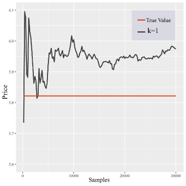
(a) ref1

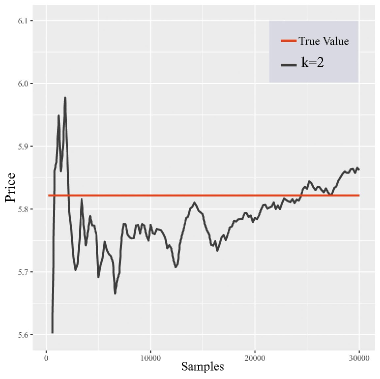
(b) ref2

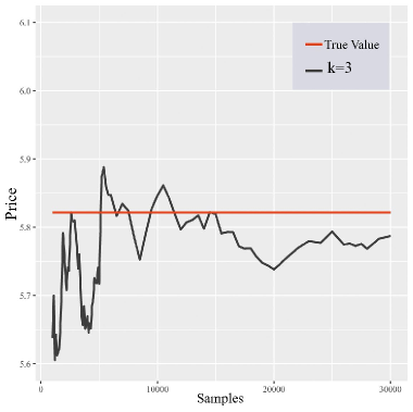
(c) ref3

Figure 1. Monte Carlo experiments for $c^{k,*}$ with $\epsilon_{k}=2^{-k}$

8. Appendix A. Random mesh and large deviations

Lemma 8.1.

For every $q\geq 1$ and $\beta\in(0,1)$, there exists a constant $C$ which depends on $q\geq 1$ and $\beta$ such that

$$\mathbb{E}|\vee_{n\geq 1}\Delta T^{k}_{n}|^{q}\mathds{1}_{\{T^{k}_{n}\leq T\}}\leq C\Big{(}\epsilon_{k}^{2q}\Big{\lceil}\frac{\epsilon^{-2}_{k}T}{\chi_{d}}\Big{\rceil}^{(1-\beta)}\Big{)},$$

for every $k\geq 1$.

Proof.

We start by noticing (see (3.2)) that $\Delta T^{k}_{n}=\min_{j\in\{1,2,\dots,d\}}{\{\Delta T^{k,j}_{n}\}}$ a.s where $\Delta T^{k,j}_{n}\stackrel{{\scriptstyle d}}{{=}}\epsilon_{k}^{2}\tau^{j}_{n}$ for an iid sequence of random variables $(\tau^{j}_{i})_{i\geq 1}$ with distribution equals to $\inf\{t>0;|W^{j}(t)|=1\}$ for a sequence of independent real-valued Brownian motions $(W^{j})_{j=1}^{d}$. We observe there exists $\lambda>0$ such that

(8.1) $$\mathbb{E}\exp(\lambda\min\{\tau^{1}_{1},\ldots,\tau_{1}^{d}\})\leq\mathbb{E}\exp(\lambda\tau^{1}_{1})<\infty.$$

Moreover,

$$\left(\mathbb{E}[(\Delta T^{k}_{1})^{q/(1-\beta)}]\right)^{1-\beta}=\epsilon_{k}^{2q}\left(\mathbb{E}[\min\{\tau^{1},\ldots,\tau^{d}_{1}\}^{q/(1-\beta)}]\right)^{1-\beta}=:C\epsilon_{k}^{2q},$$

Having said that, by applying Lemma 1.1 (Supplementary Material of [41]), the proof is almost identical to Lemma 2.2 in [41], so we omit the details. ∎

Let $I^{*}_{d}$ be the Cramer-Legendre transform of $\min\{\tau^{1},\ldots,\tau^{d}\}$ for the random variables described in (3.8).

Lemma 8.2.

For each $t\in(0,T]$ and $0<\delta<t$, we have

(8.2) $$\lim_{k\rightarrow+\infty}T^{k}_{e(k,t)}=t~{}\text{a.s}$$

and

(8.3) $$\mathbb{P}\Big{\{}T^{k}_{e(k,t)}<t-\delta\Big{\}}\leq\exp\Big{[}-e(k,t)I^{*}_{d}\Big{(}\chi_{d}\Big{(}1-\frac{\delta}{t}\Big{)}\Big{)}\Big{]},$$

for every $k\geq 1$. Moreover, there exists a constant $C$ which depends on $p\geq 1$, $\chi_{d}$ and $t\in[0,T]$ such that

(8.4) $$\mathbb{E}|t-T^{k}_{e(k,t)}|^{p}\leq C\epsilon_{k}^{2p},$$

for every $k\geq 1$.

Proof.

Fix $t\in(0,T]$. Assertion (8.2) is a consequence of the strong law of large numbers, (3.2) and the fact that $\lim_{k\rightarrow+\infty}e(k,t)\epsilon^{2}_{k}\chi_{d}=t$. The estimate (8.3) is a routine application of the classical large deviation principle. Now, we write $\mathbb{E}|T^{k}_{e(k,t)}-t|^{p}=\epsilon^{2p}_{k}\mathbb{E}|\epsilon^{-2}_{k}(T^{k}_{e(k,t)}-t)|^{p}$ and we claim that $\sup_{k\geq 1}\mathbb{E}|\epsilon^{-2}_{k}(T^{k}_{e(k,t)}-t)|^{p}<\infty$. We want to check

(8.5) $$\sup_{k\geq 1}\int_{\{T^{k}_{e(k,t)}>t\}}\big{[}\epsilon^{-2}_{k}(T^{k}_{e(k,t)}-t)\big{]}^{p}d\mathbb{P}+\sup_{k\geq 1}\int_{\{T^{k}_{e(k,t)}\leq t\}}\big{[}\epsilon^{-2}_{k}(t-T^{k}_{e(k,t)}\big{]}^{p}d\mathbb{P}<\infty.$$

Since $\big{[}\epsilon^{-2}_{k}(T^{k}_{e(k,t)}-t)\big{]}^{p}\mathds{1}_{\{T^{k}_{e(k,t)}>t\}}$ is a positive random variable, we have

$$\int_{\{T^{k}_{e(k,t)}>t\}}\big{[}\epsilon^{-2}_{k}(T^{k}_{e(k,t)}-t)\big{]}^{p}d\mathbb{P}\leq\int_{1}^{\infty}\exp\Big{(}-e(k,t)I^{*}_{d}\Big{(}\chi_{d}\frac{t+\epsilon_{k}^{2}s^{1/p}}{t+\epsilon_{k}^{2}\chi_{d}}\Big{)}\Big{)}ds+1,$$

where $s\mapsto I^{*}_{d}\big{(}\chi_{d}\frac{t+\epsilon_{k}^{2}s^{1/p}}{t+\epsilon_{k}^{2}\chi_{d}}\big{)}$ is positive strictly increasing on $[1,\infty)$. Recall that $I^{*}_{d}$ is increasing on $[\chi_{d},\infty)$ and $I^{*}_{d}(\chi_{d})=0$. The analysis for the second term in (8.5) is similar. This shows (8.4). ∎

9. Appendix B. Probability Kernel

In this section, we provide a closed form expression for the probability kernel (5.5) given by

$$\nu^{k}(E)=\mathbb{P}\Big{\{}(\Delta T^{k}_{1},\eta^{k}_{1})\in E\Big{\}};E\in\mathcal{B}(\mathbb{S}_{k}).$$

In the sequel, $f$ is the density function (see e.g [7]) of $\tau=\inf\{t>0;|Y(t)|=1\}$ for a standard Brownian motion $Y$. Formula for $d=1$ is a simple consequence of the strong Markov property of the Brownian motion. For simplicity, we present the formula for $d=2$. The argument for $d>2$ is similar. In the sequel, we consider generic Borel sets of the form $\{(a,b)\times\{\pm\epsilon_{k}\}\times(y,\bar{y})\}$ and $\{(a,b)\times(y,\bar{y})\times\{\pm\epsilon_{k}\}\}$ for arbitrary open sets $(a,b)$ and $(y,\bar{y})\subset(-\epsilon_{k},\epsilon_{k})$. Clearly, this class of sets generates the Borel sigma algebra of $\mathbb{S}_{k}$. The proof of the following formula is lengthy but straightforward, so we omit the details.

Proposition 9.1.

Assume the underlying Brownian motion is $d$-dimensional with $d=2$. For each $a<b$, $\epsilon_{k}>0$ and $-\epsilon_{k}<y<\bar{y}<\epsilon_{k}$, we have

$$\nu^{k}\Big{(}(a,b)\times\{\pm\epsilon_{k}\}\times(y,\bar{y})\Big{)} = \epsilon^{-2}_{k}\int_{y}^{\bar{y}}\int_{0}^{\infty}\frac{1}{\sqrt{2\pi t}}\frac{\exp\left(-\frac{x^{2}}{t}\right)}{2\left(\Phi\left(\frac{\epsilon_{k}}{\sqrt{t}}\right)\right)}f(\epsilon_{k}^{-2}t)dtdx$$

$$\times \frac{1}{2d}\int_{\epsilon_{k}^{-2}a}^{\epsilon_{k}^{-2}b}f(x)dx;k\geq 1.$$

10. Appendix C. Construction of optimal controls: Measurable selection and $\epsilon$-controls

In this section, we provide the proofs of the technical details associated with our dynamic programming algorithm described in Section 5.1. In the sequel, it will be important to deal with universally measurable sets. For readers who are not familiar with this class of sets, we refer to e.g [3]. If $(R,\beta(R))$ is a Borel space, let $P(R)$ be the space of all probability measures defined on the Borel $\sigma$-algebra $\mathcal{B}(R)$ generated by $R$. We denote

$$\mathcal{E}(R):=\bigcap_{p\in P(R)}\mathcal{B}(R,p),$$

where $\mathcal{B}(R,p)$ is the $p$-completion of $\mathcal{B}(R)$ w.r.t $p\in P(R)$.

In the sequel, it will be useful to work with the set $\widetilde{U}^{k,n}_{\ell}$ of all controls $v^{k}:~{}]]T^{k}_{\ell},T^{k}_{n}[[\rightarrow\mathbb{A}$ of the form (3.3) but $v^{k}_{j-1}$ is an $\mathbb{A}$-valued $\widetilde{\mathcal{F}}^{k}_{T^{k}_{j-1}}$-measurable random variable for every $j\in\{\ell+1,\ldots,n\}$ for $0\leq\ell<n<\infty$.

Lemma 10.1.

Let $G^{k}_{j}:\mathbb{H}^{k,j}\rightarrow E$ be a universally measurable function, where $(E,\mathcal{B}(E))$ is a Borel space. Then, the composition $G^{k}_{j}\circ\Xi^{k,u^{k}}_{j}$ is $\mathcal{F}^{k}_{T^{k}_{j}}$-mensurable, for every $u^{k}\in U^{k,e(k,T)}_{0}$ and $j=1,\ldots,m$.

Proof.

We need to show that given $D\in\mathcal{B}(E)$, the inverse image $(\Xi^{k,u^{k}}_{j})^{-1}[(G^{k}_{j})^{-1}(D)]\in\mathcal{F}^{k}_{T^{k}_{j}}$. Since $(G^{k}_{j})^{-1}(D)$ is a universally measurable set, it is sufficient to check that $(\Xi^{k,u^{k}}_{j})^{-1}(H)\in\mathcal{F}^{k}_{T^{k}_{j}}$ for every universally measurable set $H$ in $\mathbb{H}^{k,j}$. Let $\mu$ be a probability measure on $\mathbb{H}^{k,j}$ given by

$$\mu(C)=\mathbb{P}\left[(\Xi^{k,u^{k}}_{j})^{-1}(C)\right],~{}~{}C\in\mathcal{B}(\mathbb{H}^{k,j}).$$

For a given universally measurable set $H$ in $\mathbb{H}^{k,j}$, we can select (see e.g Lemma 7.26 in [3]) $\tilde{H}\in\mathcal{B}(\mathbb{H}^{k,j})$ be such that

$$\mathbb{P}\left[(\Xi^{k,u^{k}}_{j})^{-1}(\tilde{H})\bigtriangleup(\Xi^{k,u^{k}}_{j})^{-1}(H)\right]=\mu\left[\tilde{H}\bigtriangleup H\right]=0.$$

The set $(\Xi^{k,u^{k}}_{j})^{-1}(\tilde{H})\in\mathcal{F}^{k}_{T^{k}_{j}}$, so there exists $W\in\widetilde{\mathcal{F}}^{k}_{T^{k}_{j}}$ such that $\mathbb{P}\left[W\bigtriangleup(\Xi^{k,u^{k}}_{j})^{-1}(\tilde{H})\right]=0$. Then, $\mathbb{P}\left[W\bigtriangleup(\Xi^{k,u^{k}}_{j})^{-1}(H)\right]=0$ and hence, $(\Xi^{k,u^{k}}_{j})^{-1}(H)\in\mathcal{F}^{k}_{T^{k}_{j}}$. This concludes the proof.

∎

Let us now present a selection measurable theorem which will allow us to aggregate the map $u^{k}\mapsto V^{k}(\cdot,u^{k})$ into a single list of upper semi-analytic functions $F^{k}_{j}:\mathbb{H}^{k,j}\rightarrow\mathbb{R};j=0,\ldots,e(k,T)$. To keep notation simple, in the sequel we set $m=e(k,T)$. We fix a structure of the form (4.1) equipped with a Borel function $\gamma^{k}_{m}:\mathbb{H}^{k,m}\rightarrow\mathbf{D}_{T}^{n}$ realizing (5.6) with a given initial condition $x\in\mathbb{R}^{n}$. For such structure, we write $V^{k}$ as the associated value process given by (4.3).

We start with the map $\mathbb{V}^{k}_{m}:\mathbb{H}^{k,m}\rightarrow\mathbb{R}$ defined by

$$\mathbb{V}^{k}_{m}(\textbf{o}^{k}_{m}):=\xi(\gamma^{k}_{m}(\textbf{o}^{k}_{m}));\textbf{o}^{k}_{m}\in\mathbb{H}^{k,m}.$$

By construction, $\mathbb{V}^{k}_{m}$ is a Borel function.

Lemma 10.2.

Assume that $\xi_{X^{k}}(u^{k})\in L^{1}(\mathbb{P})$ for $u^{k}\in U^{k,m}_{0}$. Then,

(10.1) $$\mathbb{E}\left[\xi_{X^{k}}(u^{k})|\mathcal{F}^{k}_{T^{k}_{m-1}}\right]=\int_{\mathbb{S}_{k}}\mathbb{V}^{k}_{m}\left[\Big{(}(u^{k}_{0},\Delta T^{k}_{1},\eta^{k}_{1}),\ldots,(u^{k}_{m-1},s^{k}_{m},\tilde{i}^{k}_{m})\Big{)}\right]\nu^{k}(ds^{k}_{m}d\tilde{i}^{k}_{m})~{}a.s$$

Proof.

At first, we observe

(10.2) $$\mathbb{E}\left[\xi_{X^{k}}(u^{k})|\mathcal{F}^{k}_{T^{k}_{m-1}}\right]=\mathbb{E}\left[\xi_{X^{k}}(u^{k})|\widetilde{\mathcal{F}}^{k}_{T^{k}_{m-1}}\right]\quad a.s$$

for every $u^{k}=(u^{k}_{0},\ldots,u^{k}_{m-1})\in U^{k,m}_{0}$. Elementary computation yields

$$\mathbb{E}\left[\xi_{X^{k}}(u^{k})|\widetilde{\mathcal{F}}^{k}_{T^{k}_{m-1}}\right]=\int_{\mathbb{S}_{k}}\mathbb{V}^{k}_{m}\left[\Big{(}(u^{k}_{0},\Delta T^{k}_{1},\eta^{k}_{1}),\ldots,(u^{k}_{m-1},s^{k}_{m},\tilde{i}^{k}_{m})\Big{)}\right]\nu^{k}(ds^{k}_{m}d\tilde{i}^{k}_{m})~{}a.s$$

for every control $u^{k}=(u^{k}_{0},\ldots,u^{k}_{m-1})\in\widetilde{U}^{k,m}_{0}$. Now, we recall for a given $u^{k}=(u^{k}_{0},\ldots,u^{k}_{m-1})\in U^{k,m}_{0}$, there exists $v^{k}=(v^{k}_{0},\ldots,v^{k}_{m-1})\in\widetilde{U}^{k,m}_{0}$ which fulfills the following: for each $i$, there exists a set $\tilde{G}^{k}_{i}\in\widetilde{\mathcal{F}}^{k}_{T^{k}_{i}}$ of full probability such that $u^{k}_{i}(\omega)=v^{k}_{i}(\omega);\omega\in\tilde{G}^{k}_{i}$ for $i=0,\ldots,m-1$. Let us denote $\tilde{G}^{k}=\cap_{i=0}^{m-1}\widetilde{G}^{k}_{i}\in\widetilde{\mathcal{F}}^{k}_{T^{k}_{m-1}}$. Then, $u^{k}=v^{k}$ in $\tilde{G}^{k}$ and hence

$$\mathbb{E}\left[\xi_{X^{k}}(u^{k})|\widetilde{\mathcal{F}}^{k}_{T^{k}_{m-1}}\right] = \mathbb{E}\left[\xi_{X^{k}}(u^{k})|\widetilde{\mathcal{F}}^{k}_{T^{k}_{m-1}}\right]\mathds{1}_{\{\tilde{G}^{k}\}}=\mathbb{E}\left[\xi_{X^{k}}(v^{k})\mathds{1}_{\{\tilde{G}^{k}\}}|\widetilde{\mathcal{F}}^{k}_{T^{k}_{m-1}}\right]$$

$$= \int_{\mathbb{S}_{k}}\mathds{1}_{\{\tilde{G}^{k}\}}\mathbb{V}^{k}_{m}\left[\Big{(}(v^{k}_{0},\Delta T^{k}_{1},\eta^{k}_{1}),\ldots,(v^{k}_{m-1},s^{k}_{m},\tilde{i}^{k}_{m})\Big{)}\right]\nu^{k}(ds^{k}_{m}d\tilde{i}^{k}_{m})$$

$$= \int_{\mathbb{S}_{k}}\mathds{1}_{\{\tilde{G}^{k}\}}\mathbb{V}^{k}_{m}\left[\Big{(}(u^{k}_{0},\Delta T^{k}_{1},\eta^{k}_{1}),\ldots,(u^{k}_{m-1},s^{k}_{m},\tilde{i}^{k}_{m})\Big{)}\right]\nu^{k}(ds^{k}_{m}d\tilde{i}^{k}_{m})$$

$$= \int_{\mathbb{S}_{k}}\mathbb{V}^{k}_{m}\left[\Big{(}(u^{k}_{0},\Delta T^{k}_{1},\eta^{k}_{1}),\ldots,(u^{k}_{m-1},s^{k}_{m},\tilde{i}^{k}_{m})\Big{)}\right]\nu^{k}(ds^{k}_{m}d\tilde{i}^{k}_{m})~{}a.s.$$

Identities (10.2) and (LABEL:iqual_2) allow us to conclude the proof. ∎

Lemma 10.3.

The map

$$(\mathbf{o}^{k}_{m-1},a^{k}_{m-1})\mapsto\int_{\mathbb{S}_{k}}\mathbb{V}^{k}_{m}\big{(}\mathbf{o}^{k}_{m-1},a^{k}_{m-1},s^{k}_{m},\tilde{i}^{k}_{m}\big{)}\nu^{k}(ds^{k}_{m}d\tilde{i}^{k}_{m})$$

is a Borel function from $\mathbb{H}^{k,m-1}\times\mathbb{A}$ to $\overline{\mathbb{R}}$.

Proof.

We just need to imitate the proof of Prop. 7.29 in ([3]). ∎

Lemma 10.4.

Let $\mathbb{V}^{k}_{m-1}:\mathbb{H}^{k,m-1}\rightarrow\overline{\mathbb{R}}$ be the function defined by

$$\mathbb{V}^{k}_{m-1}(\mathbf{o}^{k}_{m-1}):=\sup_{a^{k}_{m-1}\in\mathbb{A}}\int_{\mathbb{S}_{k}}\mathbb{V}^{k}_{m}\big{(}\mathbf{o}^{k}_{m-1},a^{k}_{m-1},s^{k}_{m},\tilde{i}^{k}_{m}\big{)}\nu^{k}(ds^{k}_{m}d\tilde{i}^{k}_{m}),$$

for $\mathbf{o}^{k}_{m-1}\in\mathbb{H}^{k,m-1}$. Then, $\mathbb{V}^{k}_{m-1}$ is upper semianalytic and for every $\epsilon>0$, there exists an analytically measurable function $C^{\epsilon}_{k,m-1}:\mathbb{H}^{k,m-1}\rightarrow\mathbb{A}$ which realizes

(10.4) $$\mathbb{V}^{k}_{m-1}(\mathbf{o}^{k}_{m-1})\leq\int_{\mathbb{S}_{k}}\mathbb{V}^{k}_{m}\big{(}\mathbf{o}^{k}_{m-1},C^{\epsilon}_{k,m-1}(\mathbf{o}^{k}_{m-1}),s^{k}_{m},\tilde{i}^{k}_{m}\big{)}\nu^{k}(ds^{k}_{m}d\tilde{i}^{k}_{m})+\epsilon,$$

for every $\mathbf{o}^{k}_{m-1}\in\{\mathbb{V}^{k}_{m-1}<+\infty\}$.

Proof.

The fact that $\mathbb{V}^{k}_{m-1}$ is upper semianalytic follows from Prop 7.47 in [3] and Lemma 10.3 which say the map given by

$$f(\mathbf{o}^{k}_{m-1},a^{k}_{m-1})=\int_{\mathbb{S}_{k}}\mathbb{V}^{k}_{m}\big{(}\mathbf{o}^{k}_{m-1},a^{k}_{m-1},s^{k}_{m},\tilde{i}^{k}_{m}\big{)}\nu^{k}(ds^{k}_{m}d\tilde{i}^{k}_{m})$$

is a Borel function (hence upper semianalytic). Moreover, by construction, $\mathbb{H}^{k,m-1}\times\mathbb{A}$ is a Borel set. Let

$$\mathbb{V}^{k}_{m-1}(\mathbf{o}^{k}_{m-1})=\sup_{a^{k}_{m-1}\in\mathbb{A}}f(\mathbf{o}^{k}_{m-1},a^{k}_{m-1});\mathbf{o}^{k}_{m-1}\in\mathbb{H}^{k,m-1}.$$

Prop 7.50 in [3] yields the existence of an analytically measurable function $C^{\epsilon}_{k,m-1}:\mathbb{H}^{k,m-1}\rightarrow\mathbb{A}$ such that

$$f\big{(}\mathbf{o}^{k}_{m-1},C^{\epsilon}_{k,m-1}(\mathbf{o}^{k}_{m-1})\big{)}\geq\mathbb{V}^{k}_{m-1}(\mathbf{o}^{k}_{m-1})-\epsilon,$$

for every $\mathbf{o}^{k}_{m-1}\in\{\mathbb{V}^{k}_{m-1}<+\infty\}$. ∎

Lemma 10.5.

If $\mathbb{H}^{k}_{m-1}=\{\mathbb{V}^{k}_{m-1}<+\infty\}$, then for every $\epsilon>0$ and $u^{k}\in U^{k,m}_{0}$, there exists a control $\phi^{k,\epsilon}_{m-1}\in U^{k,m}_{m-1}$ such that

(10.5) $$\mathbb{V}^{k}_{m-1}(\Xi^{k,u^{k}}_{m-1})=V^{k}(T^{k}_{m-1},u^{k})\leq\mathbb{E}\big{[}V^{k}(T^{k}_{m},u^{k}\otimes_{m-1}\phi^{k,\epsilon}_{m-1})|\mathcal{F}^{k}_{T^{k}_{m-1}}\big{]}+\epsilon~{}a.s.$$

Proof.

For every $\theta^{k}_{m-1}\in U^{k,m}_{m-1}$, it follows from Equation (10.1) that $\mathbb{E}\big{[}\xi_{X^{k}}(u^{k}\otimes_{m-1}\theta^{k}_{m-1})|\mathcal{F}^{k}_{T^{k}_{m-1}}\big{]}$ equals (a.s) to

$$\int_{\mathbb{S}_{k}}\mathbb{V}^{k}_{m}\left[\Big{(}(u^{k}_{0},\Delta T^{k}_{1},\eta^{k}_{1}),\ldots,(u^{k}_{m-2},\Delta T^{k}_{m-1},\eta^{k}_{m-1}),(\theta^{k}_{m-1},s^{k}_{m},\tilde{i}^{k}_{m})\Big{)}\right]\nu^{k}(ds^{k}_{m}d\tilde{i}^{k}_{m}).$$

As a consequence, we obtain that

(10.6) $$\mathbb{V}^{k}_{m-1}(\Xi^{k,u^{k}}_{m-1})\geq\mathbb{E}\big{[}\xi_{X^{k}}(u^{k}\otimes_{m-1}\theta^{k}_{m-1})|\mathcal{F}^{k}_{T^{k}_{m-1}}\big{]}~{}a.s,$$

for every $\theta^{k}_{m-1}\in U^{k,m}_{m-1}$. By composing $\mathbb{V}^{k}_{m-1}$ with $\Xi^{k,u^{k}}_{m-1}$ in (10.4), we obtain that $\mathbb{V}^{k}_{m-1}(\Xi^{k,u^{k}}_{m-1})$ is an $\mathcal{F}^{k}_{T^{k}_{m-1}}$-measurable function (see, Lemma 10.1). Then, the definition of $\operatorname*{ess\,sup}$ and Equation (10.6) yield that

(10.7) $$\mathbb{V}^{k}_{m-1}(\Xi^{k,u^{k}}_{m-1})\geq\operatorname*{ess\,sup}_{\theta^{k}_{m-1}\in U^{k,m}_{m-1}}\mathbb{E}\Bigg{[}V^{k}\left(T^{k}_{m},u^{k,m-1}\otimes_{m-1}\theta^{k}_{m-1}\right)\mid\mathcal{F}^{k}_{T^{k}_{m-1}}\Bigg{]}=V^{k}(T^{k}_{m-1},u^{k})~{}a.s.$$

For $\epsilon>0$, let $C^{\epsilon}_{k,m-1}:\mathbb{H}^{k,m-1}\rightarrow\mathbb{A}$ be the analytically measurable function which realizes (10.4). We take $\phi^{k,\epsilon}_{m-1}:=C^{\epsilon}_{k,m-1}(\Xi^{k,u^{k}}_{m-1})$ as the composition of an analytically measurable function with an $\mathcal{F}^{k}_{T^{k}_{m-1}}$-measurable one. In this case, by Lemma 10.1, we know that $C^{\epsilon}_{k,m-1}\circ\Xi^{k,u^{k}}_{m-1}$ is an $\mathcal{F}^{k}_{T^{k}_{m-1}}$-measurable function. This shows that $\phi^{k,\epsilon}_{m-1}$ is an admissible control. It follows from (10.4) that

$$\mathbb{V}^{k}_{m-1}(\Xi^{k,u^{k}}_{m-1}) \leq \int_{\mathbb{S}_{k}}\mathbb{V}^{k}_{m}\left[\Big{(}(u^{k}_{0},\Delta T^{k}_{1},\eta^{k}_{1}),\ldots,(u^{k}_{m-2},\Delta T^{k}_{m-1},\eta^{k}_{m-1}),(\phi^{k,\epsilon}_{m-1},s^{k}_{m},\tilde{i}^{k}_{m})\Big{)}\right]\nu^{k}(ds^{k}_{m}d\tilde{i}^{k}_{m})+\epsilon$$

$$= \mathbb{E}\big{[}\xi_{X^{k}}(u^{k}\otimes_{m-1}\phi^{k,\epsilon}_{m-1})|\mathcal{F}^{k}_{T^{k}_{m-1}}\big{]}+\epsilon=\mathbb{E}\big{[}V^{k}(T^{k}_{m},u^{k}\otimes_{m-1}\phi^{k,\epsilon}_{m-1})|\mathcal{F}^{k}_{T^{k}_{m-1}}\big{]}+\epsilon$$

$$\leq \operatorname*{ess\,sup}_{\theta^{k}_{m-1}\in U^{k,m}_{m-1}}\mathbb{E}\Bigg{[}V^{k}\left(T^{k}_{m},u^{k,m-1}\otimes_{m-1}\theta^{k}_{m-1}\right)\mid\mathcal{F}^{k}_{T^{k}_{m-1}}\Bigg{]}+\epsilon~{}~{}a.s.$$

As $\epsilon>0$ is arbitrary, we conclude that

(10.9) $$\mathbb{V}^{k}_{m-1}(\Xi^{k,u^{k}}_{m-1})\leq\operatorname*{ess\,sup}_{\theta^{k}_{m-1}\in U^{k,m}_{m-1}}\mathbb{E}\Bigg{[}V^{k}\left(T^{k}_{m},u^{k,m-1}\otimes_{m-1}\theta^{k}_{m-1}\right)\mid\mathcal{F}^{k}_{T^{k}_{m-1}}\Bigg{]}=V^{k}(T^{k}_{m-1},u^{k})~{}a.s.$$

Hence, it follows from Equations (10.7) and (10.9) that

$$\mathbb{V}^{k}_{m-1}(\Xi^{k,u^{k}}_{m-1})=V^{k}(T^{k}_{m-1},u^{k})~{}a.s,~{}~{}u^{k}\in U^{k,m}_{0}.$$

Moreover, as a consequence of Equation (LABEL:Ineq_3), we obtain that

$$V^{k}(T^{k}_{m-1},u^{k})=\mathbb{V}^{k}_{m-1}(\Xi^{k,u^{k}}_{m-1})\leq\mathbb{E}\big{[}V^{k}(T^{k}_{m},u^{k}\otimes_{m-1}\phi^{k,\epsilon}_{m-1})|\mathcal{F}^{k}_{T^{k}_{m-1}}\big{]}+\epsilon~{}a.s.$$

∎

We are now able to iterate the argument as follows. From a backward argument, we can define the sequence of functions $\mathbb{V}^{k}_{\ell}:\mathbb{H}^{k,\ell}\rightarrow\overline{\mathbb{R}}$

(10.10) $$\mathbb{V}^{k}_{\ell}(\mathbf{o}^{k}_{\ell}):=\sup_{a^{k}_{\ell}\in\mathbb{A}}\int_{\mathbb{S}_{k}}\mathbb{V}^{k}_{\ell+1}(\mathbf{o}^{k}_{\ell},a^{k}_{\ell},s^{k}_{\ell+1},\tilde{i}^{k}_{\ell+1})\nu^{k}(ds^{k}_{\ell+1}d\tilde{i}^{k}_{\ell+1}),$$

for $\mathbf{o}^{k}_{\ell}\in\mathbb{H}^{k,\ell}$ and $\ell=m-1,\ldots,1$.

Remark 10.1.

One can easily check that if $Y=h(\mathcal{A}^{k}_{r})$, then

$$\mathbb{E}[Y|\mathcal{A}^{k}_{j-1}]=\int_{\mathbb{S}^{r-j+1}_{k}}h(\mathcal{A}^{k}_{j-1},x_{j},\ldots,x_{r})\mathbb{P}^{k}_{r-j+1}(dx_{j}\ldots dx_{r})$$

for $j=1,\ldots,r$.

Lemma 10.6.

For each $j=m-1,\ldots,1$, the map

$$(\mathbf{o}^{k}_{j},a^{k}_{j})\mapsto\int_{\mathbb{S}_{k}}\mathbb{V}^{k}_{j+1}(\mathbf{o}^{k}_{j},a^{k}_{j},s^{k}_{j+1},\tilde{i}^{k}_{j+1})\nu^{k}(ds^{k}_{j+1}d\tilde{i}^{k}_{j+1})$$

is upper semianalytic from $\mathbb{H}^{k,j}\times\mathbb{A}$ to $\overline{\mathbb{R}}$.

Proof.

The same argument used in the proof of Lemma 10.3 applies here. We omit the details. ∎

Proposition 10.1.

The function $\mathbb{V}^{k}_{j}:\mathbb{H}^{k,j}\rightarrow\overline{\mathbb{R}}$ is upper semianalytic for each $j=m-1,\ldots,1$. Moreover, for every $\epsilon>0$, there exists an analytically measurable function $C^{\epsilon}_{k,j}:\mathbb{H}^{k,j}\rightarrow\mathbb{A}$ such that

(10.11) $$\mathbb{V}^{k}_{j}(\mathbf{o}^{k}_{j})\leq\int_{\mathbb{S}_{k}}\mathbb{V}^{k}_{j+1}\big{(}\mathbf{o}^{k}_{j},C^{\epsilon}_{k,j}(\mathbf{o}^{k}_{j}),s^{k}_{j+1},\tilde{i}^{k}_{j+1}\big{)}\nu^{k}(ds^{k}_{j+1}d\tilde{i}^{k}_{j+1})+\epsilon,$$

for every $\mathbf{o}^{k}_{j}\in\{\mathbb{V}^{k}_{j}<+\infty\}$, where $j=m-1,\ldots,1$.

Proof.

We just repeat the argument of the proof of Lemma 10.4 jointly with Lemma 10.6. ∎

We are now able to define the value function at step $j=0$ as follows

$$\mathbb{V}^{k}_{0}:=\sup_{a^{k}_{0}\in\mathbb{A}}\int_{\mathbb{S}_{k}}\mathbb{V}^{k}_{1}(a^{k}_{0},s^{k}_{1},\tilde{i}^{k}_{1})\nu^{k}(ds^{k}_{1}d\tilde{i}^{k}_{1}).$$

Therefore, if $\mathbb{V}^{k}_{0}<+\infty$ then for $\epsilon>0$, there exists $C^{\epsilon}_{k,0}\in\mathbb{A}$ which realizes

$$\mathbb{V}^{k}_{0}<\int_{\mathbb{S}_{k}}\mathbb{V}^{k}_{1}\big{(}C^{\epsilon}_{k,0},s^{k}_{1},\tilde{i}^{k}_{1}\big{)}\nu^{k}(ds^{k}_{1}d\tilde{i}^{k}_{1})+\epsilon.$$

Proposition 10.2.

For each $j=m-1,\ldots,0$ and a control $u^{k}\in U^{k,m}_{0}$, we have

(10.12) $$\mathbb{V}^{k}_{j}(\Xi^{k,u^{k}}_{j})=V^{k}(T^{k}_{j},u^{k})~{}a.s.$$

Let $C^{\epsilon}_{k,j}:\mathbb{H}^{k,j}\rightarrow\mathbb{A};j=m-1,\ldots,0$ be the functions given in Proposition 10.1. Observe that $C^{\epsilon}_{k,j}$ can be computed from (10.10) and (10.11). If $\mathbb{H}^{k,j}=\{\mathbb{V}^{k}_{j}<+\infty\}$, for $j=m-1,\ldots,0$, then for every $\epsilon>0$, there exists a control $u^{k,\epsilon}_{j}$ defined by

(10.13) $$u^{k,\epsilon}_{j}:=C^{\epsilon}_{k,j}(\Xi^{k,u^{k}}_{j});j=m-1,\ldots,0$$

which realizes

(10.14) $$V^{k}(T^{k}_{j},u^{k})\leq\mathbb{E}\big{[}V^{k}(T^{k}_{j+1},u^{k}\otimes_{j}u^{k,\epsilon}_{j})|\mathcal{F}^{k}_{T^{k}_{j}}\big{]}+\epsilon~{}a.s,$$

for every $j=m-1,\ldots,0$.

Proof.

The statements for $j=m-1$ hold true due to (10.5) in Lemma 10.5. Now, by using Proposition 10.1 and a backward induction argument, we conclude the proof. ∎

We are now able to construct an $\epsilon$-optimal control in this discrete level.

Proposition 10.3.

Let $(\xi,(X^{k})_{k\geq 1})$ be an admissible pair w.r.t the control problem (4.8). Then, $\phi^{*,k,\epsilon}=(\phi^{k,\eta_{k}(\epsilon)}_{0},\phi^{k,\eta_{k}(\epsilon)}_{1},\ldots,\phi^{k,\eta_{k}(\epsilon)}_{m-1})$ constructed via (10.13) is $\epsilon$-optimal, where $\eta_{k}(\epsilon)=\frac{\epsilon}{e(k,T)}$. In other words, for every $\epsilon>0$ and $k\geq 1$, the control $\phi^{*,k,\epsilon}\in U^{k,m}_{0}$ realizes

(10.15) $$\sup_{u^{k}\in U^{k,m}_{0}}\mathbb{E}\big{[}\xi_{X^{k}}(u^{k})\big{]}\leq\mathbb{E}\big{[}\xi_{X^{k}}(\phi^{*,k,\epsilon})\big{]}+\epsilon.$$

Proof.

Fix $\epsilon>0$ and let $\eta_{k}(\epsilon)=\frac{\epsilon}{m}$, where we recall $m=e(k,T)$. The candidate for an $\epsilon$-optimal control is

$$\phi^{*,k,\epsilon}=(\phi^{k,\eta_{k}(\epsilon)}_{0},\phi^{k,\eta_{k}(\epsilon)}_{1},\ldots,\phi^{k,\eta_{k}(\epsilon)}_{m-1}),$$

where $\phi^{k,\eta_{k}(\epsilon)}_{i};i=m-1,\ldots,0$ are constructed via (10.13). Let us check it is indeed $\epsilon$-optimal. From (10.14), we know that

(10.16) $$\sup_{u^{k}\in U^{k,e(k,T)}_{0}}\mathbb{E}\big{[}\xi_{X^{k}}(u^{k})\big{]}\leq\mathbb{E}\big{[}V^{k}(T^{k}_{1},\phi^{k,\eta_{k}(\epsilon)}_{0})\big{]}+\eta_{k}(\epsilon)$$

and

(10.17) $$V^{k}(T^{k}_{1},\phi^{k,\eta_{k}(\epsilon)}_{0})\leq\mathbb{E}\big{[}V^{k}(T^{k}_{2},\phi^{k,\eta_{k}(\epsilon)}_{0}\otimes_{1}\phi^{k,\eta_{k}(\epsilon)}_{1})|\mathcal{F}^{k}_{T^{k}_{1}}\big{]}+\eta_{k}(\epsilon)~{}a.s.$$

Inequalities (10.16) and (10.17) yield

(10.18) $$\sup_{u^{k}\in U^{k,e(k,T)}_{0}}\mathbb{E}\big{[}\xi_{X^{k}}(u^{k})\big{]}\leq\mathbb{E}\big{[}V^{k}(T^{k}_{2},\phi^{k,\eta_{k}(\epsilon)}_{0}\otimes_{1}\phi^{k,\eta_{k}(\epsilon)}_{1})\big{]}+2\eta_{k}(\epsilon),$$

where (10.14) implies $V^{k}(T^{k}_{j},\phi^{k,\eta_{k}(\epsilon)}_{0}\otimes_{1}\phi^{k,\eta_{k}(\epsilon)}_{1}\otimes_{2}\ldots\otimes_{j-1}\phi^{k,\eta_{k}(\epsilon)}_{j-1})$ is less than or equals to

(10.19) $$\mathbb{E}\big{[}V^{k}(T^{k}_{j+1},\phi^{k,\eta_{k}(\epsilon)}_{0}\otimes_{1}\phi^{k,\eta_{k}(\epsilon)}_{1}\otimes_{2}\ldots\otimes_{j}\phi^{k,\eta_{k}(\epsilon)}_{j})|\mathcal{F}^{k}_{T^{k}_{j}}\big{]}+\eta_{k}(\epsilon)~{}a.s,$$

for $j=1,\ldots,m-1$. By iterating the argument starting from (10.18) and using (10.19), we conclude (10.15). ∎

11. Appendix D. Proof of Theorems 5.1 and 5.2

In this section, we provide the proof of Theorems 5.1 and 5.2. The argument is divided into two parts. At first, we will prove it is possible to enlarge the set $U^{k,e(k,T)}_{0}$ to $\overline{U}^{k,e(k,T)}_{0}$ without affecting $V^{k}(0)$. Secondly, we will establish an equiconvergence result for the family of Brownian martingales parameterized by $U^{T}_{0}$. Finally, we invoke the property of the strongly controlled Wiener functionals as demonstrated in Section 6 for a variety of examples.

Since $T^{k}_{n}<\infty$ a.s for each $n\geq 1$, it is known (see e.g. Corollary 3.22 in [27]) that $(\hat{\Phi}^{k}_{j})^{-1}\big{(}\mathcal{O}\big{)}=\mathcal{F}_{T^{k}_{j}}$, where $\mathcal{O}$ is the optional $\sigma$-algebra on $\Omega\times\mathbb{R}_{+}$ and

$$\hat{\Phi}^{k}_{j}(\omega):=\Phi^{k}_{j}(\omega,T^{k}_{j}(\omega)):=\big{(}\omega,T^{k}_{j}(\omega)\big{)};\omega\in\Omega^{*},~{}j\geq 1,$$

where $\mathbb{P}(\Omega^{*})=1$. To keep notation simple, we choose a version of $\Phi^{k}_{j}$ defined everywhere and with a slight abuse of notation we write it as $\Phi^{k}_{j}$. Based on this fact, for each $\mathbb{A}$-valued and $\mathcal{F}_{T^{k}_{\ell}}$-measurable variable $v^{k}_{\ell};\ell=e(k,T)-1,\ldots,n$, there exists a list of Borel functions $\varphi^{k}_{\ell}:\Omega\times\mathbb{R}_{+}\rightarrow\mathbb{A}$ which realizes

(11.1) $$v^{k}_{\ell}=\varphi^{k}_{\ell}(\hat{\Phi}^{k}_{\ell})~{}a.s,$$

for $\ell=e(k,T)-1,\ldots,n$. In the sequel, in order to keep notation simple, we set $m=e(k,T)$. For a given $u^{k}\in U^{k,n}_{0}$ and a list of Borel functions $(\varphi^{k}_{\ell})_{\ell=n}^{e(k,T)-1}$ realizing (11.1), we then define the map $\Xi^{k,u^{k}\otimes_{n}\varphi^{k}}_{m}:\Omega\times\mathbb{R}^{m-n}_{+}\times\mathbb{S}^{m}_{k}\rightarrow\mathbb{H}^{k,n}\times\mathbb{H}^{k,m-n}:~{}(\omega,x_{n},\ldots,x_{m-1},\mathbf{b}^{k}_{m})\mapsto\Xi^{k,u^{k}\otimes_{n}\varphi^{k}}_{m}(\omega,x_{n},\ldots,x_{m-1},\mathbf{b}^{k}_{m})$ given by

$$\Big{(}\Xi^{k,u^{k}}_{n}\big{(}\omega\big{)},\varphi^{k}_{n}\big{(}\Phi^{k}_{n}(\omega,x_{n})\big{)},s^{k}_{n+1},\tilde{i}^{k}_{n+1},\ldots,\varphi^{k}_{m-1}\big{(}\Phi^{k}_{m-1}(\omega,x_{m-1})\big{)},s^{k}_{m},\tilde{i}^{k}_{m}\Big{)},$$

for $\omega\in\Omega,(x_{n},\ldots,x_{m-1})\in\mathbb{R}^{m-n}_{+}$ and $\textbf{b}^{k}_{m}\in\mathbb{S}^{m}_{k}$. Let us define

$$J^{k}_{n,m}:=\big{(}\text{Id},T^{k}_{n},\ldots,T^{k}_{m-1},\mathcal{A}^{k}_{m}\big{)},$$

where $\text{Id}:\Omega\rightarrow\Omega$ is the identity map. For each $\bar{\phi}^{k}=(v^{k}_{n},\ldots,v^{k}_{m-1})\in\overline{U}^{k,m}_{n}$ represented by Borel functions $\varphi^{k}_{n},\ldots,\varphi^{k}_{m-1}$ realizing (11.1) and $u^{k}\in U^{k,n}_{0}$, we can represent

$$\xi_{X^{k}}\big{(}u^{k}\otimes_{n}\bar{\phi}^{k}\big{)}=\xi\circ\gamma^{k}_{m}\big{(}\Xi_{m}^{k,u^{k}\otimes_{n}\varphi^{k}}(J^{k}_{n,m})\big{)};n=m-1,\ldots,0$$

where $\gamma^{k}_{m}$ is a pathwise representation for a structure $\mathcal{X}=\big{(}(X^{k})_{k\geq 1},\mathscr{D}\big{)}$.

Let $H^{k}_{n,m}:\mathcal{B}(\Omega\times\mathbb{R}^{m-n+1}_{+})\times\mathbb{S}^{m}_{k}\rightarrow[0,1]$ be the disintegration of $\mathbb{P}\circ J^{k}_{n,m}$ w.r.t $\mathbb{P}^{k}_{m}$ and let $\nu^{k}_{n,m}$ be the disintegration of $\mathbb{P}^{k}_{m}$ w.r.t $\mathbb{P}^{k}_{n}$ for $n=m-1,\ldots,1$. In the sequel, $q^{k}_{n,r}$ is the projection of $\textbf{b}^{k}_{r}$ onto the last $(r-n)$ components. The proof of the following result is elementary, so we omit the details.

Lemma 11.1.

Let $u^{k}\in U^{k,n}_{0}$ and let $\bar{\phi}^{k}=(v^{k}_{n},\ldots,v^{k}_{m-1})\in\overline{U}^{k,m}_{n}$ be a control associated with Borel functions $(\varphi^{k}_{j})_{j=n}^{m-1}$ realizing (11.1) for $n=m-1,\ldots,0$ and $m=e(k,T)$. If $\xi_{X^{k}}(u^{k}\otimes_{n}\bar{\phi}^{k})\in L^{1}(\mathbb{P})$, then

$$\mathbb{E}\Big{[}\xi_{X^{k}}(u^{k}\otimes_{n}\bar{\phi}^{k})|\mathcal{F}^{k}_{T^{k}_{n}}\Big{]}=\int_{\mathbb{S}^{m-n}_{k}}\int_{\Omega\times\mathbb{R}^{m-n}_{+}}\xi\circ\gamma^{k}_{m}\Big{(}\Xi^{k,u^{k}\otimes_{n}\varphi^{k}}_{m}\big{(}\omega,x_{n},\ldots,x_{m-1},\mathcal{A}^{k}_{n},q^{k}_{n,m}\big{)}\Big{)}$$

$$\times H^{k}_{n,m}(d\omega dx_{n}\ldots dx_{m-1}|\mathcal{A}^{k}_{n},q^{k}_{n,m})\nu^{k}_{n,m}(dq^{k}_{n,m}|\mathcal{A}^{k}_{n})~{}a.s.$$

If $\phi^{k}\in U^{k,m}_{n}$ and $\xi_{X^{k}}(u^{k}\otimes_{n}\phi^{k})\in L^{1}(\mathbb{P})$, then we can represent

$$\mathbb{E}\Big{[}\xi_{X^{k}}(u^{k}\otimes_{n}\phi^{k})|\mathcal{F}^{k}_{T^{k}_{n}}\Big{]}=\int_{\mathbb{S}^{m-n}_{k}}\xi\circ\gamma^{k}_{m}\Big{(}\Xi^{k,\widetilde{u}^{k}\otimes_{n}\widetilde{\phi}^{k}}_{m}\big{(}\mathcal{A}^{k}_{n},q^{k}_{n,m}\big{)}\Big{)}\nu^{k}_{n,m}(dq^{k}_{n,m}|\mathcal{A}^{k}_{n})~{}a.s,$$

where $\widetilde{u}^{k}\in\widetilde{U}^{k,n}_{0}$ and $\widetilde{\phi}^{k}\in\widetilde{U}^{k,m}_{n}$ are versions of $u^{k}$ and $\phi^{k}$, respectively.

The following result shows the set of controls $\overline{U}^{k,e(k,T)}_{0}$ and $U^{k,e(k,T)}_{0}$ are equivalent in a suitable sense.

Lemma 11.2.

For $m=e(k,T)$ and $k\geq 1$, we have

(11.2) $$\sup_{\bar{\phi}^{k}\in\overline{U}^{k,m}_{0}}\mathbb{E}\big{[}\xi_{X^{k}}(\bar{\phi}^{k})\big{]} = \sup_{\phi^{k}\in U^{k,m}_{0}}\mathbb{E}\big{[}\xi_{X^{k}}(\phi^{k})\big{]}$$

$$= \sup_{a^{k}_{0},\ldots,a^{k}_{m-1}\in\mathbb{A}^{m}}\int_{\mathbb{S}^{m}_{k}}\xi\circ\gamma^{k}_{m}(a^{k}_{0},s^{k}_{1},\tilde{i}^{k}_{1},\ldots,a^{k}_{m-1},s^{k}_{m},\tilde{i}^{k}_{m})\mathbb{P}^{k}_{m}(d\mathbf{b}^{k}_{m}).$$

Proof.

Following the same argument employed in the proof of Lemma 10.2, we have

$$\sup_{\phi^{k}\in U^{k,m}_{0}}\mathbb{E}\big{[}\xi_{X^{k}}(\phi^{k})\big{]}=\sup_{\phi^{k}\in\widetilde{U}^{k,m}_{0}}\mathbb{E}\big{[}\xi_{X^{k}}(\phi^{k})\big{]}.$$

We now want to check $\sup_{\phi^{k}\in\widetilde{U}^{k,m}_{0}}\mathbb{E}\big{[}\xi_{X^{k}}(\phi)\big{]}$ equals to the expression (11.2). For a given control $u^{k}\in\widetilde{U}^{k,m}_{0}$, let $g^{k}$ be a list of Borel functions such that

$$g^{k}(\mathcal{A}^{k}_{j})=u^{k}_{j};j=0,\ldots,m-1.$$

Let us define $\Xi^{k,g^{k}}_{j}:\mathbb{S}^{j}_{k}\rightarrow\mathbb{H}^{k,j}$

$$\Xi^{k,g^{k}}_{j}\big{(}s^{k}_{1},\tilde{i}^{k}_{1},\ldots,s^{k}_{j},\tilde{i}^{k}_{j}\big{)}:=\Big{(}(g^{k}_{0},s^{k}_{1},\tilde{i}^{k}_{1}),\ldots,(g^{k}_{j-1}(s^{k}_{1},\tilde{i}^{k}_{1},\ldots,s^{k}_{j-1},\tilde{i}^{k}_{j-1}),s^{k}_{j},\tilde{i}^{k}_{j})\Big{)},$$

where $1\leq j\leq m$. Let $\bar{\phi}^{k}=(v^{k}_{n},\ldots,v^{k}_{m-1})\in\overline{U}^{k,m}_{n}$ be a control associated with Borel functions $(\varphi^{k}_{j})_{j=n}^{m-1}$ realizing (11.1) for $n=m-1,\ldots,0$. Moreover, we define the map $\Xi^{k,g^{k}\otimes_{n}\varphi^{k}}_{m}:\Omega\times\mathbb{R}^{m-n}_{+}\times\mathbb{S}^{m}_{k}\rightarrow\mathbb{H}^{k,n}\times\mathbb{H}^{k,m-n}:~{}(\omega,x_{n},\ldots,x_{m-1},\mathbf{b}^{k}_{m})\mapsto\Xi^{k,g^{k}\otimes_{n}\varphi^{k}}_{m}(\omega,x_{n},\ldots,x_{m-1},\mathbf{b}^{k}_{m})$ given by

$$\Big{(}\Xi^{k,g^{k}}_{n}\big{(}\mathbf{b}^{k}_{n}\big{)},\varphi^{k}_{n}\big{(}\Phi^{k}_{n}(\omega,x_{n})\big{)},\ldots,\varphi^{k}_{m-1}\big{(}\Phi^{k}_{m-1}(\omega,x_{m-1})\big{)},s^{k}_{m},\tilde{i}^{k}_{m}\Big{)},$$

for $\omega\in\Omega,(x_{n},\ldots,x_{m-1})\in\mathbb{R}^{m-n}_{+}$ and $\textbf{b}^{k}_{m}\in\mathbb{S}^{m}_{k}$. We define $\overline{V}^{k}(T^{k}_{m},u^{k}):=\xi_{X^{k}}(u^{k})$ and

$$\overline{V}^{k}(T^{k}_{n},u^{k}):=\operatorname*{ess\,sup}_{\bar{\phi}^{k}\in\overline{U}^{k,m}_{n}}\mathbb{E}\Big{[}\xi_{X^{k}}(u^{k}\otimes_{n}\bar{\phi}^{k})|\mathcal{F}^{k}_{T^{k}_{n}}\Big{]};n=m-1,\ldots,1$$

with initial condition $\overline{V}^{k}(0):=\sup_{\bar{\phi}^{k}\in\overline{U}^{k,m}_{0}}\mathbb{E}\big{[}\xi_{X^{k}}(\bar{\phi}^{k})\big{]}$.

By Lemma 11.1,

$$\overline{V}^{k}(T^{k}_{n},u^{k})=\operatorname*{ess\,sup}_{\varphi^{k}}\int_{\mathbb{S}^{m-n}_{k}}\int_{\Omega\times\mathbb{R}^{m-n}_{+}}\xi\circ\gamma^{k}_{m}\Big{(}\Xi^{k,u^{k}\otimes_{n}\varphi^{k}}_{m}\big{(}\omega,x_{n},\ldots,x_{m-1},\mathcal{A}^{k}_{n},q^{k}_{n,m}\big{)}\Big{)}$$

$$\times H^{k}_{n,m}(d\omega dx_{n}\ldots dx_{m-1}|\mathcal{A}^{k}_{n},q^{k}_{n,m})\nu^{k}_{n,m}(dq^{k}_{n,m}|\mathcal{A}^{k}_{n})~{}a.s,$$

where the esssup is computed over the set of all Borel functions $\varphi^{k}_{\ell}:\Omega\times\mathbb{R}_{+}\rightarrow\mathbb{A};\ell=m-1,\ldots,n$ for $n=m-1,\ldots,0$. Now, we define $\overline{\mathbb{V}}^{k}_{n}:\mathbb{H}^{k,n}\rightarrow\overline{\mathbb{R}}$ by

(11.3) $$\overline{\mathbb{V}}^{k}_{n}(\mathbf{o}^{k}_{n}) := \sup_{a^{k}_{n},\ldots,a^{k}_{m-1}\in\mathbb{A}^{m-n}}\int_{\mathbb{S}^{m-n}_{k}}\int_{\Omega\times\mathbb{R}^{m-n}_{+}}\xi\circ\gamma^{k}_{m}\Big{(}\Xi^{k,g^{k}}_{n}(\mathbf{b}^{k}_{n}),a^{k}_{n},\ldots,a^{k}_{m-1},q^{k}_{n,m}\big{)}\Big{)}$$

$$\times H^{k}_{n,m}(d\omega dx_{n}\ldots dx_{m-1}|\mathbf{b}^{k}_{n},q^{k}_{n,m})\nu^{k}_{n,m}(dq^{k}_{n,m}|\mathbf{b}^{k}_{n})$$

$$= \sup_{a^{k}_{n},\ldots,a^{k}_{m-1}\in\mathbb{A}^{m-n}}\int_{\mathbb{S}^{m-n}_{k}}\xi\circ\gamma^{k}_{m}\Big{(}\Xi^{k,g^{k}}_{n}(\mathbf{b}^{k}_{n}),a^{k}_{n},\ldots,a^{k}_{m-1},q^{k}_{n,m}\big{)}\Big{)}\nu^{k}_{n,m}(dq^{k}_{n,m}|\mathbf{b}^{k}_{n}).$$

By construction,

(11.4) $$\overline{\mathbb{V}}^{k}_{n}(\Xi^{k,g^{k}}_{n}(\mathcal{A}^{k}_{n})) = \overline{V}^{k}(T^{k}_{n},u^{k})$$

$$= V^{k}(T^{k}_{n},u^{k})~{}a.s,$$

for $n=m-1,\ldots,0$, where (11.4) is due to (11.3). This concludes the proof of (11.2). ∎

11.1. Equiconvergence of martingales

Let $\mathcal{S}$ be the set of all stepwise constant processes of the form

(11.5) $$Z=Z(0)\mathds{1}_{[[0]]}+\sum_{i=1}^{q}Z_{i}\mathds{1}_{]]J_{i-1},J_{i}]]};q\in\mathbb{N},$$

where $0=J_{0}<J_{1}<\cdots<J_{q}<\infty$ is a finite family of $\mathbb{F}$-stopping times and $Z_{i}$ is an $\mathbb{A}$-valued $\mathcal{F}_{J_{i-1}}$-random element for $i=1,\ldots,q$. It is well-known (see e.g [49] Th 10 pp. 57) that the set $\mathcal{S}$ of simple $\mathbb{F}$-predictable processes is a dense subset of $\mathbb{L}_{b}:=\{u;u~{}\text{is left-continuous}~{}\mathbb{F}-\text{adapted and}~{}\sup_{0\leq t\leq T}\|u(t)\|_{\mathbb{R}^{r}}\leq\bar{a}~{}a.s\}$ w.r.t $L_{a}^{2}(\mathbb{P}\times Leb)$-topology.

By Assumptions (A1-B1) and Lemma 4.2 (see Remark 4.1), we have

(11.6) $$\sup_{\phi\in U^{T}_{0}}\mathbb{E}\big{[}\xi_{X}(\phi)\big{]}=\sup_{\phi\in\mathcal{S}}\mathbb{E}\big{[}\xi_{X}(\phi)\big{]}=\sup_{\phi\in\cup_{\ell\geq 1}\overline{U}^{\ell,e(\ell,T)}_{0}}\mathbb{E}\big{[}\xi_{X}(\phi)\big{]}.$$

Moreover, from Lemma 11.2, we know that

$$V^{k}(0)=\sup_{\phi^{k}\in U^{k,e(k,T)}_{0}}\mathbb{E}\big{[}\xi_{X^{k}}(\phi^{k})\big{]}=\sup_{\phi^{k}\in\overline{U}^{k,e(k,T)}_{0}}\mathbb{E}\big{[}\xi_{X^{k}}(\phi^{k})\big{]}.$$

Now, for each $\phi\in\mathcal{S}$ with representation (11.5), we define

$$\mathbf{S}^{k}_{t}(\phi):=\sum_{i=1}^{q}Z_{\ell}\mathds{1}_{\big{\{}T^{k,+}_{J_{\ell-1}}\leq t\wedge T^{k}_{e(k,T)}<T^{k,+}_{J_{\ell}}\big{\}}},$$

for $t\in[0,T]$, where $T^{k,+}_{J_{\ell}}:=\min\{T^{k}_{n};J_{\ell}\leq T^{k}_{n}\}$ is a finite $\mathbb{F}$-stopping time such that $J_{\ell}\leq T^{k,+}_{J_{\ell}}$ a.s for $\ell=0,\ldots,q$. Then, $\mathbf{S}^{k}(\phi)$ is an $\mathbb{F}$-adapted càdlàg process which jumps only at the hitting times $\{T^{k}_{n};n\geq 1\}$. Let $\mathbf{D}_{r,T}$ be the space of càdlàg functions from $[0,T]$ to $\mathbb{R}^{r}$ equipped with the Skorohod metric

$$\mathbf{d}(f,g):=\inf\Big{\{}\|\lambda-\text{Id}\|_{\infty}\vee\|f-g\circ\lambda\|_{\infty};\lambda\in\Lambda\Big{\}},$$

where $\Lambda$ is the set of all strictly increasing continuous bijections from $[0,T]$ onto $[0,T]$ and Id is the identity function.

Lemma 11.3.

$$\Big{(}\int_{0}^{T}\|f(t)-g(s)\|^{2}ds\Big{)}^{\frac{1}{2}}\leq(5\|f\|_{\infty}\vee 5)\big{(}\textbf{d}(f,g)+\textbf{d}^{\frac{3}{2}}(f,g)+\textbf{d}^{\frac{1}{2}}(f,g)\big{)},$$

for every $f,g\in\mathbf{D}_{r,T}$.

Proof.

In the sequel, without any loss of generality, we set $r=1$. Take $f,g\in\mathbf{D}_{1,T}$ with $\mathbf{d}(f,g)<\epsilon$. Then, $\|g\circ\lambda-f\|_{\infty}<\epsilon$ and $\|\lambda-\text{Id}\|_{\infty}<\epsilon$ for some $\lambda\in\Lambda$. Moreover,

$$\|g\|_{\infty} = \|g\circ\lambda\|_{\infty}=\|g\circ\lambda-f+f\|_{\infty}$$

$$\leq \|f\|_{\infty}+\epsilon<\infty.$$

Let us consider

$$g^{+}(t):=\sup_{0\leq s\leq t}g(s),\quad g^{-}(t):=g^{+}(t)-g(t);0\leq t\leq T.$$

Then, $(g^{-},g^{+})$ is a pair of non-decreasing functions in $\mathbf{D}_{1,T}$. Then, there exist Lebesgue-Stieltjes measures $\mu^{\pm}$ which realize

$$\mu^{\pm}(0,t]=g^{\pm}(t)-g(0);0<t\leq T.$$

Moreover,

(11.8) $$\|\mu^{+}\|_{TV}\leq 2\|g\|_{\infty}~{}\text{and}~{}\|\mu^{-}\|_{TV}\leq 2\|g\|_{\infty},$$

where $\|\cdot\|_{TV}$ denotes the total variation norm of a signed measure. Let us consider $\mu:=\mu^{0}+\mu^{+}-\mu^{-}$, where $\mu^{0}:=g(0)\delta_{0}$ and $\delta_{0}$ is the Dirac measure concentrated at zero. Clearly

$$\mu(0,t]=g(t);0<t\leq T,$$

where $\mu\{0\}=g(0)$ and (11.8) yields

(11.9) $$\|\mu\|_{TV}\leq 5\|g\|_{\infty}.$$

Let us consider

$$Q(u,v,t)=\Big{(}\mathds{1}_{[0,\lambda(t)]}(u)-\mathds{1}_{[0,t]}(u)\Big{)}\Big{(}\mathds{1}_{[0,\lambda(t)]}(v)-\mathds{1}_{[0,t]}(v)\Big{)}.$$

By Fubini’s theorem, we can write

$$\int_{0}^{T}|g(\lambda(t))-g(t)|^{2}dt=\int_{[0,T]^{3}}Q(u,v,t)\mu(du)\mu(dv)dt.$$

Now, we observe

(11.10) $$|Q(u,v,t)| \leq |\mathds{1}_{[0,\lambda(t)]}(u)-\mathds{1}_{[0,t]}(u)|$$

$$\leq \mathds{1}_{\{\lambda(t)<u\leq t\}}+\mathds{1}_{\{t<u\leq\lambda(t)\}}=\mathds{1}_{\{\lambda^{-1}(u)\leq t<u\}}+\mathds{1}_{\{u\leq t<\lambda^{-1}(u)\}},$$

for every $u,v,t\in[0,T]$. The equality in the right-hand side of (11.10) holds true because $\lambda^{-1}$ is strictly increasing which allows us to state

$$t<u\leq\lambda(t)\Longleftrightarrow\lambda^{-1}(u)\leq t<u$$

and

$$\lambda(t)<u\leq t\Longleftrightarrow u\leq t<\lambda^{-1}(u).$$

Then, (11.10) yields

$$\int_{0}^{T}|Q(u,v,t)|dt \leq |u-\lambda^{-1}(u)|$$

$$\leq \sup_{0\leq u\leq T}|u-\lambda^{-1}(u)|$$

$$= \sup_{0\leq x\leq T}|x-\lambda(x)|<\epsilon,$$

for every $u,v\in[0,T]$. Hence, (LABEL:irate1), (11.9), (LABEL:irate5) yield

(11.12) $$\int_{0}^{T}|g(\lambda(t))-g(t)|^{2}dt = \int_{[0,T]^{3}}Q(u,v,t)\mu(du)\mu(dv)dt$$

$$\leq \epsilon\|\mu\|^{2}_{TV}\leq\epsilon(5\|g\|_{\infty})^{2}\leq 25\epsilon\big{(}\|f\|_{\infty}+\epsilon\big{)}^{2}.\$$

Of course, $\|g\circ\lambda-f\|_{L^{2}([0,T])}\leq\|g\circ\lambda-f\|_{\infty}<\epsilon$ and hence (11.12) yields

$$\|g-f\|_{L^{2}([0,T])} \leq \|g\circ\lambda-f\|_{L^{2}([0,T])}+\|g\circ\lambda-g\|_{L^{2}([0,T])}$$

$$< \epsilon+5\sqrt{\epsilon}(\|f\|_{\infty}+\epsilon)\leq(5\|f\|_{\infty}\vee 5)(\epsilon+\epsilon^{\frac{3}{2}}+\sqrt{\epsilon}).$$

Since $\epsilon>\mathbf{d}(f,g)$ is arbitrary, we conclude the proof.

∎

For a given $\phi\in\mathcal{S}$ of the form (11.5), let $\phi_{+}(t)=\sum_{\ell=1}^{r}Z_{\ell-1}\mathds{1}_{\{J_{\ell-1}\leq t<J_{\ell}\}}$.

Lemma 11.4.

$$\mathbf{d}\big{(}\mathbf{S}^{k}(\phi),\phi_{+}\big{)}\leq\max_{n\geq 1}\Delta T^{k}_{n}\mathds{1}_{\{T^{k}_{n}\leq T\}}~{}a.s,$$

for every $\phi\in\mathcal{S}$.

Proof.

Let $J_{n^{*}}\leq T<J_{n^{*}+1}$. Let $T^{k,-}_{J_{\ell}}:=\max\{T^{k}_{n};J_{\ell}\geq T^{k}_{n}\}$ for $\ell=0,\ldots,q$.

Let us define

$$\lambda^{T}_{k}(t):=\left\{\begin{array}[]{rl}J_{\ell}+\frac{J_{\ell+1}-J_{\ell}}{T^{k,+}_{J_{\ell+1}}-T^{k,+}_{J_{\ell}}}(t-T^{k,+}_{J_{\ell}});&\hbox{if}\ T^{k,+}_{J_{\ell}}\leq t<T^{k,+}_{J_{\ell+1}};\ell\leq n^{*}-1\\ J_{n^{*}}+t-T^{k,+}_{J_{n^{*}}};&\hbox{if}\ T^{k,+}_{J_{n^{*}}}\leq t\leq T.\end{array}\right.$$

Then, clearly $\lambda^{T}_{k}\in\Lambda$ a.s. We observe

$$\|\lambda^{T}_{k}-I\|_{\infty}\leq\max_{0\leq\ell\leq n^{*}}|J_{\ell}-T^{k,+}_{J_{\ell}}|\leq\max_{0\leq\ell\leq n^{*}}|T^{k,-}_{J_{\ell}}-T^{k,+}_{J_{\ell}}|\leq\max_{n\geq 1}\Delta T^{k}_{n}\mathds{1}_{\{T^{k}_{n}\leq T\}}~{}a.s$$

and

$$\|\mathbf{S}^{k}(\phi)-\phi_{+}\circ\lambda^{T}_{k}\|_{\infty}=\max_{0\leq\ell\leq n^{*}}\|Z_{\ell}-Z_{\ell}\|=0~{}a.s.$$

This shows that $\mathbf{d}\big{(}\mathbf{S}^{k}(\phi),\phi_{+}\big{)}\leq\max_{n\geq 1}\Delta T^{k}_{n}\mathds{1}_{\{T^{k}_{n}\leq T\}}~{}a.s$.

∎

For a stepwise constant $f\in\mathbf{D}_{r,T}$ of the form

$$f=\sum_{i=1}^{q}z_{\ell-1}\mathds{1}_{\{a_{\ell-1}\leq t<a_{\ell}\}},$$

we set $f_{-}=f(0)\mathds{1}_{t=0}+\sum_{\ell=1}^{q}z_{\ell-1}\mathds{1}_{\{a_{\ell-1}<t\leq a_{\ell}\}}$. Lemma 11.4 allows us to state the following result.

Theorem 11.1.

For a given $\beta\in(0,1)$, there exists a constant $C$ which depends only on $\bar{a}$ and $\beta$ such that

(11.13) $$\sup_{\phi\in\mathcal{S}}\mathbb{E}\int_{0}^{T}\|\mathbf{S}^{k}_{-,t}(\phi)-\phi(t)\|^{2}dt\leq C\epsilon_{k}^{2\beta},$$

for every $k\geq 1$. Moreover, $\mathbf{S}^{k}_{-}(\phi)\in\overline{U}^{k,e(k,T)}_{0}$ for every $\phi\in\mathcal{S}$.

Proof.

Fix $\beta\in(0,1)$. By applying Lemmas 11.3, 11.4 and 8.1, there exists a constant $C_{1}$ which depends on $\beta$ and $\bar{a}$ such that

$$\sup_{\phi\in\mathcal{S}}\mathbb{E}\int_{0}^{T}\|\mathbf{S}^{k}_{-,t}(\phi)-\phi(t)\|^{2}dt\leq C_{1}\Big{(}\epsilon_{k}^{2}\Big{\lceil}\frac{\epsilon^{-2}_{k}T}{\chi_{d}}\Big{\rceil}^{(1-\beta)}\Big{)},$$

for every $k\geq 1$. There exists a constant $C_{2}$ depending on $\beta$ such that

$$\Big{\lceil}\frac{\epsilon^{-2}_{k}T}{\chi_{d}}\Big{\rceil}^{(1-\beta)}\leq C_{2}\big{(}1+\epsilon_{k}^{2(\beta-1)}\big{)},$$

for every $k\geq 1$. Hence, there exists a constant $C_{3}$ which depends on $\beta$ and $\bar{a}$ such that

$$\sup_{\phi\in\mathcal{S}}\mathbb{E}\int_{0}^{T}\|\mathbf{S}^{k}_{-,t}(\phi)-\phi(t)\|^{2}dt\leq C_{3}\epsilon^{2\beta}_{k},$$

for every $k\geq 1$. This shows (11.13). In order to check the second assertion, we observe if we denote

$$\delta^{k}\mathbf{S}^{k}_{t}(\phi)=\sum_{\ell=1}^{\infty}\mathbf{S}^{k}_{T^{k}_{n}}(\phi)\mathds{1}_{\{T^{k}_{n}\leq t\wedge T^{k}_{e(k,T)}<T^{k}_{n+1}\}}$$

for $0\leq t\leq T$, then

$$\delta^{k}\mathbf{S}^{k}_{t}(\phi)=\mathbf{S}^{k}_{T^{k}_{n}}(\phi)=\mathbf{S}^{k}_{T^{k,+}_{J_{\ell-1}}}(\phi),$$

whenever $T^{k,+}_{J_{\ell-1}}\leq T^{k}_{n}\leq t<T^{k}_{n+1}<T^{k,+}_{J_{\ell}}$. This shows that $\delta^{k}\mathbf{S}^{k}_{t}(\phi)$ is actually equal to $\mathbf{S}^{k}_{t}(\phi)$ over $[0,T\wedge T^{k}_{e(k,T)}]$. Hence, $\mathbf{S}^{k}_{-}(\phi)\in\overline{U}^{k,e(k,T)}_{0}$ for every $k\geq 1$ and $\phi\in\mathcal{S}$. ∎

We are now able to present the proof of Theorems 5.1 and 5.2.

Proof of Theorems 5.1 and 5.2: Firstly, formula (5.14) is a consequence of Propositions 4.1 and 10.2 and Remark 10.1. In one hand, Assumption A1 and Lemma 11.2 yield

(11.14) $$\Big{|}V^{k}(0)-\sup_{\phi\in\overline{U}^{k,e(k,T)}_{0}}\mathbb{E}\big{[}\xi_{X}(\phi)\big{]}\Big{|}\leq\|\xi\|\sup_{\phi\in\overline{U}^{k,e(k,T)}_{0}}\mathbb{E}\|X^{k}(\phi)-X(\phi)\|^{\gamma}_{\infty}=O(h_{k}),$$

for every $k\geq 1$. On the other hand, for a given $\beta\in(0,1)$, Assumption A1-B1, Theorem 11.1 and Hölder’s inequality yield

$$\Big{|}\mathbb{E}\big{[}\xi_{X}(\phi)\big{]}-\mathbb{E}\big{[}\xi_{X}(\mathbf{S}^{k}_{-}(\phi))\big{]}\Big{|} \leq \|\xi\|\mathbb{E}\|X(\mathbf{S}^{k}_{-}(\phi))-X(\phi)\|^{\gamma}_{\infty}$$

$$\leq C\epsilon_{k}^{\beta\gamma},$$

for every $k\geq 1$, where $C$ is a constant which depends on $\beta,T,\xi$ and the constant appearing in Assumption B1, i.e., (2.3). Then,

$$\mathbb{E}\big{[}\xi_{X}(\phi)\big{]}\leq C\epsilon^{\beta\gamma}_{k}+\mathbb{E}\big{[}\xi_{X}(\mathbf{S}^{k}_{-}(\phi))\big{]},$$

for every $\phi\in\mathcal{S}$ and $k\geq 1$. Hence,

$$\sup_{\phi\in\mathcal{S}}\mathbb{E}\big{[}\xi_{X}(\phi)\big{]}\leq C\epsilon^{\beta\gamma}_{k}+\sup_{\psi\in\overline{U}^{k,e(k,T)}_{0}}\mathbb{E}\big{[}\xi_{X}(\psi)\big{]};k\geq 1,$$

and, more importantly, (11.6) and Remark 4.1 yield

(11.15) $$\Bigg{|}\sup_{\phi\in U^{T}_{0}}\mathbb{E}\big{[}\xi_{X}(\phi)\big{]}-\sup_{\psi\in\overline{U}^{k,e(k,T)}_{0}}\mathbb{E}\big{[}\xi_{X}(\psi)\big{]}\Bigg{|}\leq C\epsilon^{\beta\gamma}_{k},$$

for every $k\geq 1$. Therefore, from (11.14) and (11.15), we have

$$\Big{|}V^{k}(0)-\sup_{\phi\in U^{T}_{0}}\mathbb{E}\big{[}\xi_{X}(\phi)\big{]}\Big{|}=O\Big{(}h_{k}+\epsilon^{\beta\gamma}_{k}\Big{)},$$

for $k\geq 1$. This concludes the proof of Theorem 5.1. The proof of Theorem 5.2 is a simple consequence of Theorem 5.1 combined with Assumptions (A1-B1) and the definition of $\phi^{*,k,\epsilon}$.

Acknowledgements The second author would like to thank UMA-ENSTA-ParisTech for the very kind hospitality during the first stage of this project. He also acknowledges the financial support from ENSTA ParisTech, AMSUD-MATH project grant 88887.197425/2018-00 and CNPq Bolsa de Produtividade de Pesquisa grant 303443/2018-9. Francys A. de Souza acknowledges the support of São Paulo Research Foundation (FAPESP) grant 2017/23003-6. The authors would like to thank M. Fragoso and P. Ruffino for stimulating discussions.

References

- [1] Bayer, C., Friz, P. K., Gassiat, P., Martin, J. and Stemper,B. (2019). A regularity structure for rough volatility. Math. Finance, 1-51.
- [2] Barles, G. and Souganidis, P.E. (1991). Convergence of approximation schemes for fully nonlinear second order equations. Asymptotic Anal. 4, 271-283.
- [3] Bertsekas, D.P. and Shreve, S. Stochastic optimal control: The discrete-time case. Athena Scientific Belmomt Massachusett, 1996.
- [4] Bezerra, S.C., Ohashi, A. and Russo, F. and Souza, F. A. (2020). Discrete-type approximations for non-Markovian optimal stopping problems: Part II. Methodol. Comput. Appl. Probab, 22, 1221-1255.
- [5] Biagini F., Hu, Y., Oksendal B., and Sulem, A. (2002). A stochastic maximum principle for processes driven by fractional Brownian motion. Stochastic Process Appl, 100, 1-2, 233-253.
- [6] Bouchard, B. and Touzi, N. (2004). Discrete-time approximation and Monte-Carlo simulation of backward stochastic differential equations. Stochastic Process. Appl. 111, 175-206.
- [7] Burq, Z. A. and Jones, O. D. (2008). Simulation of brownian motion at first-passage times. Math. Comput. Simul. 77, 1, 64-71.
- [8] Borodin, A. N. and Salminen, P., Handbook of Brownian Motion: Facts and Formulae. Birkhauser, 2002.
- [9] Buckdahn, R, and Shuai, J. (2014). Peng’s maximum principle for a stochastic control problem driven by a fractional and a standard Brownian motion. Science China Mathematics, 57, 10, 2025-2042.
- [10] Cheridito, P., Kawaguchi, H. and Maejima, M. (2003). Fractional Ornstein-Uhlenbeck processes. Electron. J. Probab, 8, 3, 14 p.
- [11] Claisse, J., Talay, D. and Tan, X. A Pseudo-Markov Property for Controlled Diffusion Processes. SIAM J. Control Optim, 54, 2, 1017-1029.
- [12] Cont, R. and Fournie, D. (2013). Functional Ito calculus and stochastic integral representation of martingales, Ann. of Probab, 41, 1, 109-133.
- [13] Cont, R. Functional Itô calculus and functional Kolmogorov equations, in: V Bally et al: Stochastic integration by parts and Functional Ito calculus (Lectures Notes of the Barcelona Summer School on Stochastic Analysis, Centro de Recerca de Matematica, July 2012), Springer: 2016.
- [14] Davis, M. Martingale methods in stochastic control, in Stochastic Control and Stochastic Differential Systems, Lecture Notes in Control and Information Sciences 16 Springer-Verlag, Berlin 1979.
- [15] Diehl, J., Friz, P. K. and Gassiat, P. (2017). Stochastic control with rough paths. Appl. Math. Optim, 75, 285–315.
- [16] Dolinsky, Y. (2012). Numerical schemes for G-expectations. Electron. J. Probab, 17, 1–15.
- [17] Duncan, T.E. and Pasik-Duncan, B. (2013). Linear-quadratic fractional Gaussian control. SIAM J. Control Optim, 51, 6, 4504-4519.
- [18] Dupire, B. Functional Itô calculus. Portfolio Research Paper 2009-04. Bloomberg.
- [19] Ekren, I., Touzi, N. and Zhang, J. (2016). Viscosity Solutions of Fully Nonlinear Parabolic Path Dependent PDEs: Part I. Ann. Probab. , 44, 2, 1212-1253.
- [20] El Karoui, N. (1979). Les Aspects Probabilistes du Contrôle Stochastique , in Ecole d’Eté de Probabilités de Saint-Flour IX, Lecture Notes in Math. 876.
- [21] Fahim, A., Touzi, N. and Warin, X. (2011). A probabilistic numerical method for fully nonlinear parabolic PDEs. Ann. Appl. Probab, 21, 4, 1322-1364.
- [22] Fischer, M. and Nappo, G. (2009). On the Moments of the Modulus of Continuity of Itô Processes. Stoch. Analysis Appl, 28, 1, 103-122.
- [23] Fuhrman, M. and Pham, H. (2015). Randomized and backward SDE representation for optimal control of non-Markovian SDEs. Ann. Appl. Probab, 25, 4, 2134-2167.
- [24] Gordon, Y., Litvak, A.E., Schütt, C. and Werner, E. (2006). On the Minimum of Several Random Variables. P. Am. Math. Soc, 134, 12, 3665-3675.
- [25] Grigelionis, B. and Mackevicius. V. (2003). The finiteness of moments of a stochastic exponential. Stat. Probab. Letters, 64, 243-248.
- [26] Han, Y., Hu, Y. and Song, J. (2013). Maximum principle for general controlled systems driven by fractional Brownian motions. Appl Math Optim, 7, 279-322.
- [27] He, S-w., Wang, J-g., and Yan, J-a. Semimartingale Theory and Stochastic Calculus, CRC Press, 1992.
- [28] Hu, Y. and Zhou, X. (2005). Stochastic control for linear systems driven by fractional noises. SIAM J Control Optim, 43, 2245-2277.
- [29] Jaber, E. A., Miller, E. and Pham, H. (2019). Integral operator Riccati equations arising in stochastic Volterra control problems. arXiv:1911.01903.
- [30] Jaber, E. A., Miller, E. and Pham, H. (2019). Linear–Quadratic control for a class of stochastic Volterra equations: solvability and approximation. arXiv: 1911.01900.
- [31] Jacod, J., and Skohorod. A.V. (1994). Jumping filtrations and martingales with finite variation. Lecture Notes in Math. 1583, 21-35. Springer.
- [32] Kharroubi, I. and Pham, H. (2014). Feynman-Kac representation for Hamilton-Jacobi- Bellman IPDE. Ann. Probab, 43, 4, 1823-1865.
- [33] Kharroubi, I. Langrenè, N. and Pham, H. (2014). A numerical algorithm for fully nonlinear HJB equations: An approach by control randomization. Monte Carlo Methods and Applications, 20, 2.
- [34] Kharroubi, I. Langrenè, N. and Pham, H. (2015). Discrete time approximation of fully nonlinear HJB equations via BSDEs with nonpositive jumps. Ann. Appl. Probab., 25, 4, 2301-2338.
- [35] Krylov, N. V. (1999). Approximating value functions for controlled degenerate diffusion processes by using piecewise constant policies. Electron. J. Probab. 4, 1-19.
- [36] Krylov, N.V. (2000). On the rate of convergence of finite-difference approximations for Bellmans equations with variable coefficients. Probab. Theory Relat. Fields, 117, 1, 1-116.
- [37] Kushner, H.J and Dupuis, P. Numerical Methods for Stochastic Control Problems in Continuous Time, 2nd edn., Applications of Mathematics, Vol. 24, Springer-Verlag, 2001.
- [38] Lamberton, D. Optimal stopping and American options, Daiwa Lecture Ser., Kyoto, 2008.
- [39] Mazliak, L. and Nourdin, I. (2008). Optimal control for rough differential equations. Stoch. Dyn. 08, 23.
- [40] Leão, D. and Ohashi, A. (2013). Weak approximations for Wiener functionals. Ann. Appl. Probab, 23, 4, 1660-1691.
- [41] Leão,D. Ohashi, A. and Simas, A. B. (2018). A weak version of path-dependent functional Itô calculus. Ann. Probab, 46, 6, 3399-3441.
- [42] Leão, D., Ohashi, A. and Russo, F. (2019). Discrete-type approximations for non-Markovian optimal stopping problems: Part I. J. Appl. Probab. 56, 4, 981-1005.
- [43] Nualart, D and Rascanu, A. (2002). Differential equations driven by fractional Brownian motion, Collect. Math. 53, 1, 55-81.
- [44] Nutz, M. and van Handel, R. (2013). Constructing Sublinear Expectations on Path Space. Stochastic Process. Appl, 123, 8, 3100-3121.
- [45] Nutz, M. (2012). A Quasi-Sure Approach to the Control of Non-Markovian Stochastic Differential Equations Electron. J. Probab, 17, 23, 1-23.
- [46] Ohashi, A and Souza, F.A. uniform random walk-type approximation for fracional Brownian motion with Hurst exponent . arXiv:2007.15472. 2020.
- [47] Peng, S. G-expectation, G-Brownian motion and related stochastic calculus of Itô type. In Stochastic analysis and applications. Springer, Berlin, Heidelberg, 2007, 541-567.
- [48] Possamaï, D., Tan, X. and Zhou, C. (2018). Stochastic control for a class of nonlinear kernels and applications. Ann. Probab, 46, 1, 551-603
- [49] Protter, P. Stochastic Integration and Differential Equations : A New Approach. 1990. Third edition.
- [50] Qiu, J. (2018). Viscosity Solutions of Stochastic Hamilton–Jacobi–Bellman Equations. SIAM J. Control Optim, 56, 5, 3708-3730.
- [51] Ren, Z and Tan, X. (2017). On the convergence of monotone schemes for path-dependent PDEs. Stochastic Process. Appl, 127, 6, 1738-1762.
- [52] Saporito, Y. (2019) Stochastic Control and Differential Games with Path-Dependent Influence of Controls on Dynamics and Running Cost. SIAM J. Control Optim, 57, 2, 1312-1327.
- [53] Soner, M., Touzi, N. and Zhang, J. (2012). The wellposedness of second order backward SDEs. Probab. Theory Relat. Fields, 153, 149-190.
- [54] Tan, X. (2014). Discrete-time probabilistic approximation of path-dependent stochastic control problems. Ann. Appl. Probab, 24, 5, 1803-1834.
- [55] Zhang, J and Zhuo, J. (2014). Monotone schemes for fully nonlinear parabolic path dependent PDEs, Journal of Financial Engineering, 1.
- [56] Zhang, J. (2004). A numerical scheme for BSDEs. Ann. Appl. Probab, 14, 459-488.
- [57] Zhou, X.Y. (1998). Stochastic near-optimal controls: Necessary and sufficient conditions for near optimality. SIAM. J. Control. Optim, 36, 3, 929-947.