Error analysis of higher order trace finite element methods for the surface Stokes equations
Abstract
The paper studies a higher order unfitted finite element method for the Stokes system posed on a surface in . The method employs parametric – finite element pairs on tetrahedral bulk mesh to discretize the Stokes system on embedded surface. Stability and optimal order convergence results are proved. The proofs include a complete quantification of geometric errors stemming from approximate parametric representation of the surface. Numerical experiments include formal convergence studies and an example of the Kelvin–Helmholtz instability problem on the unit sphere.
keywords:
Surface Stokes equations; Trace finite element method; Taylor–Hood finite elements1 Introduction
Fluid equations posed on manifolds arise in continuum based models of thin material layers with lateral viscosity such as lipid monolayers and plasma membranes [16, 3, 36, 44]. Beyond biological sciences, fluid equations on surfaces appear in the literature on modeling of foams, emulsions and liquid crystals; see, e.g., [42, 43, 13, 6, 35, 26]. Despite the apparent practical and mathematical relevance, such systems have received little attention from the scientific computing community until the very recent series of publications [27, 20, 38, 39, 12, 30, 34, 26, 15, 4, 21, 33, 5, 23] that evidences a strongly growing interest in the development and analysis of numerical methods for fluid equations posed on surfaces.
Discretization of fluid systems on manifolds brings up several difficulties in addition to those well-known for equations posed in Euclidian domains. First, one has to approximate covariant derivatives. Another difficulty stems from the need to recover a tangential velocity field on a surface . It is not straightforward to build a finite element method (FEM), which is conformal with respect to this tangentiality condition. Two natural ways to enforce the condition in the numerical setting are either to use Lagrange multipliers or add a penalty term to the weak variational formulation. Next, one has to deal with geometric errors originating from approximation of by a “discrete” surface or, more general, from inexact integration over .
Among recent publications, Ref. [39, 12] applied surface FEMs to discretize the incompressible surface Navier–Stokes equations in primitive variables on stationary triangulated manifolds. In [39], the authors considered – finite elements without pressure stabilization and with a penalty technique to force the flow field to be approximately tangential to the surface. In [12], instead, surface Taylor–Hood elements are used and combined with a Lagrange multiplier method to satisfy the tangentiality constraint. Divergence-free DG and H(div)-conforming finite element methods for the surface Stokes problem were recently introduced in [23, 4]. These methods enforce the tangentiality condition strongly. In [15] the authors suggest meshfree methods for hydrodynamic equations on steady curved surfaces. In [40, 45] special surface parametrizations are used, such that penalty and Lagrange multiplier techniques for treating the tangential constraint can be avoided. Finally, yet another approach was taken in [27, 38], where the governing equations were written in vorticity–stream function variables and surface finite element techniques available for scalar equations are applied. None of these references address the numerical analysis of the discretization method.
First stability and error analyses of finite element formulations for the surface Stokes problem are presented only in very recent papers [4, 30, 33, 5]. The authors of [4] present an analysis of the lowest-order Brezzi-Douglas-Marini H(div)-conforming finite element. The surface Stokes problem is discretized using unfitted stabilized – elements in [30], and the trace FEM with – bulk elements has been considered in [33]. Both papers [30, 33] give a full convergence analysis, but assume exact numerical integration over the surface. In [5] a convergence analysis of a surface finite element based on the vorticity–stream function variables is presented. In none of these papers on an unfitted FEM for surface Stokes-type systems error bounds including geometric consistency estimates are derived.
We consider a mixed trace FEM for the surface Stokes in pressure-velocity variables on a given smooth surface without boundary. In the trace FEM, polynomial functions defined on an ambient (bulk) mesh are used to set up trial and test spaces [32, 31]. For these bulk finite element spaces we shall consider the generalized Taylor–Hood elements (–, , elements on tetrahedra), which is known to be inf-sup stable in the bulk. To ensure that the geometric error is consistent with the polynomial interpolation error, we employ a parametric version [24, 14] of the trace finite elements. A penalty method is used to (approximately) satisfy the tangentiality constraint. To approximate the tangential gradient and handle covariant derivatives, the method exploits the embedding of in and makes use of tangential differential calculus. This allows us to avoid the use of intrinsic variables on a surface and makes implementation of the numerical method relatively straightforward.
The paper presents a stability and convergence analysis, which accounts for both interpolation and geometric errors. The analysis is not straightforward, since the uniform (with the respect of the surface position in the background mesh) inf-sup stability of trace spaces does not follow in any direct way from the stability of the bulk mixed elements. By quantifying geometric errors and extending results from [33], we prove such an inf-sup stability condition for – elements, for arbitry . With the help of the stability result and geometric consistency estimates derived for a vector-Laplace problem in [22] we further derive FE error estimates in a surface energy norm. The error bound that we derive is optimal with respect to and uniform with respect to the position of the surface approximation in a background mesh.
Summarizing, the main contributions of this paper are: 1. we extend the analysis from [33] (for ) to higher order Taylor–Hood elements (); 2. we prove stability and optimal order error estimates including the effect of geometric errors. Results of extensive numerical experiments with the parametric unfitted finite element that we analyze in this paper are given in [21]. These results confirm the optimal convergence orders of the trace generalized Taylor–Hood elements. We give a further numerical assessment of the entire approach in terms of eigenvalue computations and an application with a surface Navier–Stokes equations with a high Reynolds number.
The remainder of the paper is organized as follows. In section 2 we recall some basics of tangential differential calculus and formulate the surface Stokes system, our problem of interest. In section 3 parametric trace finite element spaces are explained together with there properties necessary for further analysis. The finite element discretization of the surface Stokes system is given in section 4. Its well-posedness is analyzed in section 5. In the subsection 5.1 we prove one of our key results concerning inf-sup stability of the velocity–pressure FE spaces. We proceed with the error analysis in section 6. It includes a complete quantification of the geometric error, which makes it rather technical. Section 7 contains resuts of numerical experiments illustrating certain properties of the method.
2 Surface Stokes problem
Consider a smooth hypersurface , which is connected, closed and compact. We further assume the implicit representation of as the zero level of a smooth level set function , i.e.
for all in , a tubular -neighborhood of . We assume to be sufficiently small such that for any the following quantities are well defined: the smooth signed distance function to , negative in the interior of ; , the extension of the outward normal vector on ; , the Weingarten map; , the orthogonal projection onto the tangential plane; and , the closest point mapping from on .
We associate any scalar or vector function on with its normal extension in defined as , . The Sobolev norms of the normal extension on any -neighborhood, , are estimated by the corresponding norms on [37] as
| (2.1) |
We shall skip the superscript and use the same notation for a function and its extension, if no confusion arises. For a scalar field , a vector field on and tensor field , one then can define the surface gradient, divergence, covariant gradient, the surface rate-of-strain tensor (see [16]):
and the surface divergence operator .
The surface Stokes problem reads: For a given force vector , with , and a source term , with , solve
| (2.2) |
for a tangential velocity field , , and surface pressure with . We added the zero order term to avoid technical details related to the kernel of the strain tensor (the so-called Killing vector fields).
For the weak formulation of (2.2), we need the surface Sobolev space
| (2.3) |
and the subspace of tangential vector fields, For the orthogonal decomposition of into a tangential and a normal part, we use the notation: with and . For and ) consider the bilinear forms
and the following weak formulation of (2.2): Find such that
| (C) |
The bilinear form is continuous on , and hence on . The ellipticity of on follows from the following surface Korn inequality that holds if is smooth (cf., (4.8) in [20]): There exists a constant such that
| (2.4) |
The bilinear form is continuous on and satisfies the following inf-sup condition (Lemma 4.2 in [20]): There exists a constant such that estimate
| (2.5) |
holds. Hence, the weak formulation (C) is a well-posed problem. Its unique solution is denoted by .
3 Parametric finite element spaces for high order surface approximation
Let be a family of shape regular tetrahedral triangulations of a polygonal domain that contains the surface . By we denote the standard finite element space of continuous piecewise polynomials of degree . Denote by the nodal interpolation operator from to . In the original trace FEM introduced in [32] and analyzed for higher order elements in [37], one uses the traces of functions from on to define trial and test FE spaces. For a higher order finite element method, geometrical consistency order dictates that should be a sufficiently accurate approximation of . The latter poses the challenge of efficient numerical integration over the surface , which is often defined implicitly, e.g. as the zero level set of a higher order polynomial. We avoid this difficulty by using the parametric trace FE approach as in [14, 21], which we outline below.
Consider a FE level set function approximating in the following sense:
| (3.1) |
is satisfied. Here, denotes the usual semi-norm on the Sobolev space and the constant depends on but is independent of . The zero level set of implicitly characterizes an approximation of the interface, i.e. for no parametrization of this set is available for integration purposes. An easy to compute piecewise-planar approximation of is provided by :
Using alone, however, limits the accuracy to second order. Hence one constructs a transformation of the bulk mesh in , , with the help of an explicit mapping parameterized by a finite element function, i.e., . The mapping is such that is mapped approximately to ; see [14, 24] for how is constructed. Hence, the parametric mapping indeed yields a higher order, yet computable, surface approximation
In [25] it is shown that under reasonable smoothness assumptions the estimate
| (3.2) |
holds. Here and further in the paper we write to state that there exists a constant , which is independent of the mesh parameter and the position of in the background mesh, such that the inequality holds. We denote the transformed cut mesh domain by and apply to the transformation resulting in the parametric spaces (defined on )
We recall some well-known approximation results from the literature [14]. The parametric interpolation is defined by , with the standard nodal interpolation in . We have the following optimal interpolation error bound for :
| (3.3) |
For , we also need the following trace inequality [17]:
| (3.4) |
The inequality remains true with and in place of and .
The following approximation result for trace spaces is proved by standard arguments (cf. [14]), based on (3.3), (3.4) and (2.1) with .
Lemma 1.
For the space we have the approximation property
The next lemma, taken from [14], gives an approximation error for the normal approximation , which is easy to compute and used in our FE formulation below.
Lemma 2.
For and any define
Restricted to surface approximations the vector fields and are normals on and , respectively. Moreover, holds.
We also define the lifting of a function defined on by and The following equivalences are well known (see [11, 21]) for and and we shall frequently use these
A norm on is defined using the component-wise lifting by
with . Finally, we need the following spaces
and the “discrete” covariant gradient for ,
4 Higher order trace finite element methods
Based on the parametric finite element spaces and we consider for the – pair of parametric trace Taylor–Hood elements:
Note that the polynomial degrees, and , for the velocity and pressure approximation are different, but both spaces and use the same parametric mapping based on polynomials of degree . Since the pressure approximation uses finite element functions we can use the integration by parts and replace by in the definition of the FE bilinear form. Furthermore, recalling the identity for on , we define the discrete rate-of-strain tensor by
We introduce the following FE variants of the bilinear forms , and the penalty form :
The bilinear form is used to enforce (approximately) the condition . The normal vector used in this bilinear form, and the curvature tensor are approximations of the exact normal and the exact Weingarten mapping, respectively. The reason that we introduce yet another normal approximation is the following. From an error analysis of the vector-Laplace problem in [18, 21] it follows that for obtaining optimal order estimates the normal approximation used in the penalty term has to be more accurate than the normal approximation . We assume
Since the trace FEM is a geometrically unfitted FE method, we need a stabilization that eliminates instabilities caused by small cuts. For this we use the so-called “normal derivative volume stabilization”, known from the literature [7, 14]:
The choice of the stabilization parameters will be discussed below; see (4.2).
For a suitable (sufficiently accurate) extension of the data and to , denoted by and , the finite element method reads:
Find such that
| (FEM) | ||||||
where
In the error analysis below we use the following natural norms
| (4.1) |
We address the choice of the stabilization parameters , and the penalty parameter . The analysis of optimal order error bounds for vector-Laplace problem in [22] is restricted to , . Moreover, experiments discussed in [21] indicate that the choice does not allow optimal order error bounds. The stability analysis of trace – Taylor–Hood elements in [33] suggests that is the optimal choice. Therefore, in the remainder we restrict the stabilization parameters to
| (4.2) |
5 Well-posedness of discretizations
Before we analyze the properties of the finite element bilinear forms we recall a lemma ([14, Lemma 7.8] ) which shows that for finite element functions the -norm in the neighborhood can be controlled by the -norm on and the -norm of the normal derivative on .
Lemma 3.
For all , , the following inequality holds:
| (5.1) |
The result remains true if , and are replaced by , and , respectively.
We formulate a few corollaries that are useful in the remainder. The following results are obtained by application of (5.1), (3.4) and standard FE inverse inequalities:
| (5.2) | ||||
| (5.3) |
Using (3.4) and (5.1) we also obtain the surface inverse inequality
| (5.4) |
and the vector analog
| (5.5) |
Lemma 4.
The following continuity and coercivity estimates hold:
| (5.6) | |||
| (5.7) |
Proof.
The following inf-sup condition is crucial for the well-posedness and error analysis of our FE formulations: There exists independent of and the position of in the mesh such that
| (5.8) |
Below we denote this condition by “inf-sup condtion for ”.
From the fact that defines a scalar product on , cf. Lemma 4, and the inf-sup condition (5.8) for on it follows that problem (FEM) has a unique solution.
5.1 Analysis of inf-sup condition for
In [33], an inf-sup condition as in (5.8) was shown to hold (only) for and assuming exact integration of traces over , i.e. . Below we show that the arguments can be extended to include the effect of geometric errors and to . The analysis of the effect of geometric errors on the stability properties of the trace Taylor–Hood pair, which has not been addressed in the literature so far, although rather technical, has a clear structure. This strucure is as follows. In the next section we derive an integration by part perturbation result for the bilinear form . Using this result we then show, in section 5.1.2 that the inf-sup condition for follows from the analogous inf-sup condition for . In section 5.1.3 we derive, using the inf-sup property of the bilinear form for the pair , an equivalent formulation of the inf-sup condition for (“Verfürth’s trick”). Finally, using results from [33] a proof for of this equivalent formulation of the inf-sup condition for is presented (section 5.1.4).
5.1.1 Integration by parts over
On the smooth closed surface the partial integration rule , for , , holds. If is replaced by or and we consider velocity fields that are not necessarily tangential, extra terms arise due to jumps of co-normal vectors over edges. Denote by the collection of all edges in . Let be the common edge of two surface segments , and are the corresponding unit co-normals, i.e. is normal to and tangential for . Integration by parts over each smooth surface patch , leads to
| (5.9) |
for functions , that are sufficiently smooth on each of the patches. An analogous formula holds with replaced by . Below, in Lemma 6 we derive a bound for the perturbation terms. As a preliminary result we derive trace results for -norms on the set of edges .
Lemma 5.
The following trace inequalities hold:
| (5.10) | ||||
| (5.11) |
Proof.
Take and let be a corresponding segment of which is an edge. Let be a side of the transformed tetrahedron such that . We apply (3.4) and a standard FE inverse inequality to obtain
| (5.12) |
Summing over all edges and applying (5.1) completes the proof for (5.10). With very similar arguments, using (5.3), one obtains the result (5.11). ∎
For , we introduce the analogous -norm and -norm corresponding to the mesh:
Lemma 6.
The following estimates hold:
| (5.13) |
for all ,
| (5.14) |
for all .
Proof.
We use the identity (5.9). For the second term on the right-hand side in (5.9) we use , , and the definition of the and norms to get
The same holds for instead of . We now consider the third term on the right-hand side in (5.9). For the surface approximation we have with , and thus with we get, using Lemma 5,
Combining these results, we obtain the estimate (5.13). Finally we consider the third term on the right-hand side in (5.9) for the case , which requires a more subtle treatment because we only have . From Lemma 3.5 in [29] we have (with the set of edges in ):
| (5.15) |
Given , we split
where and is the projector and normal to from one (arbitrary chosen) side of the edge . Using , and (5.15), we get
| (5.16) |
and also
| (5.17) |
Using (5.16), (5.17) and the same arguments as in (5.12) we get
| (5.18) |
We can approximate the piecewise constant vector by such that and . Using this, triangle inequalities, (5.1) and (5.5) we get
Using this bound and the estimate (5.11) in (5.18) completes the proof of (5.14). ∎
5.1.2 Inf-sup condition for follows from inf-sup condition for
Lemma 7.
Take . For sufficiently small, (5.8) follows from
| (5.19) |
Proof.
For , we transform back to the piecewise polynomial functions: , , , . Using (change in surface measure) it follows that holds. Using the change of variables, , a finite element inverse inequality and (5.2), we estimate
| (5.20) |
Hence we get and with the same arguments . Using , and a discrete Korn inequality [22, Lemma 5.16] we obtain
| (5.21) |
Thanks to (5.13) we get
Note that
with . Using this and the discrete Korn’s inequality yields
Using (5.14) and (5.21) we thus obtain
Using this, (5.19) and (5.20) yields
Hence, for sufficiently small (5.8) holds. ∎
5.1.3 Reformulation of inf-sup condition for
We use a standard technique (Verfürth’s trick) to derive a more convenient formulation of (5.19). In this derivation the inf-sup property (2.5) of the continuous problem is used. There are some technical issues to deal with, because (2.5) holds for and (5.19) is formulated with the approximation of . We introduce .
Lemma 8.
Take . The inf-sup condition for (5.19) is equivalent to
| (5.22) |
Proof.
We now derive (5.22) (5.19). Consider and , the lifting of from to . Thanks to the inf-sup property for the continuous problem, there exists such that
| (5.23) |
We consider , a normal extension of off the surface to a neighborhood of width such that . Take , where is the Clément interpolation operator. By standard arguments (see, e.g., [37]) based on stability and approximation properties of , one gets
| (5.24) |
Using the trace inequality (3.4) and approximation properties of one gets
| (5.25) |
We now consider the splitting
| (5.26) |
The second term can be estimated using (5.25) and (5.23):
For lifting the first term from to we use transformation rules, cf., e.g., [9]:
| (5.27) | ||||
| (5.28) |
The result (5.28) implies
We treat the first term in (5.26) using perturbation arguments:
Take sufficiently small such that . Dividing both sides of the above chain by and using (5.24) yields
| (5.29) |
From (5.22) and (5.29) we have
hence, (5.19) holds. ∎
5.1.4 The inf-sup condition for holds for
In [33] the alternative inf-sup condition (5.22) was proved for – elements with the original smooth surface instead of its approximation . In this section we use arguments from that paper and analyze the inf-sup condition for . We extend the analysis presented in [33] in the sense that we show that the inf-sup condition (5.22) (hence (5.19)) holds for all .
For this analysis, as in [33], we derive a further condition that is equivalent to (5.22), in which the norm on the left-hand side in (5.22) is replaced by a weaker one where is replaced by with a subset of “regular elements.” We define the set of regular elements as those for which the area of the intersection is not less than with some suitably chosen (cf. [33]) threshold parameter :
| (5.30) |
We define a corresponding seminorm on :
The result in the following lemma is derived in [33, Corollary 4.3] for the case of the exact surface . With very small modifications all arguments also apply if is replaced by .
Lemma 9.
For sufficiently small the following holds:
From this result and Lemma 8 we immediately obtain the following corollary.
Corollary 10.
The inf-sup condition for (5.19) is equivalent to the following one:
| (5.31) |
We finally state the main stability result.
Theorem 11.
Take . For sufficiently small the inf-sup condition for (5.19) holds.
Proof.
We show that condition (5.31) is satisfied. Denote by the set of all edges of tetrahedra from . Let be a vector connecting the two endpoints of and . For each edge let be the quadratic nodal finite element function corresponding to the midpoint of . For , we define
| (5.32) |
This vector function is continuous on and its components are piecewise polynomials of degree , hence holds. Using in , we obtain with ,
| (5.33) |
For the last inequality we used the local trace inequality (3.4) and a standard inverse estimate applied to the piecewise polynomial . Hence, for every we have
| (5.34) |
We now restrict to and estimate the first term in (5.33). Corresponding to we define a so-called base face of as that face of with unit normal closest to the unit normal on . Using shape regularity of , a transformation to the unit tetrahedron, equivalence of norms and (5.30) it follows (cf. [33] for precise derivation) that there exists a surface segment with the following properties:
| (5.35) |
where the constant is independent of and of how intersects . Note that for a polynomial of a fixed degree, we have
| (5.36) |
To show the first estimate one may use standard arguments by inscribing a 2-ball of radius in , superscribing a 2-ball of radius around , applying a mapping to a reference superscribed unit 2-ball and using equivalence of norms in this reference domain. By a similar argument one shows the second inequality. Concerning the latter we note that with the unit 3-ball denoted by and the planar segment the functional defines a norm on the space of non-constant polynomials of a fixed degree.
Using the first estimate from (5.36) and (5.35) we estimate the first term in (5.33) as follows:
Due to the construction of the base face we have that is uniformly bounded away from zero. This implies that for any we have . Using this and the second inequality in (5.36) we get
Substituting this in (5.33) we obtain for :
| (5.37) |
Combining this with (5.34) and summing over yields
| (5.38) |
We use the following elementary observation: For positive numbers the inequality implies and thus . Therefore, estimate (5.38) implies
| (5.39) |
It remains to estimate . Straightforward estimates (cf. details in [33]) yield
This yields , and using Lemma 9 we get
Combining this with (5.39) completes the proof. ∎
6 Error analysis
As usual, the discretization error analysis is based on a Strang type Lemma which bounds the discretization error in terms of an approximation error and a consistency error. We define the bilinear form
| (6.1) |
for . Stability of the discrete problem (FEM), uniformly in and the position of in the triangulation, in the product norm follows from the inf-sup property (5.8). Hence, for it holds,
| (6.2) |
for all . This and the continuity of the form yield the following Strang’s-type Lemma. Here and in the remainder we use that the solution of (C) is sufficiently regular, in particular .
Lemma 12 (Strang’s Lemma).
The following lemma deals with the approximation error bounds in the norms that occur in the Strang lemma above. A proof can be found in [21, Lemma 5.10].
Lemma 13 (Approximation bounds).
For and the following approximation error bounds hold:
| (6.4) |
6.1 Consistency error analysis
The goal of this section is to provide an estimate of the consistency term on the right-hand side of (6.3). We will use results obtained for a vector-Laplace problem in [21]. The variatonal formulation of that vector-Laplace problem results in a bilinear form that is the same as the bilinear form, which is part of in (6.1).
6.1.1 Preliminaries
We start with results concerning the transformation of the integrals between and . Using that the gradient of the closest point projection is given by , one computes for and
| (6.5) |
The following properties of are known in the literature [18]:
Lemma 14.
For and as above, the map is invertible on the range of for small enough, i.e. there is such that , and we have for , ,
Furthermore, the following estimates hold:
For the surface measures on and the identity holds, with , and we have the estimates
Applying Lemma 14 yields, for ,
Similar useful transformation results for vector-valued functions are given in the following corollary from [21]:
Corollary 15.
For and we have
6.1.2 Consistency error bounds
We are now prepared to estimate the last term on the right-hand side of (6.3). We introduce further notation. We define, for , :
Let be the unique solution of problem (C) and . The consistency term in (6.3) can be written as
| (6.6) |
In [21, Lemma 5.15, 5.18] several -terms in (6.6) have already been analyzed. We collect these results in the following lemma.
Lemma 16.
Let and be approximations of and such that and . For the unique solution of problem (C) and for all the following holds:
The two terms left to be analyzed are and , which result from geometric inconsistencies due to the difference in the bilinear forms and . A bound for can be easily derived using Lemma 14. For the term , however, we need to locally apply Green’s formula.
Lemma 17.
Let be the unique solution of (C) and assume that . Then for all the following holds:
| (6.7) |
Proof.
For the first estimate we use Lemma 14 and get
We now consider the second estimate in (6.7). We use Green’s formula and Lemma 14, and thus obtain, with and as in section 5.1.1:
| (6.8) |
Note that on and on (by Lemma 14) holds. Hence, we have
Therefore, using Lemma 14 we obtain for the sum of the first and last term on the right-hand side of equation (6.8)
For the second term on the right-hand side of equation (6.8) we need a bound on the jump in the conormals across the edges . Such a bound is derived in [29, Lemma 3.5] for the case of a piecewise planar surface approximation. The arguments immediately extend to the higher order surface approximation , resulting in the estimate
Using (3.4) and arguments similar to (5.12) we get
Using these estimates and the result (5.10) we obtain
which completes the proof for the second estimate in (6.7). ∎
Lemma 18.
Let be the unique solution of problem (C) and assume that . We further assume that the data errors satisfy and . The following holds:
| (6.9) |
6.2 Finite element error bound
We combine the Strang-Lemma 12 and the bounds for the approximation error and the consistency error to obtain a bound for the discretization error in the energy norm.
7 Numerical experiments
Results of numerical experiments (for different surfaces ) that confirm the optimal order of convergence of the trace Taylor–Hood finite method for and are presented in [21]. These results show optimal convergence behavior, not only in the energy norm but also in the -norm. In that paper, one can also find numerical results for an inconsistent variant of the method in which an approximation of the Weingarten mapping is not needed. In [33] results of a numerical experiment with are presented which illustrate that without the pressure normal stabilization term, i.e., using , the trace Taylor–Hood pair is not inf-sup stable. Below we present results of two further numerical experiments. In Section 7.1 we numerically confirm the inf-sup stability of the trace Taylor–Hood pair for . The results show that the (best) inf-sup constant is (in this range) essentially independent of . In Section 7.2 we apply our method to the Kelvin-Helmholtz instability problem, which illustrates the potential of the method.
7.1 Inf-sup constant
We consider the Stokes problem on the unit sphere, characterized as the zero level of the distance function , . The discretizaton (FEM) is implemented in NGSolve [1] with the surface embedded in a domain , a coarsest mesh-size of and several uniform refinements (only of tetrahedra intersected by the surface). We use parameter values , , . The resulting discrete saddle point problem and its pressure Schur complement are of the form
Let be the symmetric positive definite matrix corresponding to the scalar product that induces the norm used in the pressure space , cf. (4.1). We consider the generalized eigenvalue problem
The smallest strictly positive eigenvalue, denoted by is related to the best possible inf-sup constant in (5.8) through . For the computation of the eigenvalues we use SciPy [2]. Further details concerning this eigenvalue computation are given in [33]. In Table 1 we show computed values for several grid refinements and polynomial degree . (Due to computational limitations the last entries in the fifth and sixth column are not included).
| l | – | – | – | – | – |
|---|---|---|---|---|---|
| 1 | 0.84227 | 0.98940 | 0.98996 | 0.98999 | 0.99045 |
| 2 | 0.73001 | 0.98312 | 0.98247 | 0.98346 | 0.98534 |
| 3 | 0.65410 | 0.97322 | 0.97363 | 0.97583 | 0.97798 |
| 4 | 0.52795 | 0.96089 | 0.96563 | 0.96595 | 0.96923 |
| 5 | 0.39170 | 0.94002 | 0.93990 | 0.93486 | – |
| 6 | 0.27037 | 0.94585 | 0.94670 | – | – |
As predicted by the theoretical analysis, the eigenvalue remains bounded away from zero as the grid is refined. We also observe that remains essentially constant if one increases . This robustness property does not follow from our analysis. In the second column of the table we show the result for the – pair of trace finite element spaces (with approximation of the surface). The results indicate that, as expected, this pair is not inf-sup stable if we use (only) the normal derivative pressure stabilization . If one uses an additional Brezzi-Pitkäranta type stabilization this pair becomes inf-sup stable, as is shown in [30].
7.2 Kelvin–Helmholtz instability on a sphere
To demonstrate the performance of the method under more general circumstances not covered by the presented analysis, we further consider a classical problem of the Kelvin–Helmholtz instability in a mixing layer of isothermal incompressible viscous flow at high Reynolds number. For a detailed discussion of the problem in a 2D periodic square, which can be seen as a planar analogue of our setup, we refer to [41] and the references therein. There are almost no numerical studies of Kelvin–Helmholtz instability for surface fluids; examples of a cylinder and a sphere are treated in [23], where a higher order (div)-conforming finite element method is applied on triangulated surfaces. We follow that paper to design our numerical experiment.
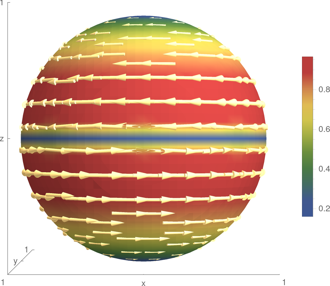
For , let and to be renormalized azimuthal and polar coordinates, respectively: . The corresponding directions are and . Consider the initial velocity field
| (7.1) | ||||
where is the distance from to the -axis. We take (for the velocity field is close to a rigid body rotation around the -axis), (perturbation parameter), and , , , (perturbation magnitudes and frequencies). Note that is tangential by construction, . The initial velocity field is illustrated in Figure 1.
Compared to the surface Stokes problem (2.2), the surface Navier–Stokes equations considered in this experiment are time-dependent and include inertia terms:
| (7.2) | ||||
where is the material derivative. For the unit sphere and initial condition such that , we have a Reynolds number . In our numerical tests we set , resulting in .
We note that equations (7.2) follows by tangential projection of a fluid system governing the evolution of a viscous material layer under the assumption of vanishing radial motions; see [20]. The operator can be seen as covariant material derivative. One checks the identity for a tangential vector field , which we further use in the finite element formulation.
We outline the discretization approach used for the simulation of this surface Navier–Stokes problem. The trace – Taylor–Hood finite element method as described in this paper, cf. (FEM), is applied for the spatial discretization. Discretization parameters were chosen as , , and , cf. (4.2). We use the BDF2 scheme to approximate and linearize the inertia term at as , where is the linear extrapolation of velocity fields from two previous time nodes, and . The grad-div stabilization term [28], with , is added to the finite element formulation to better enforce divergence free condition. This stabilization also facilitates the construction of preconditioners for the resulting algebraic systems [19]. No further stabilizing terms, e.g., of streamline diffusion type, were included in the method, since the computed solution does not reveal any spurious modes.
The method is implemented in the DROPS package [10]. For this series of experiments, an initial triangulation was build by dividing into cubes and further splitting each cube into 6 tetrahedra with . Further, the mesh is refined only close to the surface, and denotes the level of refinement so that .

We perform numerical simulations for mesh levels . The DROPS package currently does not support parametric elements, so for a sufficiently accurate numerical integration we use a piecewise linear approximation of with levels of local refinement, where , , ; see section 6.3 in [33] for further details. The time interval is fixed to be . We use uniform time stepping with , and for mesh levels and , respectively.
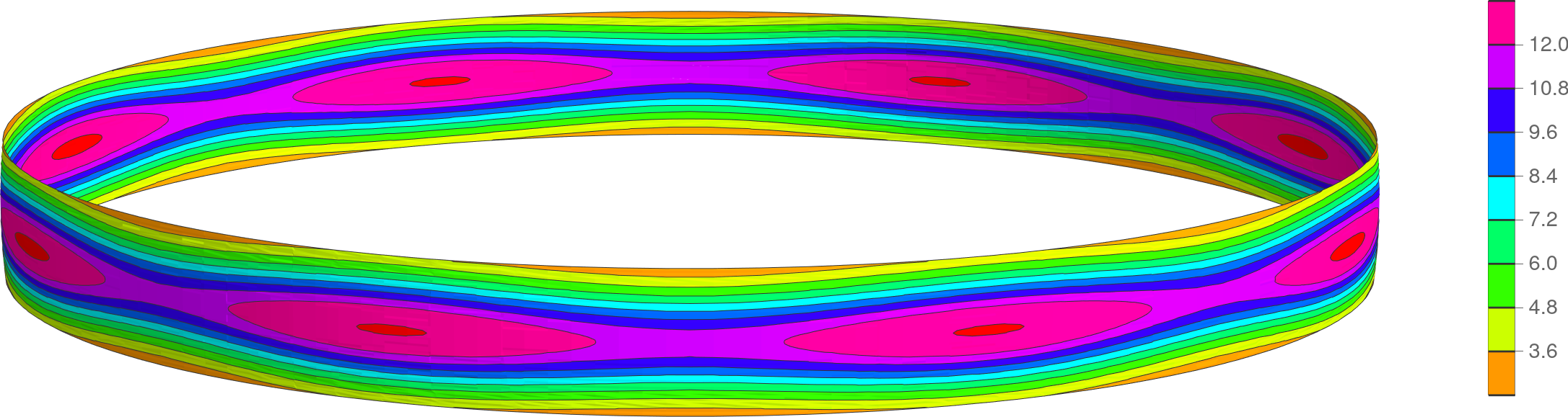
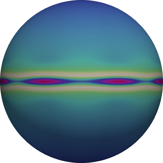
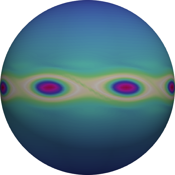
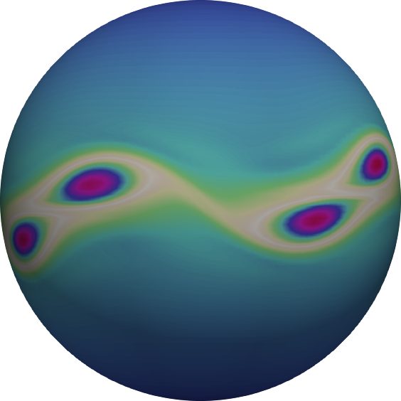
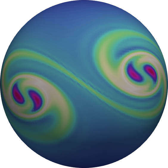
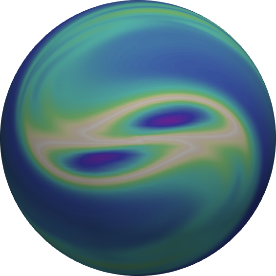
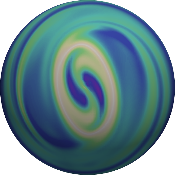
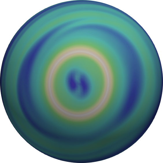
Figure 2 shows several snapshots of the surface vorticity, , computed on the finest mesh level 6. The trace – finite element method that we use reproduces qualitatively correct flow dynamics that follows the well known pattern of the planar Kelvin–Helmholtz instability development: we see the initial vortices formation in the layer followed by pairing and self-organization into two large counter-rotating vortices. Conservation of the initial zero angular momentum prevents further pairing. The two remaining vortices should decay for due to energy dissipation.
We next assess the method by monitoring the energy dissipation of the computed solutions on three subsequent levels. To have a better insight into the expected behaviour, we note that the initial velocity is -orthogonal to all rigid tangential motions of , functions from . It is straightforward to check that a velocity field that solving (7.2) preserves this orthogonality condition for all and hence it satisfies the following Korn inequality:
| (7.3) |
For the total kinetic energy , testing (7.2) with and applying (7.3) leads to the following identity and a corresponding energy bound:
We outline an approach for estimating the Korn constant . The best value of this constant is obtained if is the smallest strictly positive eigenvalue of the diffusion operator restricted to the space of tangential divergence free vector fields, cf. (7.3). We have the following relation between this surface diffusion operator and the Hodge-de Rham operator (see, eq. (3.18) in [20]):
| (7.4) |
where is the Gauss curvature ( for ). The eigenvalues of for the unit sphere are given by , , [8, p.349]. The tangential rigid motions are eigenfunctions corresponding to . Hence, we estimate:
resulting in 111Results of numerical experiments (not included), strongly suggest that for .. Substituting this in the above estimate for the kinetic energy, we arrive at the bound
| (7.5) |
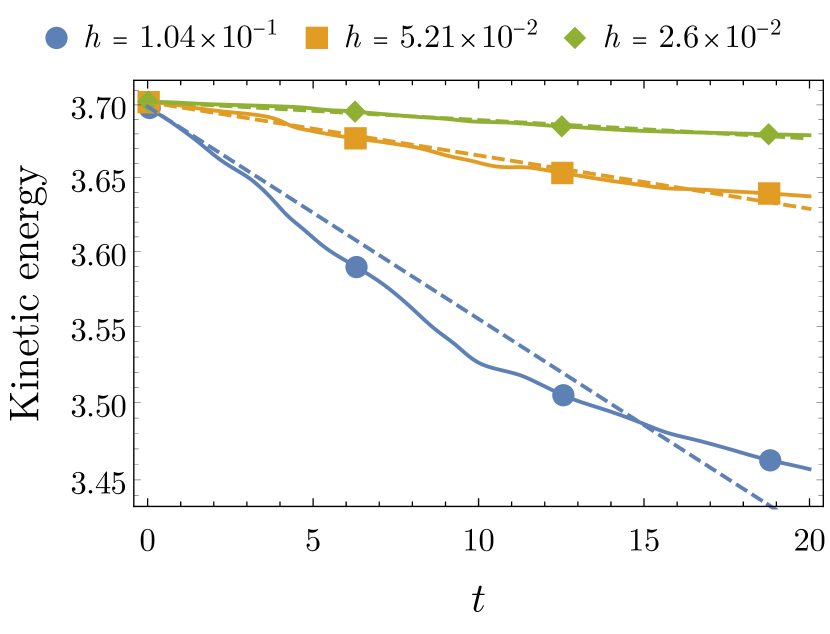
In Figure 3 we show the kinetic energy plots for the computed solutions together with exponential fitting. There are two obvious reasons for the computed energy to decay faster than the upper estimate (7.5) suggests: the presence of numerical diffusion and the persistence of higher harmonics in the true solution. On the finest mesh the numerical solution looses about of kinetic energy up to the point when the solution is dominated by two counter-rotating vortices. This compares well to results computed with a higher order method in [41] for the planar case with .
Acknowledgment
The authors Th. Jankuhn and A. Reusken wish to thank the German Research Foundation (DFG) for financial support within the Research Unit “Vector- and tensor valued surface PDEs” (FOR 3013) with project no. RE 1461/11-1. M.O. and A.Zh. were partially supported by NSF through the Division of Mathematical Sciences grant 1717516.
References
- [1] Netgen/NGSolve. https://ngsolve.org/.
- [2] SciPy. https://www.scipy.org/.
- [3] M. Arroyo and A. DeSimone, Relaxation dynamics of fluid membranes, Phys. Rev. E, 79 (2009), p. 031915.
- [4] A. Bonito, A. Demlow, and M. Licht, A divergence-conforming finite element method for the surface Stokes equation, Preprint arXiv:1908.11460, (2019).
- [5] P. Brandner and A. Reusken, Finite element error analysis of surface Stokes equations in stream function formulation, Preprint arXiv:1910.09221, (2019).
- [6] H. Brenner, Interfacial transport processes and rheology, Elsevier, 2013.
- [7] E. Burman, P. Hansbo, M. G. Larson, and A. Massing, Cut finite element methods for partial differential equations on embedded manifolds of arbitrary codimensions, ESAIM: Mathematical Modelling and Numerical Analysis, 52 (2018), pp. 2247–2282.
- [8] B. Chow, S.-C. Chu, D. Glickenstein, C. Guenther, J. Isenberg, T. Ivey, D. Knopf, P. Lu, F. Luo, and L. Ni, The Ricci flow: techniques and applications. Part IV: Long-time solutions and related topics, American Mathematical Society, 2007.
- [9] A. Demlow and G. Dziuk, An adaptive finite element method for the Laplace-Beltrami operator on implicitly defined surfaces, SIAM J. Numer. Anal., 45 (2007), pp. 421–442.
-
[10]
DROPS package.
http://www.igpm.rwth-aachen.de/DROPS/. - [11] G. Dziuk, Finite elements for the Beltrami operator on arbitrary surfaces, in Partial differential equations and calculus of variations, S. Hildebrandt and R. Leis, eds., vol. 1357 of Lecture Notes in Mathematics, Springer, 1988, pp. 142–155.
- [12] T.-P. Fries, Higher-order surface FEM for incompressible Navier-Stokes flows on manifolds, International Journal for Numerical Methods in Fluids, 88 (2018), pp. 55–78.
- [13] G. G. Fuller and J. Vermant, Complex fluid-fluid interfaces: rheology and structure, Annual review of chemical and biomolecular engineering, 3 (2012), pp. 519–543.
- [14] J. Grande, C. Lehrenfeld, and A. Reusken, Analysis of a high-order trace finite element method for PDEs on level set surfaces, SIAM Journal on Numerical Analysis, 56 (2018), pp. 228–255.
- [15] B. Gross, N. Trask, P. Kuberry, and P. Atzberger, Meshfree methods on manifolds for hydrodynamic flows on curved surfaces: A generalized moving least-squares (gmls) approach, Preprint arXiv:1905.10469, (2019).
- [16] M. E. Gurtin and A. I. Murdoch, A continuum theory of elastic material surfaces, Archive for Rational Mechanics and Analysis, 57 (1975), pp. 291–323.
- [17] A. Hansbo and P. Hansbo, An unfitted finite element method, based on Nitsche’s method, for elliptic interface problems, Comput. Methods Appl. Mech. Engrg., 191 (2002), pp. 5537–5552.
- [18] P. Hansbo, M. G. Larson, and K. Larsson, Analysis of finite element methods for vector Laplacians on surfaces, IMA J. Numer. Anal., (2019).
- [19] T. Heister and G. Rapin, Efficient augmented Lagrangian-type preconditioning for the Oseen problem using Grad-Div stabilization, International Journal for Numerical Methods in Fluids, 71 (2013), pp. 118–134.
- [20] T. Jankuhn, M. A. Olshanskii, and A. Reusken, Incompressible fluid problems on embedded surfaces: Modeling and variational formulations, Interfaces and Free Boundaries, 20 (2018), pp. 353–377.
- [21] T. Jankuhn and A. Reusken, Higher order trace finite element methods for the surface Stokes equation, Preprint arXiv:1909.08327, (2019).
- [22] , Trace finite element methods for surface vector-Laplace equations, Preprint arXiv:1904.12494. Accepted for publication in IMA J. Numer. Anal., (2019).
- [23] P. L. Lederer, C. Lehrenfeld, and J. Schöberl, Divergence-free tangential finite element methods for incompressible flows on surfaces, Preprint arXiv:1909.06229, (2019).
- [24] C. Lehrenfeld, High order unfitted finite element methods on level set domains using isoparametric mappings, Computer Methods in Applied Mechanics and Engineering, 300 (2016), pp. 716–733.
- [25] C. Lehrenfeld and A. Reusken, Analysis of a high-order unfitted finite element method for elliptic interface problems, IMA J. of Numer. Anal., 38 (2017), pp. 1351–1387.
- [26] I. Nitschke, S. Reuther, and A. Voigt, Hydrodynamic interactions in polar liquid crystals on evolving surfaces, Physical Review Fluids, 4 (2019), p. 044002.
- [27] I. Nitschke, A. Voigt, and J. Wensch, A finite element approach to incompressible two-phase flow on manifolds, Journal of Fluid Mechanics, 708 (2012), pp. 418–438.
- [28] M. Olshanskii and A. Reusken, Grad-div stablilization for Stokes equations, Mathematics of Computation, 73 (2004), pp. 1699–1718.
- [29] M. Olshanskii, A. Reusken, and X.Xu, A stabilized finite element method for advection-diffusion equations on surfaces, IMA J Numer. Anal., 34 (2014), pp. 732–758.
- [30] M. A. Olshanskii, A. Quaini, A. Reusken, and V. Yushutin, A finite element method for the surface Stokes problem, SIAM Journal on Scientific Computing, 40 (2018), pp. A2492–A2518.
- [31] M. A. Olshanskii and A. Reusken, Trace finite element methods for PDEs on surfaces, in Geometrically Unfitted Finite Element Methods and Applications, S. P. A. Bordas, E. Burman, M. G. Larson, and M. A. Olshanskii, eds., Cham, 2017, Springer International Publishing, pp. 211–258.
- [32] M. A. Olshanskii, A. Reusken, and J. Grande, A finite element method for elliptic equations on surfaces, SIAM J. Numer. Anal., 47 (2009), pp. 3339–3358.
- [33] M. A. Olshanskii, A. Reusken, and A. Zhiliakov, Inf-sup stability of the trace - Taylor–Hood elements for surface PDEs, Preprint arXiv:1909.02990, (2019).
- [34] M. A. Olshanskii and V. Yushutin, A penalty finite element method for a fluid system posed on embedded surface, Journal of Mathematical Fluid Mechanics, 21 (2019), p. 14.
- [35] M. Rahimi, A. DeSimone, and M. Arroyo, Curved fluid membranes behave laterally as effective viscoelastic media, Soft Matter, 9 (2013), pp. 11033–11045.
- [36] P. Rangamani, A. Agrawal, K. K. Mandadapu, G. Oster, and D. J. Steigmann, Interaction between surface shape and intra-surface viscous flow on lipid membranes, Biomechanics and modeling in mechanobiology, (2013), pp. 1–13.
- [37] A. Reusken, Analysis of trace finite element methods for surface partial differential equations, IMA J. Numer. Anal., 35 (2015), pp. 1568–1590.
- [38] , Stream function formulation of surface Stokes equations, IMA J. Numer. Anal., (2018).
- [39] S. Reuther and A. Voigt, Solving the incompressible surface Navier-Stokes equation by surface finite elements, Physics of Fluids, 30 (2018), p. 012107.
- [40] A. Sahu, Y. Omar, R. Sauer, and K. Mandadapu, Arbitrary Lagrangian–Eulerian finite element method for curved and deforming surfaces, J. Comp. Phys., 407:109253 (2020).
- [41] P. W. Schroeder, V. John, P. L. Lederer, C. Lehrenfeld, G. Lube, and J. Schöberl, On reference solutions and the sensitivity of the 2D Kelvin–Helmholtz instability problem, Computers & Mathematics with Applications, 77 (2019), pp. 1010–1028.
- [42] L. Scriven, Dynamics of a fluid interface equation of motion for Newtonian surface fluids, Chemical Engineering Science, 12 (1960), pp. 98–108.
- [43] J. C. Slattery, L. Sagis, and E.-S. Oh, Interfacial transport phenomena, Springer Science & Business Media, 2007.
- [44] A. Torres-Sánchez, D. Millán, and M. Arroyo, Modelling fluid deformable surfaces with an emphasis on biological interfaces, Journal of Fluid Mechanics, 872 (2019), pp. 218–271.
- [45] A. Torres-Sanchez, D. Santos-Olivan, and M. Arroyo, Approximation of tensor fields on surfaces of arbitrary topology based on local Monge parametrizations, arXiv:1904.06390, (2019).