Bayesian item response models for citizen science ecological data.

Abstract

1. So-called “citizen science” data elicited from crowds has become increasingly popular in many fields including ecology. However, the quality of this information is being frequently debated by many within the scientific community. Modern citizen science implementations therefore require measures of the users’ proficiency that account for the difficulty of the tasks.

2. We introduce a new methodological framework of item response and linear logistic test models with application to citizen science data used in ecological research. This approach accommodates spatial autocorrelation within the item difficulties, and produces relevant ecological measures of species and site-related difficulties, discriminatory power and guessing behaviour. These, along with estimates of the subjects’ abilities, allow better management of these programs and provide deeper insights. This paper also highlights the fit of item response models to big data via divide-and-conquer.

3. We found that the suggested methods outperform the traditional item response models in terms of RMSE, accuracy, and WAIC based on leave-one-out cross-validation on simulated and empirical data.

4. We present a comprehensive implementation using a case study of species identification in the Serengeti, Tanzania. The R and Stan codes are provided for full reproducibility. Multiple statistical illustrations and visualisations are given which allow extrapolation to a wide range of citizen science ecological problems.

1 Introduction

Citizen science is becoming extremely valuable in modern science helping to overcome some of the limitations in conventional science settings [79, 40, 11]. For example, large worldwide networks of participants are contributing to conservation efforts, generating large volumes of valuable information and achieving a better understanding and awareness of biodiversity [60]. The numerous examples found in the literature range from the worldwide estimation of the abundance of birds [88], to species of mammals in Africa [89], the distribution of jaguars in the Peruvian Amazon [61] and hard coral cover estimation in the Great Barrier Reef [73]. Plenty of projects can be found in online platforms e.g. iNaturalist, eButterfly, Zooniverse.

However, the quality of the data produced by volunteers is often questioned in the scientific community [11, 50]. Contributors’ commitment, abilities, training and effort along with the difficulty of the task affect their performance [48, 25]. In crowdsourcing projects, there is a growing interest in assessing how well users can perform estimation and classification tasks and specifically in measuring their latent abilities [e.g. 28].

This can be approached using Item Response Theory (IRT) models, which are special cases of the family of generalized mixed models and consist of the estimation of the latent participant’s performance while accounting for the task’s difficulty. There is an extensive literature on the use of IRT in multiple fields ranging from psychology, political and social sciences [34, 52, 59], and education to statistics and computer sciences [96, 24, 55, 62].

Multiple frequentist and Bayesian approaches to IRT have been employed, along with a wide range of computational methods. For example, for classification tasks, common models found in the literature are the logistic and normal models, while graded response models are employed for ordered categorical variables. Several implementations of Bayesian IRT models using different statistical languages have been also published. For instance, Curtis et al. [21] used BUGS/JAGS, Grant et al. [37], Luo and Jiao [57] and Bürkner [12] used Stan while Stone and Zhu [87] employed SAS. Multiple examples can be found in Fox [31] and in the Stan user manual [17].

Latent variable models that have been used in ecology to describe the occurrence of species as a function of latent predictors [74, 94] are related to the IRT models. The use, however, different formulations. However, not much attention has been paid to estimating the abilities and performance measures for citizen science in ecological settings.

Measures of participants’ abilities and their differentiation are relevant for several reasons. Statistical inference from crowdsourced data assigns greater weights to information from more competent users [51, 8, 45]. In the absence of a gold standard, ability-derived weights can be used in consensus voting algorithms or for building reputation and leaderboard systems [84, 15]. Extremely low abilities are generally associated with careless, non-genuine respondents and bots which are generally excluded for being non-informative and representing a burden for inference and computation.

In this research, subjects are referred to as participants, citizens, annotators, users, while items refer to information sources (images, videos, audio files, etc.) [102, 38, 78]. However, we concentrate on the particular case species identification on images.

Data collected in citizen science projects is challenging compared to what is found in the traditional item response literature. For example, the number of items for classifications can be large, reaching often hundreds of thousands and in some cases, it could be larger than the number of users. Additionally, participants score a different number of items. Some users engage heavily while others contribute lightly [41]. However, a user rarely scores all the items if the number is large. As a consequence, generally, a large proportion of data is missing. Overall, the skills of the respondents are generally heterogeneous, ranging from experts to beginners.

These complications are exacerbated when the focus of citizen science is on the classification of features or the identification of species in images. In this setup, camera, site, and species-specific factors can affect the underlying item difficulty level [99]. Several image specific components maybe also critical e.g.: the camera resolution, brand, flash effect, etc. Other crucial factors are the visibility, time of the day (day or night), landscape and the vegetation. It has been also well documented that some species are far more difficult to identify than others. Look-alike or closely related species are more challenging, leading frequently to misclassifications [19, 41].

In ecological research, items such as images are usually georeferenced [60, 15]. An added complication in such a setting is that items that are geographically close to each other tend to have more similar characteristics such as the probability of containing the target species, compared to those that are further away. For this reason, many citizen science applications account for spatial autocorrelation. Some examples can be found in Pagel et al. [69], Purse et al. [75], Arab and Courter [4], Humphreys et al. [44], Altwegg and Nichols [3]. Latent image difficulties tend to exhibit spatial auto-correlation, which should be accounted for in the IRT models. Ignoring such autocorrelation can lead to biased parameter estimates and underestimating the associated standard errors and hence potentially erroneous inference. See e.g. Lichstein et al. [53], Ver Hoef et al. [91].

The identification of areas with spatial correlation is also relevant for survey administration purposes. Distinguishing areas in which the items have relatively high difficulties is vital to provide recommendations on how to improve the quality of the images, generate more useful training and users’ documentation, and to better manage the order in which tasks are presented for classification, etc. Images from camera traps difficult to identify might indicate technical issues. Additionally, identification of images with no visible species and covered by vegetation is relevant for data cleaning purposes.

A brief literature review of IRT models

Since the introduction of the Rasch model [77], several extensions and variations have been proposed for the IRT. The three parameter logistic model (3PL) [9] and the graded response model by [80] are among the most relevant contributions. Many examples and implementations can be found in widely known published textbooks e.g. Baker and Kim [6], van der Linden and Hambleton [54], Embretson and Reise [27], De Ayala [23]. IRT modelling has been approached from the generalized linear model (GLM) perspective and a very didactic discussion can be found in Wilson et al. [100]. In a spatial context, Cançado et al. [16] has suggested a model that borrows some principles of spatial statistics for the identification of spatial clusters. Another model accounting for changes in space and time is presented in Juhl [46].

A new class of state-space model called dynamic item response is introduced by Wang et al. [93] for longitudinal data. Under the principle that the abilities change over time, this dynamic approach produces a growth curve for the latent trait. Another dynamic IRT model was presented by Weng et al. [97], where model parameters are updated as the data becomes available in a sequential manner.

Within the Bayesian philosophy, multiple model implementations have been suggested e.g. Patz and Junker [70], Fox [31], Albert [1]. Possibly the greatest limitation of Bayesian item response models is the identifiability issues arising from having a large number of parameters to be estimated from the data. For a detailed discussion on identifiability see e.g. Fox [31]. Strategies like anchoring the sum or the mean of the difficulties to zero have been suggested to cope with this limitation.

In this research, we introduce extensions of the 3PL item response model (U)sing (S)patially dependent item difficulties (henceforth 3PLUS) and variations of the linear logistic test model (LLTM). These approaches are tailored to citizen science data elicited from georeferenced images. We discuss the advantages and limitations of the suggested methods. We take a Bayesian approach for modelling using prior information for the parameters of interest. This has multiple advantages which includes better parameter estimates for cases when the number of samples for some users is relatively small [64, 20]. We start with a simulation study to compare the proposed model to the state of the art. This is followed by a case study of citizen science image classification in the Serengeti, Africa.

2 Methods

In the case of citizen-elicited classification in an image, a common approach is to select points and ask the user whether each point contains the target class or species. Let the binary response variable $Y$ represents whether the question was correctly answered by the $i^{\textrm{th}}$ citizen ($i=1,\cdots,I$), in the $j^{\textrm{th}}$ image ($j=1,\cdots,J$) for the $k^{\textrm{th}}$ point ($k=1,\cdots,K$), $Y_{ijk}\sim\textrm{Bern}\left(p_{ijk}\right)$.

In some cases the interest is on identifying species in the whole image and the above case is reduced to $k=1$. The probability $p_{ijk}$ of a correct answer can be modeled using the three-parameter logistic model [56, 6].

$$p_{ijk}=\eta_{j}+\left(1-\eta_{j}\right)\frac{1}{1+\textrm{exp}\left\{-\alpha_{j}\left(\theta_{i}-b_{j}\right)\right\}}.$$ (1)

Here $\theta_{i}$ is the latent ability of the $i^{\textrm{th}}$ user, such that the higher the $\theta_{i}$ values are, the larger the probability of identifying correctly the class of the item. The parameter $b_{j}$ represents the difficulty of the $j^{\textrm{th}}$ image and $\alpha_{j}>0$ represents the slope or discrimination parameter of image $j$ indicating how quickly the function will go from 0 to 1. The parameter $\eta_{j}$ is the pseudoguessing parameter of the $j^{\textrm{th}}$ image that is the lower asymptote, which accounts for users’ chance of answering correctly by guessing.

Several variations of this model can be found in the literature [6, 23]. For example, the two-parameter logistic (2PL) model is a reduction arising from setting $\eta_{j}=0$, while the Rasch model is obtained using $\eta_{j}=0$ and $\alpha_{j}=1$ [13]. Another popular approach replaces the logistic link function by the probit link [2]. The difficulty, slope and pseudoguessing parameter are considered locally homogenous within the image, so, the parameters $b_{j}$, $\alpha_{j}$ and $\eta_{j}$ are common for each point $k$. The effect of these parameters on $p_{ijk}$ is shown in Fig.1.

Figure 1: Item characteristic curves of the 3PL model giving the probability of correctly answering a standard item ($b=0$) as a function of the latent user ability $\theta$. In (a) we compare curves from three different values of the slope $\alpha$ with no guessing i.e. $\eta=0$. In (b) we compare curves using three pseudoguessing values $\eta=0,0.1,0.2$ and a fixed value of $\alpha=1$.

In this paper, we suggest a spatial extension of the 3PL model in which we model the difficulties as a random spatial effect. We adopt a conditional autoregressive (CAR) prior [7], noting that the general approach can accommodate other representations of the spatial autocorrelation. CAR priors have been found to adequately capture spatial variability in citizen science applications [69, 75, 5, 4, 3]. However, multiple other alternatives such as Gaussian random fields [44] and stochastic partial differential equations (SPDE) [72] can be found in the literature. Under the CAR prior, the distribution of $b$ conditional on the first-order neighbours is the average of the $n_{l}$ first-order neighbours plus Gaussian noise.

$$b_{l}|b_{m},\tau_{b}\sim\mathcal{N}\left(\frac{1}{n_{l}}\sum_{l\sim m}^{.}b_{m},\frac{1}{\tau_{b}n_{l}}\right)$$ (2)

where $n_{l}$ is the number of neighbours for region $l$, $l\sim m$ means $l$ and $m$ are neighbours and $l\neq m$. The parameter $\tau_{b}$ is the precision of the spatial effect.

2.1 LLTM model extensions

We propose a further extension of the 3PLUS model called item explanatory, which is a special case of the linear logistic test model (LLTM) [30, 100]. In this approach, the item parameter ($b_{j}$) is a linear combination of factors governing the difficulty ($\sum_{m=1}^{M}\beta_{m}X_{jm}$), where $M$ is the number of factors. This model does not give directly an indication of the difficulties associated with the images, but explains the effect of the item related factors. For instance, often we are interested in the camera difficulty that accounts for the image quality and on the complications associated with the site (unique latitude and longitude) in which the camera is placed rather than on the individual image difficulties.

Similarly, the intrinsic difficulty associated with the species can be considered. This explains the misclassification error due to species that look like the target one (e.g. Grant’s vs Thomson’s gazelle) and also mimic animal-specific behavior and features.

The probability that citizen $i$ correctly identifies species $l$ in the $j^{\textrm{th}}$ site is given by:

$$p_{ijl}=\eta_{.}+\left(1-\eta_{.}\right)\frac{1}{1+\textrm{exp}\left\{-\alpha_{.}\left(\theta_{i}-\beta_{j}I_{j}-\beta_{l}I_{l}\right)\right\}}$$ (3)

where $I_{j}$ and $I_{l}$ are indicator variables of the site and species respectively. The parameters $\beta_{j}$ and $\beta_{l}$ are difficulties associated with the site and species respectively. The pseudoguessing $\eta_{.}$ can be associated with the species or with the sites. That is why we indexed it with a dot (.). The first case is more reasonable since it explains what species are more likely to be correctly classified due to guessing. High values of species-related pseudoguessing values indicate species that are easily classified for those users with less proficiency. Similarly, species or site-specific discrimination parameters can be estimated in the model ($\alpha_{l}$ or $\alpha_{j}$), showing which items are more suitable for differentiating the users.

To avoid confusion, we will retain the notation previously used to refer to the models but we add a prime symbol (’) to denote test model extensions. That is, the test model (3PLUS’) of Eq.3 is an extension of the model introduced in Eq.1 with $b_{j}$ replaced by $\beta_{j}I_{j}+\beta_{l}I_{l}$.

3 Simulation study

We first present a simulation study to compare the performance of the 3PL and 3PLUS models. Consider $j=225$ unique geographical locations in a 15 $\times$ 15 grid, which is generally large enough for the illustration and has been employed in several practical designs e.g. [89]. For the image difficulties we generated the spatial autocorrelation using a multivariate normal distribution, $b_{j}\sim\textrm{MVN},\left(\mu_{b}=0,\Sigma_{b}\right)$, with a spatial covariance matrix $\Sigma_{b}$ obtained using the simple exponential form e.g.: $\Sigma_{b}=\exp(-d/r)$, where $d$ is the Euclidean distance between locations and $r$ is a scaling parameter.

Fig.S.12 shows Voronoi polygons using the image locations as centroids and boundaries based on Euclidean distance [68, 36], which were used to define the spatial domain in the model. In (a) we show the spatial association between the difficulties and regions characterized by clusters of images that are easy (light blue) and hard (dark blue) to classify. Consider five groups of users with fixed abilities: $\theta_{.}=\left\{-1,-0.5,0,0.5,1\right\}$. We set several values for the discrimination ($\alpha$) ranging from small to large slopes, $\alpha_{.}=\left\{0.25,0.50,\cdots,1.50,1.75\right\}$. We assume having six target classes and consider that users will have on average 1 in 6 chances of guessing the true target class with extremely low knowledge. Therefore, a pseudoguessing parameter $\eta\sim\textrm{Beta}\left(1,5\right)$ is employed, which is a weakly informative prior commonly used in the literature for this parameter.

A random user, slope and pseudoguessing value is assigned with replacement to each image id. Each citizen scores multiple images and each image is classified several times. Every image contains 15 elicitation points. Using $p$ from Eq.1 we simulated binary realizations using the Bernoulli distribution.

3.1 Fitting the Bayesian models

We want to learn about the latent parameters $\theta_{i}$, $b_{j}$, $\alpha_{j}$ and $\eta_{j}$ using the observed variable ($Y_{ijk}$). We employ Markov chain Monte Carlo simulations, in particular Hamiltonian Monte Carlo (HMC), in the software package Stan [17] which is based on the no-U-turn sampler (NUTS) [39]. We used 3 chains each of 50,000 samples after we discarded a burn-in of 20,000 samples. We used the prior distributions shown in Fig 2. The CAR prior was implemented according to Morris et al. [65].

$$\theta_{i} \sim\mathcal{N}\left(0,\sigma_{\theta}\right)$$ # hierarchical informative prior on the abilities

$$\sigma_{\theta} \sim\textrm{uniform}\left(0,10\right)$$ # flat prior for the user’s abilities sd

$$b_{3PL} \sim\mathcal{N}\left(\mu_{b},\sigma_{b}\right)$$ # informative prior on the difficulties in 3PL model

$$\mu_{b} \sim\mathcal{N}\left(0,5\right)$$ # normal prior for the mean of the item difficulty

$$\sigma_{b} \sim\textrm{Cauchy}\left(0,5\right)T(0,)$$ # flat prior for the sd of the item difficulty

$$b_{\textrm{3PLUS}} \sim\textrm{CAR}\left(\tau,W,D\right)$$ # CAR prior for the spatial model

$$\tau_{b} \sim\textrm{Gamma}\left(1,1\right)$$ # precision of the spatial effect

$$\alpha \sim\mathcal{N}\left(1,\sigma_{\alpha}\right)$$ # normal prior with mean 1 on the slope

$$\sigma_{\alpha} \sim\textrm{Cauchy}\left(0,5\right)T(0,) T(0,)$$ # half Cauchy prior for the slope sd, where means lower truncation at 0

$$\eta \sim\textrm{beta}\left(1,5\right)$$ # weakly informative prior on the pseudoguessing

$$\tau$$ # precision parameter in the CAR prior

$$D$$ _m×m # diagonal matrix

$$W$$ _m×m # adjacency matrix

Figure 2: Prior distributions used in the models.

The parameter $b_{3PL}$ is the difficulty in the traditional model (3PL), while $b_{\textrm{3PLUS}}$ represents the difficulty in the spatial approach. We anchored the ability of the “reference” user by setting it equal to zero. This was done by fitting the model in the mirt package [18] and finding the user with the score closest to zero.

The comparison of the models was based on the following criteria: (1) confusion matrix and the accuracy when estimating the parameters (difficulties, abilities, slopes, pseudoguessing), (2) Root Mean Square Error (RMSE), (3) Watanabe–Akaike information criterion (WAIC) [95].

3.2 Simulation results

Both models produced similar user abilities estimates (See Fig 11(a) and 11(b) in the Supplementary Material). The RMSE for the 3PLUS model was slightly smaller (0.2036 vs 0.2092). The 3PLUS model produces better difficulty estimates (Fig 3(a) and S.12 ) with a better accuracy and precision. The yellow labels in Fig S.12 (b) and (c) are the locations where the true difficulties estimates were not correctly identified. The 3PLUS model achieved an 80% prediction accuracy of the difficulty classes compared to 62.22% under the 3PL model. This model also halved the RMSE: $\textrm{RMSE}_{\textrm{3PLUS}}=$ 0.2596 vs. $\textrm{RMSE}_{\textrm{3PL}}=0.4808$. The correlations between the estimated difficulties and the true values were $r^{2}_{\textrm{3PLUS}}=0.9685$ vs $r^{2}_{\textrm{3PL}}=0.8776$. Both models produced similar estimates of the slope ($\alpha$), but the pseudoguessing parameter ($\eta$) was better estimated in the 3PLUS model in terms of RMSE. See Fig 3(b) and 3(c). The 3PLUS model also produces a slightly smaller WAIC (44,586.7 vs 44,637.0) and LOO (leave-one-out cross-validation) values (44,588.1 vs 44,638.7).

(a) Boxplot of the difficulties

(b) Slope

(c) Guessing

Figure 3: (a) Boxplot of the estimated difficulties for locations 51-100. The true parameter value (red dots) in the traditional 3PL (left) and the 3PLUS model (right).Estimated slope (b) and guessing (c) parameters in the traditional 3PL (green) and the 3PLUS model (blue). The y-axis gives the estimates while the x-axis represents the true value. The ideal case of perfect estimation is represented in black color.

3.3 Effect of having more classifications

One of the main strengths of citizen science programs is the rapid acquisition of a large volume of classifications [10]. However, several issues relevant to these programs are not often quantified. For instance, how does the number of participants affect the precision of the estimates? How many sampled locations are needed? What is a suitable number of classifications per image? We designed an experiment to assess the effects of these three factors on the model fit and considered the following values:

1. grid size: This represents the number of unique geo-tagged locations for the items, e.g. image GPS coordinates: 10$\times$10, 15$\times$15 and 25$\times$25.

2. number of participants: 9, 21 and 60. This was chosen to be very small, small and medium based on the impact or the precision of the estimates.

3. the number of elicitation points per image: This frequently arises in approaches used in ecology and is also known as the random point count methodology [e.g. 49] : 5, 15 and 25.

For this combination of parameters, we generated 27 datasets and fit both the 3PL and the 3PLUS models. Fig 4 depicts a comparison between the two models based on (a) RMSE of the difficulties and (b) the accuracy of retrieving the true category. The three grid sizes are represented with different line types. The panels show the number of users. The proposed model produces a substantially smaller RMSE and better accuracy for most of the factor combinations. The greater the number of elicitations and users the smaller the RMSE and the larger the accuracy is in both models.

We fitted Bayesian regression models for the parameters (difficulties, abilities, slopes, and pseudoguessing) to the (log) RMSE as a function of the factors plus the model type using as a baseline factor the benchmark (3PL). The posterior density and trace-plots showed well-mixed chains and convergence. In the model for the log RMSE of the difficulties (Table S.2), there are more differences between the models than when accounting for the factors. The numbers of elicitations, citizens and the grid size were found to affect the RMSE. We found similar outcomes for the models using as a response variable the RMSE in the abilities, slopes, and pseudoguessing. A negative value in the model dummy variable means that a reduced RMSE is obtained when using the 3PLUS model. Larger numbers of elicitations and citizens also decrease the RMSE.

Fig 4 compares the RMSE of the difficulties, abilities, slopes and pseudoguessing parameters and the accuracy retrieving the difficulties in both models. The 3PLUS model produces smaller RMSE and the difference tends to be proportional to the number of users and the grid size.

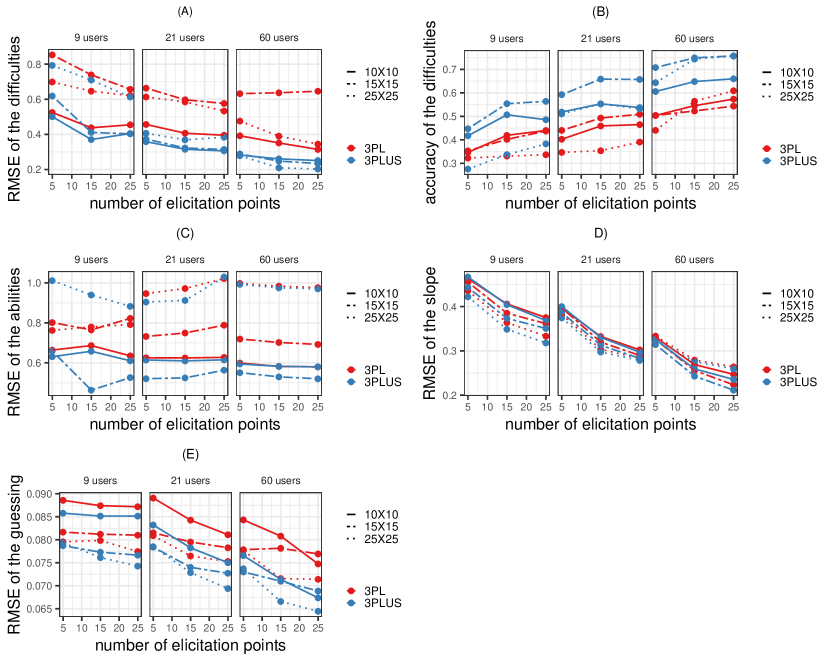
Figure 4: Root mean square error (RMSE) of the difficulties (A), abilities (C), slopes (D) and pseudoguessing (E) and difficulties accuracy (B) for each model (3PL vs 3PLUS). The x-axis represents the number of elicitation points/image and the panels give the number of users on each group. The grid size is plotted with different line types.

New algorithms are often computationally intensive and involve larger processing times. We performed the simulations on a High-Performance Computing (HPC) system with CPUs architecture Intel AVX and AVX-2. No substantial differences in computing times were found between models.

4 Hakuna my data: A case study of species identification in the Serengeti

4.1 The Serengeti data

Swanson et al. [89] describe a citizen science project that identified species from the Serengeti, Tanzania. This project is hosted on Zooniverse (https://www.zooniverse.org/projects/zooniverse/snapshot-serengeti) and captured more than a million images, with a total of 10.8 million classifications produced by 28,000 users. Images were obtained by camera traps in 225 spatial locations. The data contains image details of the classifications per user and includes the spatial component given by the location of the cameras. Swanson et al. [89] published several datasets including the original raw classification data, the consensus voting results and a gold standard dataset. The gold standard dataset included classifications by experts of 4,140 images. The proportion of correct classification per site showed spatial autocorrelation based on the Moran’s I test ($p<0.001$).

A total of 50 species categories were identified including wildebeest, zebra, buffalo, hartebeest, lion (female and male), etc. The categories impossible to identify and human were also included. The authors noted that subjects tend to use more the nothing here classification rather than guessing when they were not sure of the species. Two-dimensional kernel density plots of the three most abundant species (prey) plus female lion (predators) is shown in Fig 5.

Images were captured at different times of the day, including night time. Several other factors affecting the difficulty of the images are included: animal moving or feeding, the presence of babies, the relative position regarding the vegetation and camera placement, etc.

We selected the registered users with more than five classifications so that we can obtain suitable estimates of the abilities. For inclusion, images had to have a known location or site id. This produced a dataset composed of almost 5 million observations, from 21,347 citizens from 225 locations. The data and codes associated with the case study can be found in the repository https://github.com/EdgarSantos-Fernandez/staircase.

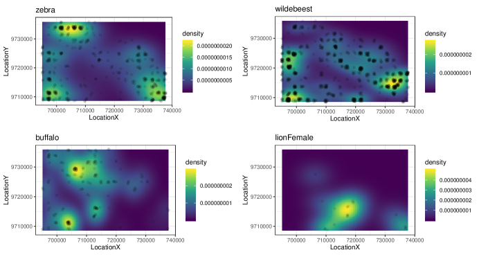
Figure 5: 2D kernel density plot of the three most abundant species (prey) in the gold standard dataset plus female lion (predators).

4.2 Analysis using the gold standard data and model comparison

Assessing the fit of several model variations and comparisons becomes difficult with large datasets. We first find the best performing model using the gold standard dataset and then fit it using the whole data. For simplicity, images with more than one species were excluded resulting in 88,517 observations.

We considered 10 model variations of Eq.3, shown in Table LABEL:tab:mods. We started with the 3PL and 3PLUS previously compared in the simulations. Eight linear logistic test models were studied, from a very simple (1PL’) to more complex (3PLUS’). Three variations of the 3PLUS’ are examined, resulting from permutations of the site and species slopes and pseudoguessings parameters. For instance, 3PLUS-2’ and 3PLUS-3’ involves a species-based guessing ($\eta_{l}$), while the slopes are site specific for 3PLUS-2’ ($\alpha_{j}$) and species dependent for 3PLUS-3’ ($\alpha_{l}$).

The 10 competing models were fit in Stan using four chains, 4000 iterations and a burn-in of 2000 reaching convergence. The estimates for the effective number of parameters $\hat{p}_{waic}$ were found to be unreliable, exceeding 0.4 [90], for which using leave-one-out cross-validation (LOO) is recommended. The LOO measure also seems appropriate since we are interested in the applicability to other users/items. See Table LABEL:tab:mods.

According to the LOO information criterion values, the 3PLUS-2’ model seems to be superior. In this model, the pseudoguessing parameter is species-related, while the slope is indexed to the site that accounts for the camera and location-specific factors.

Table 1: Model variations from the model in Eq.3 ($p_{ijl}=\eta_{.}+\left(1-\eta_{.}\right)\frac{1}{1+\textrm{exp}\left\{-\alpha_{.}\left(\theta_{i}-\beta_{j}I_{j}-\beta_{l}I_{l}\right)\right\}}$) where the citizen is indexed by $i$, the site location by $j$ and the species by $l$. The symbol ’ indicates test model extension.

Model	Name	Parameters	WAIC	LOO
3PL	traditional 3PL model	$\eta_{l}$, $\alpha_{l}$, $\theta_{i}$, $\beta_{l}$, $\beta_{j}=0$	94,396.2	94,443.9
3PLUS	spatial 3PL model	$\eta_{j}$, $\alpha_{j}$, $\theta_{i}$, $\beta_{j}\sim\textrm{CAR}(W,D,\tau)$ and $\beta_{l}=0$	86,153.3	86,205.8
1PL’	traditional 1PL test model	$\eta=0$, $\alpha=1$, $\theta_{i}$, $\beta_{l}$ and $\beta_{j}$	86,167.6	86,197.2
2PL’	traditional 2PL test model	$\eta=0$, $\alpha_{j}$, $\theta_{i}$, $\beta_{l}$ and $\beta_{j}$	85,401.2	85,453.6
3PL’	traditional 3PL test model	$\eta_{j}$, $\alpha_{j}$, $\theta_{i}$, $\beta_{l}$ and $\beta_{j}$	85,439.2	85,495.7
1PLUS’	spatial 1PL test model	$\eta=0$, $\alpha=1$, $\theta_{i}$, $\beta_{l}$ and $\beta_{j}\sim\textrm{CAR}(W,D,\tau)$	86,186.0	86,215.8
2PLUS’	spatial 2PL test model	$\eta=0$, $\alpha_{j}$, $\theta_{i}$, $\beta_{l}$ and $\beta_{j}\sim\textrm{CAR}(W,D,\tau)$	85,411.2	85,463.3
3PLUS-1’	spatial 3PL test model	$\eta_{j}$, $\alpha_{j}$, $\theta_{i}$, $\beta_{l}$ and $\beta_{j}\sim\textrm{CAR}(W,D,\tau)$	85,419.6	85,474.8
3PLUS-2’	spatial 3PL test model	$\eta_{l}$, $\alpha_{j}$, $\theta_{i}$, $\beta_{l}$ and $\beta_{j}\sim\textrm{CAR}(W,D,\tau)$	85,199.3	85,257.9
3PLUS-3’	spatial 3PL test model	$\eta_{l}$, $\alpha_{l}$, $\theta_{i}$, $\beta_{l}$ and $\beta_{j}\sim\textrm{CAR}(W,D,\tau)$	85,711.2	85,766.9

4.3 Item response modeling for big data

Fitting item response models to big datasets can be challenging and prohibitive within the Bayesian paradigm. Operations involving a large number of parameters often exceed the memory, processing and disk capacities, which is exacerbated if simulation-based computation/estimation such as MCMC is used. This is even more problematic when accounting for spatial autocorrelation [47, 22, 29].

In this section, we focus on modelling datasets too large to be fit directly in one machine or even on a modern HPC node. We use the dataset previously described, which is composed of almost 5 million classifications. The true answer (species) was obtained in the non-gold standard images using the majority vote.

We took a divide-and-conquer approach, also known as divide-and-recombine [83, 67, 92] splitting the big dataset into multiple shards or subsets. Models were fit to the independent subsets on independent machines with no communication, and subposterior estimates were then combined into global estimates using consensus Monte Carlo [83]. Specifically, we used weighted averages of the posterior MCMC chains, with weights inversely proportional to the variance of the posterior samples. At each iteration, the consensus estimate of a parameter is given by $\theta_{g}=\left(\sum_{s}^{S}W_{s}\right)^{-1}\sum_{s}^{S}W_{s}\theta_{sg}$, where $s$ is the subset or machine, $g$ is the iteration number, $\theta_{sg}$ is the estimate at the iteration $g$ from the machine $s$ and $W_{s}=\textrm{Var}\left(\theta|y_{s}\right)^{-1}$. The consensus Monte Carlo is known to produce an asymptotic approximation to the posterior based on the whole dataset [83]. However, multiple other options could have been explored to obtain the combined subposterior distributions [e.g. 67].

The number of observations of each location and species is large. However, the classifications per user varied from a few to several hundred. Thus, we employed stratified sampling with users as grouping criteria thereby splitting the dataset into 10 equal parts. This yielded 10 shards with approximately half a million observations per shard. Some users will not be represented on all the subsets, while most of the species and sites were estimated on every shard.

All the results from this section can be reproduced using the R Markdown file in the repository https://github.com/EdgarSantos-Fernandez/staircase, which illustrate (1) how to request resources on an HPC, (2) how to fit the models in Stan and (3) how to combine the posterior estimates.

Shards were fitted in parallel with no communication on a high performance computing (HPC) system using 10 CPUs, three processors and a request of 280 Gb of memory. Estimates of the latent parameters were obtained using the best performing model (3PLUS-2’) found in the previous section. We used three chains, a warm-up period of 3000 samples and 8000 iterations. It took approximately 42 hours to fit each model and to compute the WAIC. For combining the subposteriors into the whole dataset posterior, we modified the function consensusMCindep() from the R package parallelMCMCcombine [63]. This approach is suitable for normally distributed parameters (difficulties, abilities, slopes) and has been found to work satisfactorily also for non-normal variables [83] such as the pseudoguessing which is modelled using beta distributions. Summary statistics of some of the parameters of interest are shown in Table S.3.

On each machine, we obtained subposterior estimates for each of the parameters. For instance, in Fig 6 we show the estimates for nine users with good, moderate and poor classification skills (three on each group). In some cases, there could be a moderate variability on the estimates obtained from different shards e.g. user = 2. This is because by random, users will have a better performance in some subsets than in the others. See Fig S.13 for scatter plots comparing the posterior ability estimates in the 10 shards (abil1, abil2, etc.) and in the recombined consensus posterior (abil).

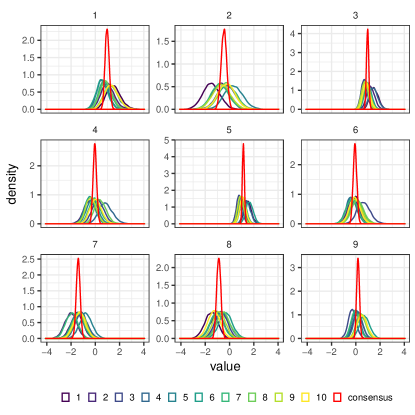
Figure 6: Posterior estimates of the abilities for nine users in 10 machines and the posterior obtained using the consensus approach (in red).

Fig 7 shows the user proficiency levels as a function of the proportion of correct classifications. Clustering the participants into groups based on their abilities is relevant for citizen science programs and crowdsourcing. For instance, the latent classifications are often obtained by majority or consensus vote. Weighted variations of the voting systems can be easily implemented using as weights the posterior abilities with some penalization based on the variability of these estimates. More effective compensation, rewards and bonuses can be readily implemented for example in projects using platforms such as Amazon Mechanical Turk. Finally, ability assessment is a powerful resource to detect software bots, careless participants, etc, which generally have the lowest ability scores (beginner group in Fig 7).

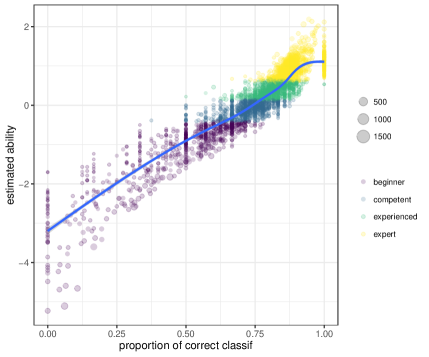
Figure 7: Posterior estimates of the users’ abilities vs their proportion of correct classifications. The size of the dots represents the users’ number of classifications.

Similarly, we obtained posterior distributions for the difficulties in identifying the species (Fig 8(a)). Species with mean positive values are more difficult to identify e.g. hyena striped. Other categories with negative estimates such as giraffe and zebra had a high probability of correct classification. Fig 8(b) shows the posterior estimates of the species difficulties as a function of the proportion of correct classification. On average citizens misclassified images containing humans with probability 0.10 and this could be considered as an indicator of careless responses.

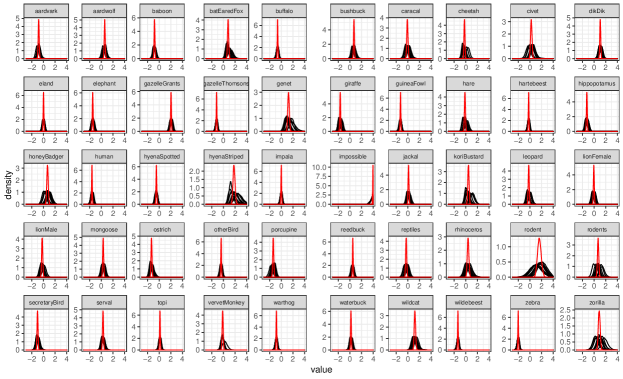
(a) Subposterior estimates of the species difficulties

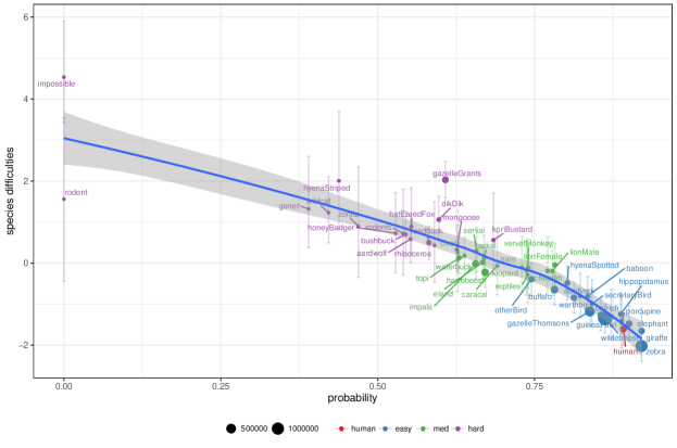
(b) Species difficulties vs the proportion of correct classification

Figure 8: (a) Comparisons of the subposterior estimates of the species difficulties from the 10 subsets and from the consensus Monte Carlo (in red color) in the 50 species. (b) Species difficulties and 95% highest posterior density interval as a function of the proportion of species correct classification. The size of the dots represents the number of times a given species is presented for classification. The category human is used as a baseline.

We also obtained the minimum probability of a correct answer for species due to guessing, for users with extremely low abilities (Fig.9(a) and 9(b)). Interestingly, large pseudoguessing estimates are obtained for lions, the only species for which the gender was required (female and male). These species had a higher probability of being correctly identified by less experienced users. Fig S.15 displays scatter plots of the correlation between shards, showing a high correlation between the combined estimates (guess_all) and the ones obtained from the shards (guess1, guess2, etc.).

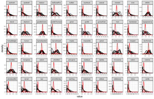
(a) Subposterior estimates of the species pseudoguessing

(b) Species pseudoguessing vs the proportion of correct classification

Figure 9: (a) Comparisons of the posterior distributions of the species pseudoguessing in the subsets and compared to the combined estimate (in red color). (b) Posterior mean and highest density interval of the species pseudoguessing vs the proportion of correct classification. The size of the dots represent the number of times the species appeared in the images for classification.

Site-related difficulties were also produced. Images from some sites were harder to classify; see for instance C05 in Fig.10(a). A comparison between the 225 sites subposterior estimates among the 10 shards is presented in Fig.S.16. These results indicate a high degree of agreement between site difficulties obtained from the different subsets and compared to the consensus values.

In Fig 10(b) we show the posterior estimates of the site difficulties as a function of the proportion of correct classification and the Voronoi diagram of the site difficulties. Sites with a larger difficulty estimate could indicate camera-related problems or installation issues.

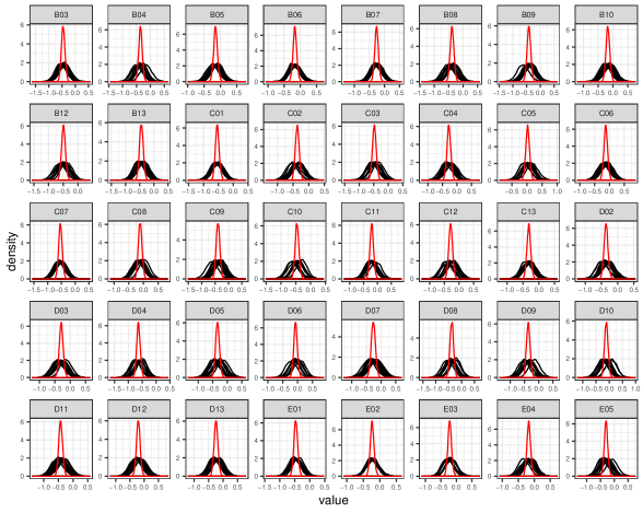
(a) Subposterior estimates of the site difficulties

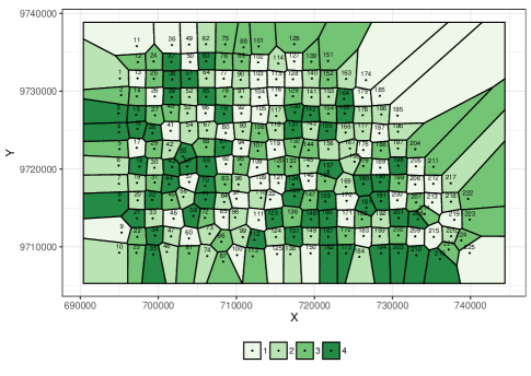
(b) Site difficulties vs the proportion of correct classification

Figure 10: (a) Comparisons of the difficulties posterior estimates in the first 40 sites in the subsets and compared to the consensus estimate. (b) Voronoi diagram of the posterior estimates of the site-related difficulties. Four categories were obtained using the quantiles where dark (light) green represent more difficult (easier) sites. Dots represent the location of the camera.

5 Discussion and conclusion

Networks with millions of contributors worldwide scattered in space and time engage in citizen science activities. This force is helping to reach the United Nations Sustainable Development Goals [42, 32]. In the ecological context, citizens’ contribution is two-fold: providing images, videos and audio files from animals, plants, etc.; but also producing classifications for estimating the distribution of species and for training machine learning algorithms. Yet, the data produced by citizens and hence by these programs are generally inaccurate and/or imprecise, which has received a lot of attention in recent years. Prior research has also noted the importance of measuring the contribution of the subjects to citizen science projects [84]. Although item-response models provide a natural framework in which to investigate and perhaps adjust for these challenges, the literature is limited on their usefulness for crowdsourced programs and particularly in the ecological context.

In this research, we introduced a new methodology and family of IRT models specially tailored for ecological applications. These methods can be used in a wide range of applications involving datasets elicited via crowdsourcing. We focus on ecological spatial data frequently collected in citizen science applications and specifically on citizen-elicited annotations of images. We discuss the application of these models for real-world data, specifically in the presence of inconveniently large datasets. We found that our proposed framework of modeling outperforms the benchmark method in terms of precision and accuracy in a simulation experiment considering factors like the number of geotagged locations, the number of participants, etc. Similarly, our approach performed better for real-life data. The application of the divide-and-recombine approach for massive item response problems is novel and can be translated and extended to other settings.

Our methodology provides a better way of assessing the proficiency of the participants, which is useful for comparing them on equal grounds, for measuring their contribution, for building reputation schemes and for compensation purposes. It also identifies challenging and commonly misclassified classes of responses (e.g. species) in order to produce better guidance, qualifications and users’ training. Obtaining difficulties associated with images gives indications of cameras technical malfunctioning, misplacement, light conditions, etc. We are currently developing the R package staircase (STAtistical Item Response models for Citizen Science applications in Ecology) that will allow practitioners to fit these new family of item response models, producing estimates of the participants’ abilities along with other relevant ecological measures. The package adopts the Bayesian modeling framework and puts particular emphasis on big data.

In our models, participants’ abilities were considered to be constant across the classification period. This is reasonable since the period is generally short for many citizen science projects. However, in some circumstances this condition does not hold, e.g. an increased level of skill is achieved with time as participants learn and train. Consequently, variations like those suggested in Martin and Quinn [58], Dunson [26], Wang et al. [93] and Weng et al. [97] can be adopted. Furthermore, other methods accounting for the participants’ reaction times could also be explored Zhan et al. [e.g. 101], Fox [e.g. 31]. Potential extensions of this particular case study based on the classification of camera traps images include accounting for covariates affecting the species difficulties such as the presence of young specimens or captured while moving. Our case study involves a relatively small geographical scale. Further work should consider items collected over broader scales surveys, at countries and continents levels, or even globally).

Camera-specific parameters and time of the day that also impact the quality of the photograph could be included as a factor in the model. In terms of scalability, variational approximations could be used to speed up the computation on big datasets [66, 43]. We are currently exploring an online updating approach for processing data as it becomes available [82, 81, 14].

Author Contributions

ESF and KM conceptualized, designed the study and drafted the manuscript. ESF wrote the R codes. Both authors made a substantial contribution and approved the final submission.

SUPPLEMENTARY MATERIAL

The supplementary material includes the following file:

Simulations results and posterior estimates obtained via consensus Monte Carlo.

Data and codes availability

The dataset and the R/Stan codes used in the case study (Section  4.3) can be found in the repository: https://github.com/EdgarSantos-Fernandez/staircase. The following files are included:

serengeti.RDS

: contains the Serengeti data set.

Item_response_modeling_for_big_data.Rmd

: this R markdown file includes the full R/Stan codes for fitting the models, combining the posterior estimates and for visualizing the results.

Item_response_modeling_for_big_data.pdf

: this is the knitted R markdown output file.

S.6 SUPPLEMENTARY MATERIAL: Simulations results and posterior estimates obtained via consensus Monte Carlo

Summary: This is the supplementary material for Bayesian item response models for citizen science ecological data and it is composed of two sections. Section S.6 contains information supporting the simulation study. Some results regarding the Case Study are presented in Section S.6.2.

Fig.11(a) and 11(b) depict the posterior distributions violin and boxplots for the abilities in both models (3PL vs 3PLUS) as a function of the true fixed value given by the red dots.

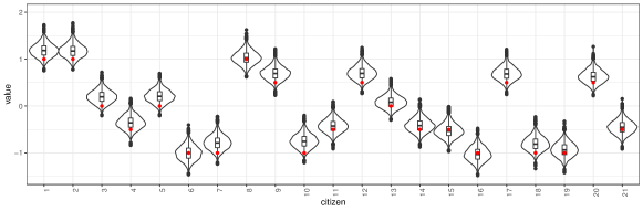
(a) 3PL

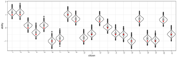
(b) 3PLUS

Figure S.11: Violin/box plot of the posterior distribution of the five groups of users’ abilities $\theta_{j}$ in the 3PL (a) and 3PLUS model (b). The red dots represent the fixed true abilities.

Table S.2: Posterior summary statistics of the regression model for the $\log(\textrm{RMSE}_{\textrm{diff}})$.

Parameter	Rhat	n_eff	mean	sd	se_mean	2.5%	50%	97.5%
$b_{\textrm{Intercept}}$	1.0012	3614	-0.2905	0.0786	0.0013	-0.4452	-0.2912	-0.1376
$b_{\textrm{model3PLUS}}$	1.0006	3035	-0.4437	0.0429	0.0008	-0.5275	-0.4439	-0.3602
$b_{\textrm{neli}}$	1.0003	5022	-0.0088	0.0027	0.0000	-0.0141	-0.0088	-0.0035
$b_{min_{clas}}$	0.9999	3226	-0.0021	0.0077	0.0001	-0.0170	-0.0022	0.0128
$b_{n_{cit}}$	0.9994	5967	-0.0086	0.0010	0.0000	-0.0106	-0.0086	-0.0066
$b_{n}$	1.0015	4111	0.0003	0.0001	0.0000	0.0001	0.0003	0.0005
$\sigma$	1.0010	2558	0.2774	0.0156	0.0003	0.2487	0.2766	0.3099
log-posterior	1.0016	1590	-28.1311	1.8649	0.0468	-32.6632	-27.8176	-25.5008

S.6.1 Simulations results.

In section 3.2 we performed a simulation study to compare both models.

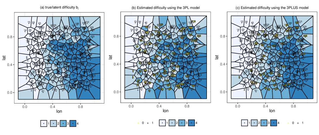
Figure S.12: (a) Voronoi diagram of the latent spatially correlated item difficulties $b_{j}$. The color represents the difficulty category given by the quantiles {[-2.178, -0.514], (-0.514, 0.232], (0.232, 0.814], (0.814, 1.982]} so that each category is composed of approximately 56 locations. The easiest and hardest groups are 1 and 4 respectively. (b) and (c) are the estimated item difficulties in the traditional 3PL and in the 3PLUS model. The yellow labels represent incorrect category estimation.

S.6.2 Posterior estimates obtained from the subposteriors via consensus Monte Carlo.

In the case study (section 4.3), we split the big dataset and fit the Bayesian item response model to each of the individual shards. Fig S.13 shows a comparison of the ability estimates in the 10 shards and those obtained from the consensus Monte Carlo approach.

Similar comparisons are shown in Fig S.14, S.15 and S.16 for the difficulties associated to the species, the pseudoguessing and the site difficulties respectively.

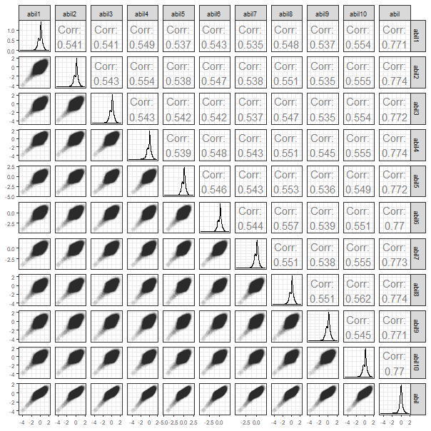
Figure S.13: Comparison of the posterior estimates in the 21,347 users abilities in the shards and from the consensus approach.

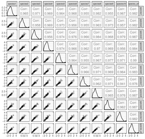
Figure S.14: Comparisons of the posterior estimates of the species difficulties in the shards and from the consensus approach (species_all).

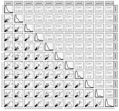
Figure S.15: Comparisons of the posterior means estimates of the species pseudoguessing in the subsets and compared to the combined estimate (guess_all).

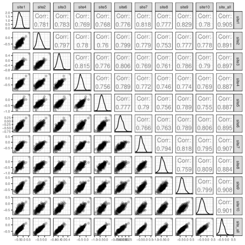
Figure S.16: Comparisons of the difficulties posterior estimates in the 10 subsets (site1, site2, etc) and compared to the consensus estimate (site_all).

Table S.3 shows the consensus posterior estimates for some of the parameters of interest.

Table S.3: Posterior estimates of some of the parameters via consensus Monte Carlo.

	param	id	mean	sd	med	$q_{2.5}$	$q_{97.5}$
1	diff_species_3	baboon	-0.802	0.229	-0.807	-1.251	-0.331
2	diff_species_24	hyenaStriped	2.007	0.734	1.902	0.842	3.697
3	diff_species_26	impossible	4.535	0.614	4.495	3.433	5.898
4	diff_species_30	lionFemale	-0.046	0.267	-0.046	-0.585	0.482
5	diff_species_49	zebra	-2.020	0.180	-2.019	-2.390	-1.671
6	diff_site_1	B03	-0.456	0.214	-0.456	-0.882	-0.023
7	diff_site_2	B04	-0.359	0.216	-0.360	-0.788	0.085
8	diff_site_3	B05	-0.151	0.190	-0.150	-0.527	0.237
9	diff_site_4	B06	-0.167	0.183	-0.169	-0.526	0.208
10	pseudoguessing_3	baboon	0.137	0.083	0.127	0.009	0.322
11	pseudoguessing_24	hyenaStriped	0.230	0.100	0.241	0.019	0.397
12	pseudoguessing_26	impossible	0.010	0.009	0.007	0.000	0.034
13	pseudoguessing_30	lionFemale	0.366	0.074	0.373	0.203	0.497
14	pseudoguessing_49	zebra	0.009	0.009	0.007	0.000	0.032
15	abil_1	1ee963bb67658ec7fb7ff5568f2e5c52	1.016	0.587	0.981	-0.052	2.288
16	abil_2	43047c40867c00a83d0a3982f12f515b	-0.446	0.822	-0.443	-2.128	1.191
17	abil_3	52a791d0b1715d3a64e3304853d78c7c	1.019	0.386	0.978	0.353	1.893
18	abil_4	6ed2e808d62f729c45912856bffb1ae7	0.000	0.592	-0.040	-1.067	1.315
19	abil_5	80c3e443a01284ce8be767b3b68b921d	1.176	0.354	1.143	0.555	1.958
20	abil_6	b1132cb9f684ac9bf8b08522c7537ea6	-0.041	0.528	-0.069	-1.020	1.122
21	abil_7	cb7671ced14ad6f669a2601b249e0e93	-1.407	0.580	-1.402	-2.594	-0.252
22	abil_8	cb93d3701ea002dd736828eb1a87cb88	-0.880	0.616	-0.884	-2.107	0.363
23	abil_9	e6b9208fb9d03ce1c3885fbb866a39f8	0.226	0.458	0.200	-0.620	1.200

References

- Albert [2015] Albert, J. (2015) Introduction to Bayesian item response modelling. International Journal of Quantitative Research in Education, 2, 178–193.
- Albert [1992] Albert, J. H. (1992) Bayesian estimation of normal ogive item response curves using Gibbs sampling. Journal of Educational Statistics, 17, 251–269.
- Altwegg and Nichols [2019] Altwegg, R. and Nichols, J. D. (2019) Occupancy models for citizen-science data. Methods in Ecology and Evolution, 10, 8–21.
- Arab and Courter [2015] Arab, A. and Courter, J. R. (2015) Spatio-temporal trend analysis of spring arrival data for migratory birds. Communications in Statistics-Simulation and Computation, 44, 2535–2547.
- Arab et al. [2016] Arab, A., Courter, J. R. and Zelt, J. (2016) A spatio-temporal comparison of avian migration phenology using citizen science data. Spatial Statistics, 18, 234–245.
- Baker and Kim [2004] Baker, F. B. and Kim, S.-H. (2004) Item response theory: Parameter estimation techniques. CRC Press.
- Besag et al. [1991] Besag, J., York, J. and Mollié, A. (1991) Bayesian image restoration, with two applications in spatial statistics. Annals of the Institute of Statistical Mathematics, 43, 1–20.
- Bird et al. [2014] Bird, T. J., Bates, A. E., Lefcheck, J. S., Hill, N. A., Thomson, R. J., Edgar, G. J., Stuart-Smith, R. D., Wotherspoon, S., Krkosek, M., Stuart-Smith, J. F., Pecl, G. T., Barrett, N. and Frusher, S. (2014) Statistical solutions for error and bias in global citizen science datasets. Biological Conservation, 173, 144 – 154. URL: http://www.sciencedirect.com/science/article/pii/S0006320713002693.
- Birnbaum [1968] Birnbaum, A. L. (1968) Some latent trait models and their use in inferring an examinee’s ability. In Statistical theories of mental test scores. Addison-Wesley.
- Bonney et al. [2009] Bonney, R., Cooper, C. B., Dickinson, J., Kelling, S., Phillips, T., Rosenberg, K. V. and Shirk, J. (2009) Citizen science: a developing tool for expanding science knowledge and scientific literacy. BioScience, 59, 977–984.
- Bonney et al. [2014] Bonney, R., Shirk, J. L., Phillips, T. B., Wiggins, A., Ballard, H. L., Miller-Rushing, A. J. and Parrish, J. K. (2014) Next steps for citizen science. Science, 343, 1436–1437.
- Bürkner [2019] Bürkner, P.-C. (2019) Bayesian Item Response Modelling in R with brms and Stan. arXiv preprint arXiv:1905.09501.
- Cai et al. [2016] Cai, L., Choi, K., Hansen, M. and Harrell, L. (2016) Item response theory. Annual Review of Statistics and Its Application, 3, 297–321. URL: https://doi.org/10.1146/annurev-statistics-041715-033702.
- Callaghan et al. [2019a] Callaghan, C. T., Poore, A. G., Major, R. E., Rowley, J. J. and Cornwell, W. K. (2019a) Optimizing future biodiversity sampling by citizen scientists. Proceedings of the Royal Society B, 286, 20191487.
- Callaghan et al. [2019b] Callaghan, C. T., Rowley, J. J., Cornwell, W. K., Poore, A. G. and Major, R. E. (2019b) Improving big citizen science data: Moving beyond haphazard sampling. PLOS Biology, 17, e3000357.
- Cançado et al. [2016] Cançado, A. L., Gomes, A. E., da Silva, C. Q., Oliveira, F. L. and Duczmal, L. H. (2016) An item response theory approach to spatial cluster estimation and visualization. Environmental and Ecological Statistics, 23, 435–451.
- Carpenter et al. [2017] Carpenter, B., Gelman, A., Hoffman, M. D., Lee, D., Goodrich, B., Betancourt, M., Brubaker, M., Guo, J., Li, P. and Riddell, A. (2017) Stan: A probabilistic programming language. Journal of Statistical Software, 76.
- Chalmers [2012] Chalmers, R. P. (2012) mirt: A multidimensional item response theory package for the R environment. Journal of Statistical Software, 48, 1–29.
- Chambert et al. [2018] Chambert, T., Grant, E. H. C., Miller, D. A., Nichols, J. D., Mulder, K. P. and Brand, A. B. (2018) Two-species occupancy modelling accounting for species misidentification and non-detection. Methods in Ecology and Evolution, 9, 1468–1477.
- Choy et al. [2009] Choy, S. L., O’Leary, R. and Mengersen, K. (2009) Elicitation by design in ecology: using expert opinion to inform priors for bayesian statistical models. Ecology, 90, 265–277.
- Curtis et al. [2010] Curtis, S. M. et al. (2010) BUGS code for item response theory. Journal of Statistical Software, 36, 1–34.
- Datta et al. [2016] Datta, A., Banerjee, S., Finley, A. O. and Gelfand, A. E. (2016) Hierarchical nearest-neighbor Gaussian process models for large geostatistical datasets. Journal of the American Statistical Association, 111, 800–812.
- De Ayala [2013] De Ayala, R. J. (2013) The theory and practice of item response theory. Guilford Publications.
- De Jong et al. [2010] De Jong, M. G., Pieters, R. and Fox, J.-P. (2010) Reducing social desirability bias through item randomized response: An application to measure underreported desires. Journal of Marketing Research, 47, 14–27.
- Dennis et al. [2017] Dennis, E. B., Morgan, B. J., Freeman, S. N., Ridout, M. S., Brereton, T. M., Fox, R., Powney, G. D. and Roy, D. B. (2017) Efficient occupancy model-fitting for extensive citizen-science data. PloS one, 12, e0174433.
- Dunson [2003] Dunson, D. B. (2003) Dynamic latent trait models for multidimensional longitudinal data. Journal of the American Statistical Association, 98, 555–563.
- Embretson and Reise [2013] Embretson, S. E. and Reise, S. P. (2013) Item response theory. Psychology Press.
- Falk et al. [2019] Falk, S., Foster, G., Comont, R., Conroy, J., Bostock, H., Salisbury, A., Kilbey, D., Bennett, J. and Smith, B. (2019) Evaluating the ability of citizen scientists to identify Bumblebee (Bombus) species. PloS one, 14, e0218614.
- Finley et al. [2017] Finley, A. O., Datta, A., Cook, B. C., Morton, D. C., Andersen, H. E. and Banerjee, S. (2017) Applying nearest neighbor Gaussian processes to massive spatial data sets forest canopy height prediction across Tanana Valley Alaska. arXiv preprint arXiv:1702.00434.
- Fischer [1973] Fischer, G. H. (1973) The linear logistic test model as an instrument in educational research. Acta Psychologica, 37, 359–374.
- Fox [2010] Fox, J.-P. (2010) Bayesian item response modeling: Theory and applications. Springer Science & Business Media.
- Fritz et al. [2019] Fritz, S., See, L., Carlson, T., Haklay, M. M., Oliver, J. L., Fraisl, D., Mondardini, R., Brocklehurst, M., Shanley, L. A., Schade, S. et al. (2019) Citizen science and the United Nations Sustainable Development Goals. Nature Sustainability, 2, 922–930.
- Gabry and Mahr [2018] Gabry, J. and Mahr, T. (2018) bayesplot: Plotting for Bayesian Models. URL: https://CRAN.R-project.org/package=bayesplot. R package version 1.6.0.
- Gadermann et al. [2012] Gadermann, A. M., Guhn, M. and Zumbo, B. D. (2012) Estimating ordinal reliability for likert-type and ordinal item response data: a conceptual, empirical, and practical guide. Practical Assessment, Research & Evaluation, 17.
- Garrett et al. [2018] Garrett, R. C., Nar, A. and Fisher, T. J. (2018) ggvoronoi: Voronoi Diagrams and Heatmaps with ’ggplot2’. URL: https://CRAN.R-project.org/package=ggvoronoi. R package version 0.8.2.
- Gold [2016] Gold, C. (2016) Spatial modeling: V oronoi diagrams. International Encyclopedia of Geography: People, the Earth, Environment and Technology: People, the Earth, Environment and Technology, 1–24.
- Grant et al. [2016] Grant, R. L., Furr, D. C., Carpenter, B. and Gelman, A. (2016) Fitting Bayesian item response models in Stata and Stan. arXiv preprint arXiv:1601.03443.
- Gura [2013] Gura, T. (2013) Citizen science: amateur experts. Nature, 496, 259–261.
- Hoffman and Gelman [2014] Hoffman, M. D. and Gelman, A. (2014) The No-U-turn sampler: adaptively setting path lengths in Hamiltonian Monte Carlo. Journal of Machine Learning Research, 15, 1593–1623.
- Howe [2008] Howe, J. (2008) Crowdsourcing: How the power of the crowd is driving the future of business. Random House.
- Hsing et al. [2018] Hsing, P.-Y., Bradley, S., Kent, V. T., Hill, R. A., Smith, G. C., Whittingham, M. J., Cokill, J., Crawley, D., volunteers, M. and Stephens, P. A. (2018) Economical crowdsourcing for camera trap image classification. Remote Sensing in Ecology and Conservation, 4, 361–374.
- Hsu et al. [2014] Hsu, A., Malik, O., Johnson, L. and Esty, D. C. (2014) Development: Mobilize citizens to track sustainability. Nature News, 508, 33.
- Hui et al. [2017] Hui, F. K., Warton, D. I., Ormerod, J. T., Haapaniemi, V. and Taskinen, S. (2017) Variational approximations for generalized linear latent variable models. Journal of Computational and Graphical Statistics, 26, 35–43.
- Humphreys et al. [2019] Humphreys, J. M., Murrow, J. L., Sullivan, J. D. and Prosser, D. J. (2019) Seasonal occurrence and abundance of dabbling ducks across the continental united states: Joint spatio-temporal modelling for the genus anas. Diversity and Distributions, 25, 1497–1508.
- Johnston et al. [2018] Johnston, A., Fink, D., Hochachka, W. M. and Kelling, S. (2018) Estimates of observer expertise improve species distributions from citizen science data. Methods in Ecology and Evolution, 9, 88–97.
- Juhl [2019] Juhl, S. (2019) Measurement uncertainty in spatial models: A Bayesian dynamic measurement model. Political Analysis, 27, 302–319.
- Katzfuss and Cressie [2012] Katzfuss, M. and Cressie, N. (2012) Bayesian hierarchical spatio-temporal smoothing for very large datasets. Environmetrics, 23, 94–107.
- Kelling et al. [2015] Kelling, S., Johnston, A., Hochachka, W. M., Iliff, M., Fink, D., Gerbracht, J., Lagoze, C., La Sorte, F. A., Moore, T., Wiggins, A. et al. (2015) Can observation skills of citizen scientists be estimated using species accumulation curves? PLoS One, 10, e0139600.
- Kohler and Gill [2006] Kohler, K. E. and Gill, S. M. (2006) Coral point count with excel extensions (cpce): A visual basic program for the determination of coral and substrate coverage using random point count methodology. Computers & Geosciences, 32, 1259–1269.
- Kosmala et al. [2018] Kosmala, M., Hufkens, K. and Richardson, A. D. (2018) Integrating camera imagery, crowdsourcing, and deep learning to improve high-frequency automated monitoring of snow at continental-to-global scales. PloS one, 13, e0209649.
- Kosmala et al. [2016] Kosmala, M., Wiggins, A., Swanson, A. and Simmons, B. (2016) Assessing data quality in citizen science. Frontiers in Ecology and the Environment, 14, 551–560.
- Laurens et al. [2012] Laurens, K. R., Hobbs, M., Sunderland, M., Green, M. J. and Mould, G. (2012) Psychotic-like experiences in a community sample of 8000 children aged 9 to 11 years: an item response theory analysis. Psychological Medicine, 42, 1495–1506.
- Lichstein et al. [2002] Lichstein, J. W., Simons, T. R., Shriner, S. A. and Franzreb, K. E. (2002) Spatial autocorrelation and autoregressive models in ecology. Ecological Monographs, 72, 445–463.
- van der Linden and Hambleton [2013] van der Linden, W. J. and Hambleton, R. K. (2013) Handbook of modern item response theory. Springer Science & Business Media.
- van der Linden et al. [2010] van der Linden, W. J., Klein Entink, R. H. and Fox, J.-P. (2010) IRT parameter estimation with response times as collateral information. Applied Psychological Measurement, 34, 327–347.
- Lord [1980] Lord, F. M. (1980) Applications of item response theory to practical testing problems. Hillsdale, NJ:Erlbaum.
- Luo and Jiao [2018] Luo, Y. and Jiao, H. (2018) Using the Stan program for Bayesian item response theory. Educational and Psychological Measurement, 78, 384–408.
- Martin and Quinn [2002] Martin, A. D. and Quinn, K. M. (2002) Dynamic ideal point estimation via Markov chain Monte Carlo for the US Supreme Court, 1953–1999. Political Analysis, 10, 134–153.
- McGann [2014] McGann, A. J. (2014) Estimating the political center from aggregate data: an item response theory alternative to the stimson dyad ratios algorithm. Political Analysis, 22, 115–129.
- McKinley et al. [2017] McKinley, D. C., Miller-Rushing, A. J., Ballard, H. L., Bonney, R., Brown, H., Cook-Patton, S. C., Evans, D. M., French, R. A., Parrish, J. K., Phillips, T. B. et al. (2017) Citizen science can improve conservation science, natural resource management, and environmental protection. Biological Conservation, 208, 15–28.
- Mengersen et al. [2017] Mengersen, K., Peterson, E. E., Clifford, S., Ye, N., Kim, J., Bednarz, T., Brown, R., James, A., Vercelloni, J., Pearse, A. R. et al. (2017) Modelling imperfect presence data obtained by citizen science. Environmetrics, 28, e2446.
- Meyer and Zhu [2013] Meyer, J. P. and Zhu, S. (2013) Fair and equitable measurement of student learning in MOOCs: An introduction to item response theory, scale linking, and score equating. Research & Practice in Assessment, 8, 26–39.
- Miroshnikov and Conlon [2014] Miroshnikov, A. and Conlon, E. (2014) parallelMCMCcombine: Methods for combining independent subset Markov chain Monte Carlo (MCMC) posterior samples to estimate a posterior density given the full data set. URL: https://CRAN.R-project.org/package=parallelMCMCcombine. R package version 1.0.
- Mislevy [1986] Mislevy, R. J. (1986) Bayes modal estimation in item response models. Psychometrika, 51, 177–195.
- Morris et al. [2019] Morris, M., Wheeler-Martin, K., Simpson, D., Mooney, S. J., Gelman, A. and DiMaggio, C. (2019) Bayesian hierarchical spatial models: Implementing the besag york mollié model in stan. Spatial and Spatio-temporal Epidemiology, 31, 100301.
- Natesan et al. [2016] Natesan, P., Nandakumar, R., Minka, T. and Rubright, J. D. (2016) Bayesian prior choice in IRT estimation using MCMC and variational Bayes. Frontiers in Psychology, 7, 1422.
- Neiswanger et al. [2013] Neiswanger, W., Wang, C. and Xing, E. (2013) Asymptotically exact, embarrassingly parallel MCMC. arXiv preprint arXiv:1311.4780.
- Okabe et al. [2009] Okabe, A., Boots, B., Sugihara, K. and Chiu, S. N. (2009) Spatial tessellations: concepts and applications of Voronoi diagrams, vol. 501. John Wiley & Sons.
- Pagel et al. [2014] Pagel, J., Anderson, B. J., O’Hara, R. B., Cramer, W., Fox, R., Jeltsch, F., Roy, D. B., Thomas, C. D. and Schurr, F. M. (2014) Quantifying range-wide variation in population trends from local abundance surveys and widespread opportunistic occurrence records. Methods in Ecology and Evolution, 5, 751–760.
- Patz and Junker [1999] Patz, R. J. and Junker, B. W. (1999) Applications and extensions of mcmc in irt: Multiple item types, missing data, and rated responses. Journal of educational and behavioral statistics, 24, 342–366.
- Pedersen [2019] Pedersen, T. L. (2019) ggforce: Accelerating “ggplot2”. URL: https://CRAN.R-project.org/package=ggforce. R package version 0.2.2.
- Peterson et al. [2020] Peterson, E. E., Santos-Fernández, E., Chen, C., Clifford, S., Vercelloni, J., Pearse, A., Brown, R., Christensen, B., James, A., Anthony, K. et al. (2020) Monitoring through many eyes: Integrating disparate datasets to improve monitoring of the great barrier reef. Environmental Modelling & Software, 124, 104557.
- Peterson et al. [2019] Peterson, E. E., Santos-Fernández, E., Chen, C., Clifford, S., Vercelloni, J., Pearse, A., Brown, R., Christensen, B., James, A., Anthony, K., Loder, J., González-Rivero, M., Roelfsema, C., Caley, M. J., Mellin, C., Bednarz, T. and Mengersen, K. (2019) Monitoring through many eyes: Integrating disparate datasets to improve monitoring of the Great Barrier Reef. Environmental Modelling & Software, 104557.
- Pollock et al. [2014] Pollock, L. J., Tingley, R., Morris, W. K., Golding, N., O’Hara, R. B., Parris, K. M., Vesk, P. A. and McCarthy, M. A. (2014) Understanding co-occurrence by modelling species simultaneously with a Joint Species Distribution Model (JSDM). Methods in Ecology and Evolution, 5, 397–406.
- Purse et al. [2015] Purse, B. V., Comont, R., Butler, A., Brown, P. M., Kessel, C. and Roy, H. E. (2015) Landscape and climate determine patterns of spread for all colour morphs of the alien ladybird harmonia axyridis. Journal of Biogeography, 42, 575–588.
- R Core Team [2018] R Core Team (2018) R: A Language and Environment for Statistical Computing. R Foundation for Statistical Computing, Vienna, Austria. URL: https://www.R-project.org/.
- Rasch [1960] Rasch, G. (1960) Studies in mathematical psychology: I. Probabilistic models for some intelligence and attainment tests. Nielsen & Lydiche. Oxford, England.
- Ratnieks et al. [2016] Ratnieks, F. L., Schrell, F., Sheppard, R. C., Brown, E., Bristow, O. E. and Garbuzov, M. (2016) Data reliability in citizen science: learning curve and the effects of training method, volunteer background and experience on identification accuracy of insects visiting ivy flowers. Methods in Ecology and Evolution, 7, 1226–1235.
- Raykar et al. [2010] Raykar, V. C., Yu, S., Zhao, L. H., Valadez, G. H., Florin, C., Bogoni, L. and Moy, L. (2010) Learning from crowds. Journal of Machine Learning Research, 11, 1297–1322.
- Samejima [1969] Samejima, F. (1969) Estimation of latent ability using a response pattern of graded scores. Psychometrika Monograph Supplement.
- Särkkä [2013] Särkkä, S. (2013) Bayesian filtering and smoothing, vol. 3. Cambridge University Press.
- Schifano et al. [2016] Schifano, E. D., Wu, J., Wang, C., Yan, J. and Chen, M.-H. (2016) Online updating of statistical inference in the big data setting. Technometrics, 58, 393–403.
- Scott et al. [2016] Scott, S. L., Blocker, A. W., Bonassi, F. V., Chipman, H. A., George, E. I. and McCulloch, R. E. (2016) Bayes and big data: The consensus Monte Carlo algorithm. International Journal of Management Science and Engineering Management, 11, 78–88.
- Silvertown et al. [2015] Silvertown, J., Harvey, M., Greenwood, R., Dodd, M., Rosewell, J., Rebelo, T., Ansine, J. and McConway, K. (2015) Crowdsourcing the identification of organisms: A case-study of iSpot. ZooKeys, 125.
- Slowikowski [2019] Slowikowski, K. (2019) ggrepel: Automatically Position Non-Overlapping Text Labels with ’ggplot2’. URL: https://CRAN.R-project.org/package=ggrepel. R package version 0.8.1.
- Stan Development Team [2018] Stan Development Team (2018) RStan: the R interface to Stan. URL: http://mc-stan.org/. R package version 2.18.2.
- Stone and Zhu [2015] Stone, C. A. and Zhu, X. (2015) Bayesian analysis of item response theory models using SAS. Sas Institute.
- Sullivan et al. [2009] Sullivan, B. L., Wood, C. L., Iliff, M. J., Bonney, R. E., Fink, D. and Kelling, S. (2009) ebird: A citizen-based bird observation network in the biological sciences. Biological Conservation, 142, 2282–2292.
- Swanson et al. [2015] Swanson, A., Kosmala, M., Lintott, C., Simpson, R., Smith, A. and Packer, C. (2015) Snapshot Serengeti, high-frequency annotated camera trap images of 40 mammalian species in an African savanna. Scientific Data, 2, 150026.
- Vehtari et al. [2017] Vehtari, A., Gelman, A. and Gabry, J. (2017) Practical Bayesian model evaluation using leave-one-out cross-validation and WAIC. Statistics and Computing, 27, 1413–1432.
- Ver Hoef et al. [2018] Ver Hoef, J. M., Peterson, E. E., Hooten, M. B., Hanks, E. M. and Fortin, M.-J. (2018) Spatial autoregressive models for statistical inference from ecological data. Ecological Monographs, 88, 36–59.
- Wang et al. [2016] Wang, C., Chen, M.-H., Schifano, E., Wu, J. and Yan, J. (2016) Statistical methods and computing for big data. Statistics and its Interface, 9, 399.
- Wang et al. [2013] Wang, X., Berger, J. O., Burdick, D. S. et al. (2013) Bayesian analysis of dynamic item response models in educational testing. The Annals of Applied Statistics, 7, 126–153.
- Warton et al. [2015] Warton, D. I., Blanchet, F. G., O’Hara, R. B., Ovaskainen, O., Taskinen, S., Walker, S. C. and Hui, F. K. (2015) So many variables: joint modeling in community ecology. Trends in Ecology & Evolution, 30, 766–779.
- Watanabe [2010] Watanabe, S. (2010) Asymptotic equivalence of bayes cross validation and widely applicable information criterion in singular learning theory. Journal of Machine Learning Research, 11, 3571–3594.
- Wauters et al. [2010] Wauters, K., Desmet, P. and Van Den Noortgate, W. (2010) Adaptive item-based learning environments based on the item response theory: possibilities and challenges. Journal of Computer Assisted Learning, 26, 549–562.
- Weng et al. [2018] Weng, R. C.-H., Coad, D. S. et al. (2018) Real-time Bayesian parameter estimation for item response models. Bayesian Analysis, 13, 115–137.
- Wickham [2017] Wickham, H. (2017) tidyverse: Easily Install and Load the ’Tidyverse’. URL: https://CRAN.R-project.org/package=tidyverse. R package version 1.2.1.
- Willi et al. [2019] Willi, M., Pitman, R. T., Cardoso, A. W., Locke, C., Swanson, A., Boyer, A., Veldthuis, M. and Fortson, L. (2019) Identifying animal species in camera trap images using deep learning and citizen science. Methods in Ecology and Evolution, 10, 80–91.
- Wilson et al. [2008] Wilson, M., De Boeck, P. and Carstensen, C. H. (2008) Explanatory item response models: A brief introduction. Assessment of Competencies in Educational Contexts, 91–120.
- Zhan et al. [2018] Zhan, P., Jiao, H. and Liao, D. (2018) Cognitive diagnosis modelling incorporating item response times. British Journal of Mathematical and Statistical Psychology, 71, 262–286.
- Zhang et al. [2013] Zhang, J., Huang, K., Cottman-Fields, M., Truskinger, A., Roe, P., Duan, S., Dong, X., Towsey, M. and Wimmer, J. (2013) Managing and analysing big audio data for environmental monitoring. In 2013 IEEE 16th International Conference on Computational Science and Engineering, 997–1004. IEEE.