RC Circuits based Distributed Conditional Gradient Method

Abstract

We consider distributed optimization on undirected connected graphs. We propose a novel distributed conditional gradient method with $O(1/\sqrt{k})$ convergence. Compared with existing methods, each iteration of our method uses both communication and linear minimization step only once rather than multiple times. We further extend our results to cases with composite local constraints. We demonstrate our results via examples on distributed matrix completion problem.

I Introduction

Distributed optimization aims to optimize sum of convex functions via only local computation and communication on a connected graph $\mathcal{G}$ with node set $\mathcal{V}$ and edge set $\mathcal{E}$ [1, 2], which takes the following form,

$$\begin{array}[]{ll}\underset{x_{1},\ldots,x_{|\mathcal{V}|}}{\mbox{minimize}}&\sum_{i\in\mathcal{V}}f_{i}(x_{i})\\ \mbox{subject to}&x_{i}=x_{j},\enskip\forall\{ij\}\in\mathcal{E},\\ &x_{i}\in X_{i},\enskip\forall i\in\mathcal{V}.\end{array}$$ (1)

where $f_{i}$ and $X_{i}$ are respectively the convex objective function and convex feasible set available to node $i$ only. Problem (1) arises frequently from multi-agent applications such as distributed tracking and estimation [3, 4, 5].

Many distributed optimization algorithms have been developed to solve (1). To ensure each local variable $x_{i}$ remains in constraint set $X_{i}$, different algorithms use different oracles–computation subroutines called at each iteration–on each node $i\in\mathcal{V}$. We list three of the most popular ones, where $c_{i}$ denotes certain constants:

$$\mathbf{prox}(c_{i})= \mathop{\rm argmin}_{x_{i}\in X_{i}}\,\,f_{i}(x_{i})+\textstyle\frac{\rho}{2}\left\lVert x_{i}-c_{i}\right\rVert_{2}^{2},$$ (2a)

$$\mathbf{proj}(c_{i})= \mathop{\rm argmin}_{x_{i}\in X_{i}}\,\,\textstyle\frac{1}{2}\left\lVert x_{i}-c_{i}\right\rVert_{2}^{2},$$ (2b)

$$\mathbf{lm}(c_{i})= \mathop{\rm argmin}_{x_{i}\in X_{i}}\,\,\langle c_{i},x_{i}\rangle.$$ (2c)

The first one is the proximal oracle given by (2a) with $\rho>0$, which is widely used by distributed Alternating Direction Method of Multipliers (ADMM) [6, 7, 8]. Since exact evaluation of a proximal oracle may require an iterative algorithm itself, distributed ADMM is usually difficult to implement. A more efficient alternative is the projection oracle given by (2b). Such an oracle minimizes the quadratic distance to a reference point $c_{i}$. Typical algorithms using projection oracle are distributed projected subgradient methods [9, 10, 11]. We note that the quadratic function in proximal and projection oracles can be further generalized to Bregman divergence of strongly convex function [12, 13, 14, 15, 16, 17].

Another oracle that recently become popular is the linear minimization oracle given by (2c), which, instead of the quadratic function in (2b), optimizes a linear function. First proposed in conditional gradient method (a.k.a Frank–Wolfe method) [18], such oracle lately received renewed interest due to its computation efficiency over the convex hulls of an atomic set [19, 20, 21]. Algorithms that solve problem (1) using oracle (2c) are commonly known as distributed conditional gradient method [22, 23, 24, 25].

However, the existing distributed conditional gradient methods have the following limitations. The algorithm in [24] assumes the underlying graph $\mathcal{G}$ has a master-slave hierarchy, which is sensitive to node failure. The algorithms proposed in [22, 23, 25] relaxed this assumption, but each iteration of the resulting algorithm either uses multiple (at least two) communication steps until a consensus condition is reached [22, 23], or multiple linear minimization steps until an optimality condition is reached [25]. These observations motivate the following question:

Is it possible to design a distributed conditional gradient method that uses both communication and linear minimization step only once per iteration?

In this work, we answer this question affirmatively and make the following contributions.

1. We propose a novel distributed conditional gradient method with $O(1/\sqrt{k})$ convergence. Compared with existing methods [23, 25], our method uses both communication and linear minimization step once per iteration rather than multiple times, and allows approximate linear minimization oracles.

2. We further extend our results to problems with composite local constraints by combining linear minimization oracle and projection oracle together, which allows more efficient computation than either oracle alone.

Our work combines ideas from conditional-gradient based augmented Lagrangian methods [26, 27] and physics inspired distributed algorithms [28, 29]. The rest of the paper is organized as follows. After the preliminaries in Section II, we present our algorithm and its convergence proof in Section III and Section IV, then further extend them to composite constraint case in Section V. We then demonstrate our results via numerical examples in Section VI before conclude in Section VII.

II Preliminaries

Let $\mathbb{R}$ denote the real numbers, $\mathbb{R}^{n}$ the $n$-dimensional real numbers. We use $\cdot^{\top}$ to denote matrix (and vector) transpose. Let $\langle x,y\rangle=x^{\top}y$ and $\left\lVert x\right\rVert_{2}=\sqrt{\langle x,x\rangle}$ denote the inner product and, respectively, its induced norm. Let $I_{n}$ denotes the $n\times n$ identity matrix and $\otimes$ denote Kronecker product.

II-A Graph theory

An undirected graph $\mathcal{G}=(\mathcal{V},\mathcal{E})$ consists of a node set $\mathcal{V}$ and an edge set $\mathcal{E}$, where an edge is a pair of distinct nodes in $\mathcal{V}$. For an arbitrary orientation on $\mathcal{G}$, i.e., each edge has a head and a tail, the $|\mathcal{V}|\times|\mathcal{E}|$ incidence matrix is denoted by $\overline{E}(\mathcal{G})$. The columns of $\overline{E}(\mathcal{G})$ are indexed by the edges in $\mathcal{E}$, and the entry on their $i$-th row takes the value “$1$” if node $i$ is the head of the edge, “$-1$” if it is its tail, and $0$ otherwise. When graph $\mathcal{G}$ is connected, the nullspace of $\overline{E}(\mathcal{G})^{\top}$ is spanned by vector of all $1$’s.

II-B Convex Analysis

Let $X\subseteq\mathbb{R}^{n}$ denote a closed convex set. A continuously differentiable function $f:\mathbb{R}^{n}\to\mathbb{R}$ is convex if and only if, for all $x,x^{\prime}\in\mathbb{R}^{n},$

$$f(x^{\prime})\geq f(x)+\langle\nabla f(x),x^{\prime}-x\rangle.$$ (3)

We say a convex function $f$ is $\beta$-smooth if $\frac{\beta}{2}\left\lVert\cdot\right\rVert_{2}^{2}-f$ is also convex, which implies the following [30, Thm. 2.1.5]

$$f(x^{\prime})\leq \textstyle f(x)+\langle\nabla f(x),x^{\prime}-x\rangle+\frac{\beta}{2}\left\lVert x^{\prime}-x\right\rVert_{2}^{2},$$ (4a)

$$f(x^{\prime})\geq \textstyle f(x)+\langle\nabla f(x),x^{\prime}-x\rangle+\frac{1}{2\beta}\left\lVert\nabla f(x^{\prime})-\nabla f(x)\right\rVert_{2}^{2}.$$ (4b)

The normal cone $N_{X}(x)$ at $x\in X$ is given by

$$N_{X}(x)=\{u|\,\langle u,x^{\prime}-x\rangle\leq 0,\forall x^{\prime}\in X\}.$$ (5)

The projection map $P_{X}$ onto set $X$ is given by

$$P_{X}(x)=\textstyle\mathop{\rm argmin}_{y\in X}\textstyle\frac{1}{2}\left\lVert x-y\right\rVert^{2}_{2}.$$ (6)

III Algorithm

We present our main algorithm in this section, which is inspired by RC circuits dynamics. Throughout, we assume graph $\mathcal{G}=(\mathcal{V},\mathcal{E})$ is undirected and connected. We also define the following matrices based on graph $\mathcal{G}$

$$E(\mathcal{G})=\overline{E}(\mathcal{G})\otimes I_{n},\enskip L(\mathcal{G})=(\overline{E}(\mathcal{G})\overline{E}(\mathcal{G})^{\top})\otimes I_{n}.$$ (7)

With these definitions, we can rewrite the optimization template (1) in the following form

$$\begin{array}[]{ll}\underset{x}{\mbox{minimize}}&f(x)=\sum_{i\in\mathcal{V}}f_{i}(x_{i})\\ \mbox{s.t.}&E(\mathcal{G})^{\top}x=0,\enskip x\in X=\prod_{i=1}^{|\mathcal{V}|}X_{i}\end{array}$$ (8)

where $x=[x_{1}^{\top},\ldots,x_{|\mathcal{V}|}^{\top}]^{\top}$ and $\prod_{i=1}^{|\mathcal{V}|}X_{i}$ is the Cartesian product of $X_{1},\ldots,X_{|\mathcal{V}|}$. We assume, for all $i\in\mathcal{V}$, that $f_{i}$ is convex and differentiable, $X_{i}\subset\mathbb{R}^{n}$ is convex and compact.

Figure 1: An illustration of RC circuits

Aiming to design a distributed algorithm for problem (8), we consider a conceptual RC circuits model defined on graph $\mathcal{G}=(\mathcal{V},\mathcal{E})$ as follows. Let each node $i\in\mathcal{V}$ denote a pin with electrical potential $x_{i}(t)$ at time $t$. We add a linear capacitor with unit capacitance in parallel with a nonlinear resistor which maps potential $x_{i}$ to $\nabla f_{i}(x_{i})$ between each pin $i$ and ground (zero potential point), then add a linear resistor with time varying resistance $1/r(t)$ on each edge $\{ij\}\in\mathcal{E}$ where $r(t)>0$ and $\lim_{t\to\infty}1/r(t)=0$. See Fig. 1 and Table I for an illustration.

TABLE I: Voltage-current relation of RC units

type	symbol	voltage	current
non-linear resistor		$x_{i}$	$\nabla f_{i}(x_{i})$
linear resistor		$x_{i}-x_{j}$	$r(x_{i}-x_{j})$
capacitor		$x_{i}$	$\frac{d}{dt}x_{i}$

As the resistance on edges decreases to zero, i.e., $1/r(t)\to 0$, the potential value on neighboring nodes necessarily reaches the same, i.e.,

$$x_{i}(t)-x_{j}(t)\to 0,\enskip\forall\{ij\}\in\mathcal{E}.$$ (9)

Further, if the circuits are reaching an equilibrium where $\frac{d}{dt}x_{i}(t)\to 0$ for all $i\in\mathcal{V}$, then applying Kirchoff current law to the collection of all edges gives

$$\textstyle\sum_{i\in\mathcal{V}}\nabla f_{i}(x_{i}(t))\to 0.$$ (10)

Notice that conditions in (9) and (10) are exactly the optimality conditions of (8) when $X=\mathbb{R}^{|\mathcal{V}|n}$, which suggests that the dynamics of the constructed RC circuits may provide a prototype algorithm for problem (8). Following this intuition, we apply Kirchoff current law to pin $i\in\mathcal{V}$ for any $t\geq 0$ (not necessarily at equilibrium) and obtain

$$\textstyle 0=\frac{d}{dt}x_{i}(t)+\nabla f_{i}(x_{i}(t))+r(t)\sum_{j\in\mathcal{N}(i)}(x_{j}(t)-x_{i}(t)),$$ (11)

where $j\in\mathcal{N}(i)$ if and only if $\{ij\}\in\mathcal{E}$. Let $x(t)=[x_{1}(t)^{\top},\ldots,x_{|\mathcal{V}|}(t)^{\top}]^{\top}$ and $f(x)=\sum_{i\in\mathcal{V}}f_{i}(x_{i})$, then we can rewrite (11) for all $i\in\mathcal{V}$ compactly as follows

$$\textstyle\frac{d}{dt}x(t)=-\nabla f(x(t))-r(t)L(\mathcal{G})x(t),$$ (12)

A naive Euler-forward discretization of (12) says that $x^{k+1}$ is obtained by moving $x^{k}$ in the direction of $-\nabla f(x^{k})-r^{k}L(\mathcal{G})x^{k}$. However, it is difficult to choose appropriate step sizes so that $x^{k}\in X$ for all $k$. To remedy this, we propose the following discretization of (12)

$$y^{k}= \mathop{\rm argmin}_{y\in X}\langle\nabla f(x^{k})+r^{k}L(\mathcal{G})x^{k},y\rangle,$$ (RC)

$$x^{k+1}= x^{k}+\alpha^{k}(y^{k}-x^{k}),$$

where $\alpha^{k}\in(0,1]$. Iteration (RC) says that $x^{k+1}$ is obtained by moving $x^{k}$ towards $y^{k}$, which is the extreme point when moving in the direction $-\nabla f(x^{k})-r^{k}L(\mathcal{G})$ without leaving set $X$. Notice that $x^{k+1}$ is a convex combination of $x^{k}$ and $y^{k}$ as $\alpha^{k}\in(0,1]$. Since $X$ is convex, this ensures $x^{k+1}\in X$ whenever $x^{k}\in X$. Hence, algorithm (RC) ensures $x^{k}\in X$ for all $k\geq 1$ as long as $x^{1}\in X$.

Remark 1.

Compared with existing methods, each iteration in algorithm (RC) uses both communication and linear minimization step only once, which is more efficient than the multiple (at least two) communication steps in [23] and multiple linear minimization steps in [25].

In the next section, we will show that algorithm (RC) indeed converges to the optimum of (8). The key challenge is to find an appropriate sequence of step sizes $\{\alpha^{k}\}$ and determine how fast the sequence $\{r^{k}\}$ grows to infinity.

IV Convergence

In this section, we establish the convergence of algorithm (RC) proposed in the previous section, and further extend it to cases with approximate linear minimization. We first group our technical assumptions as follows.

Assumption 1.

1. Graph $\mathcal{G}=(\mathcal{V},\mathcal{E})$ is undirected and connected.

2. For all $i\in\mathcal{V}$, $f_{i}:\mathbb{R}^{n}\to\mathbb{R}$ is continuously differentiable, convex and $\beta$-smooth, i.e., both $f_{i}$ and $\frac{\beta}{2}\left\lVert\cdot\right\rVert_{2}^{2}-f_{i}$ are convex, $X_{i}\subseteq\mathbb{R}^{n}$ is a compact convex set. We assume $\max_{x,x^{\prime}\in X}\left\lVert x-x^{\prime}\right\rVert^{2}_{2}\leq\delta$ for some $\delta>0$ where $X=\prod_{i=1}^{\mathcal{V}}X_{i}$.

Assumption 2.

There exists $x^{\star}\in X$ and $u^{\star}$ such that

$$E(\mathcal{G})^{\top}x^{\star}= 0,$$ (13a)

$$-E(\mathcal{G})u^{\star}-\nabla f(x^{\star})\in N_{X}(x^{\star}).$$ (13b)

Based on these assumptions, the following theorem shows the convergence of (RC) in terms of both the objective function value and consensus error, where we let $\left\lVert L(\mathcal{G})\right\rVert_{2}$ to denote the largest eigenvalue of $L(\mathcal{G})$ (all proofs are delayed to the Appendix).

Theorem 1.

Suppose Assumption 1 and 2 hold. If sequence $\{x^{k}\}$ is generated by (RC) with $\alpha^{k}=\frac{2}{k+1}$, $r^{k}=r^{0}\sqrt{k+1}$ for some $r^{0}>0$, then

$$|f(x^{k})-f(x^{\star})|\leq \textstyle\frac{2\max\{\sigma^{k}\delta^{2},\rho^{2}+\rho\sqrt{\sigma^{k}\delta}\}}{\sqrt{k}},$$

$$\left\lVert E(\mathcal{G})^{\top}x^{k}\right\rVert_{2}\leq \textstyle\frac{2(\rho+\sqrt{\sigma^{k}\delta})}{\sqrt{k}},$$

where $\rho=\left\lVert u^{\star}\right\rVert_{2}$ and $\sigma^{k}=\frac{\beta}{\sqrt{k}}+\left\lVert L(\mathcal{G})\right\rVert_{2}r^{0}$.

Each iteration of (RC) requires an exact linear minimization. However, it is important to note that conditional gradient method itself is known to be robust to approximate linear minimization as well [20]. If we let $y^{\epsilon}$ be an $\epsilon$-optimal solution to $\min_{y\in X}\langle c,y\rangle$ in the following sense

$$\langle c,y^{\epsilon}\rangle-\min_{y\in X}\langle c,y\rangle\leq\epsilon,\enskip y^{\epsilon}\in X.$$ (14)

Then the following corollary shows that if the linear minimization in algorithm (RC) is solved approximatedly in the sense of (14) with increasing accuracy, then convergence results similar to those in Theorem 1 still hold.

Corollary 1.

If the $y^{k}$ used in (RC) is replaced by an $\epsilon^{k}$-optimal solution to the corresponding linear minimization in the sense of (14), then Theorem 1 still holds with $\sigma^{k}=(1+\kappa)(\frac{\beta}{\sqrt{k}}+\left\lVert L(\mathcal{G})\right\rVert_{2}r^{0})$ for some $\kappa>0$ if

$$\textstyle\epsilon^{k}\leq\kappa\big{(}\frac{\beta}{\sqrt{k+1}}+\left\lVert L(\mathcal{G}\right\rVert_{2}r^{0}\big{)}\frac{\delta}{\sqrt{k+1}}.$$

V Distributed Optimization with Composite Local Constraints

One limitation of existing distributed conditional gradient methods [22, 23, 24, 25] is that their iterates require linear minimization over the entire local constraint set, which can be computationally challenging. It also completely discard projection oracles, which may lead to efficient computation in many interesting scenarios [9, 10, 11]. Motivated by these observations, we consider the following extension to problem (8) with composite constraints on each node

$$\begin{array}[]{ll}\underset{x}{\mbox{minimize}}&f(x)=\sum_{i\in\mathcal{V}}f_{i}(x_{i})\\ \mbox{s.t.}&E(\mathcal{G})^{\top}x=0,\\ &x\in X\cap Y=(\prod_{i=1}^{|\mathcal{V}|}X_{i})\cap(\prod_{i=1}^{|\mathcal{V}|}Y_{i})\end{array}$$ (15)

where, in addition to the assumptions we made for (8), we assume $Y_{i}\subseteq\mathbb{R}^{n}$ is a close convex set; we also assume that the projection oracle (2b) is efficient on $Y_{i}$, i.e., $P_{Y_{i}}(x_{i})$ is easy to compute for all $i\in\mathcal{V}$.

To exploit the structure of (15), we propose the following modification to (RC), whose linear minimization contains a penalty term for not only the consensus constraints violation $L(\mathcal{G})x^{k}$ but also the difference between $x^{k}$ and $P_{Y}(x^{k})$.

$$y^{k}= \mathop{\rm argmin}_{y\in X}\langle\nabla f(x^{k})+r^{k}(x^{k}-P_{Y}(x^{k})+L(\mathcal{G})x^{k}),y\rangle,$$ (RC-co)

$$x^{k+1}= x^{k}+\alpha^{k}(y^{k}-x^{k}).$$

Since $Y=\prod_{i=1}^{|\mathcal{V}|}Y_{i}$, it is straightforward to show that

$$P_{Y}(x)=[P_{Y_{1}}(x_{1})^{\top},\ldots,P_{Y_{|\mathcal{V}|}}(x_{|\mathcal{V}|})^{\top}]^{\top},$$ (16)

for any $x=[x_{i}^{\top},\ldots,x_{|\mathcal{V}|}^{\top}]^{\top}$. Hence (RC-co) also allows fully distributed implementation.

We now prove that, with proper modifications to Assumption 2, the results similar to those in Section IV still hold (all proofs are delayed to the Appendix)..

Assumption 3.

For all $i\in\mathcal{V}$, $Y_{i}\subseteq\mathbb{R}^{n}$ is a compact convex set. There exists $x^{\star}\in X$, $u^{\star}$ and $v^{\star}\in N_{Y}(x^{\star})$ such that

$$E(\mathcal{G})^{\top}x^{\star}= 0,$$ (17a)

$$-E(\mathcal{G})u^{\star}-\nabla f(x^{\star})-v^{\star}\in N_{X}(x^{\star}).$$ (17b)

Theorem 2.

Suppose Assumption 1 and 3 hold. If sequence $\{x^{k}\}$ is generated by (RC-co) with $\alpha^{k}=\frac{2}{k+1}$, $r^{k}=r^{0}\sqrt{k+1}$ for some $r^{0}>0$, then

$$|f(x^{k})-f(x^{\star})|\leq \textstyle\frac{2\max\{\sigma^{k}\delta^{2},\rho^{2}+\rho\sqrt{\sigma^{k}\delta}\}}{\sqrt{k}},$$

$$\left\lVert\begin{bmatrix}E(\mathcal{G})^{\top}x^{k}\\ x^{k}-P_{Y}(x^{k})\end{bmatrix}\right\rVert_{2}\leq \textstyle\frac{2(\rho+\sqrt{\sigma^{k}\delta})}{\sqrt{k}},$$

where $\rho=\left\lVert\begin{bmatrix}u^{\star}\\ v^{\star}\end{bmatrix}\right\rVert_{2}$ and $\sigma^{k}=\frac{\beta}{\sqrt{k}}+(\left\lVert L(\mathcal{G})\right\rVert_{2}+1)r^{0}$.

Remark 2.

Algorithm (RC-co) can also be interpreted as a combination of Nestrov smoothing of indicator function and conditional gradient method [26].

Corollary 2.

If the $y^{k}$ used in (RC-co) is replaced by an $\epsilon^{k}$-optimal solution to to the corresponding linear optimization in the sense of (14), then Theorem 2 still holds with $\sigma^{k}=(1+\kappa)(\frac{\beta}{\sqrt{k}}+(\left\lVert L(\mathcal{G})\right\rVert_{2}+1)r^{0})$ for some $\kappa>0$ if

$$\textstyle\epsilon^{k}\leq\kappa\big{(}\frac{\beta}{\sqrt{k+1}}+(\left\lVert L(\mathcal{G}\right\rVert_{2}+1)r^{0}\big{)}\frac{\delta}{\sqrt{k+1}}.$$

VI Numerical Examples

Distributed matrix completion aims to predict missing entries of a low rank target matrix using corrupted partial measurements distributed over a network $\mathcal{G}=(\mathcal{V},\mathcal{E})$ [31, 23]. Here we consider a template of the following form,

$$\begin{array}[]{ll}\underset{x_{1},\ldots,x_{|\mathcal{V}|}\in\mathbb{R}^{n\times n}}{\mbox{minimize}}&\sum_{i\in\mathcal{V}}\left\lVert o_{i}\odot(x_{i}-d)\right\rVert_{F}^{2}\\ \mbox{s.t.}&x_{i}=x_{j},\enskip\forall\{ij\}\in\mathcal{E},\\ &\left\lVert x_{i}\right\rVert_{*}\leq\theta,\enskip x_{i}=x_{i}^{\top},\enskip\forall i\in\mathcal{V},\\ &l_{i}\leq x_{i}\leq u_{i},\enskip\forall i\in\mathcal{V}.\end{array}$$ (18)

where $\odot,\left\lVert\cdot\right\rVert_{F},\left\lVert\cdot\right\rVert_{*}$ denote the Hadamard (entry-wise) product, Frobenius norm and nuclear norm, $d\in\mathbb{R}^{n\times n}$ is a measurement of the target matrix. Further, for all $i\in\mathcal{V}$, $o_{i}\in\mathbb{R}^{n\times n}$ is a (0,1)-matrix whose sparsity pattern shows which measurements are available on node $i$; $l_{i},u_{i}\in\mathbb{R}^{n\times n}$ are entry-wise upper and lower bound matrices. Note that the constraint $\left\lVert x_{i}\right\rVert_{*}\leq\theta$ with $\theta>0$ aims to promote low rank solutions [23]. Let $f_{i}(x_{i})=\left\lVert o_{i}\odot(x_{i}-d)\right\rVert_{F}^{2}$, $X_{i}=\{x_{i}|\left\lVert x_{i}\right\rVert_{*}\leq\theta,x_{i}=x_{i}^{\top}\}$ and $Y_{i}=\{x_{i}|l_{i}\leq x_{i}\leq u_{i}\}$, then problem (18) fits the template (15) in Section V.

We consider an example of (18) that estimates pairwise node distance based on partial noisy measurements on a random geometric graph as follows [32]. We first uniformly sample $|\mathcal{V}|=10$ position vectors $p_{1},\ldots,p_{|\mathcal{V}|}\in[0,1]^{3}$. Then define $\mathcal{G}$ by letting $\{ij\}\in\mathcal{E}$ if $\left\lVert p_{i}-p_{j}\right\rVert_{2}\leq 0.6$. Let the $ij$-th entry of $d$ be $\left\lVert p_{i}-p_{j}\right\rVert_{2}+\xi_{ij}$ where $\xi_{ij}$ is sampled from the normal distribution with zero-mean and variance $0.01$. For all $i\in\mathcal{V}$, let the $ij$-th and $ji$-th entry be $1$ if $\{ij\}\in\mathcal{E}$ and zero elsewhere; let $l_{i}$ to be a zero matrix; let off-diagonal entries in $u_{i}$ be $3$ and diagonal ones be $0$.

We test our algorithm (RC-co) on such example along with two benchmark methods, distributed projected gradient method (dist. Proj.) [9] and distributed conditional gradient method (dist. CG) [23], see Figure 2. The convergence of our method is similar to that of the two benchmark methods [9, 23]. However, the benchmark methods use either linear minimization or projection over set $X\cap Y$–to our best knowledge, neither oracle admits efficient solution in our example. In comparison, each iteration of (RC-co) uses linear minimization over $X$, which can be computed very efficiently using Lanczo’s algorithm (see [20, Sec. 4.3] for a detailed discussion), and projection onto $Y$, which amounts to computing entry-wise max/min. Hence the per-iteration computation of our method is much more efficient compared with methods in [9, 23]. The price for such efficiency is that, rather than ensuring $x^{k}\in Y$, our method only ensures $x^{k}$ converges to $Y$ in the sense of Theorem 2.

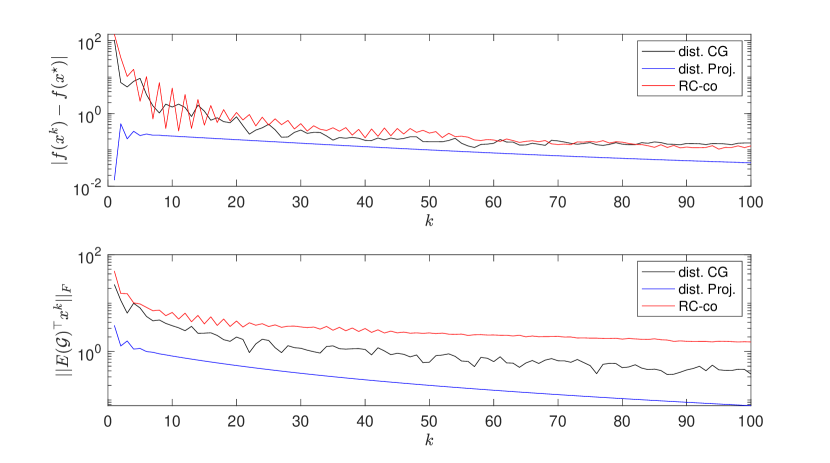
Figure 2: Convergence over iterations.

VII Conclusion

We propose a novel distributed conditional gradient method with $O(1/\sqrt{k})$ convergence rate, and extend our results to composite constraints cases. However, our $O(1/\sqrt{k})$ convergence still mismatches the $O(1/k)$ convergence of the results in [23] and it is still unclear whether alternative circuits model such as RLC circuits [29] can yield better algorithm design. Our future direction will focus on addressing these limitations, and non-convex extensions.

APPENDIX

In this appendix, we first prove Theorem 2 and Corollary 2, then prove Theorem 1 and Corollary 1 by letting $Y=\mathbb{R}^{n|\mathcal{V}|}$. We start with the following lemma.

Lemma 1.

Under the assumptions of Theorem 2, we have

$$f(x^{k})-f(x^{\star})$$

$$\leq \textstyle\frac{2\sigma^{k}\delta}{\sqrt{k}}-\textstyle\frac{\sqrt{k}}{2}(\left\lVert E(\mathcal{G})^{\top}x^{k}\right\rVert_{2}^{2}+\left\lVert x^{k}-P_{Y}(x^{k})\right\rVert_{2}^{2}),$$

where $\sigma^{k}=\frac{\beta}{\sqrt{k}}+(\left\lVert L(\mathcal{G})\right\rVert_{2}+1)r^{0}$.

Proof.

Let

$$d(x)=\textstyle\frac{1}{2}\left\lVert x-P_{Y}(x)\right\rVert_{2}^{2},\enskip g(u)=\textstyle\frac{1}{2}\left\lVert u\right\rVert_{2}^{2}+\max_{y\in Y}\langle u,y\rangle$$ (19)

Since $Y$ is convex and compact, one can show that $d(x)$ is differentiable with $\nabla d(x)=x-P_{Y}(x)$ [33, Ex. 8.53].

In addition, observe that

$$\textstyle\max_{u}\langle u,x\rangle-g(u)= \textstyle\max_{u}-\frac{1}{2}\left\lVert u\right\rVert_{2}^{2}-\max_{y\in Y}\langle u,y-x\rangle$$

$$= \textstyle\max_{u}\min_{y\in Y}-\frac{1}{2}\left\lVert u\right\rVert_{2}^{2}+\langle u,x-y\rangle$$

$$= \textstyle\min_{y\in Y}\max_{u}-\frac{1}{2}\left\lVert u\right\rVert_{2}^{2}+\langle u,x-y\rangle$$

$$= \textstyle\min_{y\in Y}\frac{1}{2}\left\lVert x-y\right\rVert_{2}^{2}=d(x)$$

where we swap the $\max$ and $\min$ since $Y$ is bounded and $-\frac{1}{2}\left\lVert u\right\rVert_{2}^{2}+\langle u,x-y\rangle$ is convex in $y$ and concave in $u$ [34, Cor.37.3.2]. The above equation shows that $d(x)$ is the conjugate of a $1$-strongly convex function $g(u)$ [33, Ex. 12.59 ], hence $d(x)$ is convex and $1$-smooth [33, Prop. 12.60], i.e., $d(x)=\frac{1}{2}\left\lVert x-P_{Y}(x)\right\rVert_{2}^{2}$ satisfies (4) with $\beta=1$.

We define the following quantities.

$$h(x)= \textstyle\frac{1}{2}\left\lVert x-P_{Y}(x)\right\rVert_{2}^{2}+\frac{1}{2}\left\lVert E(\mathcal{G})^{\top}x\right\rVert_{2}^{2},$$ (20a)

$$V^{k}= \textstyle f(x^{k})+r^{k-1}h(x^{k})-f(x^{\star}),$$ (20b)

$$\Delta^{k}= \textstyle\frac{1}{2}(\beta+(\left\lVert L(\mathcal{G})\right\rVert_{2}+1)r^{k})\delta.$$ (20c)

Based on these definition, we first show the following

$$V^{k+1}-V^{k}-(r^{k}-r^{k-1})h(x^{k})$$ (21)

$$= f(x^{k+1})+r^{k}h(x^{k+1})-(f(x^{k})+r^{k}h(x^{k}))$$

$$\leq \textstyle\alpha^{k}\langle\nabla f(x^{k})+r^{k}\nabla h(x^{k}),y^{k}-x^{k}\rangle$$

$$+\textstyle\frac{\beta+(\left\lVert L(\mathcal{G})\right\rVert_{2}+1)r^{k}}{2}\left\lVert\alpha^{k}(y^{k}-x^{k})\right\rVert_{2}^{2}$$

$$\leq \textstyle\alpha^{k}\langle\nabla f(x^{k})+r^{k}\nabla h(x^{k}),y^{k}-x^{k}\rangle+(\alpha^{k})^{2}\Delta^{k}$$

where the first inequality is an application of (4a) to $(\beta+(\left\lVert L(\mathcal{G})\right\rVert_{2}+1)r^{k})$-smooth function $f(x)+r^{k}h(x)$; the second inequality is because $\max_{x,x^{\prime}\in X}\left\lVert x-x^{\prime}\right\rVert^{2}_{2}\leq\delta$.

From the $y$-update in (RC) we know that

$$\langle\nabla f(x^{k})+r^{k}\nabla h(x^{k}),y^{k}\rangle\leq\langle\nabla f(x^{k})+r^{k}\nabla h(x^{k}),x^{\star}\rangle.$$ (22)

Applying (3) to convex function $f$ we can show

$$\langle\nabla f(x^{k}),x^{\star}-x^{k}\rangle\leq f(x^{\star})-f(x^{k}).$$ (23)

Applying (4b) to $1$-smooth function $d(x)$ gives

$$\langle x^{k}-P_{Y}(x^{k}),x^{\star}-x^{k}\rangle$$ (24)

$$\leq \textstyle d(x^{\star})-d(x^{k})-\frac{1}{2}\left\lVert\nabla d(x^{\star})-\nabla d(x^{k})\right\rVert_{2}^{2}=-2d(x^{k}).$$

where the last step is because $\nabla d(x^{\star})=x^{\star}-P_{Y}(x^{\star})=0$, $d(x^{\star})=0$ and $d(x)=\frac{1}{2}\left\lVert\nabla d(x)\right\rVert_{2}$. Further, since $L(\mathcal{G})x^{\star}=0$, we have

$$\langle L(\mathcal{G})x^{k},x^{\star}-x^{k}\rangle=-\left\lVert E(\mathcal{G})^{\top}x^{k}\right\rVert_{2}^{2}.$$ (25)

Summing up (21), $\alpha^{k}\times$(22), $\alpha^{k}\times$(23), $\alpha^{k}r^{k}\times$(24) and $\alpha^{k}r^{k}\times$(25) gives the following

$$V^{k+1}-V^{k}-(r^{k}-r^{k-1})h(x^{k})$$

$$\leq \alpha^{k}(f(x^{\star})-f(x^{k}))-2\alpha^{k}r^{k}h(x^{k})+(\alpha^{k})^{2}\Delta^{k}$$

Rearranging terms and use (20b), we have

$$V^{k+1}-(1-\alpha^{k})V^{k}$$ (26)

$$\leq ((1-\alpha^{k})(r^{k}-r^{k-1})-\alpha^{k}r^{k})h(x^{k})+(\alpha^{k})^{2}\Delta^{k}$$

Since $\alpha^{k}=\frac{2}{k+1}$, $r^{k}=r^{0}\sqrt{k+1}$,

$$(1-\alpha^{k})(r^{k}-r^{k-1})-\alpha^{k}r^{k}$$ (27)

$$\leq (1-\alpha^{k})(r^{k}-r^{k-1})-\alpha^{k}r^{k-1}$$

$$= \textstyle\frac{\big{(}k-1-\sqrt{k(k+1)}\big{)}r^{0}}{\sqrt{k+1}}<\textstyle\frac{-r^{0}}{\sqrt{k+1}}<0$$

Since $h(x^{k})\geq 0$, substituting (27) into (26) gives

$$V^{k+1}\leq(1-\alpha^{k})V^{k}+(\alpha^{k})^{2}\Delta^{k}$$

Using this recursion $k$ times, we can obtain the following

$$V^{k+1}\leq V^{1}\textstyle\prod\limits_{s=1}^{k}(1-\alpha^{s})+(\alpha^{k})^{2}\Delta^{k}$$ (28)

$$+\textstyle\sum\limits_{s=1}^{k-1}\big{[}(\alpha^{s})^{2}\Delta^{s}\prod\limits_{m=s}^{k-1}(1-\alpha^{m+1})\big{]}$$

$$\leq \textstyle(\alpha^{k})^{2}\Delta^{k}+\Delta^{k}\sum\limits_{s=1}^{k-1}\big{[}(\alpha^{s})^{2}\prod\limits_{m=s}^{k-1}(1-\alpha^{m+1})\big{]}$$

where the last step is because $1-\alpha^{1}=0$ and $\Delta^{s}\leq\Delta^{k}$ for all $s\leq k$, due to (20c). Finally, since $\alpha^{k}=\frac{2}{k+1}$, we have $\prod_{m=s}^{k-1}(1-\alpha^{m+1})=\frac{s(s+1)}{k(k+1)}$ and

$$\textstyle\sum\limits_{s=1}^{k-1}\big{[}(\alpha^{s})^{2}\prod\limits_{m=s}^{k-1}(1-\alpha^{m})\big{]}=\textstyle\sum\limits_{s=1}^{k-1}\frac{4}{(s+1)^{2}}\frac{s(s+1)}{k(k+1)}<\frac{4(k-1)}{k(k+1)}.$$

Substituting the above inequality into (28) gives

$$\textstyle V^{k+1}\leq\frac{4}{k+1}\big{(}\frac{1}{k+1}+1-\frac{1}{k}\big{)}\Delta^{k}\leq\frac{4}{k+1}\Delta^{k},$$

which, combined with (20b) and (20c), completes the proof. ∎

Proof of Theorem 2 Since (RC-co) ensures that $x^{k}\in X$ for all $k$, we can use (17b) and (5) to show that

$$0\leq \langle E(\mathcal{G})u^{\star}+\nabla f(x^{\star})+v^{\star},x^{k}-x^{\star}\rangle$$

$$\leq f(x^{k})-f(x^{\star})+\langle u^{\star},E(\mathcal{G})^{\top}x^{k}\rangle+\langle v^{\star},x^{k}-x^{\star}\rangle$$

where the second step is obtained using (17a) and (3). In addition, since $v^{\star}\in N_{Y}(x^{\star})$, we know that

$$\langle v^{\star},P_{Y}(x^{k})-x^{\star}\rangle\leq 0$$

Summing up the above two inequalities we have

$$-\langle\begin{bmatrix}u^{\star}\\ v^{\star}\end{bmatrix},\begin{bmatrix}E(\mathcal{G})^{\top}x^{k}\\ x^{k}-P_{Y}(x^{k})\end{bmatrix}\rangle\leq f(x^{k})-f(x^{\star})$$ (29)

Further, using Cauchy-Schwartz inequality we can show

$$\langle\begin{bmatrix}u^{\star}\\ v^{\star}\end{bmatrix},\begin{bmatrix}E(\mathcal{G})^{\top}x^{k}\\ x^{k}-P_{Y}(x^{k})\end{bmatrix}\rangle\leq\left\lVert\begin{bmatrix}u^{\star}\\ v^{\star}\end{bmatrix}\right\rVert_{2}\left\lVert\begin{bmatrix}E(\mathcal{G})^{\top}x^{k}\\ x^{k}-P_{Y}(x^{k})\end{bmatrix}\right\rVert_{2}$$ (30)

Summing up (29), (30), and inequality in Lemma 1 gives

$$\textstyle-\frac{\sqrt{k}}{2}\omega^{2}+\rho\omega+\frac{2\sigma^{k}\delta}{\sqrt{k}}\geq 0,\enskip\omega\geq 0.$$ (31)

where

$$\rho=\left\lVert\begin{bmatrix}u^{\star}\\ v^{\star}\end{bmatrix}\right\rVert_{2},\enskip\omega=\left\lVert\begin{bmatrix}E(\mathcal{G})^{\top}x^{k}\\ x^{k}-P_{Y}(x^{k})\end{bmatrix}\right\rVert_{2}$$

Solving this quadratic inequality in terms of $\omega$ gives

$$0\leq\omega= \left\lVert\begin{bmatrix}E(\mathcal{G})^{\top}x^{k}\\ x^{k}-P_{Y}(x^{k})\end{bmatrix}\right\rVert_{2}$$ (32)

$$\leq \textstyle\frac{1}{\sqrt{k}}\big{(}\rho+\sqrt{\rho^{2}+4\sigma^{k}\delta}\big{)}\leq\frac{2}{\sqrt{k}}\big{(}\rho+\sqrt{\sigma^{k}\delta}\big{)}$$

where the last step is because $\sqrt{a^{2}+b^{2}}\leq a+b$ for any $a,b\geq 0$. This proves the second inequality.

Next, substituting (32) into the sum of (29) and (30) gives

$$\textstyle-\frac{2}{\sqrt{k}}\rho(\rho+\sqrt{\sigma^{k}\delta})\leq f(x^{k})-f(x^{\star}).$$ (33)

Finally, Lemma 1 directly implies that $f(x^{k})-f(x^{\star})\leq\frac{2\sigma^{k}\delta}{\sqrt{k}}$. Combine this with (33) gives the first inequality. ∎

Proof of Corollary 2 If the exact optimal solution in (RC-co) is replaced by an $\epsilon^{k}$-optimal solution with $\epsilon^{k}\leq\kappa\big{(}\frac{\beta}{\sqrt{k+1}}+(\left\lVert L(\mathcal{G}\right\rVert_{2}+1)r^{0}\big{)}\frac{\delta}{\sqrt{k+1}}$, we need to replace (22) in the proof of Lemma 1 with the following

$$\langle\nabla f(x^{k})+r^{k}\nabla h( x^{k}),y^{k}\rangle\leq\langle\nabla f(x^{k})+r^{k}\nabla h(x^{k}),x^{\star}\rangle$$

$$+\textstyle\kappa\big{(}\frac{\beta}{\sqrt{k+1}}+(\left\lVert L(\mathcal{G}\right\rVert_{2}+1)r^{0}\big{)}\frac{\delta}{\sqrt{k+1}},$$

where $h(x)$ is defined as in (20a). Following the rest of the proof of Lemma 1 and Theorem 2 completes the proof. ∎

Proof of Theorem 1 and Corollary 1 If $Y=\mathbb{R}^{|\mathcal{V}|n}$, then $x-P_{Y}(x)=0$ and $N_{Y}(x)=\{0\}$ for all $x$. Hence letting $x^{k}-P_{Y}(x^{k})=0$ and $v^{\star}=0$ in the proof of Theorem 2 yields the proof of Theorem 1. Notice that in this case $h(x)$ in (20a) is $\left\lVert L(\mathcal{G})\right\rVert_{2}$-smooth rather than $(\left\lVert L(\mathcal{G})\right\rVert_{2}+1)$-smooth, causing a change in $\sigma^{k}$. The proof of Corollary 1 is similar. ∎

References

• [1] D. P. Bertsekas and J. N. Tsitsiklis, Parallel and Distributed Computation: Numerical Methods.   Prentice hall Englewood Cliffs, NJ, 1989, vol. 23.
• [2] S. Boyd, N. Parikh, E. Chu, B. Peleato, J. Eckstein, et al., “Distributed optimization and statistical learning via the alternating direction method of multipliers,” Found. Trends Mach. Learn., vol. 3, no. 1, pp. 1–122, 2011.
• [3] D. Li, K. D. Wong, Y. H. Hu, and A. M. Sayeed, “Detection, classification, and tracking of targets,” IEEE Signal Process. Mag., vol. 19, no. 2, pp. 17–29, 2002.
• [4] V. Lesser, C. L. Ortiz Jr, and M. Tambe, Distributed Sensor Networks: A Multiagent Perspective.   Springer Science & Business Media, 2012, vol. 9.
• [5] B. Açıkmeşe, M. Mandić, and J. L. Speyer, “Decentralized observers with consensus filters for distributed discrete-time linear systems,” Automatica, vol. 50, no. 4, pp. 1037–1052, 2014.
• [6] E. Wei and A. Ozdaglar, “Distributed alternating direction method of multipliers,” in Proc. IEEE Conf. Decision Control.   IEEE, 2012, pp. 5445–5450.
• [7] W. Shi, Q. Ling, K. Yuan, G. Wu, and W. Yin, “On the linear convergence of the ADMM in decentralized consensus optimization,” IEEE Trans. Signal Process., vol. 62, no. 7, pp. 1750–1761, 2014.
• [8] D. Meng, M. Fazel, and M. Mesbahi, “Proximal alternating direction method of multipliers for distributed optimization on weighted graphs,” in Proc. IEEE Conf. Decision Control.   IEEE, 2015, pp. 1396–1401.
• [9] A. Nedic, A. Ozdaglar, and P. A. Parrilo, “Constrained consensus and optimization in multi-agent networks,” IEEE Trans. Autom. Control, vol. 55, no. 4, pp. 922–938, 2010.
• [10] S. S. Ram, A. Nedić, and V. V. Veeravalli, “Distributed stochastic subgradient projection algorithms for convex optimization,” J. Optim. Theory Appl., vol. 147, no. 3, pp. 516–545, 2010.
• [11] C. Xi and U. A. Khan, “Distributed subgradient projection algorithm over directed graphs,” IEEE Trans. Autom. Control, vol. 62, no. 8, pp. 3986–3992, 2016.
• [12] J. C. Duchi, A. Agarwal, and M. J. Wainwright, “Dual averaging for distributed optimization: Convergence analysis and network scaling,” IEEE Trans. Autom. Control, vol. 57, no. 3, pp. 592–606, 2012.
• [13] J. Li, G. Chen, Z. Dong, and Z. Wu, “Distributed mirror descent method for multi-agent optimization with delay,” Neurocomputing, vol. 177, pp. 643–650, 2016.
• [14] D. Yuan, Y. Hong, D. W. Ho, and G. Jiang, “Optimal distributed stochastic mirror descent for strongly convex optimization,” Automatica, vol. 90, pp. 196–203, 2018.
• [15] Y. Yu, B. Açıkmeşe, and M. Mesbahi, “Bregman parallel direction method of multipliers for distributed optimization via mirror averaging,” IEEE Control Syst. Lett., vol. 2, no. 2, pp. 302–306, 2018.
• [16] T. T. Doan, S. Bose, D. H. Nguyen, and C. L. Beck, “Convergence of the iterates in mirror descent methods,” IEEE Control Syst. Lett., vol. 3, no. 1, pp. 114–119, 2019.
• [17] Y. Yu and B. Açıkmeşe, “Stochastic Bregman parallel direction method of multipliers for distributed optimization,” arXiv preprint arXiv:1902.09695[math.OC], 2019.
• [18] M. Frank and P. Wolfe, “An algorithm for quadratic programming,” Naval Res. Logis. Quart., vol. 3, no. 1-2, pp. 95–110, 1956.
• [19] K. L. Clarkson, “Coresets, sparse greedy approximation, and the frank-wolfe algorithm,” ACM Trans Algorithms (TALG), vol. 6, no. 4, p. 63, 2010.
• [20] M. Jaggi, “Revisiting frank-wolfe: Projection-free sparse convex optimization.” in Proc. Int. Conf. Mach. Learn., 2013, pp. 427–435.
• [21] F. Bach, S. Lacoste-Julien, and G. Obozinski, “On the equivalence between herding and conditional gradient algorithms,” in Proc. Int. Conf. Mach. Learn., 2012, pp. 1359–1366.
• [22] J. Lafond, H.-T. Wai, and E. Moulines, “D-fw: Communication efficient distributed algorithms for high-dimensional sparse optimization,” in Int. Conf. Acoustics Speech Signal Process.   IEEE, 2016, pp. 4144–4148.
• [23] H.-T. Wai, J. Lafond, A. Scaglione, and E. Moulines, “Decentralized Frank–Wolfe algorithm for convex and nonconvex problems,” IEEE Trans. Autom. Control, vol. 62, no. 11, pp. 5522–5537, 2017.
• [24] W. Zheng, A. Bellet, and P. Gallinari, “A distributed Frank–Wolfe framework for learning low-rank matrices with the trace norm,” Machine Learning, vol. 107, no. 8-10, pp. 1457–1475, 2018.
• [25] Y. Li, C. Qu, and H. Xu, “Communication-efficient projection-free algorithm for distributed optimization,” arXiv preprint arXiv:1805.07841[math.OC], 2018.
• [26] A. Yurtsever, O. Fercoq, F. Locatello, and V. Cevher, “A conditional gradient framework for composite convex minimization with applications to semidefinite programming,” in Proc. Int. Conf. Mach. Laern., 2018, pp. 5727–5736.
• [27] A. Yurtsever, O. Fercoq, and V. Cevher, “A conditional gradient-based augmented lagrangian framework,” arXiv preprint arXiv:1901.04013[math.OC], 2019.
• [28] Y. Yu, B. Açıkmeşe, and M. Mesbahi, “Mass-spring-damper network for distributed averaging in non-Euclidean spaces,” arXiv preprint arXiv:1808.01999, 2018.
• [29] Y. Yu and B. Açıkmeşe, “RLC circuits based distributed mirror descent method,” arXiv preprint arXiv:1911.06273[math.OC], 2019.
• [30] Y. Nesterov, Lectures on convex optimization.   Springer, 2010, vol. 137.
• [31] Q. Ling, Y. Xu, W. Yin, and Z. Wen, “Decentralized low-rank matrix completion,” in Proc. IEEE Int. Conf. Acoustics Speech Signal Process.   IEEE, 2012, pp. 2925–2928.
• [32] A. Montanari and S. Oh, “On positioning via distributed matrix completion,” in Proc. IEEE Sensor Array Multichannel Signal Process. Workshop.   IEEE, 2010, pp. 197–200.
• [33] R. T. Rockafellar and R. J.-B. Wets, Variational Analysis.   Springer Science & Business Media, 2009, vol. 317.
• [34] R. T. Rockafellar, Convex Analysis.   Princeton University Press, 1970.