Ultrasound imaging of the human body with three dimensional full-wave nonlinear acoustics.
Part 1: simulations methods.

Abstract

Simulations of three dimensional ultrasound propagation in heterogeneous media are computationally intensive due to the combined constraints arising from the large size of the domain, which is on the order of hundreds of wavelengths, and the small size of scatterers, which can be much smaller than a wavelength. For this reason three dimensional ultrasound imaging simulations are currently based on models that simplify the propagation physics. Here the full three dimensional wave physics is simulated with finite differences to generate ultrasound images of the human body based directly on the first principles of propagation and backscattering. The Visible Human project, a 3D data set of the human body that was generated with photographs of 0.33 mm cryosections, is converted into 3D acoustical maps. A full-wave nonlinear acoustic simulation tool is used to propagate ultrasound into the liver with a 2D transcostal ultrasound array in a $93\times 39\times 22$ mm domain with $6\times 10^{8}$ points. Imaging metrics, based on the beamplots, root-mean-square phase aberration, spatial coherence lengths, and contrast-to-noise ratio are used to characterize the image quality. It is shown that the harmonic image quality is better than the fundamental image quality due, in part, to a narrower beam profile. The root-mean-square estimate of aberration after propagation through the simulated body wall is shown to be low (23.4 ns), which is consistent with previous reports of aberration measured experimentally in a human body wall. The spatial coherence measured at the transducer surface indicates that a transducer array element size of $<0.81\lambda$ would be required to fully sample the acoustic field. These first simulated three dimensional ultrasound images based directly on propagation physics provide a platform to investigate the sources of image degradation in three dimensions. A detailed charaterization of these sources of image degradation, including reverberation clutter, are included in Part II of this paper.

I Introduction

The use of realistic simulations of ultrasound imaging in the body has a wide variety of applications such as beamforming optimization, transducer design, estimating the pressures in the human body for safety considerations, and many others. The generation of an ultrasound image of the soft tissue in the body relies on the physics of acoustic wave propagation: diffraction, reflection, scattering, frequency dependent attenuation, and nonlinearity. At the most fundamental level an ultrasound image relies on an acoustic wave propagating to a target, reflecting, and then propagating back to the transducer.

However relying directly on propagation physics to simulate an ultrasonic image is inherently computationally costly. This is due to two fundamental physical scales. First, there are a large number of propagation wavelengths ($\sim 100\lambda$) and the simulation domain must therefore encompass these large distances. Second, the ultrasonic pulse is backscattered by sub-wavelength structures ($<\lambda/10$). Therefore, to represent both propagation and backscattering, the large spatial domain determined by the first physical scale must be spatially sampled at the relatively small scale determined by the second physical scale. Furthermore simulating backscattering represents an additional numerical challenge because the low amplitude reflections require a high dynamic range, significant accuracy at material interfaces, and suppression of unwanted reflections from the simulation boundaries.

One approach to simulating ultrasound images is to make approximations that reduce the physics to systems that have a lower computational cost. This popular due to its effectiveness and there are too many examples to list fully. The Field II simulation tool, is perhaps the best known example, and it simplifies certain aspects of wave propagation by assuming linear propagation and by calculating a spatial impulse response [1]. This eliminates the need to simulate wave propagation directly by using a convolution approach. Consequently it can accurately model a wide range of linear multi-element transducers with a variety of apodization, focusing, and excitation configurations with comparatively low computational cost. However, by not simulating wave propagation directly, effects such as mulitple scattering, reverberation, and dsitrubuted aberration, which can be determining factors of ultrasound image quality, cannot be modeled.

There are a number of simulation tools that model nonlinear ultrasound propagation. Angular spectrum methods or retarded time methods, for example, typically model propagation by changing the frame of reference so that the simulation domain follows the wave as it travels [2, 3, 4, 5]. This yields substantial numerical benefits, especially for long propagation paths and for capturing large amplitudes and shock wave development. These advantages explain why these methods have been so successful in modeling therapeutic acoustic fields. However they cannot model multiple reflections and backpropagation, which are necessary for imaging. Ultrasonic propagation through fine scale heterogeneities has been simulated previously with a finite difference time domain (FDTD) solution of the 2D and 3D linear wave equation [6, 7]. Other simulation tools also exist that can model nonlinear ultrasound propagation based on k-space methods  [8]. These numerical tools can model the fundamental wave physics of backpropagation, nonlinearity, and attenuation. However these simulations have not been used to generate ultrasound images based on the first principles of propagation and reflection.

This direct propagation approach and the full three dimensional nonlinear propagation wave physics is used here to generate highly realistic ultrasound images. These simulatons are based on a previously developed a numerical solution tool that solves the full-wave equation and which will be referred to as “Fullwave” [9]. In addition to simulating the nonlinear propagation of waves it describes arbitrary frequency dependent attenuation and variations in density. This simulation tool has been previously used to generate ultrasound images, to study the sources of image degradation [10, 11] and to understand the principles behind new imaging methods, such as short lag spatial coherence imaging [12]. It has also been used to simulate how elements that are blocked by ribs can degrade the image quallity [13]. Although the capability to simulate in three dimensions with Fullwave has existed since its inception and although it has been used extensively in three dimensional therapuetic applications [14, 11], it’s use for imaging in three dimensional domains has not been previously described.

The objective of this paper is to model nonlinear acoustic propagation and backscattering to generate physically realistic three dimensional ultrasound images in the human body. One of the challenges of using a direct propagation approach is finding an appropriate data set that accurately represents the acoustical properties of the human body in three dimensions. To achieve this goal The National Library of Medicine’s Visible Human data set is used. This publically available data set was generated for a male and a female cadaver whose cryosections were photographed and digitized [15]. This data set also includes MRI and CT (but not ultrasound) scans. We present an image processing method to convert the optical data set into maps of the acoustical properties for an intercostal imaging scenario. These acoustical maps could be used in any acoustical wave propagation solver. Here they are used with the Fullwave simulation tool to generate propagation-based fundamental and harmonic B-mode ultrasound images. The simulation generates images in the same way that an ultrasound scanner would generate images. Sound is emitted from a transducer, it propagates in the tissue, and it is reflected. The backscattered sound is measured at the transducer surface and then filtered and beamformed to generate fundamental and harmonic B-mode images. Several imaging properties are studied, in particular the beamplots, the spatial coherence at the transducer surface, and the lesion detectability for imaging at the fundamental and harmonic frequencies. In part II of this two-part paper the sources of image degradation in intercostal imaging are examined in detail. To determine the effects of the ribs on beamplots, phase aberration, and reverberation clutter three configurations are simulated: with the ribs in place, with the ribs removed, and with the ribs placed closer together. This configuration provides a imaging scenario that could not be performed in vivo and it uses the imaging anlysis and simulation methods established here.

II Methods

II-A Modeling equations

A full description of the nonlinear full-wave equation and the finite differences used to solve it can be found in the references  [16] and these are summarized briefly here. The nonlinear wave equation solved by Fullwave is based on the Westervelt equation with the addition of relaxation mechanisms to account for the non-classical attenuation observed in the soft tissue of the human body:

$$0=\nabla^{2}p-\frac{1}{c_{0}^{2}}\frac{\partial^{2}p}{\partial t^{2}}+\frac{\delta}{c_{0}^{4}}\frac{\partial^{3}p}{\partial t^{3}}+\frac{\beta}{\rho c_{0}^{4}}\frac{\partial^{2}p^{2}}{\partial t^{2}}\frac{1}{\rho}\nabla p\cdot\nabla\rho-\sum_{m=1}^{v}\xi_{m}$$ (1)

The first two terms in Eq. 1 represent the linear wave equation, and the following three terms represent thermoviscous diffusivity, nonlinearity, and variations in density. The remaining term represents $v$ relaxation mechanisms, where $\xi_{m}$ satisfies the equation where $\xi_{m}$ satisfies the equation

$$\dot{\xi}_{m}+\omega_{m}\xi_{m}=a_{m}\omega_{m}\frac{\Delta c}{c_{0}}\nabla^{2}p$$ (2)

In these equations, $p$ is the acoustic pressure, $c_{0}$ and $\rho$ are the equilibrium speed of sound and density, $\delta$ is the acoustic diffusivity, $\alpha$ is the absorption coefficient, and the coefficient $\beta$ is related to the nonlinearity parameter, $B/A$, by the relationship $\beta=1+B/2A$. The diffusivity can be expressed as a function of the absorption coefficient with the equation $\delta=2\alpha c_{0}^{3}/\omega^{2}$ (where $\omega$ is the angular frequency). The relaxation equation (Eq. 2) has $v$ peaks at characteristic frequencies $\omega_{m}$ with weight $a_{m}$ that depend on the particular frequency dependent attenuation law being modeled. This equation was solved using finite differences in the time domain. Note that the the speed of sound, $c_{0}$, density, $\rho$, attenuation, and nonlinearity, $\beta$, can all vary as a function of space. Maps of these variables can be used to represent the heterogeneous acoustical properties of the human body.

II-B Generation of three dimensional acoustic maps

The photographic cryosections of the female Visible Human data set were used because they have the highest resolution (0.33 mm slice thickness). A number of image processing steps were performed to transform the photographic data from the Visible Human data set to three dimensional maps of the acoustical properties that can be used generally used in simulations. The objective was to retain as much detail as possible since ultrasound imaging is, by design, sensitive to small echoes from fine material interfaces. For example, the thin layers of connective tissue in abdominal fat provide an acoustically rich structure that can generate aberration and reverberation.

A region was selected that contained two ribs, skin, fat, and muscle layers, and the underlying liver. This corresponds to images 1432 to 1909 in the abdominal region of the Visible Human data set. A cropped section is shown on the left of Fig. 2 orthogonal to the rib axis (top left) and parallel to the rib axis (bottom left). The general image processing approach was to detect the interface layers between different body wall regions, skin, fat, muscle, and liver, and then within each region to detect different tissue types. The image processing steps were implemented with Matlab (Mathworks, Natick, MA, USA) and they are described in detail below:

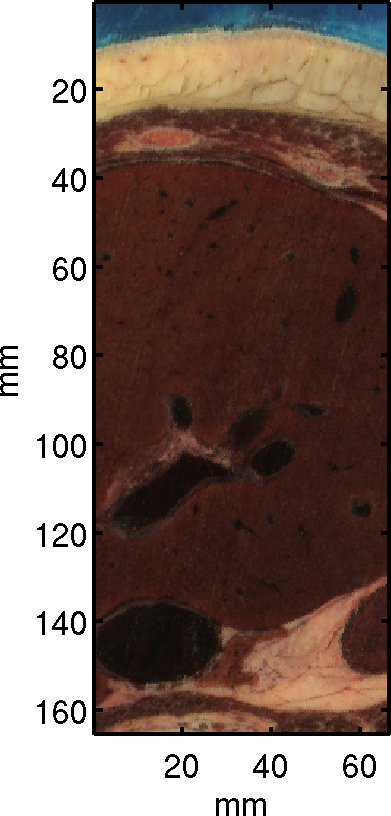
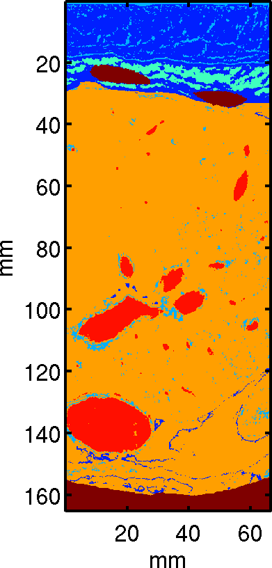
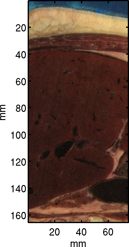
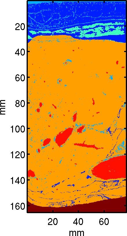
Figure 1: Digitized tissue image in RGB format orthogonal to the rib axis (top left) and along the rib axis (bottom left). The index map that tags different tissue types after flattening the maps relative to the skin surface (right).

II-B1 Define the map coordinate system

The long axis of the transducer was oriented to be parallel to the ribs. The map coordinate system was then defined with respect to this axis. The vector in between the two ribs was determined manually by first selecting points in between the ribs, then by fitting a line to them with a standard least squares regression in three dimensions. With respect to the original coordinate system, defined in the abdominal Visible Human images, the centroid is given by (564.9375, 697.2500, 325.0000) and the direction cosines of the best fit line is given by (0.6202, 0.2403, 0.7467). To complete the definition of the coordinate system an additional point in the liver was used to define the center of the image, and it was manually selected to be (350, 967, 335). In summary, the lateral imaging plane is along the transcostal line and it intersects the point in the liver. The elevation plane is orthogonal to the transcostal line and it also intersects this point. This coordinate system was used as a reference for all other calculations.

II-B2 Manually segment ribs

Since fat and bone/cartilage have a similar color on the optical images the ribs were segmented manually in each image. This segmentation data is too lengthy to reproduce here but can be provided upon request.

II-B3 Interpolation and rotation

The imaging volume was linearly interpolated (from 0.330 mm to 0.167 mm) using two successive applications of the interp2 Matlab function. Then the data set was rotated to the imaging axis coordinates. The rib segmentation coordinates underwent the same transformations.

II-B4 Flatten body surface in two dimensions using an RGB threshold detection algorithm

The body surface is curved however the ultrasound transducer is pressed into the body during imaging. To flatten the body surface relative to the transducer the superficial skin layer was detected. This body curvature was defined by the boundary between the frozen outer gelatin block and the skin surface. It was calculated with a two dimensional RGB threshold detection filter. The upper RGB threshold was (95, 160, 180) and the lower threshold was (20, 50, 65). The 2D detected surface was then filtered with a $5\times 5$ median filter. This curved surface was then used as a reference to flatten the imaging volume so that the outer skin layer was planar. This flattening can be seen by comparing the images on the left of Fig. 2 to the images on the right.

II-B5 Detect skin layer

The previous step effectively determined the superficial surface of the skin. To determine the depth of the skin layer an RGB threshold of (160, 130, 90) was used. This surface was filtered with a $20\times 20$ median filter.

II-B6 Detect fat layer and embedded connective tissue

The fat layer was detected with an RGB filter with a threshold of (160, 130, 90) for the skin/fat boundary (as described in the previous step), and a threshold of (130, 101, 56) for the fat/muscle boundary. Both detected surfaces were filtered with a $20\times 20$ median filter. Embedded within the fat layer there is a fine connective tissue. The RGB values of this connective tissue vary significantly and intersect with the surrounding fat which makes threshold detection impossible. To determine the fine structures embedded in the tissue layers a gradient based edge detection filter was used. A cube of 1.155 mm per side was convolved with the green values in the image. This convolved image was then subtracted from the original image to obtain a gradient map that can be subsequently thresholded to detect the edges. Pixels with a gradient between -3 and -30 RGB/pixel were tagged as connective tissue.

II-B7 Detect muscle layer and embedded fat

The muscle layer was detected with an RGB filter with a threshold of (99, 60, 50) for the muscle/liver boundary. Within the muscle layer the embedded fat was detected with a gradient based edge detection method on the green values using the same method described in the previous paragraph. The characteristic width of the filter was 5.115 mm and fat was detected for gradients between 0 and 50 RGB/pixel.

II-B8 Detect liver, and embedded connective tissue and blood vessels

Within the liver blood and vessels was detected for RGB values between (1, 1, 1) and (35, 30, 30). Connective tissue was detected for RGB values between (44, 26, 24) and (59, 40, 35). Fat was detected for RGB values between (102, 75, 43) and (136, 111, 95).

Once each tissue type was detected and tagged within the simulation volume, the tissue map was converted into four maps of acoustical properties: speed of sound, density, attenuation, and nonlinearity.

Their values for each tissue type are shown in Table I. In this imaging configuation the ribs were modeled to have the same acoustic impedance as bone but with the speed of sound and density reduced, instead of increased. This was done to have a larger temporal step size or equivalently CFL, which reduces the calculation time and improves the numerical accuracy. The ampltude of the reflections from bone surface were therefore accurately modeled and propagation inside the bone was considered to be irrelevant since the attenuation in bone is so large. Note that Fullwave has been used extensively to propagate ultrasound through bone [14, 11] and that this choice of an inverted impedance was motivated by optimization of the time step rather than technical difficulties of propating in bone.

Tissue	Speed	Density	Attenuation	Nonlinearity
	m/s	kg/m3	dB/MHz/cm	B/A
fat	1479	937	0.4	9.6
liver	1570	1064	0.5	7.6
muscle	1566	1070	0.15	9
connective	1613	1120	0.5	8
blood	1520	1000	0.005	5
bone	800	550	5	5

TABLE I: Tissue properties

Since the optical resolution of the visible human data set is 0.33 mm, small sub-wavelength scatterers aren’t detectable. Nevertheless these sub-resolution scatterers play an important acoustic role in the imaging physics and in particular to obtain the correct speckle statistics [17]. Sub-resolution scatterers were therefore added to the tissue maps to model the acoustical scattering properties observed in vivo. A total of 20 scatterers with a 77 $\mu$m diameter were added per resolution volume (as calculated with a 2MHz F/2 aperture). This generates fully developed speckle. The scatterers had a spatial distribution and random amplitude and with an average impedance mismatch of 2.5% relative to the background tissue. An artificial anechoic lesion was placed at the 6.5 cm focus by removing the scatterers in a spherical region within a 5 mm radius. This anechoic lesion was used to characterize the imaging properties.

The final speed of sound map for the simulation field is shown in Fig 2 in the lateral imaging plane (left), elevation plan (center), and just under the transducer suface (right). Not shown are the equivalent maps for attenuation, nonlinearity, and density which are similar in appearance. These maps include sub-resolution scatterers, which are not visible, and the negative impedance mismatch for the ribs. The location of the anechoic lesion is overlaid.

\begin{overpic}[height=203.80193pt]{figures/cmap_colorbar} \end{overpic}\begin{overpic}[width=303.53267pt]{figures/cmap_all_nocbar2} \small\put(194.0,206.0){$\leftarrow$skin} \put(194.0,180.0){$\leftarrow$fat} \put(194.0,160.0){$\leftarrow$connective} \put(194.0,150.0){$\leftarrow$muscle} \put(194.0,138.0){$\leftarrow$rib} \put(194.0,70.0){$\leftarrow$liver} \put(172.0,70.0){\color[rgb]{1,1,1}{\circle{20.0}}} \put(155.0,50.0){{\color[rgb]{1,1,1}anechoic}} \put(160.0,40.0){{\color[rgb]{1,1,1}lesion}} \put(59.0,70.0){\color[rgb]{1,1,1}{\circle{20.0}}} \put(43.0,50.0){{\color[rgb]{1,1,1}anechoic}} \put(48.0,40.0){{\color[rgb]{1,1,1}lesion}} \end{overpic}

Figure 2: The speed of sound map for the center transmit simulation field in the lateral imaging plane (left), elevation plan (center), and just under the transducer suface (right). Note the inclusion of sub-resolution scatteres and the negative impedance mismatch for the ribs. The location of the anechoic lesion is overlaid.

II-C Imaging configuration and simulation parameters

An aperture meant to represent a general transcostal imaging transdcuer was used to transmit and receive ultrasound. These transmit-receive simulation elements were placed at the skin surface of the heterogeneous acoustic tissue maps. The transducer was modeled as a 3.25 $\times$ 1.625 cm 2D array, which is consistent with the sizes typically chosen for intercostal liver imaging [18]. A a 2.5 cycle, 2 MHz, 0.2 MPa pulse focused at 65 mm was emitted without apodization. These transmit parameters are summarized in Table II. The ultrasound imaging sequence consisted of 5 transmit receive events. For each event the transducer was shifted laterally by a beamwidth calculated as 1.4 $\lambda z/d$. This shift is the equivalent of walking the aperture, or of mechanical translation. Other transmit options, such as beam steering, could have been simulated but this configuration was chosen for its simplicity. Parallel receive beamforming methods were used on the received data and they are described subsequently in sec III-D.

Transducer	Value
Parameter
Center freq.	2.0 MHz
Width	3.25 cm
Elevation	1.625 cm
Number of cycles	2.5
Tx pressure	0.2 MPa

TABLE II: Transducer parameters

The simulation was 9.3 cm deep, 3.9 cm wide, and 2.2 cm in elevation, which accomodates the footprint of the transducer with a margin to account for diffraction at the transducer edges. To generate different transmit sequence the tissue map was translated across this fixed simulation domain, which is equivalent to translating the aperture. The spatial step size was set to $\lambda/15$, calculated relative to the 2 MHz transmit center frequency. The temporal step size was set to $\Delta x/2.5c_{0}$, with $c_{0}=$ 1540 m/s, which corresponds to a Courant-Friedrichs-Lewy condition of 0.4. There were 600 million points in the spatial grid, and the evolution of the pressure field was calculated over 13,000 time steps, or equivalently 133 $\mu$s. These parameters are summarized in Table III.

Simulation	Value
Parameter
Depth (x)	9.3 cm
Lateral (y)	3.9 cm
Elevation (z)	2.2 cm
Step size ($\Delta x$)	$\lambda/15$
Step size ($\Delta t$)	$\Delta x/2.5c_{0}$
Points	$600\times 10^{6}$
Time steps	$13\times 10^{3}$

TABLE III: Simulation parameters

III Results and Discussion

III-A Characteristics of the received signal

Sound reflected from tissue structures and subresolution scatterers was measured at the grid location corresponding to the transducer surface, and then used to generate ultrasound images. A time snapshot of the simulated acoustic field is shown in Fig. 3 which overlays the pressure field on the speed of sound maps from Fig. 2. This frame corresponds to the instant in time when the transmitted pulse has reached the 65 mm focal distance. The axial section (Fig. 2, right) is taken at the transducer surface and the lateral (left) and elevation (middle) sections are taken at the center of the transducer. Given the large dynamic range, the pressure field is shown on a compressed scale so that the low pressure signal in tissue can be seen concurrently with the transmitted pulse. A movie of this transmit-receive propagation event can be found in the online resources.

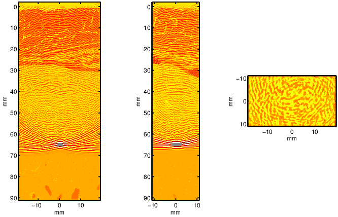
Figure 3: Snapshot in time of the pressure field on a compressed scale as it propagates through a lateral (left) elevation (middle) and axial (right) section of tissue.

The dynamic range of the acoustic signal captured by the simulation is illustrated in Fig. 4, which shows the signal measured at the center of the transducer surface as a function of time on a linear scale (left) and a dB scale (right). On the linear scale plot the 200 kPa transmitted pulse is clearly visible at at 5 $\mu$s. Following the pulse some backscattered echos are observable up to 40 $\mu$s however for larger times the echos are too small to appear on a linear scale. The right plot in Fig. 4 shows the envelope detected amplitude on a dB scale. The echo amplitude gradually decreases as a function of time until it reaches approximately -80 to -90 dB of the original transmitted amplitude. This corresponds to the numerical noise floor for the choice of points per wavelength, the CFL, and the ability of the perfectly matched layer boundaries to reduce unwanted reflections. This floor could be lowered, for example, by increasing the number of points per wavelength.

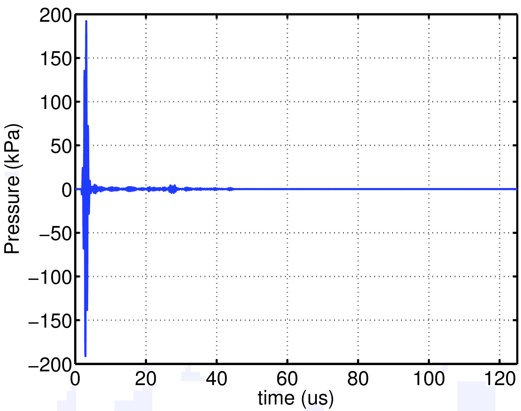
Figure 4: The pressure as a function of time measured at the center of the virtual transducer on a linear scale (left) and a dB scale (right).

Unlike a physical transducer the virtual detectors in the simulation have an almost flat frequency response which is determined by the comparatively low numerical error in the simulation. An additional filter could be implemented to model a physical transducer impulse response. The transducer was sampled at each simulated grid point in the plane, which corresponds to 201,000 elements. Since the grid size is $\lambda/15$ and the sampling frequency was set to 100 MHz this translates into 10 Gb of received data per transmit-receive event. This is a much finer spatial sampling grid than a physical array which typically has elements that vary between $\lambda/2$ and $\lambda$. Averaging over a physical element size can easily be implemented in post-processing.

The ultrasound signal measured at the transducer plane was used to determine the spatial coherence properties of the signal backscattered by the human tissue. This parameter characterizes , for example, the minimum transducer element size required to properly sample the backscattered pressure field. Note that an equivalent in vivo experiment would be difficult to implement since the physical array element size is typically below the spatial Nyquist frequency. To calculate the spatial coherence length, first the pressure as a function of time in the transducer plane was time-gated at the focal depth and a spherical focusing delay was applied (shown on the top left of Fig. 5). The pressure signal was then autocorrelated to obtain a two dimensional spatial coherence function (top left plot in Fig. 5). The lateral and elevation sections of the transducer correlation are shown on the bottom right. For this particular body wall realization the full-width half maximum (FWHM) is $1.71\lambda$ (1.32 mm) in the lateral dimension and $2.53\lambda$ (1.95 mm) and in the elevation dimension. Since the spatial coherence function is anisotropic and has a preferred orientation the global miniumum of the FWHM is at slight angle and was measured to be $1.62\lambda$ (1.24 mm). This indicates, for example, that a uniformly diced two dimensional 2 MHz transducer array designed for imaging this abdomen would ideally have a $<0.81\lambda$ ($<$0.62 mm) element size to accurately sample the spatial variations in the acoustical field.

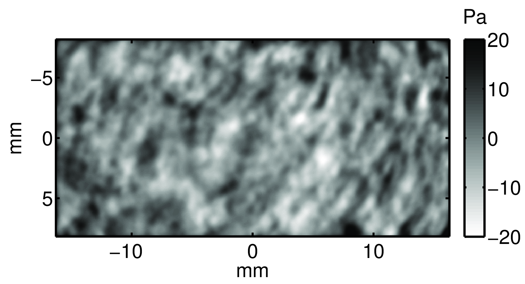
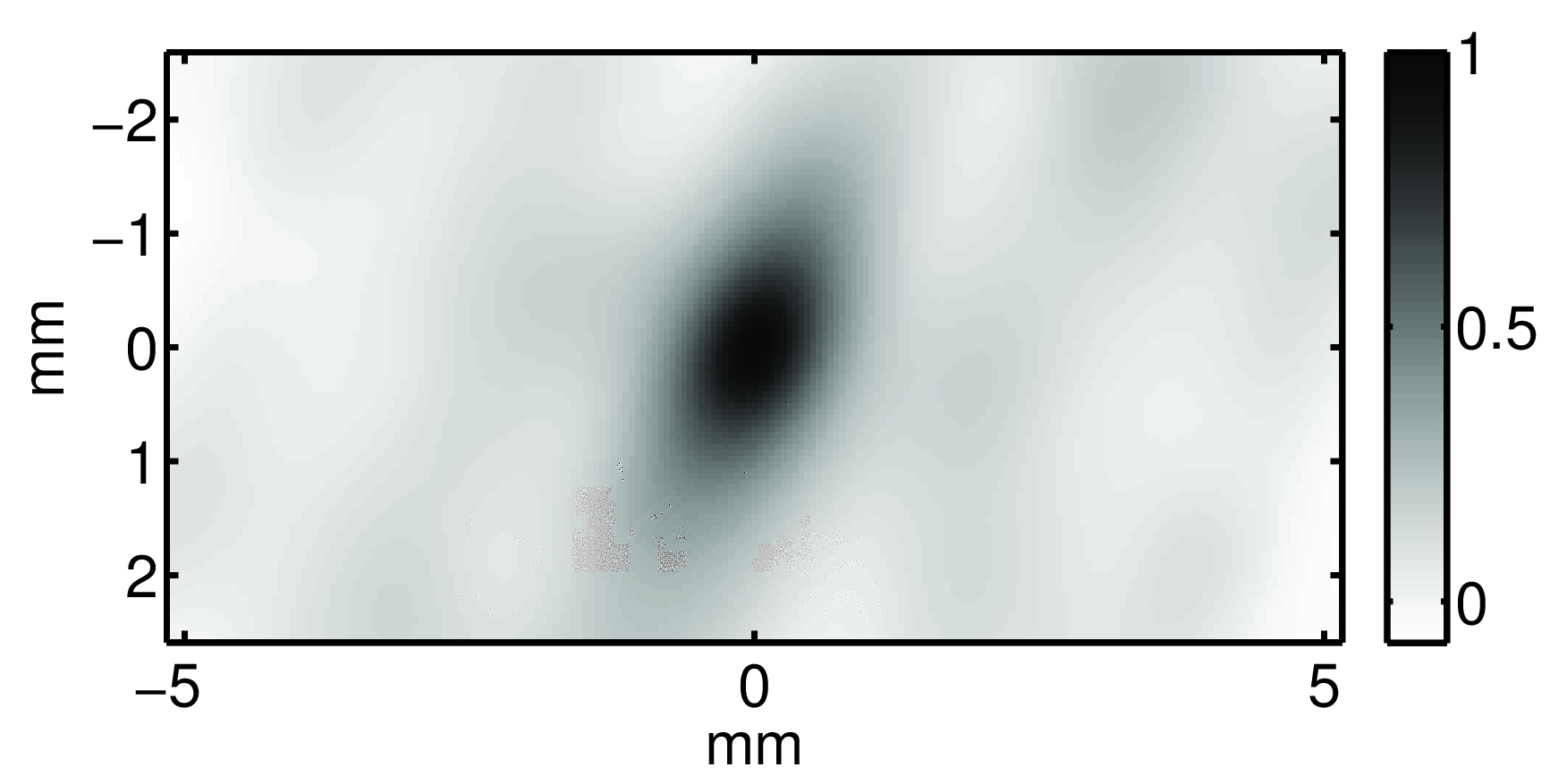
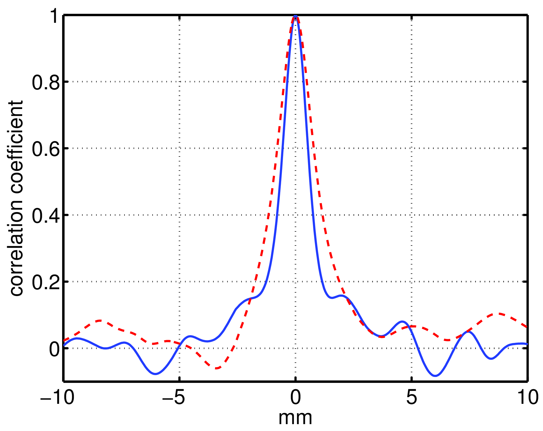
Figure 5: Signal received at the transducer surface at the focal time (top left). Spatial coherence as determined by the auto-correlation of the signal received at the transducer surface (top right) and the corresponding lateral (solid line) and elevation (dashed line) sections of the spatial coherence function (bottom).

III-B Fundamental and harmonic beams within the body

One of the advantages of simulations compared to experiments is that the acoustic field can be estimated in locations where it would not be possible to scan with a hydrophone. The acoustic field within the human body, for example, can provide valuable information on the beamforming characteristics of the ultrasound array. Some general observations on the beams are made here and a more detailed analysis on the influence of the beam properties on image quality is given in Part 2 of this paper.

To investigate the beams at the fundamental and harmonic frequencies the pressure field was integrated in time for all points in the three dimensional simulation domain yielding the intensity (shown in Fig. 6). The focal gain is apparent in the lateral beams (on the left of Fig. 6) and the ribs are visible in the elevation beams (on the right of Fig. 6) as areas of low intensity at 30 and 35 mm depth. The beam splits into two parts in the lateral dimension and it deviates significantly from the geometric propagation axis, especially in the elevation dimension.

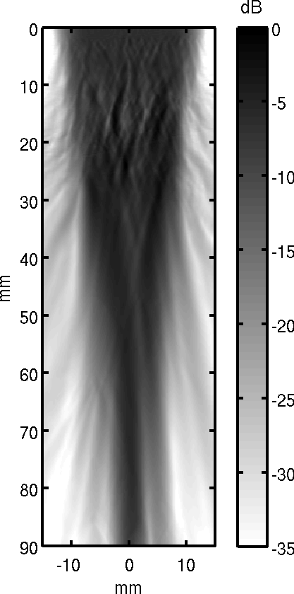
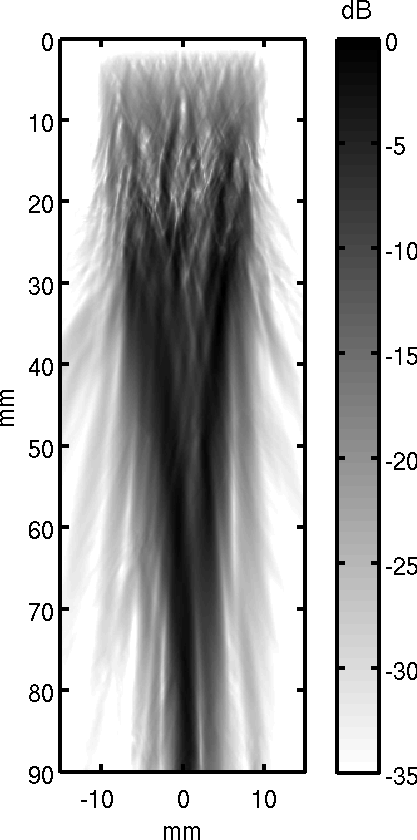
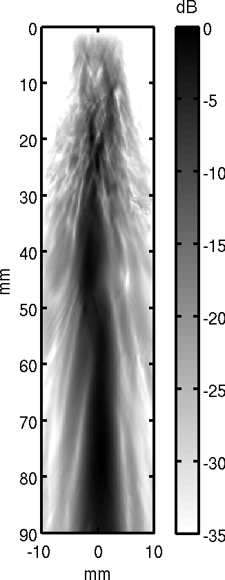
Figure 6: The intensity in the lateral plane and elevation planes for the fundamental frequency (top) and the harmonic frequency (bottom). The harmonic beam appears to be fully developed at approximately 20 mm of depth, which is before the ribs (cf. Fig. 2).

A quantitative comparison between the different beams is shown in Fig. 7 which plots the lateral and elevation beamplots at the 65 mm focal depth. Even though the transducer has a 2:1 aspect ratio the width of the lateral and elevation beams at the focus are very similar. This is due to the tissue inhomogeneities which significantly alter the beam shape throughout its propagation path (Fig. 6). The harmonic beamplots are narrower than the fundamental beamplots probably due to a self-focusing effect. Based on the beamplots alone one would therefore hypothesize that the harmonic images to be better than the fundamental images. This will be investigated briefly in Sec. III-D and more thoroughly in Part II of this paper. Before establishing this link to image quality, the aberration is described and quantified.

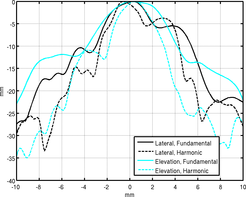
Figure 7: Beamplots at the focus (65 mm depth) for the beams shown in Fig. 6. The harmonic beamplots are slightly narrower due to the self-focusing effect. However there isn’t a significant difference between lateral and elevation beamwidth.

III-C Aberration after the ribs

Phase aberration measures the deviation of a beam from a predetermined phase profile, such as the ideal focusing profile in a homogeneous medium. In a heterogeneous medium, or distributed aberrator, such as the human body, the phase aberration changes as the wave propagates. Since, in this simulation, the pressure field is known throughout the body, the phase aberration can be calculated at different depths.

Here the the pressure was measured in the lateral and elevation dimensions at a depth of 35 mm, just after the ribs. The aberration calculation therefore includes the influence of the near field skin, connective tissue, fat, and muscle, which are strong aberrators compared to the relatively homogeneous liver because there is a large impedance mismatch between different tissue types. To determine the aberration of the field an inverse spherical delay, representing the ideal homogeneous medium phase, was applied to the signals. A plot of this field in the lateral axis is shown in Fig. 8. The remaining phase, i.e. any phase component that isn’t constant perpendicular to the propagation axis, represents the phase error, or phase aberration from the ideal focusing delay.

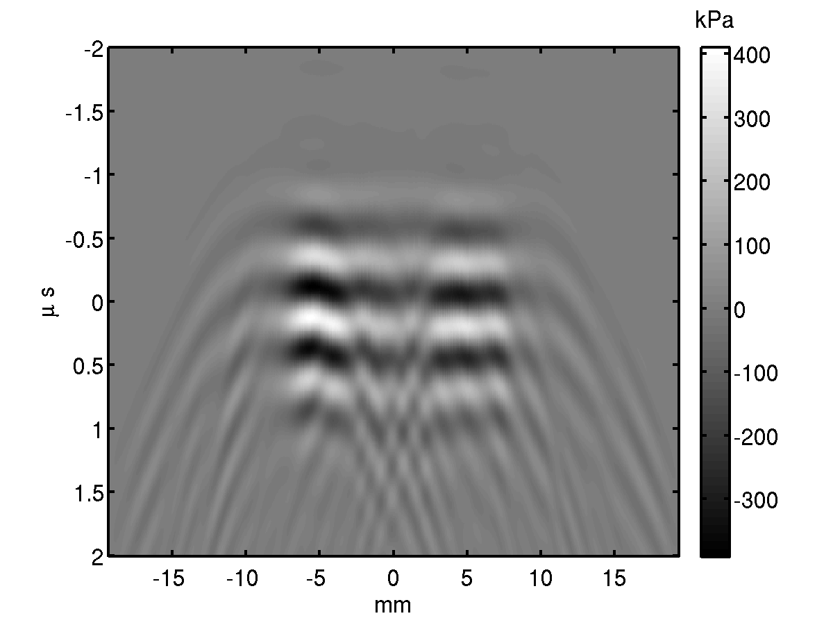
Figure 8: Received pressure in the lateral axis measured at 3.5 cm depth (just after the ribs) at the fundamental frequency (left) and harmonic frequency (right). A spherical delay was applied to the signals to correct for the focusing profile.

The signal was interpolated by a factor of three and then discrete normalized cross correlation was used to establish discrete estimates of the time delays. These discrete estimates were then fitted to a parabola to determine the continuous delay estimates [19].

	Fundamental	Harmonic
lateral	23.4 ns	16.2 ns
elevation	23.5 ns	12.5 ns

TABLE IV: RMS phase aberration at 3.5 cm depth in the lateral and elevation dimensions

One of the challenges in calculating the phase aberration comes from areas of diffraction at the beam edges. In these edge diffraction regions there is significant aberration but very little energy compared to the central part of the pulse. This is clearly visible in Fig. 8 where the low energy diffraction edges of the pulse, beyond $\pm 7$ mm, have deviated significantly from a planar profile. However these low-energy areas are not particularly relevant to tissue-generated phase aberration in an imaging context. A simple threshold was therefore used to eliminate the aberration estimates where the intensity was less than 10% of the maximum. Values above this threshold were used to determine the root-mean-square (RMS) aberrations. At the fundamental frequency this aberration is 23.4 ns laterally and 23.5 ns in elevation. In an ex vivo experiment Hinkelman et al. [20] determined the deviation of the arrival time across a mechanically scanned 2-D aperture for ultrasound propagating through a human chest wall. These root-mean-square estimates were, on average, 21.3 ns.

The aberration at the second harmonic frequency is small by slightly less than a factor of two, 16.2 ns laterally and 12.5 ns in elevation. These values are summarized in Table IV.

III-D Image analysis

Conventional B-mode images were generated in silico using the same propagation-based imaging physics used by an ultrasound scanner. The 2 MHz pulse was transmitted into the Visible Human acoustical maps (as described previously in Sec II-C), then the backscattered signal was received at the transducer location (as described previously in Sec III-A), and finally conventional delay and sum beamforming was performed to generate B-mode images.

Beamforming for the two dimensional array was performed in the lateral and elevation dimensions, across all 201,000 simulation points in the transducer plane. I.e. each grid point acted as a transducer element. Since the simulation elements are significantly smaller than transducer elements the signal could also have been averaged over the footprint of a single transducer element. Furthermore, data within the kerf footprint could have been ignored to model a more precise angular response. However these operations did not make a significant difference in subsequently presented comparative image quality analysis and were therefore not performed here.

Dynamic receive focusing was performed in both lateral and elevation dimensions. A minimum F/# value of 3 was used to maintain a uniform speckle pattern. Parallel receive beamforming was used to generate A-lines across half of a beamwidth (i.e. $1.4\lambda z/2D$). This reduced the number of transmit-receive events necessary to generate a B-mode image to a total of five each with a processing time of 10 hours on a 96 CPU computer cluster. The fundamental and harmonic compenents of the backscattered signal were calulculated by filtering, respectively, at the transmit or at two times the transmit frequency using a standard Gaussian filter.

The resulting fundamental and harmonic B-mode images (Fig. 9) clearly show an anechoic lesion that is visible at the 65 mm focus. The speed of sound map corresponding to the image location is shown for reference on the left of Fig. 9 with the position of the anechoic region lesion outlined at the focus. As might be expected the contrast to noise ratio (CNR), which quantifies the lesion detectability, is higher for the harmonic image (CNR=0.79) than the fundamental image (CNR=0.67). Features that are observable in the speed of sound map are also visible in the B-mode images. For example the near field tissue layers between 0 and 30 mm appear bright and the tissue structures within the liver at 48 mm, and 60 mm depth are visible.

\begin{overpic}[width=108.405pt]{figures/cmap_lat_liver_new_2MHz_10} \put(71.0,94.0){\bf{\color[rgb]{1,1,1}\circle{21.0}}} \put(55.0,60.0){\color[rgb]{1,1,1}\line(0,1){165.0}} \put(87.0,60.0){\color[rgb]{1,1,1}\line(0,1){165.0}} \put(55.0,60.0){\color[rgb]{1,1,1}\line(1,0){32.0}} \put(55.0,225.0){\color[rgb]{1,1,1}\line(1,0){32.0}} \put(55.0,72.0){\small\bf{\color[rgb]{1,1,1} anechoic }} \put(61.0,63.0){\small\bf{\color[rgb]{1,1,1} lesion }} \end{overpic} \begin{overpic}[width=54.2025pt]{figures/bmode_fund_liver_new_2MHz_10} \put(16.0,55.0){{\color[rgb]{1,1,1}0.67}} \put(5.0,180.0){\scriptsize{\color[rgb]{0,0,0} Fundamental }} \end{overpic} \begin{overpic}[width=54.2025pt]{figures/bmode_harm_liver_new_2MHz_10} \put(16.0,55.0){{\color[rgb]{1,1,1}0.79}} \put(7.0,180.0){\scriptsize{\color[rgb]{0,0,0} Harmonic }} \end{overpic}

Figure 9: Harmonic frequency B-mode images calculated with a (from left to right) 1D transducer with ribs, 2D transducer without ribs, and a 2D transducer with ribs. The corresponding speed of sound map is shown on the right.

IV Summary and conclusion

In summary the we have described how the optical data from the Visible Human project can be used to generate anatomically realistic maps of the acoustical properties human tissue for an intercostal imaging scenario. A divide and conquer approach that segmented different regions and then detected specific tissue types within those regions was used. These optical image to acoustical map transformation techniques are applicable to other areas of the body. The acoustical maps can be used to simulate ultrasound imaging, therapeuetic, or generally any acoustic emission. Here the Fullwave simulation tool was used to generate highly realistic harmonic and fundamental B-mode images based on the first principles of propagation and reflection. Since the acoustical field is known throughout the simulation domain measurements of the beamplot, phase aberration, and spatial coherence were also calculated. It was shown that the fundamental and harmonic beamplots have a similar width, sidelobe level, and aberration profiles. In the companion paper the acoustical maps and image characterization tools established here are used to determine the influence of clutter in this intercostal imaging scenario. In conclusion, with these simulations we have generated the first three dimensional, ultrasound images based on propagation physics through a highly realistic anatomical model of the human body.

References

- [1] J. A. Jensen, “Field: A program for simulating ultrasound systems,” Med. Biol. Eng. Comp., col. 10th Nordic-Baltic Conference on Biomedical Imaging, vol. 4, no. 1, pp. 351–353, 1996.
- [2] T. Christopher and K. Parker, “New approaches to nonlinear diffractive field propagation,” J. Acoust. Soc. Am., vol. 90, pp. 488–499, 1991.
- [3] R. J. Zemp, J. Tavakkoli, and R. Cobbold, “Modeling of nonlinear ultrasound propagation in tissue from array transducers,” J. Acoust. Soc. Am., vol. 113, no. 1, pp. 139–152, Jan 2003.
- [4] F. Dagrau, M. Rénier, R. Marchiano, and F. Coulouvrat, “Acoustic shock wave propagation in a heterogeneous medium: A numerical simulation beyond the parabolic approximation,” The Journal of the Acoustical Society of America, vol. 130, no. 1, pp. 20–32, 2011.
- [5] P. Yuldashev and V. Khokhlova, “Simulation of three-dimensional nonlinear fields of ultrasound therapeutic arrays,” Acoustical physics, vol. 57, no. 3, pp. 334–343, 2011.
- [6] T. D. Mast, L. M. Hinkelman, M. J. Orr, V. W. Sparrow, and R. C. Waag, “Simulation of ultrasonic pulse propagation through the abdominal wall,” Journal of the Acoustical Society of America, vol. 102, no. 2, pp. 1177–1190, Aug 1997.
- [7] T. D. Mast, “Two- and three-dimensional simulations of ultrasonic propagation through human breast tissue,” Acoustics Research Letters Online, vol. 3, no. 2, pp. 53–58, 2002.
- [8] B. E. Treeby and B. T. Cox, “k-wave: Matlab toolbox for the simulation and reconstruction of photoacoustic wave fields,” Journal of biomedical optics, vol. 15, no. 2, pp. 021 314–021 314, 2010.
- [9] G. Pinton, J. Dahl, S. Rosenzweig, and G. Trahey, “A heterogeneous nonlinear attenuating full-wave model of ultrasound,” Ultrasonics, Ferroelectrics and Frequency Control, IEEE Transactions on, vol. 56, no. 3, pp. 474–488, 2009.
- [10] G. Pinton, J. Dahl, and G. Trahey, “Sources of image degradation in fundamental and harmonic ultrasound imaging: A nonlinear, full-wave, simulation study,” IEEE Trans. Ultrason. Ferroelectr. Freq. Control, 2011.
- [11] G. Pinton, J. Aubry, M. Fink, and M. Tanter, “Effects of nonlinear ultrasound propagation on high intensity brain therapy,” Medical physics, vol. 38, no. 3, p. 1207, 2011.
- [12] G. Pinton, G. Trahey, and J. Dahl, “Spatial coherence in human tissue: implications for imaging and measurement,” Ultrasonics, Ferroelectrics, and Frequency Control, IEEE Transactions on, vol. 61, no. 12, pp. 1976–1987, 2014.
- [13] M. Jakovljevic, G. F. Pinton, J. J. Dahl, and G. E. Trahey, “Blocked elements in 1-d and 2-d arrays—part i: Detection and basic compensation on simulated and in vivo targets,” IEEE Transactions on Ultrasonics, Ferroelectrics, and Frequency Control, vol. 64, no. 6, pp. 910–921, 2017.
- [14] G. Pinton, J.-F. Aubry, M. Fink, and M. Tanter, “Numerical prediction of frequency dependent 3d maps of mechanical index thresholds in ultrasonic brain therapy,” Medical Physics, p. 299, 2011.
- [15] V. Spitzer, M. Ackerman, A. Scherzinger, and D. Whitlock, “The visible human male: a technical report,” Journal of the American Medical Informatics Association, vol. 3, no. 2, pp. 118–130, 1996.
- [16] G. Pinton, J. Dahl, S. Rosenzweig, and G. Trahey, “A heterogeneous nonlinear attenuating full-wave model of ultrasound,” IEEE Trans. Ultrason., Ferroelec., Freq. Contr., vol. 56, no. 3, pp. 474–88, Mar 2009.
- [17] R. F. Wagner, S. W. Smith, J. M. Sandrik, and H. Lopez, “Statistics of speckle in ultrasound b-scans,” Sonics and Ultrasonics, IEEE Transactions on, vol. 30, no. 3, pp. 156–163, 1983.
- [18] T. L. Szabo and P. A. Lewin, “Ultrasound transducer selection in clinical imaging practice,” Journal of Ultrasound in Medicine, vol. 32, no. 4, pp. 573–582, 2013.
- [19] G. F. Pinton, J. J. Dahl, and G. E. Trahey, “Rapid tracking of small displacements with ultrasound,” IEEE transactions on ultrasonics, ferroelectrics, and frequency control, vol. 53, no. 6, pp. 1103–1117, 2006.
- [20] L. M. Hinkelman, T. L. Szabo, and R. C. Waag, “Measurements of ultrasonic pulse distortion produced by human chest wall,” The Journal of the Acoustical Society of America, vol. 101, no. 4, pp. 2365–2373, 1997.