The inverse problem for Hamilton-Jacobi equations and semiconcave envelopes

Abstract.

We study the inverse problem, or inverse design problem, for a time-evolution Hamilton-Jacobi equation. More precisely, given a target function $u_{T}$ and a time horizon $T>0$, we aim to construct all the initial conditions for which the viscosity solution coincides with $u_{T}$ at time $T$. As it is common in this kind of nonlinear equations, the target might not be reachable. We first study the existence of at least one initial condition leading the system to the given target. The natural candidate, which indeed allows determining the reachability of $u_{T}$, is the one obtained by reversing the direction of time in the equation, considering $u_{T}$ as terminal condition. In this case, we use the notion of backward viscosity solution, that provides existence and uniqueness for the terminal-value problem. We also give an equivalent reachability condition based on a differential inequality, that relates the reachability of the target with its semiconcavity properties. Then, for the case when $u_{T}$ is reachable, we construct the set of all initial conditions for which the solution coincides with $u_{T}$ at time $T$. Note that in general, such initial conditions are not unique. Finally, for the case when the target $u_{T}$ is not necessarily reachable, we study the projection of $u_{T}$ on the set of reachable targets, obtained by solving the problem backward and then forward in time. This projection is then identified with the solution of a fully nonlinear obstacle problem, and can be interpreted as the semiconcave envelope of $u_{T}$, i.e. the smallest reachable target bounded from below by $u_{T}$.

1. Introduction

We consider the initial-value problem for a Hamilton-Jacobi equation of the form

(1.1) $$\left\{\begin{array}[]{ll}\partial_{t}u+H(D_{x}u)=0,&\text{in}\ [0,T]\times\mathbb{R}^{n},\\ \vskip 4.2679pt\cr u(0,x)=u_{0}(x),&\text{in}\ \mathbb{R}^{n},\end{array}\right.$$

where $u_{0}\in\operatorname{Lip}(\mathbb{R}^{n})$ and the Hamiltonian $H:\mathbb{R}^{n}\rightarrow\mathbb{R}$ is assumed to satisfy the following hypotheses:

(1.2) $$H\in C^{2}(\mathbb{R}^{n}),\quad H_{pp}(p)>0,\ \forall p\in\mathbb{R}^{n},\quad\text{and}\quad\lim_{|p|\to\infty}\dfrac{H(p)}{|p|}=+\infty.$$

Here, the unknown $u$ is a function $[0,T]\times\mathbb{R}^{n}\longrightarrow\mathbb{R}$, the notation $\partial_{t}u$ stands for the derivative of $u$ with respect to the first variable and $D_{x}u$, for the vector of partial derivatives with respect to the second group of variables. The inequality $H_{pp}(p)>0$ in (1.2) means that the Hessian matrix of $H$ at $p$ is positive definite. The study of equations such as (1.1) arises in the context of optimal control theory and calculus of variations, where the value function satisfies, in a weak sense, a Hamilton-Jacobi equation like (1.1) (see [4, 7, 8, 13, 19, 20] and the references therein). In this context, Hamilton-Jacobi equations have applications in a wide range of fields such as economics, physics, mathematical finance, traffic flow and geometrical optics.

It is well known that, due to the presence of a nonlinear term in the equation, one cannot in general expect the existence of a classical $C^{1}$ solution for problem (1.1), even if the initial datum $u_{0}$ is assumed to be very smooth. On the other hand, continuous solutions satisfying the equation almost everywhere might not be unique. In the early 80’s, Crandall and Lions solved this problem in [18] by introducing the notion of viscosity solution (Definition 4.1), see also [7, 13, 17, 22].

For any initial condition $u_{0}\in\operatorname{Lip}(\mathbb{R}^{n})$, existence and uniqueness of a viscosity solution $u\in\operatorname{Lip}([0,T]\times\mathbb{R}^{n})$ was established in [18]. This solution can be obtained, using the method of the vanishing viscosity (see [17, 18, 25]), as the limit when $\varepsilon\to 0^{+}$ of the unique solution of the parabolic problem

$$\left\{\begin{array}[]{ll}\partial_{t}u-\varepsilon\,\Delta_{x}u+H(D_{x}u)=0,&\text{in}\ [0,T]\times\mathbb{R}^{n},\\ \vspace{1.5mm}\cr u(0,x)=u_{0}(x),&\text{in}\ \mathbb{R}^{n},\end{array}\right.$$

for which, by the standard theory of nonlinear parabolic equations, existence and uniqueness of a classical solution holds as long as $\varepsilon>0$.

In view of the existence and uniqueness of a viscosity solution for problem (1.1), we can define, for a fixed $T>0$, the following nonlinear operator, which associates to any initial condition $u_{0}$, the function $u(T,\cdot)$, where $u$ is the viscosity solution of (1.1):

$$\begin{array}[]{cccl}S^{+}_{T}:&\operatorname{Lip}(\mathbb{R}^{n})&\longrightarrow&\operatorname{Lip}(\mathbb{R}^{n})\\ &u_{0}&\longmapsto&S^{+}_{T}u_{0}:=u(T,\cdot)\end{array}$$

Our goal in this work is to study the inverse problem associated to (1.1). More precisely, for a given target function $u_{T}$ and a time horizon $T>0$, we want to construct all the initial conditions $u_{0}$ such that the viscosity solution of (1.1) coincides with $u_{T}$ at time $T$. This type of problems, also known in the literature as data assimilation problems, have relevant importance in any kind of evolution models. For instance in meteorology [21, 27], where the climate prediction must take into account not only the observations at the present time, but also at past times. For related results in the context of Hamilton-Jacobi equations, we refer to [15, 16, 26] and the references therein.

The first thing one notices when addressing this problem is that not all the Lipschitz targets are reachable. Indeed, as it is well known, the viscosity solution to (1.1) is always a semiconcave function (Definition 4.3). Therefore, an obvious necessary (but not sufficient) condition for the reachability of $u_{T}$ is that it must be a semiconcave function. We then split the problem in the following three steps:

1. First, we study the reachability of the target, i.e. the existence of at least one $u_{0}$ satisfying $S_{T}^{+}u_{0}=u_{T}$. The natural candidate is the one obtained by reversing the direction of time in the equation (1.1), considering the target $u_{T}$ as terminal condition (see the definition of backward viscosity solution in Definition 4.2). Indeed, it turns out that the initial datum recovered by this method, allows one to determine whether the target is reachable or not (see Theorem 2.1). We also obtain a reachability criterion based on a differential inequality (see Theorem 2.2), that links the reachability of the target with its semiconcavity properties.

2. Secondly, if the target is reachable, we construct all the initial conditions $u_{0}$ such that $S_{T}^{+}u_{0}=u_{T}$ (see Theorem 2.3). As we will see, such $u_{0}$ is not in general unique. The impossibility of uniquely determining the initial condition from the solution at time $T$ is a main feature in first-order nonlinear evolution equations like (1.1), and can be interpreted as a loss of the initial information due to the nonlinear effects and the loss of regularity.

3. Finally, if the target $u_{T}$ is not reachable, we project it on the set of reachable targets by solving the problem (1.1) backward in time and then forward. As we will see, this projection has some interesting properties and seems to be the most natural one. For instance, it is the smallest reachable target which is bounded from below by $u_{T}$ and can be characterized as the viscosity solution of a fully nonlinear obstacle problem (see Theorem 2.5).

The idea of iterating forward and backward resolutions of the model in order to reconstruct previous states has already been exploited in different types of evolution equations, and seems to be an effective method to deal with data assimilation problems like the one treated in this paper. See for example the works [2, 3] where a Back and Forth Nudging algorithm is proposed.

The paper is structured as follows: in Section 2, we present and discuss our main results concerning each one of the three points described above. Section 3 is devoted to some examples that illustrate these results. In Section 4, we introduce the notion of backward viscosity solution, present some of its well-known properties, and then we prove the reachability criterion of Theorem 2.1. In Section 5, we give the proof of the results about the construction of initial conditions for a reachable target, Theorems 2.3 and 2.4. Section 6 is devoted to the study of the composition operator $S_{T}^{+}\circ S_{T}^{-}$, that can be viewed as a projection of $u_{T}$ on the set of reachable targets. In this section we prove Theorem 2.5, that identifies the image of $S_{T}^{+}\circ S_{T}^{-}$ with the viscosity solution of a fully nonlinear obstacle problem. Then, we discuss the connection of this obstacle problem with the concave envelope of a function and give a geometrical interpretation of $S_{T}^{+}(S_{T}^{-}u_{T})$ as the semiconcave envelope of $u_{T}$. We end the Section 6 with the proof of Theorem 2.2, that gives a criterion for the reachability of a target in terms of a differential inequality. Finally, in Section 7 we discuss the contributions of this work and present some possible extensions and future perspectives.

2. Main results

2.1. Reachability criteria

For a given target $u_{T}\in\operatorname{Lip}(\mathbb{R}^{n})$, our first goal is to determine whether or not there exists at least one initial condition $u_{0}$ such that $S_{T}^{+}u_{0}=u_{T}$. That is, we want to give a necessary and sufficient condition for the set

(2.1) $$I_{T}(u_{T}):=\left\{u_{0}\in\operatorname{Lip}(\mathbb{R}^{n})\,;\ S_{T}^{+}u_{0}=u_{T}\right\}$$

to be nonempty. In Theorem 2.1 below, for any $u_{T}\in\operatorname{Lip}(\mathbb{R}^{n})$, we give a reachability condition based on the so-called backward viscosity solution (see Definition 4.2). This notion of solution was already used in [9] in order to study the relation between the regularity of solutions and the time-reversibility of problem (1.1).

It is well known (see Section 4 for more details) that in the class of backward viscosity solutions, existence and uniqueness holds for the terminal-value problem

(2.2) $$\left\{\begin{array}[]{ll}\partial_{t}w+H(D_{x}w)=0,&\text{in}\ [0,T]\times\mathbb{R}^{n},\\ \vskip 4.2679pt\cr w(T,x)=u_{T}(x),&\text{in}\ \mathbb{R}^{n}.\end{array}\right.$$

Actually, analogously to the (forward) viscosity solutions, the backward viscosity solution can be obtained as the limit when $\varepsilon\to 0^{+}$ of the solution to the problem

$$\left\{\begin{array}[]{ll}\partial_{t}w+\varepsilon\,\Delta_{x}w+H(D_{x}w)=0,&\text{in}\ [0,T]\times\mathbb{R}^{n},\\ \vspace{1.5mm}\cr w(T,x)=u_{T}(x),&\text{in}\ \mathbb{R}^{n}.\end{array}\right.$$

Hence, we can define the nonlinear operator

$$\begin{array}[]{cccl}S^{-}_{T}:&\operatorname{Lip}(\mathbb{R}^{n})&\longrightarrow&\operatorname{Lip}(\mathbb{R}^{n})\\ &u_{T}&\longmapsto&S^{-}_{T}u_{T}:=w(0,\cdot)\end{array}$$

which associates to any terminal condition $u_{T}$, the function $w(0,\cdot)$, i.e. the unique backward viscosity solution of (2.2) at time $0$.

Here we state the first reachability criterion, which identifies the reachable targets with the fix-points of the composition operator $S_{T}^{+}\circ S_{T}^{-}$.

Theorem 2.1.

Let $H$ satisfy (1.2), $u_{T}\in\operatorname{Lip}(\mathbb{R}^{n})$ and $T>0$. Then, the set $I_{T}(u_{T})$ defined in (2.1) is nonempty if and only if $S_{T}^{+}\left(S_{T}^{-}u_{T}\right)=u_{T}.$

Reversing the time in the equation in order to find initial conditions conducting to a given target is a natural approach in all kinds of evolution equations. However, in many cases, the obtained initial condition does not lead the system back to the target. In the case of the problem (1.1), Theorem 2.1 ensures that the target is reachable if and only if this technique of reversing the time gives the desired initial condition.

As a drawback of this result, we need to solve first the problem (2.2) and then the problem (1.1) in order to determine if a target is reachable or not. Next, for the one-dimensional case, and for the case of a quadratic Hamiltonian in any space-dimension, i.e.

(2.3) $$H(p)=\dfrac{\langle A\,p,p\rangle}{2}\quad\text{where $A$ is a definite positive $n\times n$ matrix},$$

we give a reachability criterion based on a differential inequality.

Theorem 2.2.

Let $u_{T}\in\operatorname{Lip}(\mathbb{R}^{n})$ and $T>0$.

1. If $H$ satisfies (1.2) and the space-dimension is $1$, the set $I_{T}(u_{T})$ defined in (2.1) is nonempty if and only if $u_{T}$ satisfies the inequality

   $$\partial_{xx}u_{T}-\left(T\,H_{pp}(\partial_{x}u_{T})\right)^{-1}\leq 0,\qquad\text{in}\ \mathbb{R}$$

   in the viscosity sense (see Definition 6.2).

2. If $H$ is given by (2.3), the set $I_{T}(u_{T})$ defined in (2.1) is nonempty if and only if $u_{T}$ satisfies the inequality

   $$\lambda_{n}\left[D^{2}u_{T}-\dfrac{A^{-1}}{T}\right]\leq 0,\qquad\text{in}\ \mathbb{R}^{n}$$

   in the viscosity sense (see Definition 6.2).

Here, $D^{2}u_{T}$ denotes the Hessian matrix of $u_{T}$, and the expression $\lambda_{n}[X]$ denotes the largest eigenvalue of the $n\times n$ symmetric matrix $X$. Analogously, we will use $\lambda_{1}[X]$ to denote the smallest eigenvalue of $X$.

Remark 2.1.

In the multidimensional case, Theorem 2.2 only applies to quadratic Hamiltonians. This is due to the fact that for this case, the Hessian matrix of $H$ is constant over $\mathbb{R}^{n}$. In the one-dimensional case, the result can be generalized to any strictly convex $H$, however, the arguments that we use in the proof do not apply to higher dimensions, and a similar necessary and sufficient reachability condition do not seem to be straightforward for the case of a general convex Hamiltonian in any space-dimension (see Remark 6.1).

Note in addition that, in the one-dimensional case, the transformation

(2.4) $$v(t,x)\longmapsto f^{\prime}(v(t,x))$$

allows to reduce the study of any scalar conservation law of the form

$$\partial_{t}v+\partial_{x}(f(v))=0,$$

to the case of Burgers equation (see for example [24])

$$\partial_{t}w+\partial_{x}\left(\dfrac{w^{2}}{2}\right)=0.$$

Then, using the relation between Hamilton-Jacobi equations and scalar conservations laws (see for example [16]), in one-space dimension we can reduce the study of (1.1) to the case $H(p)=\dfrac{p^{2}}{2}$.

Observe that the reachability criterion of Theorem 2.2 does not involve the operators $S_{T}^{+}$ and $S_{T}^{-}$. Furthermore, this result relates the reachability of a target $u_{T}$ with its semiconcavity properties. We recall that a continuous function $f:\mathbb{R}^{n}\to\mathbb{R}$ is concave if and only if it is a viscosity solution of $\lambda_{n}[D^{2}f]\leq 0$ (see for example the work of Oberman [28]). In view of this, from Theorem 2.2 and the properties of semiconcave functions in Proposition 4.3 below, we can deduce the following result, that relates the reachability of a function $u_{T}$ with its semiconcavity constant.

Corollary 2.1.

Let $H$ be given by (2.3), $u_{T}\in\operatorname{Lip}(\mathbb{R}^{n})$ and $T>0$.

1. If $I_{T}(u_{T})\neq\emptyset$, then $u_{T}$ is semiconcave with linear modulus and constant $\dfrac{1}{T\lambda_{1}(A)}$.

2. If $u_{T}$ is semiconcave with linear modulus and constant $\dfrac{1}{T\lambda_{n}(A)}$, then $I_{T}(u_{T})\neq\emptyset$.

See a detailed proof of this corollary in Section 6. For the precise definition of semiconcave function with linear modulus, see Definition 4.3.

Remark 2.2.

1. Observe that, in the particular case of a Hamiltonian given by (2.3) with $A=c\,I_{n}$ and $c>0$, i.e.

   $$H(p)=c\dfrac{|p|^{2}}{2},$$

   we have $\lambda_{1}(A)=\lambda_{n}(A)=c$. Then, Corollary 2.1 implies that $I_{T}(u_{T})\neq\emptyset$ if and only if $u_{T}$ is semiconcave with linear modulus and constant $\dfrac{1}{c\,T}$.

2. It can be easily checked that, if a function $u_{T}$ satisfies the inequality of Theorem 2.2 for some $T>0$, then the same inequality holds for any $T^{\prime}\in]0,T]$. This implies that the set of reachable targets becomes smaller as we increase the time horizon $T$. In the limit case, if we let $T$ go to $\infty$, we observe that only the concave functions are reachable for all $T>0$.

2.2. Initial data construction

Here, for the case when the target $u_{T}$ is reachable, our goal is to construct all the initial conditions $u_{0}$ in $I_{T}(u_{T})$. Our construction relies on the fact that, in view of Theorem 2.1, $I_{T}(u_{T})\neq\emptyset$ implies that $S_{T}^{-}u_{T}\in I_{T}(u_{T})$.

Theorem 2.3.

Let $H$ satisfy (1.2) and $T>0$. Let $u_{T}\in\operatorname{Lip}(\mathbb{R}^{n})$ be such that $I_{T}(u_{T})\neq\emptyset$ and set the function $\tilde{u}_{0}:=S_{T}^{-}u_{T}$. Then, for any $u_{0}\in\operatorname{Lip}(\mathbb{R}^{n})$, the two following statements are equivalent:

1. $u_{0}\in I_{T}(u_{T})$;

2. $u_{0}(x)\geq\tilde{u}_{0}(x),\ \forall x\in\mathbb{R}^{n}\quad\text{and}\quad u_{0}(x)=\tilde{u}_{0}(x),\ \forall x\in X_{T}(u_{T}),$

where $X_{T}(u_{T})$ is the subset of $\mathbb{R}^{n}$ given by

$$X_{T}(u_{T}):=\left\{z-T\,H_{p}(\nabla u_{T}(z));\ \forall z\in\mathbb{R}^{n}\ \text{such that}\ u_{T}(\cdot)\ \text{is differentiable at}\ z\right\}.$$

See the Examples 1 and 2 for an illustration of this result. In view of Theorem 2.3, when it is nonempty, the set of initial conditions $I_{T}(u_{T})$ defined in (2.1) can be given in the following way:

$$I_{T}(u_{T})=\left\{\tilde{u}_{0}+\varphi\,;\,\varphi\in\operatorname{Lip}(\mathbb{R}^{n})\ \text{such that}\ \varphi\geq 0\ \text{and}\ \text{supp}(\varphi)\subset\mathbb{R}^{n}\setminus X_{T}(u_{T})\right\}.$$

All the functions in $I_{T}(u_{T})$ coincide with $\tilde{u}_{0}$ in the set $X_{T}(u_{T})\subset\mathbb{R}^{n}$, while in its complement, they are bigger or equal than $\tilde{u}_{0}$. We can also write

$$I_{T}(u_{T})=\tilde{u}_{0}+\mathcal{L}(\mathbb{R}^{n}\setminus X_{T}(u_{T})),$$

where, for a subset $A$ of $\mathbb{R}^{n}$, $\mathcal{L}(A)\subset\operatorname{Lip}(\mathbb{R}^{n})$ represents the convex cone defined as

$$\mathcal{L}(A):=\left\{\varphi\in\operatorname{Lip}(\mathbb{R}^{n})\ \text{such that}\ \varphi\geq 0\ \text{and}\ \text{supp}(\varphi)\subset A\right\}$$

Remark 2.3.

1. We observe that in order to construct all the elements in $I_{T}(u_{T})$, we need two ingredients: the function $\tilde{u}_{0}$, that can be obtained as the backward viscosity solution of (2.2) using the formula (4.4); and the set $X_{T}(u_{T})$, which can be deduced from the points of differentiability of $u_{T}$. In Theorem 2.4, for the case of a quadratic Hamiltonian of the form (2.3), we give a different characterization of the set $X_{T}(u_{T})$ which does not involve the differentiability points of $u_{T}$, so that the set of initial conditions $I_{T}(u_{T})$ can be constructed without knowing the set of points where $u_{T}$ is differentiable.

2. It is important to note that, unlike other models, as for example the heat equation

   $$\partial_{t}u-\Delta u=0,\qquad\text{in}\ [0,T]\times\mathbb{R}^{n},$$

   for which backward uniqueness holds, for the problem (1.1), a target $u_{T}$ can be reached by considering different initial conditions. Indeed, this is the case whenever $I_{T}(u_{T})\neq\emptyset$ and the set $X_{T}(u_{T})$, introduced in Theorem 2.3, is a proper subset of $\mathbb{R}^{n}$. See Example 1 for an illustration of this phenomenon.

3. Similar results on initial data reconstruction were obtained recently by Colombo and Perrollaz [16] and by Liard and Zuazua [24] for scalar conservation laws and for Hamilton-Jacobi equations in dimension 1. In fact, exploiting the relation between Hamilton-Jacobi equations and hyperbolic systems of conservation laws, our results might be adapted to generalize, to the $n$-dimensional case, the results given in [16, 24].

The following theorem gives a different characterization of the set $X_{T}(u_{T})$ introduced in Theorem 2.3, for the case when $H$ is given by (2.3). This result identifies $X_{T}(u_{T})$ with the set of points for which the functions in $I_{T}(u_{T})$ admit a touching paraboloid from below.

Theorem 2.4.

Let $H$ be given by (2.3) and $T>0$. Let $u_{T}\in\operatorname{Lip}(\mathbb{R}^{n})$ be such that $I_{T}(u_{T})\neq\emptyset$ and take any function $u_{0}\in I_{T}(u_{T})$. Then, for any $x_{0}\in\mathbb{R}^{n}$, the following two statements are equivalent:

1. $x_{0}\in X_{T}(u_{T})$;

2. There exist $b\in\mathbb{R}^{n}$ and $c\in\mathbb{R}$ such that

   $$u_{0}(x_{0})=-\dfrac{\langle A^{-1}x_{0},x_{0}\rangle}{2T}+b\cdot x_{0}+c\qquad\text{and}$$

   $$u_{0}(x)>-\dfrac{\langle A^{-1}x,x\rangle}{2T}+b\cdot x+c,\qquad\forall x\in\mathbb{R}^{n}\setminus\{x_{0}\}.$$

Note that condition (ii) in this theorem is independent of the choice of $u_{0}\in I_{T}(u_{T})$. Although the initial condition $\tilde{u}_{0}=S_{T}^{-}u_{T}$, obtained by pulling back the target with the operator $S_{T}^{-}$, seems to be a natural choice to identify the points in $X_{T}(u_{T})$, where in view of Theorem 2.3, all the initial conditions in $I_{T}(u_{T})$ coincide, we point out that any element in $I_{T}(u_{T})$ would suffice to carry out this construction. Another important advantage of this theorem is that, unlike in Theorem 2.3, the set $X_{T}(u_{T})$ is characterized independently of the points of differentiability of $u_{T}$.

2.3. Projection on the set of reachable targets and semiconcave envelopes

In this subsection, we treat the case when the target $u_{T}$ is not necessarily reachable. Recall that if, for instance, $u_{T}$ is not a semiconcave function, then $I_{T}(u_{T})=\emptyset$ (see Proposition 4.2). Let us introduce the following composition operator

$$\begin{array}[]{cccc}S_{T}^{+}\circ S^{-}_{T}:&\operatorname{Lip}(\mathbb{R}^{n})&\longrightarrow&\operatorname{Lip}(\mathbb{R}^{n})\\ &u_{T}&\longmapsto&S_{T}^{+}(S^{-}_{T}u_{T}).\end{array}$$

This operator can be viewed as a projection of $\operatorname{Lip}(\mathbb{R}^{n})$ onto the set of reachable targets.

Throughout the paper, for any $u_{T}\in\operatorname{Lip}(\mathbb{R}^{n})$, we will denote

(2.5) $$u_{T}^{\ast}:=S_{T}^{+}(S_{T}^{-}u_{T}),$$

the projection of $u_{T}$ on the set of reachable targets. Observe that for any $u_{T}\in\operatorname{Lip}(\mathbb{R}^{n})$, the set $I_{T}(u_{T}^{\ast})$ is nonempty. Indeed, by definition, the initial condition $u_{0}:=S_{T}^{-}u_{T}$ belongs to $I_{T}(u_{T}^{\ast})$.

As well as Theorem 2.2, our main result in this subsection applies to the one-dimensional case and to the case of a quadratic Hamiltonian $H$ in any space dimension. We prove that for any $u_{T}\in\operatorname{Lip}(\mathbb{R}^{n})$, the function $u_{T}^{\ast}$ defined in (2.5) is the viscosity solution of the following fully nonlinear obstacle problem:

(2.6) $$\min\left\{v-u_{T},\ -\lambda_{n}\left[D^{2}v-\dfrac{[H_{pp}(Dv)]^{-1}}{T}\right]\right\}=0.$$

See Definition 6.1 for the precise definition of viscosity solution to this equation. We recall that for a $n\times n$ symmetric matrix $X$, $\lambda_{1}[X]$ and $\lambda_{n}[X]$ denote respectively the smallest and the largest eigenvalues of $X$.

Note that in the one-dimensional case, the equation (2.6) can be simply written as

(2.7) $$\min\left\{v-u_{T},\ -\partial_{xx}v+\left(T\,H_{pp}(\partial_{x}v)\right)^{-1}\right\}=0,$$

while in the case of a quadratic Hamiltonian given by (2.3) in any space dimension, equation (2.6) can be written as

(2.8) $$\min\left\{v-u_{T},\ -\lambda_{n}\left[D^{2}v-\dfrac{A^{-1}}{T}\right]\right\}=0.$$

Analogously to the obstacle problem for the convex envelope, introduced by Oberman in [28], for a given function $f:\mathbb{R}^{n}\rightarrow\mathbb{R}$, the concave envelope of $f$ in $\mathbb{R}^{n}$ is the unique viscosity solution of the obstacle problem

(2.9) $$\min\{v-f,\ -\lambda_{n}[D^{2}v]\}=0.$$

We recall that the concave envelope of $f$ is the smallest concave function which is bounded from below by $f$, i.e.

(2.10) $$f^{\ast}(x):=\inf\{v(x)\,;\,v\ \text{concave},\ v(y)\geq f,\ \text{for all}\ y\in\mathbb{R}^{n}\}.$$

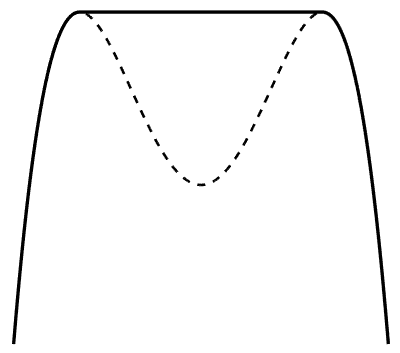
Figure 8. A function $f$, represented by a dotted line, and its concave envelope $f^{\ast}$.

See Figure 8 for an illustration of a function and its concave envelope.

Remark 2.4.

1. As we shall prove in Lemma 6.1, for any $T>0$, $u_{T}\in\operatorname{Lip}(\mathbb{R}^{n})$ and any positive definite matrix $A$, a function $v$ is a viscosity solution of (2.8) if and only if the function

   $$w(x):=v(x)-\dfrac{\langle A^{-1}x,x\rangle}{2T}$$

   is a viscosity solution of (2.9) with

   $$f(x):=u_{T}(x)-\dfrac{\langle A^{-1}x,x\rangle}{2T}.$$

   In other words, $v$ is a viscosity solution of (2.8) if and only if $w$ is the concave envelope of the function $f$ above defined. It gives an alternative way to obtain the viscosity solution of (2.8) in terms of the concave envelope of the function $f$.

2. In the one-dimensional case, the study of problem (1.1) for any strictly convex $H$ can be reduced, after a transformation (see Remark 2.1), to the case $H(p)=p^{2}/2$. Then, equation (2.7) can also be reduced to equation (2.8) in dimension one with $A=1$.

3. Since the concave envelope of a function is unique, we deduce uniqueness of a viscosity solution for problems (2.7) and (2.8). The existence of a viscosity solution can be obtained from Theorem 2.5 by applying the operator $S_{T}^{+}\circ S_{T}^{-}$ to the function $u_{T}$. We note that existence and uniqueness can also be deduced directly by means of the Perron’s method (see [17]).

In analogy with the notion of concave envelope, for any $T>0$ and any positive definite $n\times n$ matrix $A$, we will refer to the viscosity solution of (2.8) as the $\frac{A^{-1}}{T}-$semiconcave envelope of $u_{T}$ in $\mathbb{R}^{n}$. Note that being a viscosity solution of (2.8) implies in particular semiconcavity with linear modulus and constant $\dfrac{\lambda_{n}(A^{-1})}{T}=\dfrac{1}{T\,\lambda_{1}(A)}$. See Subsection 6.2 for a justification of this fact.

Here we state the main result of this subsection, which ensures that the function $u_{T}^{\ast}$ defined in (2.5) is the $\frac{A^{-1}}{T}-$semiconcave envelope of $u_{T}$ in $\mathbb{R}^{n}$.

Theorem 2.5.

Let $u_{T}\in\operatorname{Lip}(\mathbb{R}^{n})$ and $T>0$. Then,

1. If $H$ satisfies (1.2) and the space-dimension is $1$, the function $u_{T}^{\ast}:=S_{T}^{+}(S_{T}^{-}u_{T})$ is the unique viscosity solution of (2.7).

2. If $H$ is given by (2.3), the function $u_{T}^{\ast}:=S_{T}^{+}(S_{T}^{-}u_{T})$ is the unique viscosity solution of (2.8).

See an illustration of this result in Examples 3 and 4. As a consequence of this theorem and Lemma 6.1, we deduce the following corollary which, for the case of a quadratic Hamiltonian, gives an alternative way to obtain $u_{T}^{\ast}$ in terms of the concave envelope of a certain function. This allows one to compute the projection of $u_{T}$ on the set of reachable targets without applying the operators $S_{T}^{-}$ and $S_{T}^{+}$.

Corollary 2.2.

Let $H$ be given by (2.3), $u_{T}\in\operatorname{Lip}(\mathbb{R}^{n})$ and $T>0$. Let $f^{\ast}$ be the concave envelope of

$$f(x):=u_{T}(x)-\dfrac{\langle A^{-1}x,x\rangle}{2T}.$$

Then, the function $u_{T}^{\ast}$ defined in (2.5) satisfies

$$u_{T}^{\ast}(x)=f^{\ast}(x)+\dfrac{\langle A^{-1}x,x\rangle}{2T},\qquad\text{for all}\ x\in\mathbb{R}^{n}.$$

For the particular case

$$H(p)=c\frac{|p|^{2}}{2},\qquad\text{with}\ c>0,$$

the function $u_{T}^{\ast}:=S_{T}^{+}(S_{T}^{-}u_{T})$ is the viscosity solution of

$$\min\left\{v-u_{T},\ -\lambda_{n}\left[D^{2}v\right]+\dfrac{1}{c\,T}\right\}=0.$$

This can be deduced from Theorem 2.5 and Property 6.1, together with the fact that $\lambda_{1}(c^{-1}I_{n})=\lambda_{n}(c^{-1}I_{n})=c^{-1}$. In this case, $u_{T}^{\ast}$ can be identified with the $\frac{1}{c\,T}-$semiconcave envelope of $u_{T}$ in $\mathbb{R}^{n}$, that is, the smallest semiconcave function with linear modulus and constant $\frac{1}{c\,T}$ which is bounded from below by $u_{T}$.

3. Examples

Example 1.

Here we give a particular example of application of Theorem 2.3. We consider the one-dimensional case and the Hamiltonian $H(p)=|p|^{2}/2$. As time horizon and reachable target we choose $T=0.5$ and

(3.1) $$u_{T}(x):=S^{+}_{T}u_{1}(x),\quad\text{where}\quad u_{1}(x):=\left\{\begin{array}[]{ll}1-|x+1|&\text{if}\ -2<x\leq 0\\ 1-|x-1|&\text{if}\ 0<x<2\\ 0&\text{else.}\end{array}\right.$$

Note that $I_{T}(u_{T})\neq\emptyset$, indeed, $u_{1}\in I_{T}(u_{T})$. In Figure 1(a), we can see the function $u_{T}$. We observe that $u_{T}$ is differentiable at all points except for $-1$ and $1$. Computing the lateral derivatives at these two points, the set $X_{T}(u_{T})$ can be easily determined:

$$X_{T}(u_{T})=\mathbb{R}\setminus\left([-1.5,-0.5]\cup[0.5,1.5]\right).$$

The function $\tilde{u}_{0}:=S_{T}^{-}u_{T}$ is represented Figure 1(b). The restriction of $\tilde{u}_{0}$ to the set $X_{T}(u_{T})$ is marked by a red line. In view of Theorem 2.3, the functions in $I_{T}(u_{T})$ are those which coincide with this function on the red line, while they are bigger or equal than it on the black line. In the same plot, we can also see the function $u_{1}$, represented by a dotted line, as another element in $I_{T}(u_{T})$ different to $\tilde{u}_{0}$.

(a) The target $u_{T}$ defined in (3.1)

(b) The initial data $\tilde{u}_{0},u_{1}\in I_{T}(u_{T})$.

Figure 1. The initial data $\tilde{u}_{0}$ and $u_{1}$ satisfy $S_{T}^{+}\tilde{u}_{0}=S_{T}^{+}u_{1}=u_{T}$.

Example 2.

In this example, we give an illustration of the result of Theorem 2.3 for the two-dimensional case. We consider the Hamiltonian $H(p)=|p|^{2}/2,$ as time horizon we have chosen $T=0.5$, and as target, the function

(3.2) $$u_{T}:=S_{T}^{+}u_{2},\quad\text{where}\quad u_{2}(x,y):=\left\{\begin{array}[]{ll}|(x,y)-(-2,0)|-1,&\text{if}\ |(x,y)-(-2,0)|<1\\ 1-|(x,y)-(2,0)|,&\text{if}\ |(x,y)-(2,0)|<1\\ 0,&\text{else.}\end{array}\right.$$

Note that $u_{T}$ is reachable, indeed, $u_{2}\in I_{T}(u_{T})$. We have computed numerically the target $u_{T}=S_{T}^{+}u_{2}$, the function $\tilde{u}_{0}=S_{T}^{-}u_{T}$ and the set of points $X_{T}(u_{T})$ defined in Theorem 2.3. In Figure 2(b), we can see that the function $u_{T}$ has a bump and a well. This function is differentiable at all points except for the top of the bump and the circumference around the well. This is due to the semiconcavity of $u_{T}$ (see Corollary 2.1 and Remark 2.2). We have computed, numerically, the projection on $\mathbb{R}^{2}$ of all the points where $u_{T}$ is differentiable, by the map

$$z\longmapsto z-T\,H_{p}(\nabla u_{T}(z)).$$

We have then obtained the set $X_{T}(u_{T})$, represented by the coloured region in Figure 2(d). Finally, we have computed the function $\tilde{u}_{0}=S_{T}^{-}u_{T}$ by using formula (4.4). It is represented in Figure 2(c).

Now, we can apply Theorem 2.3 in order to construct the set of all the initial conditions in $I_{T}(u_{T})$. The functions in $I_{T}(u_{T})$ are those which coincide with $\tilde{u}_{0}$ on the set $X_{T}(u_{T})$ (coloured region in Figure 2(d)), while on its complement (white region) they are bigger or equal than $\tilde{u}_{0}$.

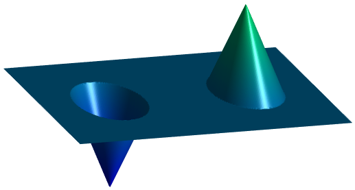
(a) The function $u_{2}$ defined
in (3.2).

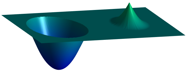
(b) The target $u_{T}$ defined
as $u_{T}:=S_{T}^{+}u_{2}$.

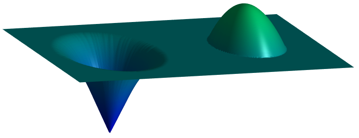
(c) The initial datum $\tilde{u}_{0}$.

(d) The set $X_{T}(u_{T})$ in dark green.

Figure 2. The initial conditions in $I_{T}(u_{T})$ are those functions which coincide with $\tilde{u}_{0}$ on the blue region while on its complement they are bigger or equal than it.

Example 3.

Here, we illustrate the result of Theorem 2.5 for the one-dimensional case and the Hamiltonian $H(p)=|p|^{2}$. We have computed the $\frac{1}{T}-$semiconcave envelopes of the functions $u_{3}$ and $u_{4}$, defined by

(3.3) $$u_{3}(x):=\left\{\begin{array}[]{ll}|x+1|-1&\text{if}\ -2<x\leq 0\\ |x-1|-1&\text{if}\ 0<x<2\\ 0&\text{else.}\end{array}\right.$$

(3.4) $$u_{4}(x):=\left\{\begin{array}[]{ll}1-2|x+1|&\text{if}\ -1.5<x\leq 0\\ 1-2|x-1|&\text{if}\ 0<x<1.5\\ 0&\text{else.}\end{array}\right.$$

with $T=1$ and $T=0.5$ respectively.

In Figure 3(a), we can see the function $u_{3}^{\ast}:=S_{T}^{+}(S_{T}^{-}u_{3})$, with $T=1$. In Figure 3(b), we can see the function $u_{4}^{\ast}:=S_{T}^{+}(S_{T}^{-}u_{4})$, with $T=0.5$. In both plots, the functions $u_{3}$ and $u_{4}$ are represented by a dotted line.

We recall that $u_{3}^{\ast}$ and $u_{4}^{\ast}$ are the projection of $u_{3}$ and $u_{4}$ on the set of reachable targets, and in view of Theorem 2.5, they are the viscosity solution of the obstacle problem (2.8) with $u_{T}=u_{3}$ (resp. $u_{4}$). The function $u_{3}^{\ast}$ (resp. $u_{4}^{\ast}$) has been obtained by solving numerically the problem (2.2) with $u_{T}=u_{3}$ (resp. $u_{T}=u_{4}$), using formula (4.4), and then the problem (1.1) with $u_{0}=S_{T}^{-}u_{3}$ (resp. $u_{0}=S_{T}^{-}u_{4}$), using formula (4.2).

(a) The $1-$semiconcave envelope of the function
$u_{3}$ defined in (3.3).

(b) the $2-$semiconcave envelope of the function
$u_{4}$ defined in (3.4).

Figure 3. The function $u_{3}^{\ast}$ (resp. $u_{4}^{\ast}$) is the smallest reachable target, for $T=1$ (resp. $T=0.5$), bounded from below by $u_{3}$ (resp. $u_{4}$).

Example 4.

We consider now the two-dimensional case with the Hamiltonian

$$H(p):=\dfrac{\langle A\,p,p\rangle}{2},\qquad\text{with}\ A=\left(\begin{array}[]{cc}2&1\\ 1&1\end{array}\right).$$

We have computed numerically the image by $S_{T}^{+}\circ S_{T}^{-}$, with $T=1$, of the function

$$u_{5}(x,y):=\left\{\begin{array}[]{ll}1-|(x,y)-(-1,0)|,&\text{if}\ |(x,y)-(-1,0)|<1\\ 0.5(1-|(x,y)-(1,0)|),&\text{if}\ |(x,y)-(1,0)|<1\\ 0,&\text{else.}\end{array}\right.$$

and with $T=0.5$ for the function

$$u_{6}(x,y)=-u_{5}(x,y).$$

In Figure 4, we can see the function $u_{5}$ at the left and its $A^{-1}-$semiconcave envelope $u_{5}^{\ast}:=S_{1}^{+}(S_{1}^{-}u_{5})$ at the right. In Figure 5, we can see the function $u_{6}$ at the left and its $2A^{-1}-$semiconcave envelope $u_{6}^{\ast}:=S_{0.5}^{+}(S_{0.5}^{-}u_{6})$ at the right.

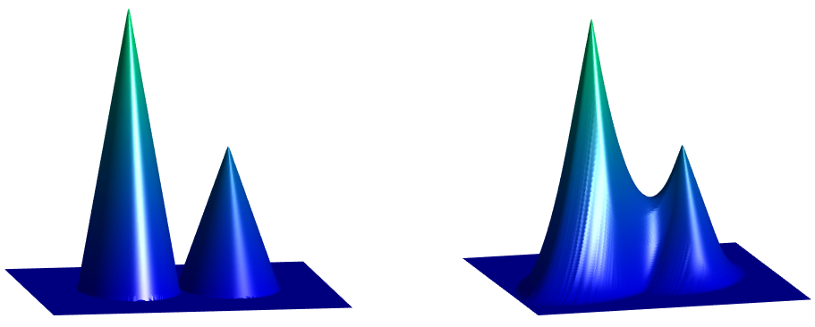
Figure 4. At the left, we see the function $u_{5}$ from Example 4. At the right, we see the function $u_{5}^{\ast}=S_{T}^{+}(S_{T}^{-}u_{5})$ with $T=1$.

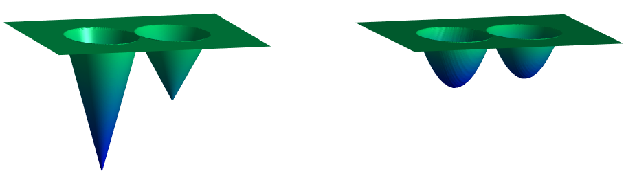
Figure 5. At the left, we see the function $u_{6}$ from Example 4. At the right, we see the function $u_{6}^{\ast}=S_{T}^{+}(S_{T}^{-}u_{6})$ with $T=0.5$.

4. Forward and backward viscosity solutions

We start this section by recalling the definition of viscosity solution for the equation

(4.1) $$\partial_{t}u+H(D_{x}u)=0,\qquad\text{in}\quad[0,T]\times\mathbb{R}^{n},$$

where $H$ is a continuous function $\mathbb{R}^{n}\to\mathbb{R}$.

This notion of solution was introduced by Carndall and Lions in [18] and solved the problem of the lack of uniqueness for generalized solutions to the initial-value problem (1.1), that satisfy the equation (4.1) almost everywhere along with the initial condition $u(0,\cdot)=u_{0}$.

Definition 4.1.

A uniformly continuous function $u:[0,T]\times\mathbb{R}^{n}\to\mathbb{R}$ is called a viscosity solution of (4.1) if the following two statements hold:

1. $u$ is a viscosity subsolution of (1.1): for each $\varphi\in C^{\infty}([0,T]\times\mathbb{R}^{n})$,

   $$\partial_{t}\varphi(t_{0},x_{0})+H(\nabla_{x}\varphi(t_{0},x_{0}))\leq 0$$

   whenever $(t_{0},x_{0})$ is a local maximum of $u-\varphi$.

2. $u$ is a viscosity supersolution of (1.1): for each $\varphi\in C^{\infty}([0,T]\times\mathbb{R}^{n})$,

   $$\partial_{t}\varphi(t_{0},x_{0})+H(\nabla_{x}\varphi(t_{0},x_{0}))\geq 0$$

   whenever $(t_{0},x_{0})$ is a local minimum of $u-\varphi$.

Throughout the paper we will sometimes refer to viscosity solutions as forward viscosity solutions, in contrast with the notion of backward viscosity solution, stated in Definition 4.2. In [18] (see also [7, 13, 25]), it is proved the existence and uniqueness of a viscosity solution for the problem (1.1) for any initial condition $u_{0}\in\operatorname{Lip}(\mathbb{R}^{n})$. This solution can be obtained by means of the Hopf-Lax formula (see [1, 5, 6, 25]). Therefore, the operator $S_{T}^{+}$ defined in the introduction can be written as

(4.2) $$S_{T}^{+}u_{0}(x)=\min_{y\in\mathbb{R}^{n}}\left[u_{0}(y)+T\,L\left(\dfrac{x-y}{T}\right)\right],$$

where, the function $L:\mathbb{R}^{n}\to\mathbb{R}$ is the Legendre transform of $H$, defined as

(4.3) $$L(q):=H^{\ast}(q)=\max_{p\in\mathbb{R}^{n}}[q\cdot p-H(p)].$$

This function corresponds to the Lagrangian in the optimal control problem associated to (1.1). We recall that, under the assumptions (1.2) on $H$, the function $L=H^{\ast}$ is a convex $C^{2}$ function satisfying

$$\lim_{|q|\to\infty}\dfrac{L(q)}{|q|}=+\infty.$$

See for example Section A.2 in [13]. We then deduce that the minimum in the Hopf-Lax formula (4.2) is always attained.

Observe that in the case of a quadratic Hamiltonian of the form (2.3), an elementary computation gives the Lengendre transform of $H$ as

$$L(q)=\dfrac{\langle A^{-1}q,q\rangle}{2}.$$

As announced in the introduction, a key point in our study is the possibility of reversing the direction of time in problem (1.1). This can be done with the notion of backward viscosity solution (see for example [9]).

Definition 4.2.

A function $w:[0,T]\times\mathbb{R}^{n}\longrightarrow\mathbb{R}$ is a backward viscosity solution of (4.1) if the function $v$ obtained from $w$ by “reversing the time”, i.e. $v(t,x):=w(T-t,x)$, is a viscosity solution of

$$\partial_{t}v-H(D_{x}v)=0,\qquad\text{in}\ [0,T]\times\mathbb{R}^{n}.$$

It is clear that a function $w\in C^{1}([0,T]\times\mathbb{R}^{n})$ is a backward viscosity solution if and only if it is a (forward) viscosity solution. However, when one deals with non-smooth solutions, both notions of solution are no longer equivalent. Indeed, viscosity solutions are characterized to be semiconcave, while backward viscosity solutions are semiconvex. See Proposition 4.2 and the Example 5 for an illustration of this phenomenon. The following characterization of backward viscosity solutions follows immediately from the definition.

Proposition 4.1.

A uniformly continuous function $w:[0,T]\times\mathbb{R}^{n}\to\mathbb{R}$ is a backward viscosity solution to (4.1) if and only if the following two properties hold

1. for each $\phi\in C^{\infty}([0,T]\times\mathbb{R}^{n})$,

   $$\partial_{t}\phi(t_{0},x_{0})+H(\nabla_{x}\phi(t_{0},x_{0}))\geq 0$$

   whenever $(t_{0},x_{0})$ is a local maximum of $w-\phi$.

2. for each $\phi\in C^{\infty}([0,T]\times\mathbb{R}^{n})$,

   $$\partial_{t}\phi(t_{0},x_{0})+H(\nabla_{x}\phi(t_{0},x_{0}))\leq 0$$

   whenever $(t_{0},x_{0})$ is a local minimum of $w-\phi$.

Observe that, if we reverse the inequalities in this proposition, we obtain exactly the definition of (forward) viscosity solution (Definition 4.1). We then deduce that any backward solution $w$ satisfies (4.1) at any point where it is differentiable. Using the analogous arguments as for the existence and uniqueness of (forward) viscosity solutions of (1.1), one can prove (see for example [4, 9]) existence and uniqueness of a backward viscosity solution for the terminal-value problem

$$\left\{\begin{array}[]{ll}\partial_{t}w+H(D_{x}w)=0,&\text{in}\ [0,T]\times\mathbb{R}^{n},\\ \vskip 4.2679pt\cr w(T,x)=u_{T}(x),&\text{in}\ \mathbb{R}^{n}.\end{array}\right.$$

Hence, for any $T>0$, the nonlinear operator $S_{T}^{-}$ defined in Section 2 is well defined. Recall that this operator associates, to any $u_{T}\in\operatorname{Lip}(\mathbb{R}^{n})$ the backward viscosity solution of (2.2) at time $0$. In addition, $S_{T}^{-}u_{T}$ can be given by the following representation formula, which is the analogous to the Hopf-Lax formula (4.2) for the operator $S_{T}^{+}$ (see [9]):

(4.4) $$S_{T}^{-}u_{T}(x)=\max_{y\in\mathbb{R}^{n}}\left[u_{T}(y)-T\,L\left(\dfrac{y-x}{T}\right)\right].$$

4.1. Semiconcave and semiconvex functions

Here we recall the following important property of forward and backward viscosity solutions:

Proposition 4.2.

Let $H$ satisfy (1.2), $T>0$, and $u_{0},u_{T}\in\operatorname{Lip}(\mathbb{R}^{n})$. Then, for any bounded set $\mathcal{K}\subset\mathbb{R}^{n}$,

1. the function $S^{+}_{T}u_{0}$ defined in (4.2) is semiconcave in $\mathcal{K}$ with linear modulus;

2. the function $S^{-}_{T}u_{T}$ defined in (4.4) is semiconvex in $\mathcal{K}$ with linear modulus.

See for example Chapter 1 in [13] for a proof of this property. Let us recall the definition of semiconcavity and semiconvexity with linear modulus.

Definition 4.3.

1. We say that a function $f:\mathcal{K}\subset\mathbb{R}^{n}\rightarrow\mathbb{R}$ is semiconcave with linear modulus if it is continuous and there exists $C\geq 0$ such that

   $$f(x+h)+f(x-h)-2f(x)\leq C|h|^{2},\qquad\text{for all $x,h\in\mathbb{R}^{n}$, such that}\ [x-h,x+h]\subset\mathcal{K}.$$

   The constant $C$ above is called a semiconcavity constant for $f$ in $\mathcal{K}$.

2. We say that $f$ is semiconvex if the function $g=-f$ is semiconcave.

Let us illustrate this property with the following example in dimension 1.

Example 5.

We consider the one-dimensional case and the Hamiltonian $H(p)=|p|^{2}/2$. We apply the operators $S^{+}_{T}$ and $S_{T}^{-}$ to the functions $u_{3}$ and $u_{4}$ from Example 3, with $T=1$ and $=0.5$ respectively.

In Figure 6, we can see the function $u_{3}$ represented in both plots by a dotted line. In the plot at the left, we can see the function $S_{T}^{+}u_{3}$. We observe that it is a semiconcave function (roughly speaking, the second derivative is “bounded from above”). However, in the plot at the right, we see that the function $S_{T}^{-}u_{3}$ is a semiconvex function (the second derivative is “bounded from below”). The same behaviour is observed in Figure 7 for the function $u_{4}$ from Example 3.

(a) The function $S_{T}^{+}u_{3}$ with $T=1$.

(b) The function $S_{T}^{-}u_{3}$ with $T=1$.

Figure 6. The dotted line represents the function $u_{3}$ defined in (3.3).

(a) The function $S_{T}^{+}u_{4}$ with $T=0.5$.

(b) The function $S_{T}^{-}u_{4}$ with $T=0.5$

Figure 7. The dotted line represents the function $u_{4}$ defined in (3.4).

The following proposition, whose proof can be found in Chapter 1 in [13], gives an interesting characterization of semiconcave functions with linear modulus. Combining this characterization with Theorem 6.1 in subsection 6.2, it can be easily deduced that any viscosity solution to the differential inequality

$$\lambda_{n}\left[D^{2}v-\dfrac{1}{T}A^{-1}\right]\leq 0,$$

where $A$ is a positive definite matrix, are semiconcave with a linear modulus.

Proposition 4.3.

Given a function $f:\mathbb{R}^{n}\to\mathbb{R}$ and a constant $C\geq 0$, the following properties are equivalent:

1. $f$ is semiconcave with linear modulus and constant $C$;

2. the function $x\mapsto f(x)-\dfrac{C}{2}|x|^{2}$ is concave;

3. there exist two functions $f_{1},f_{2}:\mathbb{R}^{n}\to\mathbb{R}$ such that $f=f_{1}+f_{2}$, $f_{1}$ is concave, $f_{2}\in C^{2}(\mathbb{R}^{n})$ and satisfies $\|D^{2}f_{2}\|_{\infty}\leq C$.

4.2. Proof of Theorem 2.1

This result is a consequence of Proposition 4.4 below, which ensures that for any initial condition, the process of taking alternatively forward and backward viscosity solutions stabilizes after the first step.

Proposition 4.4.

Let $H$ satisfy (1.2), $u_{0}\in\operatorname{Lip}(\mathbb{R}^{n})$ and $T>0$. Set the function

$$\tilde{u}_{0}(x):=S_{T}^{-}(S_{T}^{+}u_{0})(x),\qquad\text{for}\ x\in\mathbb{R}^{n}.$$

Then it holds

(4.5) $$S^{+}_{T}u_{0}=S^{+}_{T}\tilde{u}_{0},\qquad\text{and}\qquad u_{0}(x)\geq\tilde{u}_{0}(x),\quad\text{for all}\ x\in\mathbb{R}^{n}.$$

The following diagram illustrates this property, that was already proved in [9] for a more general setting. We have included here the proof for completeness.

Proof.

By formula (4.2) we have, for any $x\in\mathbb{R}^{n}$,

$$S_{T}^{+}u_{0}(x)\leq u_{0}(y)+T\,L\left(\dfrac{x-y}{T}\right),\quad\text{for all}\ y\in\mathbb{R}^{n}.$$

By the arbitrariness of $x$, we deduce

$$u_{0}(y)\geq S_{T}^{+}u_{0}(x)-T\,L\left(\dfrac{x-y}{T}\right),\quad\text{for all}\ x,y\in\mathbb{R}^{n}.$$

Now, for any fixed $y\in\mathbb{R}^{n}$, taking the maximum over $x$ in the right hand side of the above inequality, and in view of formula (4.4), we obtain $u_{0}(y)\geq S^{-}_{T}(S_{T}^{+}u_{0})(y)$ for any $y\in\mathbb{R}^{n}$. The inequality in (4.5) is then proved.

Now, we use the comparison principle for the viscosity solutions, which can be deduced directly from (4.2) (see also [25] for more details). We obtain

$$S_{T}^{+}u_{0}(x)\geq S_{T}^{+}\tilde{u}_{0}(x),\quad\text{for all}\ x\in\mathbb{R}^{n}.$$

For the reversed inequality, fix $x_{0}\in\mathbb{R}^{n}$ and let $y^{\ast}$ be a minimizer in the right hand side of (4.2). We have

(4.6) $$S^{+}_{T}\tilde{u}_{0}(x_{0})=\tilde{u}_{0}(y^{\ast})+T\,L\left(\dfrac{x_{0}-y^{\ast}}{T}\right).$$

Then, from the definition of $\tilde{u}_{0}$ and formula (4.4), it follows

$$\tilde{u}_{0}(y^{\ast})=\max_{x\in\mathbb{R}^{n}}\left[S_{T}^{+}u_{0}(x)-T\,L\left(\dfrac{x-y^{\ast}}{T}\right)\right]\geq S_{T}^{+}u_{0}(x_{0})-T\,L\left(\dfrac{x_{0}-y^{\ast}}{T}\right).$$

And combining this inequality with (4.6), we obtain

$$S_{T}^{+}u_{0}(x_{0})\leq\tilde{u}_{0}(y^{\ast})+T\,L\left(\dfrac{x_{0}-y^{\ast}}{T}\right)=S_{T}^{+}\tilde{u}_{0}(x_{0}).$$

∎

Using the analogous arguments as in the previous proof, based on the formulas (4.2) and (4.4), we can obtain the following similar result. In this case, we start with a terminal condition $u_{T}\in\operatorname{Lip}(\mathbb{R}^{n})$ and apply first the operator $S_{T}^{-}$, and then the operator $S_{T}^{+}$. This result will be useful in Section 6 for the proof of Theorem 2.5.

Proposition 4.5.

Let $H$ satisfy (1.2), $u_{T}\in\operatorname{Lip}(\mathbb{R}^{n})$ and $T>0$. Set the function

$$u_{T}^{\ast}(x):=S_{T}^{+}(S_{T}^{-}u_{T})(x),\qquad\text{for}\ x\in\mathbb{R}^{n}.$$

Then it holds

(4.7) $$S^{-}_{T}u_{T}=S^{-}_{T}u_{T}^{\ast},\qquad\text{and}\qquad u_{T}(x)\leq u^{\ast}_{T}(x),\quad\text{for all}\ x\in\mathbb{R}^{n}.$$

We conclude this section with the proof of Theorem 2.1.

Proof of Theorem 2.1.

The conclusion follows immediately from Proposition 4.4. Indeed, if $I_{T}(u_{T})\neq\emptyset$, then there exists $u_{0}$ such that $S^{+}_{T}u_{0}=u_{T}$. Now, setting the function $\tilde{u}_{0}=S_{T}^{-}(S_{T}^{+}u_{0})$, after Proposition 4.4 we obtain

$$S_{T}^{+}(S_{T}^{-}u_{T})=S_{T}^{+}(S_{T}^{-}(S_{T}^{+}u_{0}))=S_{T}^{+}\tilde{u}_{0}=S_{T}^{+}u_{0}=u_{T}.$$

Reversely, if $u_{T}$ satisfies $S_{T}^{+}(S_{T}^{-}u_{T})=u_{T}$, we have $S_{T}^{-}u_{T}\in I_{T}(u_{T})$. And the proof is concluded. ∎

5. Initial data construction

Our goal in this section is to prove Theorems 2.3 and 2.4 that, for a time horizon $T>0$ and a reachable target $u_{T}$, give a characterization of the set $I_{T}(u_{T})$ defined in (2.1). For the proofs of these two theorems, we will use the following well-known property of viscosity solutions and Hopf-Lax formula. The proof of this property can be found, for example, in [13].

Proposition 5.1.

Let $H$ satisfy (1.2), $u_{0}\in\operatorname{Lip}(\mathbb{R}^{n})$ and $T>0$. For any fixed $x\in\mathbb{R}^{n}$, the minimizer in the right hand side of (4.2) is unique if and only if the function $S_{T}^{+}u_{0}(\cdot)$ is differentiable at $x$. Moreover, in this case, the minimizer is given by $y^{\ast}=x-T\,H_{p}(\nabla S^{+}_{T}u_{0}(x))$.

Let us now proceed with the proof of Theorem 2.3:

Proof of Theorem 2.3.

First of all note that, after Theorem 2.1, $I_{T}(u_{T})\neq\emptyset$ implies $S_{T}^{+}\tilde{u}_{0}=u_{T}$.

Step 1: (ii) implies (i). Let $u_{0}\in\operatorname{Lip}(\mathbb{R}^{n})$ be any function satisfying the condition (ii) in the enunciate. Since $u_{0}\geq\tilde{u}_{0}$, it follows from the comparison principle (see [25]) that

$$S_{T}^{+}u_{0}(x)\geq S_{T}^{+}\tilde{u}_{0}(x)=u_{T}(x),\qquad\text{for all}\ x\in\mathbb{R}^{n}.$$

Let us prove the reversed inequality. Fix any $x_{0}\in\mathbb{R}^{n}$ such that $u_{T}$ is differentiable at $x_{0}$, and consider $y_{0}=x_{0}-T\,H_{p}(\nabla u_{T}(x_{0}))$. Note that $y_{0}\in X_{T}(u_{T})$ and then, by the assumption (ii), we have $u_{0}(y_{0})=\tilde{u}_{0}(y_{0})$.

Since $u_{T}=S_{T}^{+}\tilde{u}_{0}$ is differentiable at $x_{0}$, we know by Proposition 5.1 that $y_{0}$ is the unique minimizer in the Hopf-Lax formula (4.2) applied to $\tilde{u}_{0}$. Hence,

$$u_{T}(x_{0})=\tilde{u}_{0}(y_{0})+T\,L\left(\dfrac{x_{0}-y_{0}}{T}\right).$$

Applying now the formula (4.2) to the function $u_{0}$, and using $u_{0}(y_{0})=\tilde{u}_{0}(y_{0})$, we obtain

$$S_{T}^{+}u_{0}(x_{0})\leq u_{0}(y_{0})+T\,L\left(\dfrac{x_{0}-y_{0}}{T}\right)=\tilde{u}_{0}(y_{0})+T\,L\left(\dfrac{x_{0}-y_{0}}{T}\right)=u_{T}(x_{0}).$$

We have proved that $S_{T}^{+}u_{0}(x)\leq u_{T}(x)$ for all $x$ where $u_{T}$ is differentiable. Since $u_{T}$ is Lipschitz continuous, by Rademacher’s Theorem, $u_{T}$ is differentiable almost everywhere in $\mathbb{R}^{n}$, and then, by the continuity of viscosity solutions, we conclude that $S_{T}^{+}u_{0}(x)\leq u_{T}(x)$ for all $x\in\mathbb{R}^{n}$.

Step 2: (i) implies (ii). Let $u_{0}\in I_{T}(u_{T})$. Recall that, by Lemma 4.4, we have

(5.1) $$S_{T}^{+}u_{0}=S_{T}^{+}\tilde{u}_{0}=u_{T}\qquad\text{and}\qquad u_{0}(x)\geq\tilde{u}_{0}(x),\ \text{for all}\ x\in\mathbb{R}^{n}.$$

Let us prove that $u_{0}\in I_{T}(u_{T})$ also implies $u_{0}(x)=\tilde{u}_{0}(x)$ for any $x\in X_{T}(u_{T})$. Fix any $x_{0}\in X_{T}(u_{T})$. By the definition of $X_{T}(u_{T})$, there exists $z_{0}\in\mathbb{R}^{n}$ such that $u_{T}$ is differentiable at $z_{0}$ and $x_{0}=z_{0}-T\,H_{p}(\nabla u_{T}(z_{0}))$.

By Proposition 5.1, together with (5.1), it follows that $x_{0}$ is the unique minimizer in Hopf-Lax formula (4.2) with $x=z_{0}$ and initial data $u_{0}$ and $\tilde{u}_{0}$. Hence, we deduce that

$$u_{T}(z_{0})=u_{0}(x_{0})+T\,L\left(\dfrac{z_{0}-x_{0}}{T}\right)=\tilde{u}_{0}(x_{0})+T\,L\left(\dfrac{z_{0}-x_{0}}{T}\right),$$

which implies $u_{0}(x_{0})=\tilde{u}_{0}(x_{0})$. ∎

We now prove a result that characterizes the set $X_{T}(u_{T})$, introduced in Theorem 2.4, as the set of points $x_{0}$ for which there exists a function of the form

$$-T\,L\left(b+\dfrac{x_{0}-x}{T}\right)+c,\qquad\text{with}\ b\in\mathbb{R}^{n},\ c\in\mathbb{R},$$

touching $\tilde{u}_{0}$ from below at $x_{0}$. Note that Theorem 2.4 in Section 2 is a particular case of the following proposition. However, the assumption (2.3) in Theorem 2.4 allows an important simplification of the statement.

Proposition 5.2.

Let $H$ satisfy (1.2) and $T>0$. Let $u_{T}\in\operatorname{Lip}(\mathbb{R}^{n})$ be such that $I_{T}(u_{T})\neq\emptyset$ and take any function $u_{0}\in I_{T}(u_{T})$. Then, for any $x_{0}\in\mathbb{R}^{n}$, the following two statements are equivalent:

1. $x_{0}\in X_{T}(u_{T})$;

2. There exist $p_{0}\in D^{-}u_{0}(x_{0})$ and $c_{0}\in\mathbb{R}$ such that

   $$u_{0}(x_{0})=-T\,L\left(H_{p}(p_{0})\right)+c_{0}\qquad\text{and}$$

   $$u_{0}(x)>-T\,L\left(H_{p}(p_{0})+\dfrac{x_{0}-x}{T}\right)+c_{0},\qquad\forall x\in\mathbb{R}^{n}\setminus\{x_{0}\}.$$

Here we recall the definition of subdifferential of a function $u_{0}\in\operatorname{Lip}(\mathbb{R}^{n})$:

(5.2) $$D^{-}u_{0}(x_{0})=\left\{p\in\mathbb{R}^{n}\,;\ \exists\varphi\in C^{1}(\mathbb{R}^{n}),\ \nabla\varphi(x_{0})=p,\ u_{0}-\varphi\geq 0,\ (u_{0}-\varphi)(x_{0})=0\right\}.$$

Proof.

Let $u_{0}$ be any initial condition in $I_{T}(u_{T})$, i.e. $u_{0}$ satisfies $S_{T}^{+}u_{0}=u_{T}$. Let us recall the definition of $X_{T}(u_{T})$ from Theorem 2.3:

$$X_{T}(u_{T})=\left\{z-T\,H_{p}(\nabla_{x}u_{T}(z))\,;\ \forall z\in\mathbb{R}^{n}\ \text{such that}\ u_{T}\ \text{is differentiable at z}\right\}.$$

Consider any $x_{0}\in X_{T}(u_{T})$. There exists $z_{0}\in\mathbb{R}^{n}$ such that $u_{T}$ is differentiable at $z_{0}$ and

(5.3) $$x_{0}=z_{0}-T\,H_{p}(\nabla_{x}u_{T}(z_{0})).$$

From Proposition 5.1, we deduce that $x_{0}$ is the unique minimizer in the Hopf-Lax formula (4.2) with $x=z_{0}$. Therefore, we have

$$u_{0}(x_{0})=u_{T}(z_{0})-T\,L\left(\dfrac{z_{0}-x_{0}}{T}\right)$$

and

$$u_{0}(x)>u_{T}(z_{0})-T\,L\left(\dfrac{z_{0}-x}{T}\right),\quad\text{for all}\ x\in\mathbb{R}^{n}\setminus\{x_{0}\}.$$

Taking into account these two relations and the identity (5.3), the statement (ii) follows with $c_{0}=u_{T}(z_{0})$ and $p_{0}=\nabla_{x}u_{T}(z_{0})$. We observe that, in view of the definition of subdifferential in (5.2), we have $L_{q}(H_{p}(p_{0}))\in D^{-}u_{0}(x_{0})$, and using the properties of the Legendre transform (see Property 5.1 below), it follows that $p_{0}\in D^{-}u_{0}(x_{0})$.

Conversely, if statement (ii) holds, we see that $x_{0}$ is the unique minimizer in formula (4.2) with $x=z_{0}$, where $z_{0}=x_{0}+T\,H_{p}(p_{0})$. From Proposition 5.1, it follows that $u_{T}$ is differentiable at $z_{0}$ and $\nabla_{x}u_{T}(z_{0})=p_{0}$. Then $x_{0}\in X_{T}(u_{T})$. ∎

Here we recall the following elementary property of the Legendre transform that has been used in the previous proof. See for example Section A.2 in [13] for the proof of this property.

Property 5.1.

Under the assumptions (1.2) on $H$, the function $L$ defined by

$$L(q)=\max_{p\in\mathbb{R}^{n}}[q\cdot p-H(p)]$$

is a strictly convex $C^{2}$ function, and its gradient $L_{q}$ is a $C^{1}$ diffeomorphism from $\mathbb{R}^{n}$ to $\mathbb{R}^{n}$ satisfying

$$H_{p}(p)=(L_{q})^{-1}(p)\quad\text{and}\quad\left[H_{pp}(p)\right]^{-1}=L_{qq}\left(H_{p}(p)\right),\quad\text{for all}\ p\in\mathbb{R}^{n}.$$

We end the section with the proof of Theorem 2.4.

Proof of Theorem 2.4.

The result is a particular case of Proposition 5.2. Note that in this case $H$ is given by (2.3). Hence, we have

(5.4) $$H_{p}(p)=A\,p\qquad\text{and}\qquad L(q)=H^{\ast}(q)=\dfrac{\langle A^{-1}q,q\rangle}{2}.$$

Consider any $u_{0}\in I_{T}(u_{T})$. By Proposition 5.2, if $x_{0}\in X_{T}(u_{T})$, then we have

$$u_{0}(x_{0})=-T\,L(H_{p}(p_{0}))+c_{0},$$

and

$$u_{0}(x)>-T\,L\left(H_{p}(p_{0})+\dfrac{x_{0}-x}{T}\right)+c_{0},\quad\forall x\in\mathbb{R}^{n}\setminus\{x_{0}\},$$

for some $p_{0}\in D^{-}u_{0}(x_{0})$ and $c_{0}\in\mathbb{R}$. The identities in (5.4) and a simple computation give

$$u_{0}(x_{0})=-T\,\dfrac{\langle A\,p_{0},p_{0}\rangle}{2}+c_{0},$$

and

$$u_{0}(x)>-\dfrac{\langle A^{-1}(x_{0}-x),\,x_{0}-x\rangle}{2T}-\langle p_{0},\,x_{0}-x\rangle-T\,\dfrac{\langle A\,p_{0},\,p_{0}\rangle}{2}+c_{0},\quad\forall x\in\mathbb{R}^{n}\setminus\{x_{0}\}.$$

The statement (ii) in Theorem 2.4 then holds with

$$b:=\dfrac{1}{T}A^{-1}x_{0}+p_{0}\qquad\text{and}\qquad c:=-\dfrac{\langle A^{-1}x_{0},x_{0}\rangle}{2T}-\langle p_{0},\,x_{0}\rangle-T\dfrac{\langle A\,p_{0},\,p_{0}\rangle}{2}+c_{0}.$$

Now, let $x_{0}\in\mathbb{R}^{n}$ be such that condition (ii) in Theorem 2.4 holds for some $b\in\mathbb{R}^{n}$ and $c\in\mathbb{R}$. In view of the definition of subdifferential (5.2), we see that

$$p_{0}:=-\dfrac{1}{T}A^{-1}x_{0}+b\in D^{-}u_{0}(x_{0}).$$

With this choice of $p_{0}$ and taking $c_{0}:=u_{0}(x_{0})+T\,\dfrac{\langle A\,p_{0},p_{0}\rangle}{2}$, it is not difficult to verify that condition (ii) in Proposition 5.2 holds, and then $x_{0}\in X_{T}(u_{T})$.

∎

6. Semiconcave envelopes

In this section, we study the following fully nonlinear obstacle problem

(6.1) $$\min\left\{v-u_{T},\,-\lambda_{n}\left[D^{2}v-\frac{\left[H_{pp}(Dv)\right]^{-1}}{T}\right]\right\}=0,$$

where $H$ is a function satisfying (1.2), and $u_{T}\in\operatorname{Lip}(\mathbb{R}^{n})$ and $T>0$ are given.

We first prove Theorem 2.5, which ensures that, for the one-dimensional case and when $H$ is quadratic (i.e. given by (2.3)), the function $u_{T}^{\ast}:=S_{T}^{+}(S_{T}^{-}u_{T})$ is a viscosity solution of (6.1). This function is obtained by solving the terminal-value problem (2.2) and then the initial-value problem (1.1) with initial condition $S^{-}_{T}u_{T}$. Afterwards, we will discuss the connection of equation (6.1) with the notion of semiconcave envelope and we will give the proofs of Theorem 2.2 and Corollary 2.1.

6.1. Proof of Theorem 2.5

We start by recalling the definition of viscosity solution to problem (6.1), in terms of sub- and supersolutions.

Definition 6.1.

Let $u_{T}\in\operatorname{Lip}(\mathbb{R}^{n})$ be a given function.

1. The upper semicontinuous function $v$ is a viscosity subsolution of (6.1) if for every twice-differentiable function $\phi(\cdot)$,

   $$\phi(x_{0})-u_{T}(x_{0})\leq 0\quad\text{or}\quad-\lambda_{n}\left[D^{2}\phi(x_{0})-\dfrac{\left[H_{pp}(\nabla\phi(x_{0}))\right]^{-1}}{T}\right]\leq 0,$$

   whenever $x_{0}$ is a local maximum of $v-\phi$ and $v(x_{0})=\phi(x_{0})$.

2. The lower semicontinuous function $v$ is a viscosity supersolution of (6.1) if for every twice-differentiable function $\phi(\cdot)$,

   $$\phi(x_{0})-u_{T}(x_{0})\geq 0\quad\text{and}\quad-\lambda_{n}\left[D^{2}\phi(x_{0})-\dfrac{\left[H_{pp}(\nabla\phi(x_{0}))\right]^{-1}}{T}\right]\geq 0,$$

   whenever $x_{0}$ is a local minimum of $v-\phi$ and $v(x_{0})=\phi(x_{0})$.

3. The continuous function $v$ is a viscosity solution of (6.1) if it is at the same time a viscosity super- and subsolution.

See [17, 22] for more details on the theory of viscosity solutions, and [28] for the particular case of viscosity solutions to degenerate elliptic obstacle problems similar to (6.1).

Proof of Theroem 2.5.

Since most of the steps in the proof are in common for the one-dimensional case and the quadratic case in any space dimension, we shall treat both cases at the same time, considering a general convex $H$ in any space-dimension. We will treat both cases separately only when it is needed. In both cases, the uniqueness of a viscosity solution can be deduced from Remark 2.4.

Consider $n\geq 1$, $H$ satisfying (1.2) and let $L=H^{\ast}$. Let us start by proving that $u_{T}^{\ast}:=S_{T}^{+}(S_{T}^{-}u_{T})$ is a viscosity supersolution. Fix $x_{0}\in\mathbb{R}^{n}$ and let $\phi$ be a twice-differentiable function such that $u_{T}^{\ast}(x_{0})=\phi(x_{0})$ and $\phi(x)\leq u_{T}^{\ast}(x)$ for any $x\in B_{\delta}(x_{0})$, with $\delta>0$ small.

Since $u_{T}^{\ast}(x_{0})=\phi(x_{0})$, using the inequality in Proposition 4.5 it follows that $\phi(x_{0})\geq u_{T}(x_{0})$. By the definition of $u_{T}^{\ast}$ and formula (4.2), there exists $y^{\ast}\in\mathbb{R}^{n}$ such that

(6.2) $$\phi(x_{0})=u_{T}^{\ast}(x_{0})=S_{T}^{-}u_{T}(y^{\ast})+T\,L\left(\dfrac{x_{0}-y^{\ast}}{T}\right).$$

In the other hand, using the equality in Proposition 4.5, together with formula (4.4), we have

$$S_{T}^{-}u_{T}(y^{\ast})=S_{T}^{-}u_{T}^{\ast}(y^{\ast})\geq u_{T}^{\ast}(x)-T\,L\left(\dfrac{x-y^{\ast}}{T}\right),\quad\text{for all}\ x\in\mathbb{R}^{n},$$

and this implies

$$\phi(x)\leq u_{T}^{\ast}(x)\leq S_{T}^{-}u_{T}(y^{\ast})+T\,L\left(\dfrac{x-y^{\ast}}{T}\right)\quad\text{for all}\ x\in B_{\delta}(x_{0}).$$

This inequality, combined with (6.2), implies that the function

$$\Psi(x):=S_{T}^{-}u_{T}(y^{\ast})+T\,L\left(\dfrac{x-y^{\ast}}{T}\right)$$

satisfies $\phi(x_{0})=\Psi(x_{0})$ and $\phi(x)\leq\Psi(x)$ for all $x\in B_{\delta}(x_{0})$.

Hence, we deduce that $\nabla\phi(x_{0})=\nabla\Psi(x_{0})$ and the Hessian matrix $D^{2}(\phi(x_{0})-\Psi(x_{0}))$ is semidefinite negative.

We then have

$$\nabla\phi(x_{0})=L_{q}\left(\dfrac{x_{0}-y^{\ast}}{T}\right),\quad\text{and}\quad-\lambda_{n}\left[D^{2}\phi(x_{0})-\dfrac{1}{T}L_{qq}\left(\dfrac{x_{0}-y^{\ast}}{T}\right)\right]\geq 0.$$

Now, using Property 5.1, we obtain $\dfrac{x_{0}-y^{\ast}}{T}=H_{p}(\nabla\phi(x_{0}))$, and then

$$-\lambda_{n}\left[D^{2}\phi(x_{0})-\dfrac{L_{qq}\left(H_{p}(\nabla\phi(x_{0}))\right)}{T}\right]\geq 0.$$

Using again Property 5.1, we conclude

$$-\lambda_{n}\left[D^{2}\phi(x_{0})-\dfrac{\left[H_{pp}\left(\nabla\phi(x_{0})\right)\right]^{-1}}{T}\right]\geq 0.$$

Next, we prove that $u_{T}^{\ast}$ is also a viscosity subsolution. Fix $x_{0}\in\mathbb{R}^{n}$ and let $\phi$ be a twice-differentiable function such that $u_{T}^{\ast}(x_{0})=\phi(x_{0})$ and $\phi(x)\geq u_{T}^{\ast}(x)$ for any $x\in B_{\delta}(x_{0})$, with $\delta>0$ small. We shall prove that

if $$-\lambda_{n}\left[D^{2}\phi(x_{0})-\dfrac{\left[H_{pp}\left(\nabla\phi(x_{0})\right)\right]^{-1}}{T}\right]>0 \phi(x_{0})=u_{T}(x_{0})$$, then .

Let us suppose that $\lambda_{n}\left[D^{2}\phi(x_{0})-\dfrac{\left[H_{pp}\left(\nabla\phi(x_{0})\right)\right]^{-1}}{T}\right]<0$. If we take $y_{0}=x_{0}-T\,H_{p}\left(\nabla\phi(x_{0})\right)$, using Property 5.1, we obtain

$$\lambda_{n}\left[D^{2}\phi(x_{0})-\dfrac{1}{T}L_{qq}\left(\dfrac{x_{0}-y_{0}}{T}\right)\right]<0.$$

This implies that the function

$$\psi(x):=\phi(x)-T\,L\left(\dfrac{x-y_{0}}{T}\right),$$

is strictly concave in a neighbourhood of $x_{0}$. In addition, by the choice of $y_{0}$, we can use Property 5.1 to prove that $\nabla\psi(x_{0})=0$.

This implies that $\psi$ has a strict local maximum at $x_{0}$, i.e. there exist $\delta^{\prime}>0$ small and a constant $C\in\mathbb{R}$, such that

$$\psi(x_{0})=C\quad\text{and}\quad\psi(x)<C\ \text{for all}\ x\in B_{\delta^{\prime}}(x_{0})\setminus\{x_{0}\}.$$

Taking $\delta^{\prime\prime}=\min\{\delta,\delta^{\prime}\}$, since $\phi\geq u_{T}^{\ast}$ in $B_{\delta}(x_{0})$ and $\phi(x_{0})=u_{T}^{\ast}(x_{0})$, we deduce that the function

$$\Psi(x):=u_{T}^{\ast}(x)-T\,L\left(\dfrac{x-y_{0}}{T}\right)$$

also satisfies

(6.3) $$\Psi(x_{0})=C\quad\text{and}\quad\Psi(x)<C,\ \text{for all}\ x\in B_{\delta^{\prime\prime}}(x_{0})\setminus\{x_{0}\}.$$

Now, we shall prove that for the one-dimensional case and for the case when $H$ is quadratic in any space-dimension, $x_{0}$ is in fact the unique maximizer of $\Psi$ over $\mathbb{R}^{n}$. Here, we treat both cases separately:

Case 1: One-dimensional case. Let us suppose, for a contradiction, that there exists $x_{1}\in\mathbb{R}\setminus\{x_{0}\}$ such that $\Psi(x_{1})\geq\Psi(x_{0})$. Assume without loss of generality that $x_{0}<x_{1}$, and let

$$x_{2}:=\underset{x\in[x_{0},x_{1}]}{\text{argmin}}\Psi(x).$$

From (6.3), we deduce that $x_{2}$ is an interior point of $[x_{0},x_{1}]$ and satisfies $\Psi(x_{2})<\Psi(x_{0})$.

Then, using the definition of subdifferential in (5.2), it is not difficult to prove that $0\in D^{-}\Psi(x_{2})$, and by the definition of $\Psi$, we have

(6.4) $$L_{q}\left(\dfrac{x_{2}-y_{0}}{T}\right)\in D^{-}u_{T}^{\ast}(x_{2}).$$

Now, observe that, by Proposition 4.2, we have that $u_{T}^{\ast}=S_{T}^{+}(S_{T}^{-}u_{T})$ is a semiconcave function. From a well-known property of semiconcave functions (Proposition 3.3.4 in [13]), the superdifferential of a semiconcave function is nonempty for any $x$.

Hence, we have

$$D^{-}u_{T}^{\ast}(x_{2})\neq\emptyset\quad\text{and}\quad D^{+}u_{T}^{\ast}(x_{2})\neq\emptyset,$$

and by Proposition 3.1.5 in [13], we deduce that $u_{T}^{\ast}$ is differentiable at $x_{2}$. Indeed, in view of (6.4), we have

$$\nabla u_{T}^{\ast}(x_{2})=L_{q}\left(\dfrac{x_{2}-y_{0}}{T}\right).$$

Now, by Proposition 5.1, the unique minimizer in the Hopf-Lax formula (4.2), with $u_{0}=S_{T}^{-}u_{T}$ and $x=x_{2}$, is given by

$$y^{\ast}=x_{2}-T\,H_{p}(\nabla u_{T}^{\ast}(x_{2}))=x_{2}-T\,H_{p}\left(L_{q}\left(\dfrac{x_{2}-y_{0}}{T}\right)\right)=y_{0}.$$

Here we used Property 5.1. Therefore, we have

$$u_{T}^{\ast}(x_{2})=S_{T}^{-}u_{T}(y_{0})+T\,L\left(\dfrac{x_{2}-y_{0}}{T}\right).$$

This implies that $\Psi(x_{2})=S_{T}^{-}u_{T}(y_{0})$, and using Proposition 4.5, we deduce

$$\Psi(x_{2}) = S_{T}^{-}u_{T}(y_{0})=S_{T}^{-}u_{T}^{\ast}(y_{0})$$

$$= \max_{x\in\mathbb{R}}\left\{u_{T}^{\ast}(x)-T\,L\left(\dfrac{x-y_{0}}{T}\right)\right\}$$

$$\geq u_{T}^{\ast}(x_{0})-T\,L\left(\dfrac{x_{0}-y_{0}}{T}\right)=\Psi(x_{0}),$$

and this contradicts $\Psi(x_{2})<\Psi(x_{0})$. We then deduce that $x_{0}$ is the unique maximizer of $\Psi$.

Case 2: $H$ quadratic. Suppose that $H$ is given by (2.3) for some positive definite matrix $A$. As we have proved in the first part of this proof, $u_{T}^{\ast}$ is a viscosity supersolution of (6.1). Since in this case $H_{pp}(p)=A$ for all $p\in\mathbb{R}^{n}$. We have that $u_{T}^{\ast}$ satisfies the inequality $-\lambda_{n}\left[D^{2}u_{T}^{\ast}-\dfrac{A^{-1}}{T}\right]\geq 0$ in a viscosity sense.

Then, since $L_{qq}(q)=A^{-1}$ for all $q\in\mathbb{R}^{n}$, we deduce that $\Psi$ satisfies $-\lambda_{n}[D^{2}\Psi]\geq 0$ in a viscosity sense, and this implies that $\Psi$ is a concave function (see Theorem 6.1 below). From the concavity of $\Psi$, together with (6.3), we obtain that $x_{0}$ is the unique maximizer of $\Psi$.

In both cases, we have proved that

(6.5) $$\Psi(x_{0})=C\quad\text{and}\quad\Psi(x)<C,\ \text{for all}\ x\in\mathbb{R}^{n}\setminus\{x_{0}\}.$$

Therefore, we have

(6.6) $$C=u_{T}^{\ast}(x_{0})-T\,L\left(\dfrac{x_{0}-y_{0}}{T}\right)$$

and

(6.7) $$C>u_{T}^{\ast}(x)-T\,L\left(\dfrac{x-y_{0}}{T}\right),\ \text{for all}\ x\in\mathbb{R}^{n}\setminus\{x_{0}\},$$

and after the equality in Proposition 4.5 and formula (4.4), we obtain

(6.8) $$S^{-}_{T}u_{T}(y_{0})=S_{T}^{-}u_{T}^{\ast}(y_{0})=C.$$

Finally, applying (6.7) and the inequality in Proposition 4.5, we obtain

$$S^{-}_{T}u_{T}(y_{0})=C>u_{T}(x)-T\,L\left(\dfrac{x-y_{0}}{T}\right),\qquad\text{for all}\ x\in\mathbb{R}^{n}\setminus\{x_{0}\},$$

which, combined with (6.8), implies $u_{T}(x_{0})-T\,L\left(\dfrac{x_{0}-y_{0}}{T}\right)=C$, since the maximum in formula (4.4) is always attained. The equality $\phi(x_{0})=u_{T}^{\ast}(x_{0})=u_{T}(x_{0})$ then follows from (6.6) and the choice of $\phi$. ∎

Remark 6.1.

Observe that in Case 1 of this proof, we used that in the one-dimensional case, between two local maxima of a continuous function there is always a local minimum. In higher dimension, this property is no longer true since there can be saddle points. Therefore, the same argument cannot be used to treat the multidimensional case. However, by assuming that the Hessian matrix of $H$ is constant over $\mathbb{R}^{n}$, we can prove that $\Psi$ is concave and then deduce that $x_{0}$ is the unique maximizer of $\Psi$.

6.2. Semiconcave envelopes and proof of Theorem 2.2

It is well known that twice-differentiable convex functions are characterized by the property that the Hessian is everywhere positive semidefinite, and analogously, twice-differentiable concave functions are those such that the Hessian is everywhere negative semidefinite. This result can be generalized to continuous functions by the following result proved by Oberman in [28].

Theorem 6.1 (Oberman [28]).

1. The continuous function $v:\mathbb{R}^{n}\to\mathbb{R}$ is convex if and only if it is a viscosity solution of $\lambda_{1}[D^{2}v]\geq 0$.

2. The continuous function $v:\mathbb{R}^{n}\to\mathbb{R}$ is concave if and only if it is a viscosity solution of $\lambda_{n}[D^{2}v]\leq 0$.

The definition of viscosity solution for these two inequalities is the same as Definition 6.2 below, adapted in an obvious way. In [28], it was proved that the convex envelope of a given function $f:\mathbb{R}^{n}\to\mathbb{R}$ is the viscosity solution of the obstacle problem

(6.9) $$\max\{v-f,\,-\lambda_{1}[D^{2}v]\}=0.$$

In [28], the solution of (6.9) is also identified with the value function of a stochastic optimal control problem.

Analogously to the equation for the convex envelope, the concave envelope of $f$ is the unique viscosity solution of

$$\min\{v-f,\,-\lambda_{n}[D^{2}v]\}=0.$$

For related literature concerning equations involving operators like $\lambda_{1}[\cdot]$ and $\lambda_{n}[\cdot]$ and its relation with convex/concave envelopes and with stochastic control theory we refer to [10, 11, 12, 20, 29, 30] and the references therein.

In our case, the viscosity solution $v$ of the obstacle problem (6.1) is not necessarily concave. However, if $H$ is given by (2.3), the solution of (6.1) satisfies the inequality

$$\lambda_{n}\left[D^{2}v-\dfrac{1}{T}A^{-1}\right]\leq 0,$$

in the viscosity sense of Definition 6.2. This implies, using Theorem 6.1, that the function

$$x\longmapsto v(x)-\dfrac{\langle A^{-1}x,x\rangle}{2T}$$

is concave. Hence, applying the characterization of semiconcave functions in Proposition 4.3, we deduce that $v$ is semiconcave with linear modulus and constant

$$C=\lambda_{n}\left[\dfrac{A^{-1}}{T}\right]=\dfrac{1}{T\lambda_{1}[A]}.$$

Next we prove that, when $H$ is quadratic, the solution to the problem (6.1) can be given in terms of the concave envelope of a certain auxiliary function $f$. This result proves the conclusion of Corollary 2.2.

Lemma 6.1.

Let $H$ be given by (2.3) for some definite positive $n\times n$ matrix $A$. Let $T>0$ and $u_{T}\in\operatorname{Lip}(\mathbb{R}^{n})$. The function $v$ is the viscosity solution of (6.1) if and only if the function

$$w(x):=v(x)-\dfrac{\langle A^{-1}x,x\rangle}{2T}$$

is the viscosity solution of

(6.10) $$\min\left\{w-f,\,-\lambda_{n}[D^{2}w]\right\}=0,$$

where

$$f(x):=u_{T}(x)-\dfrac{\langle A^{-1}x,x\rangle}{2T}.$$

Proof.

We recall that the definition of viscosity solution of (6.10) is the same as Definition 6.1 replacing $H$ by $0$ and $u_{T}$ by $f$.

We need to prove that $v$ is a viscosity supersolution (resp. subsolution) of (6.1) if and only if $w$ is a viscosity supersolution (resp.subsolution) of (6.10). We only give the proof for the equivalence of viscosity supersolution since the same argument works for the viscosity subsolutions.

Let $v$ be a viscosity supersolution of (6.1). For any $x_{0}\in\mathbb{R}^{n}$, take $\phi$ any twice-differentiable function such that $w(x_{0})=\phi(x_{0})$ and $x_{0}$ is a local minimum for $w-\phi$. Using the definition of $w$ in the enunciate of the lemma, this implies that

$$v(x_{0})-\left(\dfrac{\langle A^{-1}x_{0},x_{0}\rangle}{2T}+\phi(x_{0})\right)=0$$

and

$$0\leq v(x)-\underbrace{\left(\dfrac{\langle A^{-1}x,x\rangle}{2T}+\phi(x)\right)}_{\varphi(x)},\quad\text{for all}\ x\in B_{\delta}(x_{0}),$$

for some $\delta>0$ small. Observe that $\varphi$ is a twice differentiable function such that $v(x_{0})=\varphi(x_{0})$ and $x_{0}$ is a local minimum for $v-\varphi$. Then, since $v$ is a viscosity supersolution of (6.1), we have

$$\varphi(x_{0})\geq u_{T}(x_{0})\quad\text{and}\quad-\lambda_{n}\left[D^{2}\varphi(x_{0})-\dfrac{A^{-1}}{T}\right]\geq 0.$$

Using the definition of $f$ and the choice of $\varphi$, this implies that

$$\phi(x_{0})\geq u_{T}(x_{0})-\dfrac{\langle A^{-1}x_{0},x_{0}\rangle}{2T}=f(x_{0})\quad\text{and}\quad-\lambda_{n}\left[D^{2}\phi(x_{0})\right]\geq 0.$$

We have then proved that $w$ is a viscosity supersolution of (6.10). Similarly, we can prove that if $w$ is a viscosity supersolution of (6.10), then $v$ is a viscosity supersolution of (6.1). ∎

We now turn our attention to the reachability condition given in Theorem 2.2: if $H$ is quadratic or if the space dimension is 1, then the target $u_{T}$ is reachable if and only if $u_{T}$ satisfies the inequality

(6.11) $$\lambda_{n}\left[D^{2}u_{T}-\dfrac{\left[H_{pp}(Du_{T})\right]^{-1}}{T}\right]\leq 0$$

in the viscosity sense. Let us make precise the definition of viscosity solution of the above inequality.

Definition 6.2.

The upper semicontinuous function $u_{T}$ is a viscosity solution of (6.11) if for every twice-differentiable function $\phi(\cdot)$,

$$\lambda_{n}\left[D^{2}\phi(x)-\dfrac{\left[H_{pp}(\nabla\phi(x))\right]^{-1}}{T}\right]\leq 0,\quad\text{whenever $x$ is a local minimum of $u_{T}-\phi$}.$$

Observe that it is equivalent to say that $u_{T}$ is a viscosity supersolution of (6.1) (see (ii) in Definition 6.1).

Proof of Theorem 2.2.

The result can be deduced from Theorems 2.1 and 2.5. Let $T>0$ be fixed. From Theorem 2.1, a function $u_{T}$ satisfies $I_{T}(u_{T})\neq\emptyset$ if and only if

$$u_{T}^{\ast}=S_{T}^{+}(S_{T}^{-}u_{T})=u_{T}.$$

In view of Theorem 2.5, if $n=1$ or if $H$ is given by (2.3), this is equivalent to say that $u_{T}$ is the viscosity solution of the obstacle problem (6.1)

Observe that, in view of Definition 6.1, $u_{T}$ is always a viscosity subsolution of (6.1). In order to be also a viscosity supersolution, it only needs to verify the inequality

$$\lambda_{n}\left[D^{2}u_{T}(x)-\dfrac{\left[H_{pp}(Du_{T})\right]^{-1}}{T}\right]\leq 0$$

in the viscosity sense of Definition 6.2. We then deduce that $u_{T}$ is a viscosity solution of the obstacle problem (6.1) if and only if $u_{T}$ verifies this inequality in the viscosity sense. ∎

We end this section with the proof of Corollary 2.1, that links the reachability of a target $u_{T}$ with its semiconcavity constant. At some point in the proof, it will be necessary to use the following elementary property from linear algebra:

Property 6.1.

For any two $n\times n$ symmetric matrices $X$ and $Y$, the following inequality holds:

$$\lambda_{1}(X)+\lambda_{n}(Y)\leq\lambda_{n}(X+Y)\leq\lambda_{n}(X)+\lambda_{n}(Y).$$

This property can be deduced from the formula

$$\lambda_{1}(X)=\inf_{p\in\mathbb{R}^{n}}\dfrac{\langle X\,p,p\rangle}{|p|^{2}}\quad\text{and}\quad\lambda_{n}(X)=\sup_{p\in\mathbb{R}^{n}}\dfrac{\langle X\,p,p\rangle}{|p|^{2}}.$$

Proof of Corollary 2.1.

Let $u_{T}$ be a Lipschitz function such that $I_{T}(u_{T})\neq\emptyset$. From Theorem 2.2 we have that $u_{T}$ is a viscosity solution of

$$\lambda_{n}\left[D^{2}u_{T}-\dfrac{1}{T}A^{-1}\right]\leq 0.$$

Hence, in view of Theorem 6.1, the function $x\mapsto u_{T}(x)-\dfrac{\langle A^{-1}x,x\rangle}{2T}$ is concave. Using the characterization of semiconcave functions in Proposition 4.3, we deduce that $u_{T}$ is semiconcave with linear modulus and constant $\frac{1}{T\lambda_{1}[A]}$.

Let us prove now the second statement. Suppose that $u_{T}$ is semiconcave with linear modulus and constant

$$C=\dfrac{1}{T\lambda_{n}[A]}=\lambda_{1}\left[\dfrac{A^{-1}}{T}\right].$$

Using the equivalence (i)-(ii) in Proposition 4.3, we have that the function

$$f(x):=u_{T}(x)-\dfrac{\lambda_{1}[A^{-1}]}{2T}|x|^{2}$$

is concave. Hence, applying Theorem 6.1, we have that $f$ is a viscosity solution of $\lambda_{n}[D^{2}f]\leq 0$.

We then have that $u_{T}$ satisfies

(6.12) $$\lambda_{n}\left[D^{2}u_{T}-\dfrac{\lambda_{1}[A^{-1}]}{T}I_{n}\right]\leq 0$$

in the viscosity sense, where $I_{n}$ is the $n\times n$ identity matrix. Now, we combine (6.12) with Property 6.1, along with the fact that $\lambda_{1}[cI_{n}]=c$, to obtain

$$0 \geq \lambda_{n}\left[D^{2}u_{T}-\dfrac{\lambda_{1}[A^{-1}]}{T}I_{n}\right]$$

$$\geq \lambda_{n}[D^{2}u_{T}]+\lambda_{1}\left[-\dfrac{\lambda_{1}[A^{-1}]}{T}I_{n}\right]$$

$$= \lambda_{n}[D^{2}u_{T}]-\dfrac{\lambda_{1}[A^{-1}]}{T}.$$

Finally, combining this inequality again with Property 6.1, we obtain

$$\lambda_{n}\left[D^{2}u_{T}-\dfrac{1}{T}A^{-1}\right] \leq \lambda_{n}[D^{2}u_{T}]+\dfrac{\lambda_{n}[-A^{-1}]}{T}$$

$$= \lambda_{n}[D^{2}u_{T}]-\dfrac{\lambda_{1}[A^{-1}]}{T}\leq 0.$$

And from Theorem 2.2, we conclude that $I_{T}(u_{T})\neq\emptyset$. ∎

7. Conclusions and perspectives

The first goal in this work was to characterize the set of reachable targets $u_{T}$ for a time-evolution Hamilton-Jacobi equation of the form (1.1). Using the inversion of the direction of time in the equation and the notion of backward viscosity solution we proved, in Theorem 2.1, that the reachable targets are the fix-points of the composition operator $S_{T}^{+}\circ S_{T}^{-}$ (see the precise definition of $S_{T}^{+}$ and $S_{T}^{-}$ in Section 4). We note that this result can be extended, using similar arguments, to Hamilton-Jacobi equations with a Hamiltonian depending on $x$, i.e.

$$\partial_{t}u+H(x,D_{x}u)=0.$$

In addition, for the one-dimensional case and for quadratic Hamiltonians in any space-dimension we characterize, in Theorem 2.2, the set of reachable targets as the viscosity solutions to the differential inequality

(7.1) $$\lambda_{n}\left[D^{2}u_{T}-\dfrac{\left(H_{pp}(Du_{T})\right)^{-1}}{T}\right]\leq 0.$$

Since $H$ is assumed to be strictly convex (see hypothesis (1.2)), inequality (7.1) implies in particular that the reachable targets are semiconcave functions with linear modulus and constant

$$C=\dfrac{1}{T\,K_{u_{T}}},\qquad\text{where}\quad K_{u_{T}}=\min_{|p|\leq\operatorname{Lip}(u_{T})}H_{pp}(p)>0.$$

Here, $\operatorname{Lip}(u_{T})$ is the Lipschitz constant of $u_{T}$.

Although the semiconcavity of the viscosity solutions is a well-known property of Hamilton-Jacobi equations, we point out that inequality (7.1) gives a necessary and sufficient condition for the reachability of the target. Inequality (7.1) describes exactly the semiconcavity that is needed for a target to be reachable. In one space dimension, inequality (7.1) can be written as

$$\partial_{xx}u_{T}-\left(T\,H_{pp}(\partial_{x}u_{T})\right)^{-1}\leq 0,$$

and is the analogous to the one-sided Lipschitz condition for scalar conservation laws (see for example [16, 24]). We recall that the transformation

$$u(t,x)\longmapsto v(t,x):=\partial_{x}u(t,x),$$

transforms any viscosity solution of the Hamilton-Jacobi equation (1.1) in one-space dimension, into an entropy solution of the scalar conservation law

$$\partial_{t}v+\partial_{x}(H(v))=0.$$

In higher dimension, the hypothesis of $H_{pp}(p)$ being constant seems to be crucial in our proof, and we do not know if the inequality (7.1) also provides a necessary and sufficient reachability condition for general strictly convex Hamiltonians in dimension higher than 1. For the case of a Hamiltonian $H(x,p)$ depending on $x$, the existence of an inequality similar to (7.1) characterizing the set of reachable targets is a probably difficult problem.

Our second goal in this work was to construct, for any reachable target $u_{T}$, the set of all the initial conditions $u_{0}$ satisfying $S_{T}^{+}u_{0}=u_{T}$. In Theorem 2.3, we proved that this construction can be carried out by obtaining two elements:

1. the function $\tilde{u}_{0}:=S_{T}^{-}u_{T}$, which in fact happens to be the smallest initial condition satisfying $S_{T}^{+}u_{0}=u_{T}$;

2. and the set $X_{T}(u_{T})\subset\mathbb{R}^{n}$, obtained from the differentiability points of $u_{T}$, where all the initial conditions $u_{0}$ satisfying $S_{T}^{+}u_{0}=u_{T}$ coincide.

A similar construction was done recently in [16] for the one-dimensional case, using the equivalence with scalar conservation laws. However, our approach is based only on the Hamilton-Jacobi setting and applies to any space-dimension. We stress that we also give, in Theorem 2.4 and Proposition 5.2, a rather geometrical identification of the points in $X_{T}(u_{T})$, which allows to construct the set $X_{T}(u_{T})$ without the necessity of knowing the differentiability points of $u_{T}$.

The problem of identifying initial sources has been addressed in the context of many different time-evolution models, and has a relevant interest from both a theoretical and a practical view-point. We refer to [14, 23] for works on initial data identification for parabolic equations, where the fast decay of the solution and the regularizing effect make difficult the reconstruction of the solution at the initial time, specially if the time horizon $T$ is large. In this setting, the usual approach is to approximate the final target by considering initial sources constituted by a finite number of Dirac deltas, where the location of the Dirac deltas as well as the weight for each of them must be carefully determined.

Finally, our last main result concerns the composition operator $S_{T}^{+}\circ S_{T}^{-}$, which applied to any target $u_{T}$ (reachable or not), represents a projection of $u_{T}$ on the set of reachable targets. For the one-dimensional case and for the case of a quadratic Hamiltonian in any space-dimension we prove, in Theorem 2.5, that the function $u_{T}^{\ast}:=S_{T}^{+}(S_{T}^{-}u_{T})$ is the unique viscosity solution to the fully nonlinear obstacle problem

(7.2) $$\min\left\{v-u_{T},\,-\lambda_{n}\left[D^{2}v-\frac{\left[H_{pp}(Dv)\right]^{-1}}{T}\right]\right\}=0.$$

In analogy with the notion of concave envelope of a function, we call the solution to (7.2) the semiconcave envelope of $u_{T}$. Note that, if we make $T$ go to infinity, equation (7.2) can be viewed as an approximation of the equation for the concave envelope (2.9).

For a fixed $T>0$, the projection $u_{T}^{\ast}$ is in fact the smallest reachable target bounded from below by $u_{T}$. For the case of a general strictly convex Hamiltonian in any space-dimension, we have not been able to prove the validity of Theorem 2.5, and the existence of an equation similar to (7.2) for the case of a more general Hamiltonian $H(x,p)$ depending on $x$ is unknown up to the best of our knowledge. We would like to end this discussion by noting that projections like $S_{T}^{+}\circ S_{T}^{-}$, obtained by a backward-forward resolution of the equation, might be of interest in time-evolution problems different from Hamilton-Jacobi equations, and its identification with the solution of an equation like (7.2) could be useful to better understand the nature and properties of this projection.

References

- [1] O. Alvarez, E. N. Barron, and H. Ishii. Hopf-Lax formulas for semicontinuous data. Indiana University Mathematics Journal, pages 993–1035, 1999.
- [2] D. Auroux and J. Blum. Back and forth nudging algorithm for data assimilation problems. Comptes Rendus Mathematique, 340(12):873–878, 2005.
- [3] D. Auroux and J. Blum. A nudging-based data assimilation method: the back and forth nudging (bfn) algorithm. 2008.
- [4] M. Bardi and I. Capuzzo-Dolcetta. Optimal control and viscosity solutions of Hamilton-Jacobi-Bellman equations. Springer Science & Business Media, 2008.
- [5] M. Bardi and L. C. Evans. On Hopf’s formulas for solutions of Hamilton-Jacobi equations. Nonlinear Analysis: Theory, Methods & Applications, 8(11):1373–1381, 1984.
- [6] G. Barles. Uniqueness for first-order Hamilton-Jacobi equations and Hopf formula. Journal of differential equations, 69(3):346–367, 1987.
- [7] G. Barles. Solutions de viscosité des équations de Hamilton-Jacobi. Collection SMAI, 1994.
- [8] G. Barles. An introduction to the theory of viscosity solutions for first-order Hamilton–Jacobi equations and applications. In Hamilton-Jacobi equations: approximations, numerical analysis and applications, pages 49–109. Springer, 2013.
- [9] E. Barron, P. Cannarsa, R. Jensen, and C. Sinestrari. Regularity of Hamilton–Jacobi equations when forward is backward. Indiana University mathematics journal, pages 385–409, 1999.
- [10] I. Birindelli, G. Galise, and H. Ishii. A family of degenerate elliptic operators: maximum principle and its consequences. In Annales de l’Institut Henri Poincaré C, Analyse non linéaire, volume 35, pages 417–441. Elsevier, 2018.
- [11] P. Blanc and J. D. Rossi. Game Theory and Partial Differential Equations, volume 31. Walter de Gruyter GmbH & Co KG, 2019.
- [12] P. Blanc and J. D. Rossi. Games for eigenvalues of the Hessian and concave/convex envelopes. Journal de Mathématiques Pures et Appliquées, 127:192–215, 2019.
- [13] P. Cannarsa and C. Sinestrari. Semiconcave functions, Hamilton-Jacobi equations, and optimal control, volume 58. Springer Science & Business Media, 2004.
- [14] E. Casas, B. Vexler, and E. Zuazua. Sparse initial data identification for parabolic pde and its finite element approximations. Mathematical Control & Related Fields, 5(3):377, 2015.
- [15] C. G. Claudel and A. M. Bayen. Convex formulations of data assimilation problems for a class of Hamilton–Jacobi equations. SIAM Journal on Control and Optimization, 49(2):383–402, 2011.
- [16] R. Colombo and V. Perrollaz. Initial data identification in conservation laws and Hamilton-Jacobi equations. arXiv preprint arXiv:1903.06448, 2019.
- [17] M. G. Crandall, H. Ishii, and P.-L. Lions. User’s guide to viscosity solutions of second order partial differential equations. Bulletin of the American mathematical society, 27(1):1–67, 1992.
- [18] M. G. Crandall and P.-L. Lions. Viscosity solutions of Hamilton-Jacobi equations. Transactions of the American mathematical society, 277(1):1–42, 1983.
- [19] L. C. Evans. Partial differential equations, volume 19. American Mathematical Soc., 2010.
- [20] W. H. Fleming and H. M. Soner. Controlled Markov processes and viscosity solutions, volume 25. Springer Science & Business Media, 2006.
- [21] M. Ghil and P. Malanotte-Rizzoli. Data assimilation in meteorology and oceanography. In Advances in geophysics, volume 33, pages 141–266. Elsevier, 1991.
- [22] N. Katzourakis. An introduction to viscosity solutions for fully nonlinear PDE with applications to calculus of variations in . Springer, 2014.
- [23] Y. Li, S. Osher, and R. Tsai. Heat source identification based onconstrained minimization. Inverse Problems and Imaging, 8(1):199–221, 2014.
- [24] T. Liard and E. Zuazua. Inverse design for the one-dimensional Burgers equation. 2019.
- [25] P.-L. Lions. Generalized solutions of Hamilton-Jacobi equations, volume 69. London Pitman, 1982.
- [26] A. Misztela and S. Plaskacz. An initial condition reconstruction in Hamilton-Jacobi equations. arXiv preprint arXiv:2001.00864, 2020.
- [27] K. Miyakoda, R. Strickler, and J. Chludzinski. Initialization with the data assimilation method. Tellus, 30(1):32–54, 1978.
- [28] A. Oberman. The convex envelope is the solution of a nonlinear obstacle problem. Proceedings of the American Mathematical Society, 135(6):1689–1694, 2007.
- [29] A. Oberman and L. Silvestre. The Dirichlet problem for the convex envelope. Transactions of the American Mathematical Society, 363(11):5871–5886, 2011.
- [30] A. M. Oberman. Computing the convex envelope using a nonlinear partial differential equation. Mathematical Models and Methods in Applied Sciences, 18(05):759–780, 2008.