Vacancy diffusion in multi-principal element alloys: the role of chemical disorder in the ordered lattice
Abstract
Many of the purported virtues of Multi-Principal Element Alloys (MPEAs), such as corrosion, high-temperature oxidation and irradiation resistance, are highly sensitive to vacancy diffusivity. Similarly, solute interdiffusion is governed by vacancy diffusion – it is often unclear whether MPEAs are truly stable, or effectively stabilized by slow interdiffusion. The considerable composition space afforded to these alloys makes optimizing for desired properties a daunting task; theoretical and computational tools are necessary to guide alloy development. For diffusion, such tools depend on both a knowledge of the vacancy migration barriers within a given alloy and an understanding of how these barriers influence vacancy diffusivity. We present a generalized theory of vacancy diffusion in rugged energy landscapes, paired with Kinetic Monte Carlo simulations of MPEA vacancy diffusion. The barrier energy statistics are informed by nudged elastic band calculations in the equiatomic CoNiCrFeMn alloy. Theory and simulations show that vacancy diffusion in solid-solution MPEAs is not necessarily sluggish, but can potentially be tuned, and that trap models are an insufficient explanation for sluggish diffusion in the CoNiCrFeMn MPEA. These results also show that any model that endeavors to faithfully represent diffusion-related phenomena must account for the full nature of the energy landscape, not just the migration barriers.
- Keywords
-
Mutli-Principal Element Alloys, High-Entropy Alloys, Diffusion, Random Walk, Correlation, Disordered Materials
1 Introduction
In recent years, there has been considerable interest in designing novel structural alloys by combining multiple elements in high concentrations, resulting in the so-called multi-principal element alloys (MPEAs) (also referred to as high-entropy alloys or complex concentrated alloys). These alloys have been shown to exhibit exceptional properties, including novel mechanical properties [senkov2011mechanical, gali2013tensile], fracture toughness [gludovatz2014fracture, zhang2015nanoscale], creep resistance [lee2016spherical, ma2016nanoindentation, zhang2016nanoindentation, cao2016influence], radiation damage resistance [egami2014irradiation, xia2015irradiation1, xia2015irradiation, granberg2016mechanism, kumar2016microstructural], and oxidation resistance [holcomb2015oxidation, kai2016oxidation, laplanche2016oxidation]. The property enhancements in MPEAs, as well as their thermal stability, are usually attributed to four core properties: (a) high mixing entropy, (b) lattice distortions, (c) sluggish diffusion, and (d) cocktail effects [miracle2017high]. Among these effects, sluggish diffusion is poorly understood and may be the most controversial in the MPEA community. It was long assumed that slow diffusion was an inevitable consequence of traps and obstacles that arise from the disordered lattice [tsai2013sluggish]; disordered (or rough) energy landscapes have indeed proven capable of inducing sluggish kinetics [ansari1985protein, haus1987diffusion, zwanzig1988diffusion], but recent experimental data has suggested that not all MPEAs exhibit slow diffusion [dkabrowa2019demystifying, miracle2019high].
Quantifying atomic diffusion in MPEAs is important, as the solid-solution phase with the highest mixing entropy does not always have the lowest Gibbs free energy [zhang2014understanding] and complex phases may precipitate in MPEAs after annealing treatments. For example, Cheng et al. [cheng2016high, cheng2016high1] attribute the remarkable thermal stability of the amorphous structure in GexTiZrNbTa and BTiZrNbTa thin films to the combination of high entropy, significant atomic size differences, and sluggish diffusion. In [zhao2018thermal], Zhao et al. studied the coarsening of L12 precipitates in a face-centered-cubic (NiCoFeCr)94Ti2Al4 MPEA at temperatures ranging between 750∘ and 825∘C. They concluded that, owing to sluggish diffusion, L12 precipitate coarsening was much slower in the MPEA than in conventional Ni-based alloys.
Beyond thermal stability, understanding the role of structural disorder on diffusivity is also important for the performance of MPEAs. For example, high-entropy alloy nitrides have been proposed to be effective diffusion barrier coatings [kumar2020diffusion]; the reduced diffusivity of these materials is attributed to lattice distortions caused by multiple principal elements. MPEAs have also been proposed as replacements for conventional alloys in high temperature applications [praveen2018high] and in advanced nuclear reactors [lu2019promising, barr2018exploring]. Under extreme environments, the diffusivity of point-defects (vacancies) governs the performance and the microstructural stability of MPEAs. Therefore, determination of the kinetics of phase transformations and operating temperatures for these alloys demands a thorough understanding of the transport coefficients [jeong2019high].
In this article, we investigate the diffusivity of vacancies in model MPEAs. More often than not, diffusion in crystalline solids is mediated by vacancy point defects. Therefore, the kinetics of phase transformations and microstructural evolution will be greatly influenced by vacancy diffusivity [balluffi2005kinetics] in MPEAs. From a theoretical standpoint, as far as the authors are aware of, the models for calculating diffusion coefficients in MPEAs are primarily based on the formulation of linear irreversible thermodynamics and Onsager coefficients [moleko1989self, allnatt2016high, trinkle2018variational]. These frameworks are developed for multi-component alloys and are purported to be valid over a wide range of compositions. However, these models make the underlying assumption that there is a constant exchange rate (i.e a constant migration barrier) between any two diffusing species present in the alloys. The theoretical results are then validated using Kinetic Monte Carlo simulations with the same underlying assumptions, i.e. the exchange rates are fixed and constant. However, it is also true that the randomness in the energy landscape plays a crucial role in influencing transport coefficients as evidenced in solid-state and biological systems [summerfield1981effective, odagaki1981coherent, webman1981effective, banerjee2014diffusion, seki2015relationship, seki2016anomalous]. In MPEAs, the migration barrier energies for vacancies (or self-interstitials) are randomly distributed (e.g. as shown in Figure 3 of Ref. [osetsky2016specific]). The nature of this distribution will play an important role in determining the diffusion coefficients in MPEAs.
The objective of the present article is to provide a random-walk-type analytical results for understanding vacancy diffusivity in the presence of chemical disorder on the ordered lattice of MPEAs. Random-walk approaches provide the atomistic detail necessary to account for the disorder (or roughness) present in the migration barrier energies. In Section 2, we present some background on diffusion models in the presence of disorder (roughness) in energy landscapes. In Section 3, we provide the statistics of vacancy migration barrier energies for a model MPEA that will motivate the KMC simulations (Section 4) and theoretical analysis (Section 5). The theoretical results presented in this article are anticipated to provide the necessary foundation for understanding diffusion in multi-component solid solutions.
2 Background
The analytical investigation of random energy landscapes and transport coefficients originates in Robert Zwanzig’s work on protein dynamics[zwanzig1988diffusion]. Zwanzig showed that the diffusivity in a randomly rough potential is , where is the diffusion coefficient in a landscape with uniform barriers and . Zwanzig’s theory suggests an exponential reduction in the diffusion coefficient with the (squared)-amplitude of roughness. While this result is elegant and simple, Zwanzig also invoked certain assumptions (e.g. local averaging of the rough landscape) that may not always be valid. Additionally, these assumptions break down when correlations in the random-walks are considered.
Analyses of random walks in disordered lattices has also been of considerable interest with applications in solid-state physics [summerfield1981effective, odagaki1981coherent, webman1981effective], biology [banerjee2014diffusion, seki2015relationship, seki2016anomalous], and in amorphous materials [mussawisade1997combination]. These investigations use the Effective Medium Approximation (EMA) to solve for a mean transition rate that satisfies the self-consistency condition [webman1981effective, haus1987diffusion] for a given energy landscape. These landscapes are often broken into two categories – random-trap models, and random-barrier models (see Fig. 1).

Random-trap (RT) models refer to energy landscapes where the transition-state (saddle-point) energies are fixed to a constant value and the site-energies are assumed to follow a Gaussian distribution (see Fig. 1(a)) with a given standard deviation . Direct integration (comparing the average transition rate to a uniform distribition of barriers with the same mean) yields , where , mirroring Zwanzig’s model. Intuitively, the reduction in diffusivity can be explained as the trapping of the diffusing species in low energy sites. A defining characteristic of RT models is that, from a given state, every transition out of that state has the same barrier .
Random-barrier (RB) models correspond to energy landscapes where the site-energies have the same fixed value and the transition-state energies are randomly distributed (see Fig. 1(b)). For example, effective medium solutions were proposed for electron transport, employing landscapes with a uniform distribution of barriers from 0 to some critical energy [ambaye1995asymptotic]. In this study, it was shown that a wider distribution of barriers yields a smaller diffusion constant, but this is obvious as the mean barrier is also increasing. Mussawsade et al. applied the EMA to a Gaussian-distributed random barrier model [mussawisade1997combination]. Here, the mean barrier was chosen for a given distribution such that of the distribution was positive (as negative barriers are unphysical). Naturally, they also showed slower diffusion with an increasing distribution width as the mean barrier was also increasing. Symmetry is a defining feature of RB models - If is the energy of a transition from state A to B, then in the RB model, .
It is plausible that some of the initial justifications for sluggish diffusion in MPEAs were inspired by the analytical results summarized above. The idea of sluggish diffusion, however, is brought into question recently with many research groups convinced that sluggish diffusion is not one of the core properties of MPEAs that fundamentally distinguishes them from conventional alloys. While this could very well be true, the diffusion of atomic species and vacancies has been invoked in various recent studies that report property enhancements in MPEAs. It is necessary, therefore, to determine the nature of the energy landscape in an MPEA and investigate its role in influencing transport properties. It is essential that we investigate these aspects not just for the long-term development of MPEAs, but also for the short-term creation of computational tools. For example, it is traditional to assume that vacancy diffusivity can be described by simply computing the migration energy barriers in the MPEA. However, the present work strongly suggests that this is only a partial picture.
3 Determination of Vacancy Migration Barrier Energies
When a vacancy swaps with an atom, the migration barrier will depend on the species of that atom, as well as those of neighboring atomic sites. The chemical disorder of the alloy then implies a distribution of migration barriers. Before an analysis of transport in MPEAs can be conducted, we must actually compute these barriers to vacancy migration in a sample MPEA. We performed 2971 Nudged Elastic Band (NEB) [henkelman2000climbing, henkelman2000improved, nakano2008space, maras2016global] calculations of vacancy migration between nearest-neighbor sites, using a MEAM potential for the CoCrFeMnNi High Entropy Alloy [choi2018understanding] and the LAMMPS atomistic simulation software [plimpton1995fast].
First, we generated a random equiatomic face-centered cubic (FCC) single crystal MPEA consisting of 32000 atoms. We then alternated between performing 100000 monte carlo swaps [sadigh2012scalable] at 1273 K and relaxing the system via conjugate-gradient (CG) energy minimization [bitzek2006structural, sheppard2008optimization]. This procedure was repeated 500 times to capture any tendency for short-range ordering. After 20 million swaps, there was partial ordering, according to the short-range order (SRO) parameters [fernandez2017short]. The SRO parameters did not change significantly over the next 30 million swaps.
Once this initial configuration was generated, we iterated through atoms in the system. For each iteration, we removed the target atom and relaxed the system, again by CG minimization. In the FCC crystal, each vacancy site has twelve neighbors. For each neighbor, a post-migration configuration was created by swapping that neighbor with the vacancy, followed by another relaxation. These served as the initial and final images for the NEB calculations, which were performed with a spring constant of eV/Å(we verified this choice with a parametric study; the results were insensitive to the choice of spring constant within a range of and eV/Å).
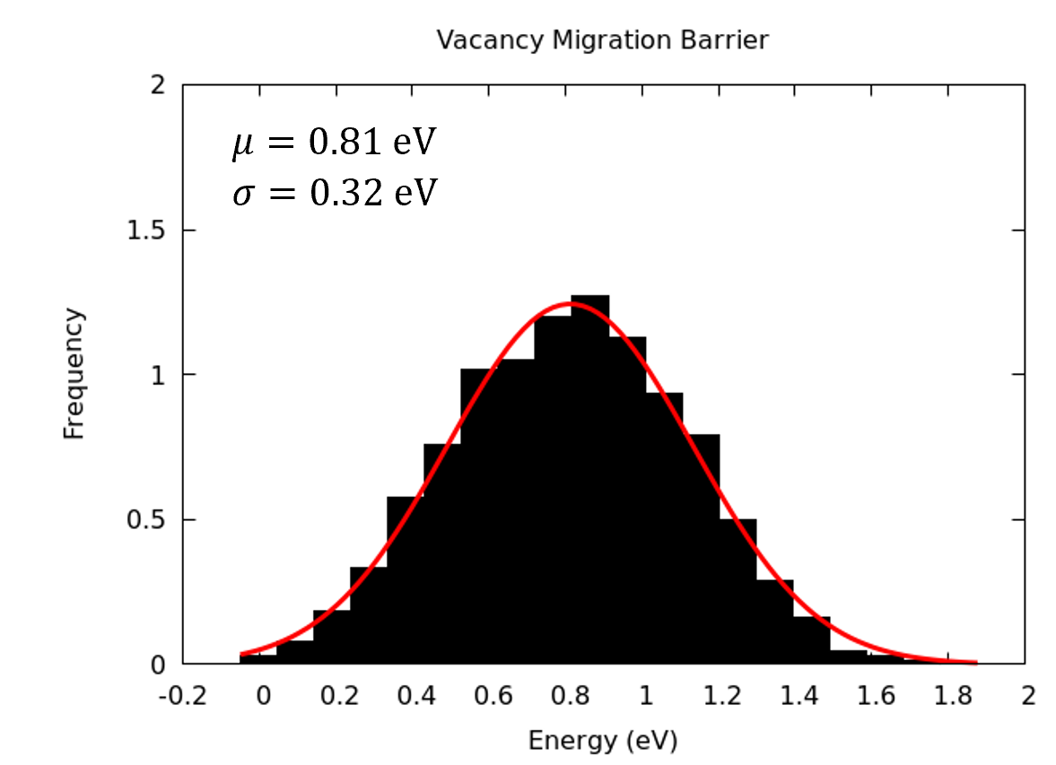
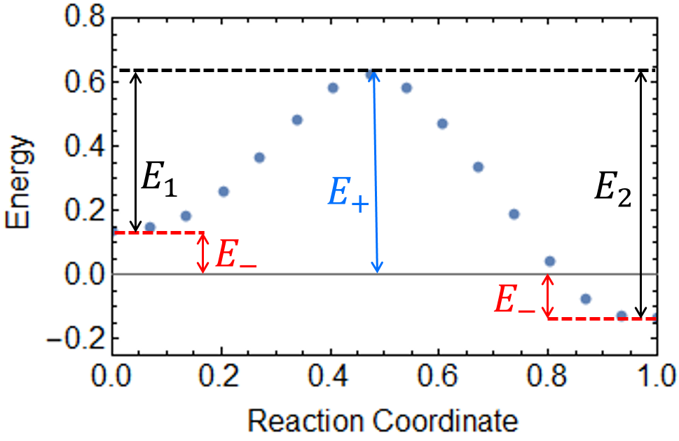
The vacancy migration barrier energies, obtained from the NEB calculations, are shown in Fig. 2. A Gaussian fit to this distribution yields a mean barrier of eV with a standard deviation of eV. The MPEA does indeed provide a rough energy landscape for vacancy migration, but to connect this to transport, we need more information than this, namely the extent to which this distribution is described by a random barrier (RB) or a random trap (RT) model. Figure 3a gives the result of one NEB calculation. The leftmost point is the energy of the initial state, the rightmost the energy of the final state. The intermediate points are the energy of mid-transition states, relaxed as the vacancy migrates, and the highest point corresponds to the saddle point of the transition.
 |
| (a) |
 |
| (b) |
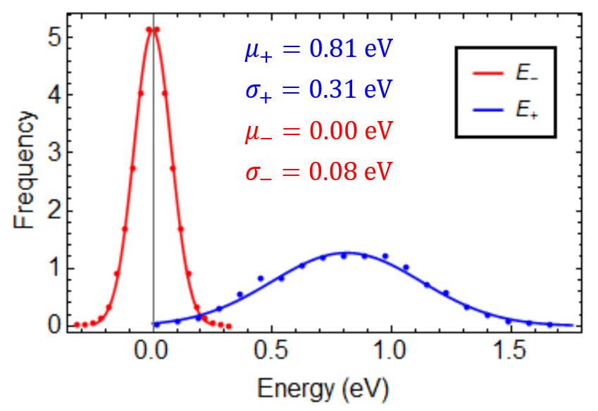
There are two primary effects of randomness in the distribution of barrier heights and well-depths. First, it affects the average transition rate. Second, it introduces correlations between subsequent hops. For example, in a purely RB model, a vacancy that just crossed a barrier with a small saddle energy is more likely to jump backwards over that same small barrier in the next hop. While the RT and RB models are constructed in terms of and , they cannot be measured directly in a useful way. In the MPEA, there is no well-defined reference energy; both the before and after a transition are equally valid reference states, and many changes in the system (such as a swap between two atoms far away from the vacancy) can shift both and without meaningfully altering the transition barrier. Instead, we consider the symmetric and anti-symmetric components of the transition, and , respectively. If we choose a reference energy equal to the mean energy between the initial and final states, then while . These are local descriptors of the transition barrier. If and are independent random variables, then the distributions of and are related to and in a predictable way (see Table 1).
| Quantity | |
|---|---|
These relationships translate from global quantities like and to local quantities that directly compare the transitions between adjacent states. Distributions of , and from the NEB calculations are given in Fig. 3b. A few initial observations can be made from this data. First, eV, is significantly greater than eV. This is more consistent with an RB-like landscape, but there is still an RT component that cannot be ignored. There are also a substantial number of transitions with very small barriers (). While states with “zero barriers” can be disregarded as unstable states, there are a large number of states that are stable, but with very small non-zero barriers. This implies a small barrier for the vacancy to hop between two sites in either direction. Intuitively, one can imagine a vacancy rapidly hopping back and forth between the two sites. As a result, we should expect highly correlated vacancy migration and a theory for diffusion in this system must account for such correlations.
These NEB calculations illustrate the nature of the energy landscape in this particular MPEA. However, it is not clear how and affect diffusion kinetics. In the next section, we present Kinetic Monte Carlo results that predict the diffusion constant as a function of and and inform the development of a theoretical model.
4 KMC Simulations
The NEB calculations provide the full distribution of transition energies and well depths in the CoNiFeCrMn MPEA. To understand the role of the distribution widths ( amd ) on the vacancy diffusivity, we performed lattice Kinetic Monte Carlo (KMC) simulations. In KMC, we can directly specify the energy landscape and control the distribution of barriers. While and are not globally independent in real systems, we can construct a model system in which they are and use the relations in Table 1 to pick and such that and follow distributions observed in NEB calculations and reflect the local character of the MPEA.
While setting up a traditional KMC simulation with a fixed distribution of and is trivial, the KMC set-up for MPEA vacancy diffusivity needs subtle, but important, modifications. These modifications are as follows:
-
1.
The energy landscape has to be dynamic. That is, one cannot a priori assign the values of and on the lattice and keep them fixed during the KMC simulation. This can be easily seen by imagining a vacancy moving in a random solid-solution. If a vacancy starts at a site , completes a few hops, and returns to its original site , such that the local atomic configuration is modified by the swapping of neighbors, then the site and barrier energies also change. Therefore, a model that accounts for this dynamic energy landscape has to be considered.
-
2.
If the local atomic configuration does not change, then the site energy remains unchanged. That is, if a local atomic environment (consider the first nearest-neighbor shell around the vacancy) remains unchanged, then the site energy should remain the same. The same is true for the transition-state energies, except that we need to consider the environments of the both the initial and the final states.
In this study, we developed an indexing approach (determined by the nearest-neighbor configuration) to guarantee that the dynamic nature and the translational symmetry of the energy landscape are satisfied. Please refer to Supplementary Information S1 for a discussion the details of the KMC simulation set-up. It is important to mention here that our indexing approach does not satisfy invariance with respect to rotation/inversion symmetries. However, we do not anticipate this to change the results significantly because we are using a statistical model. By not considering the rotation/inversion symmetries, we simply add to the diversity of the configurations. As we keep the underlying distributions the same, adding the rotation/inversion symmetries would be computationally very expensive while not altering the results significantly.
Once the transition rates are calculated according to the and arrays, the simulation proceeds via the Bortz-Kalos-Lebowitz algorithm [bortz1975new]. For each transition from a site , the rate is
| (1) |
where is an attempt frequency, is the migration barrier, and a transition is chosen randomly with a probability proportional to its rate. The vacancy site is then occupied by the target neighbor atomic species and the neighbor is then occupied by the vacancy and the time is incremented by
| (2) |
where is the sum of all transition rates and is a number chosen from a uniform distribution . This process is repeated for each step of the simulation. The diffusion constant can then be computed by measuring the mean-square displacement as a function of time, averaged over many runs of the simulation (i.e., ).
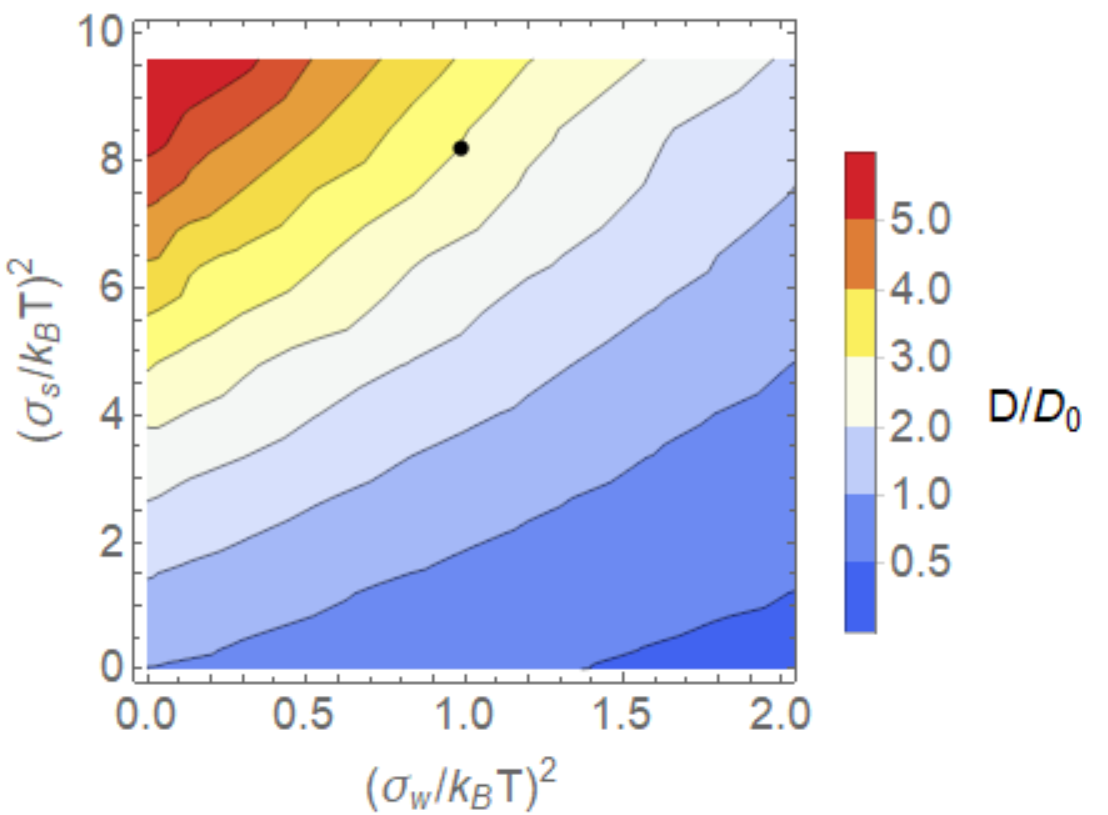
The results of KMC simulations at a fixed temperature and mean barrier eV (corresponding to the NEB measurements) over a range of and are given in Fig. 4. It is immediately apparent that while diffusivity decreases with increasing , it increases with increasing . For and chosen to match and for the CoNiFeCrMn MPEA, one would expect approximately a three-fold enhancement in vacancy diffusivity relative to a material with a uniform barrier distribution. This makes intuitive sense; for a random trap model (large ), the time is dominated by the vacancy’s residence in deep energy wells. For a random barrier model, large barriers do not impede migration of the vacancy if there are alternative short barriers that it can traverse instead.
This can be understood by analogy to resistors. For a random trap model, the roughness in the potential corresponds to a variation between subsequent hops; the total resistance of a series of resistors is given by the sum of resistances, which is dominated by the largest resistances. For a random barrier model, the roughness in the potential corresponds to a variation between alternate transitions out of a given state; the resistance of a set of resistors in parallel is given by the inverse of the sum of conductivities, for which small resistances dominate. One cannot decrease resistance by adding a weak resistor in series no more than one can increase the resistance by adding a strong resistor in parallel. To fully explain these results and make future predictions, we next present a statistical theory of vacancy migration in disordered energy landscapes.
5 Theory
The KMC simulations provide the foundational observation that random trap landscapes impede diffusion while random barrier landscapes enhance it. An analytical theory is necessary to explain these observations and make intuitive predictions. A rough energy landscape can have two effects on diffusion. First, it can change the average transition rate (analogous to the effective rates computed in prior work [zwanzig1988diffusion, mussawisade1997combination, banerjee2014diffusion, seki2015relationship, seki2016anomalous]). Second, it can introduce correlations between hops. Consider a rough landscape given by random, independent distributions of well-energies and transition saddle-point-energies , with means and and standard deviations and . The diffusion constant can be expressed as
| (3) |
where and are the diffusion constant and jump frequency for a random walker in a landscape with constant vacancy migration barrier energy and is the effect of correlations. When the vacancy migration barrier is a constant value, there are no correlations and . It is important to note that depends only on the distribution of saddle-point energies and not on the distribution of well-energies. That is, for a purely random trap energy landscape . This is because is the property of the lattice site and all jumps out of that site are equally likely (refer to Figure 1(a)). Therefore, the randomness in the well-energies will not affect which transition is selected and hence cannot influence correlations between subsequent hops. Therefore, we omit the dependence of for in equation 3. In the following, we will derive the analytical form for the jump frequency and the effect of correlations in the disordered energy landscape. The derivation will include the following steps:
-
1.
First, we will show that the contributions of the disorder in well-energies can be separated from those in the saddle-point energies. That is, the mixed model can be simplified into two independent contributions arising from a pure random-trap and a pure random-barrier model.
-
2.
The random trap contribution is equivalent to the expression derived by Zwanzig [zwanzig1988diffusion]. For the random-barrier contribution, we outline the steps required to compute the average transition rate for a random barrier model. The key insight that we will develop here is that the distribution of barriers-crossed (hops) is not the same as the distribution of barriers present in the system.
-
3.
Finally, we derive the effect of correlations in the random barrier model. As the well-energy distributions do not contribute to (as discussed above), it suffices to simply compute the correlations for the pure RB model.
5.1 Separation of the random trap (RT) and random barrier (RB) contributions
Assuming vacancy migration is thermally-activated with an attempt frequency , the rate of a transition, from state to , is given by , where . The average time that a vacancy resides in state is therefore
| (4) |
where is the coordination number and the number of possible jumps for the vacancy. If and are independent random variables, their corresponding terms can be separated. That is,
| (5) |
The average is over all hops (i.e,. all chosen transitions), rather than all possible transitions. As the choice of a transition is independent of , an average over encountered by the vacancy is simply the system-wide normal distribution of and the Arrhenius part of the RT component is
| (6) |
identical to Zwanzig’s result [zwanzig1988diffusion]. Here, we introduce the symbol for the Arrhenius part of the jump frequency. The remaining RB component,
| (7) |
is independent of . That is, we can solve the case of the mixed energy model as independent contributions of a pure random-trap model, (Eq. 6), and a pure random-barrier model (Eq. 7), that is .
5.2 Computing the jump frequency for a pure random-barrier model
To compute the arrhenius part, in equation 7, we have to determine the distribution of the barriers crossed by the vacancy in the random-walk trajectory. This is different from the distribution of the barriers present in the system as the vacancy prefers to jump over smaller barriers. For a uniform landscape, where the migration energy barrier is given by and , the Arrhenius parts of the jump frequency are given by and . The jump frequency, in the uniform barrier case, has the form . That is, while and are sensitive to the choice of reference energies (e.g., choosing or ), the product is not. In the disordered energy landscape, is independent of the distribution of well-energies, , and it can be calculated by fixing to a constant value, i.e. . For clarity, we choose a reference energy such that and and adopt a reduced notation , , and . is drawn from a truncated normal distribution:
| (8) |
over the domain . is a normalization constant. From a given lattice site, the probability of selecting a given transition is
| (9) |
where is the barrier of the target transition and represent all of the other transition barriers.
If the vacancy jumps over a small barrier , it is likely to hop backwards across that same barrier (for the random-barrier energy landscape). This means that the distribution of encountered by the vacancy should be biased towards smaller barriers relative to the system-wide barrier distribution, . The distribution of chosen barriers is
| (10) |
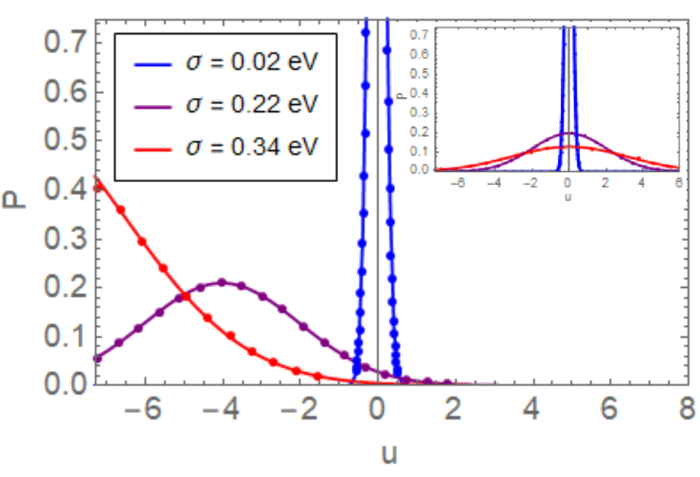
where is a normalization constant. Equation 10 can be understood as follows: the probability that a barrier first encountered by the vacancy has height is given by (equation 8). The probability of the vacancy crossing that barrier once is given by (equation 9), crossing twice is given by , etc. The sum of these probabilities is then . This distribution (with inset), compared with KMC results, is shown in Fig. 5. The distribution is nearly identical to the KMC results.
The Arrhenius part of the random barrier model, , is related to the inverse of the average of residence times (as shown in equation 7). That is, the jump frequency for the RB model can be expressed as where . Here the residence time, of the vacancy in the lattice-site is given by:
| (11) |
where is the saddle-point energy for the hop from state to state . Suppose the vacancy arrives at state by hopping over a barrier given by the non-dimensionalized variable . The barriers that the vacancy now observes, from state , are and (). We use two different variables and to denote the barriers from state to emphasize the fact that they are drawn from two distinct probability distributions. Since the vacancy just hopped over the barrier , the corresponding distribution is given by (equation 10. The distributions of the remaining barriers, defined by random variables , correspond to the system-wide function, (equation 8). The residence time, , can be re-written in-terms of the the non-dimensional variables, and , as:
| (12) |
The mean of the residence times, , can be obtained by a twelve-fold integral of the rate terms, and , multiplied by the appropriate distribution functions, and , respectively. Unfortunately, there are no analytical solutions for the integration of the rate terms, , when the random variable is described by a truncated normal distribution.
Instead, we introduce approximate probability distributions for the summation of rates, defined using the variable , where is a random variable drawn from a truncated normal distribution. is now a random variable, defined as the sum of rates over barriers, with a probability distribution . The determination of the distributions, , is described in Supplementary Information S2. Equipped with the distribution functions, , we can now simplify the computation of the average residence time . The residence time, for site , can be re-written as and the average residence time can simply be computed as a two-fold integral over the random variables and , multiplied by the appropriate distribution functions and , respectively. Therefore, the Arrhenius part, , can be written in terms of a two-fold integral as:
| (13) |
which can be evaluated numerically. As mentioned above, the barrier that the vacancy most recently hopped is drawn from the distribution (Figure 5). As favors smaller barriers, the average rate in the model will be higher than that for a uniform distribution. This also implies correlations between subsequent hops - if the vacancy hops over a particularly short barrier, it is more likely to hop backwards in the direction opposite the previous hop.
5.3 Computing the correlation factor between hops
The th correlation factor is the average cosine between a given hop and hops subsequent. If the hops are completely uncorrelated, then . In a vein similar to the derivation of the , we will suppose that a vacancy reaches site by hopping over a barrier . Let us also denote the barrier over a hop in the same direction as the previous jump as . Then the average cosine for the next hop from site is given by:
| (14) |
where is the sum of the rate terms of the remaining barriers, i.e. . This expression can be rationalized as follows: (i) the term reflects the possibility that the vacancy hops backwards over the same barrier (corresponding to a cosine of ), (ii) the term corresponds to a hop in the same direction as the previous hop (corresponding to a cosine of ), and on average, the cosine terms of all other hops cancel out in the numerator. (iii) In the denominator, we have the summation of the probabilities of all possible jumps, given by , and (for the remaining jumps). As discussed in Supplementary Information S2, is a random-variable whose distribution is given by the function .
The first correlation factor is then obtained by integrating over the distributions , and as:
| (15) |
where
| (16) |
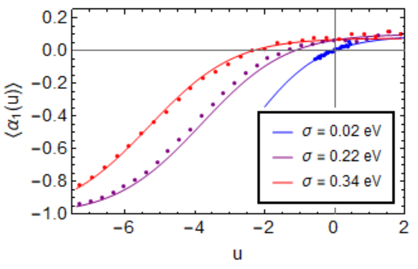
These integrals can be easily evaluated using numerical integration techniques. In Figure 6(a), we plot the marginal distribution defined as:
| (17) |
Shown in Figure 6(a), is a close match between and the KMC simulations for three different values of . Note the convergence of to as decreases. For smaller barriers , it is very highly likely that the vacancy will jump back over that small barrier. This results in an angle of 180∘ between subsequent hops and the average cosine will converge to -1.
 |
| (a) |
 |
| (b) Correlation Factors |
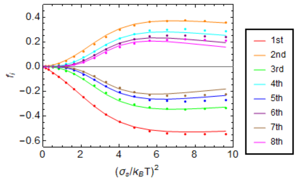
For higher order correlations (i.e., the correlation between a hop and the th subsequent hop), one must determine corresponding terms (see Supplementary Information 3). The first eight correlation factors () are plotted in Fig. 6b, compared directly with measurements from KMC simulations. The theory is nearly an exact match to the simulations, except for the high-order correlation factors at large . This is discussed further in Supplementary Information S3. The effect of correlation factors on the diffusion coefficient, up to the n correlation factor, is given by
| (18) |
This is a modification of the common random walker solution with correlated hops for finite sums [shewmon2016diffusion]; if, for example, we consider up to the 8th correlation factor, then we sample from an initial hop up to 9 hops in the future. This means that 8 instances of count toward the average, 7 instances of , etc. We note here that it is common in the theory of correlated random walks to approximate [shewmon2016diffusion]; this is only valid if every state is equivalent, such that . That is not true in this case, as evidenced by Fig. 6.
6 Results and Discussion
The analytical diffusivity (the ratio , where is the diffusivity when ) is plotted as a function of and in Fig. 7a, and the error between the theory and KMC is given in Fig. 7b. The theory and KMC produce nearly identical results, except when both and are large. This is because while the random barrier model does not allow the component of transition energy to be less than , it does not account for the effect of particularly deep wells, which could allow stable configurations where as long as . This is, however, only a problem when and/or are much greater than measured for the CoNiFeCrMn HEA.
 |
| (a) Random-Walk Theory |
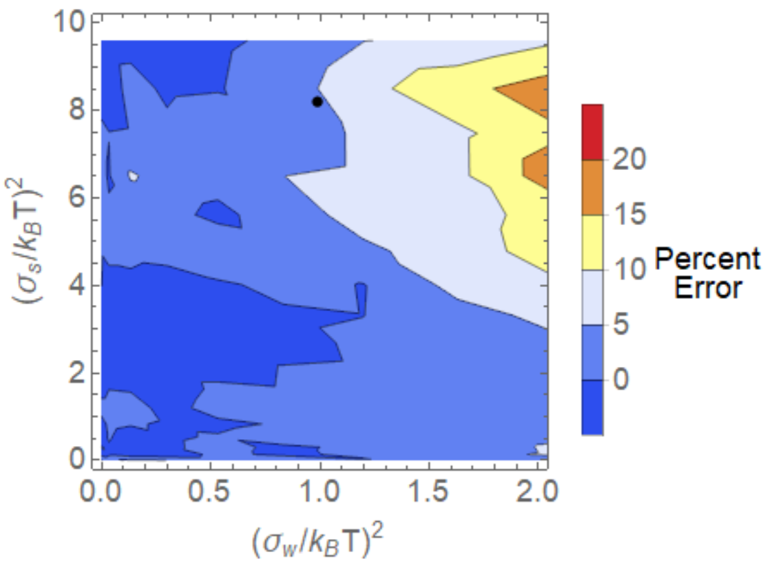 |
| (b) Error |
These plots show that vacancy diffusivity can either be retarded ( if and ) or accelerated ( if and ) depending on the widths of the distributions of site energies and transition-state energies . This captures the full breadth of behaviors observed in more recent experimental results, while perhaps explaining the assumed universality of sluggish diffusion in MPEAs. The KMC simulations and theoretical model presented here provide insight to the relationship between the energy landscape and the resulting transport properties. In the most general terms, a large (or ) yields enhanced diffusion, while a large (or ) produces sluggish diffusion. Diffusion constants may be difficult to measure directly, but the method presented here, to compute and distributions, is amenable to automated survey that can be used to probe the high-dimensional compositional space of MPEAs.
The model also allows us to directly quantify the influence of correlations between hops and barrier selection on diffusion in a random energy landscape. Figure 8 shows a comparison between KMC and Theory for the pure random barrier model and a simplified model. In the simplified KMC, all transitions from a given state are given equal probability , irrespective of the barrier energy, at each time step. In the simplified theory, we equate the probability of hopped barriers to the system-wide distribution of transition state energies, i.e. . Under these conditions, the averaging over all chosen vacancy hops (Eq. 7) can be computed by simply averaging over the entire energy landscape, making it more similar to the Effective Medium approximation common in existing literature [webman1981effective, ansari1985protein, haus1987diffusion, ambaye1995asymptotic, mussawisade1997combination, seki2016anomalous]. The two cases are very similar due to the competing effects of preferential small-barrier selection and hop correlation. For example, when eV, is approximately times larger than in the equal-probability case but the correlation factor . Therefore, the difference between the two scenarios (as shown in Figure 8) is not very large. However, this is not guaranteed for different temperatures and mean barriers. It is important to identify the correct theory for modeling the random energy landscape if we wish to accurately model diffusion in disordered materials.
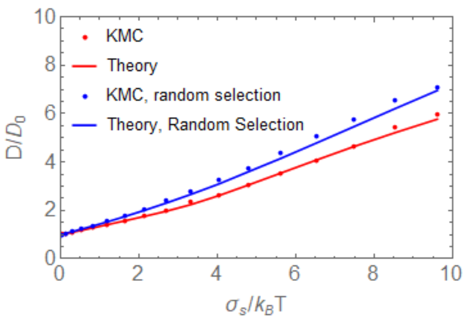
Irrespective of the assumptions that went into this KMC and theoretical model, it is clear that the random barrier/trap character of the energy landscape can profoundly influence diffusion, potentially altering the effective diffusion constant by at least an order of magnitude; these details are necessary to predict diffusion behaviors in disordered systems and must be considered in future models.
7 Conclusions
The set of experimentally synthesized alloys cover only a small region of the high-dimensional compositional space that has been identified as thermodynamically plausible for MPEAs [senkov2015accelerated, miracle2017critical]. To sample this high-dimensional space in an efficient manner and to design novel MPEAs with targeted properties, the need for new theoretical and computational tools has been highlighted [george2019high]. In this current study, we focused on developing analytical tools for predicting diffusion kinetics, which are time consuming to measure either using experiments or atomistic simulations. For diffusivity in MPEAs, the computational tools require a foundation of a) characterization of the kinetic barriers to diffusion, b) a means of simulating diffusion in a model system faithful to the observed energy landscape, and c) a theoretical framework for understanding how the underlying energy landscape relates to diffusion.
In this article, we presented a complete cross-section of diffusion in rough energy landscapes, where the disorder is representative of solid-solution MPEAs. We developed a flexible KMC protocol where the distributions of the disordered well and the saddle-point energies can be independently controlled. To better understand the KMC results and to develop predictive models, we presented a theoretical framework for vacancy diffusivity in disordered energy landscapes. While the statistics used in the KMC simulations are informed by the direct computation of the migration barriers for a CoNiFeCrMn EAM potential, the developed theory spans a wide-range of distributions that one may observe in generic MPEAs. Therefore, for a given alloy system, equipped with knowledge of the well and saddle-point energy distributions, simulations and theoretical results provided in this article can be used to predict transport properties. The theory itself lends to an intuition regarding transport; wider distributions of saddle-point energies enhance diffusion while wider distributions of well depths stifle diffusion. If these distributions can be connected to alloy chemistry and compositions, designer MPEAs with optimized transport properties can be achieved.
As it stands, our model is insensitive to correlations in the energies. That is, the relationship between neighboring species and migration barriers is completely random. There is also no mixing enthalpy and no consideration for different migration barriers for different atomic species. This is significant; it has been noted, for example, that the presence of Mn is associated with sluggish diffusion in the CoNiFeCrMn MPEA [dkabrowa2019demystifying]. Our own observations suggest that Mn generally has the smallest barrier to migration, consistent with the findings of Tsai et al. [tsai2013sluggish]. This seemingly contradictory result highlights the subtle nature of this effect and the need for tools to directly measure the energy landscape and connect that to actual diffusion behavior. While our model does not address the influence of different species having different kinetics (which our NEB data does suggest), existing Onsager-type continuum and multi-frequency models [moleko1989self, druger1983dynamic, perondi1997bond, perondi1997trap, allnatt2016high, trinkle2018variational] may be used in conjunction with our method to address this. In future work, the tools presented here will be augmented appropriately to investigate these effects and guide the design of multi-principal alloy systems.
We hope that this statistical treatment of vacancy diffusion provides a building block for future navigational tools in the vast MPEA sea. In the near term, it should also serve as a guide for what computational tools currently in development must do correctly. The potential that we used [choi2018understanding] is a laudable effort - a necessary step for the atomistic modeling of these complex alloys. However, for understanding vacancy diffusivity, it is insufficient to match just the vacancy migration barriers. That is only half the information; holding that steady, one can change the diffusion constant by orders of magnitude. MPEA potentials cannot be relied upon for diffusion-related problems if they do not capture the full nature of the vacancy migration landscape - the symmetric and anti-symmetric barrier components used here may be useful quantities for measurements and fits. This necessary level of detail may also be an opportunity for novel machine learning approaches to modeling transport in MPEAs [kostiuchenko2019impact].
Acknowledgements
This work is supported by the U.S. National Science Foundation under Grant No. CMMI-1826173.
References
References
- [1] O. N. Senkov, G. Wilks, J. Scott, D. B. Miracle, Mechanical properties of Nb25Mo25Ta25W25 and V20Nb20Mo20Ta20W20 refractory high entropy alloys, Intermetallics 19 (5) (2011) 698–706.
- [2] A. Gali, E. P. George, Tensile properties of high-and medium-entropy alloys, Intermetallics 39 (2013) 74–78.
- [3] B. Gludovatz, A. Hohenwarter, D. Catoor, E. H. Chang, E. P. George, R. O. Ritchie, A fracture-resistant high-entropy alloy for cryogenic applications, Science 345 (6201) (2014) 1153–1158.
- [4] Z. Zhang, M. Mao, J. Wang, B. Gludovatz, Z. Zhang, S. X. Mao, E. P. George, Q. Yu, R. O. Ritchie, Nanoscale origins of the damage tolerance of the high-entropy alloy CrMnFeCoNi, Nature communications 6 (2015) 10143.
- [5] D.-H. Lee, M.-Y. Seok, Y. Zhao, I.-C. Choi, J. He, Z. Lu, J.-Y. Suh, U. Ramamurty, M. Kawasaki, T. G. Langdon, et al., Spherical nanoindentation creep behavior of nanocrystalline and coarse-grained CoCrFeMnNi high-entropy alloys, Acta Materialia 109 (2016) 314–322.
- [6] Y. Ma, Y. Feng, T. T. Debela, G. Peng, T. Zhang, Nanoindentation study on the creep characteristics of high-entropy alloy films: FCC versus BCC structures, International Journal of Refractory Metals and Hard Materials 54 (2016) 395–400.
- [7] L. Zhang, P. Yu, H. Cheng, H. Zhang, H. Diao, Y. Shi, B. Chen, P. Chen, R. Feng, J. Bai, et al., Nanoindentation creep behavior of an Al0.3CoCrFeNi high-entropy alloy, Metallurgical and Materials Transactions A 47 (12) (2016) 5871–5875.
- [8] T. Cao, J. Shang, J. Zhao, C. Cheng, R. Wang, H. Wang, The influence of Al elements on the structure and the creep behavior of CoCrFeNi high entropy alloys, Materials Letters 164 (2016) 344–347.
- [9] T. Egami, W. Guo, P. Rack, T. Nagase, Irradiation resistance of multicomponent alloys, Metallurgical and Materials Transactions A 45 (1) (2014) 180–183.
- [10] S.-q. Xia, W. Zhen, T.-f. Yang, Y. Zhang, Irradiation behavior in high entropy alloys, Journal of Iron and Steel Research, International 22 (10) (2015) 879–884.
- [11] S. Xia, X. Yang, T. Yang, S. Liu, Y. Zhang, Irradiation resistance in AlxCoCrFeNi high entropy alloys, Jom 67 (10) (2015) 2340–2344.
- [12] F. Granberg, K. Nordlund, M. W. Ullah, K. Jin, C. Lu, H. Bei, L. Wang, F. Djurabekova, W. Weber, Y. Zhang, Mechanism of radiation damage reduction in equiatomic multicomponent single phase alloys, Physical review letters 116 (13) (2016) 135504.
- [13] N. K. Kumar, C. Li, K. Leonard, H. Bei, S. Zinkle, Microstructural stability and mechanical behavior of FeNiMnCr high entropy alloy under ion irradiation, Acta Materialia 113 (2016) 230–244.
- [14] G. R. Holcomb, J. Tylczak, C. Carney, Oxidation of CoCrFeMnNi high entropy alloys, Jom 67 (10) (2015) 2326–2339.
- [15] W. Kai, C. Li, F. Cheng, K. Chu, R. Huang, L. Tsay, J. Kai, The oxidation behavior of an equimolar FeCoNiCrMn high-entropy alloy at 950∘C in various oxygen-containing atmospheres, Corrosion Science 108 (2016) 209–214.
- [16] G. Laplanche, U. Volkert, G. Eggeler, E. George, Oxidation behavior of the CrMnFeCoNi high-entropy alloy, Oxidation of Metals 85 (5-6) (2016) 629–645.
- [17] D. B. Miracle, High-entropy alloys: A current evaluation of founding ideas and core effects and exploring “nonlinear alloys”, Jom 69 (11) (2017) 2130–2136.
- [18] K.-Y. Tsai, M.-H. Tsai, J.-W. Yeh, Sluggish diffusion in Co–Cr–Fe–Mn–Ni high-entropy alloys, Acta Materialia 61 (13) (2013) 4887–4897.
- [19] A. Ansari, J. Berendzen, S. F. Bowne, H. Frauenfelder, I. Iben, T. B. Sauke, E. Shyamsunder, R. D. Young, Protein states and proteinquakes, Proceedings of the National Academy of Sciences 82 (15) (1985) 5000–5004.
- [20] J. W. Haus, K. W. Kehr, Diffusion in regular and disordered lattices, Physics Reports 150 (5-6) (1987) 263–406.
- [21] R. Zwanzig, Diffusion in a rough potential, Proceedings of the National Academy of Sciences 85 (7) (1988) 2029–2030.
- [22] J. Dabrowa, M. Zajusz, W. Kucza, G. Cieślak, K. Berent, T. Czeppe, T. Kulik, M. Danielewski, Demystifying the sluggish diffusion effect in high entropy alloys, Journal of Alloys and Compounds 783 (2019) 193–207.
- [23] D. Miracle, High entropy alloys as a bold step forward in alloy development, Nature communications 10 (1) (2019) 1805.
- [24] F. Zhang, C. Zhang, S.-L. Chen, J. Zhu, W.-S. Cao, U. R. Kattner, An understanding of high entropy alloys from phase diagram calculations, Calphad 45 (2014) 1–10.
- [25] C.-Y. Cheng, J.-W. Yeh, High thermal stability of the amorphous structure of NbTaTiZr (x=0.5, 1) high-entropy alloys, Materials Letters 181 (2016) 223–226.
- [26] C.-Y. Cheng, J.-W. Yeh, High-entropy BNbTaTiZr thin film with excellent thermal stability of amorphous structure and its electrical properties, Materials Letters 185 (2016) 456–459.
- [27] Y. Zhao, H. Chen, Z. Lu, T. Nieh, Thermal stability and coarsening of coherent particles in a precipitation-hardened (NiCoFeCr)94Ti2Al4 high-entropy alloy, Acta Materialia 147 (2018) 184–194.
- [28] P. Kumar, S. Avasthi, Diffusion barrier with 30-fold improved performance using AlCrTaTiZrN high-entropy alloy, Journal of Alloys and Compounds 814 (2020) 151755.
- [29] S. Praveen, H. S. Kim, High-entropy alloys: Potential candidates for high-temperature applications–an overview, Advanced Engineering Materials 20 (1) (2018) 1700645.
- [30] Y. Lu, H. Huang, X. Gao, C. Ren, J. Gao, H. Zhang, S. Zheng, Q. Jin, Y. Zhao, C. Lu, et al., A promising new class of irradiation tolerant materials: Ti2ZrHfV0.5Mo0.2 high-entropy alloy, Journal of materials science & technology 35 (3) (2019) 369–373.
- [31] C. M. Barr, J. E. Nathaniel II, K. A. Unocic, J. Liu, Y. Zhang, Y. Wang, M. L. Taheri, Exploring radiation induced segregation mechanisms at grain boundaries in equiatomic CoCrFeNiMn high entropy alloy under heavy ion irradiation, Scripta Materialia 156 (2018) 80–84.
- [32] H. Jeong, H. Park, K. Park, T. Na, W. Kim, High-temperature deformation mechanisms and processing maps of equiatomic CoCrFeMnNi high-entropy alloy, Materials Science and Engineering: A 756 (2019) 528–537.
- [33] R. W. Balluffi, S. M. Allen, W. C. Carter, Kinetics of materials, John Wiley & Sons, 2005.
- [34] L. Moleko, A. Allnatt, E. Allnatt, A self-consistent theory of matter transport in a random lattice gas and some simulation results, Philosophical Magazine A 59 (1) (1989) 141–160.
- [35] A. Allnatt, T. Paul, I. Belova, G. Murch, A high accuracy diffusion kinetics formalism for random multicomponent alloys: application to high entropy alloys, Philosophical Magazine 96 (28) (2016) 2969–2985.
- [36] D. R. Trinkle, Variational principle for mass transport, Physical review letters 121 (23) (2018) 235901.
- [37] S. Summerfield, Effective medium theory of AC hopping conductivity for random-bond lattice models, Solid State Communications 39 (3) (1981) 401–402.
- [38] T. Odagaki, M. Lax, Coherent-medium approximation in the stochastic transport theory of random media, Physical Review B 24 (9) (1981) 5284.
- [39] I. Webman, Effective-medium approximation for diffusion on a random lattice, Physical Review Letters 47 (21) (1981) 1496.
- [40] S. Banerjee, R. Biswas, K. Seki, B. Bagchi, Diffusion on a rugged energy landscape with spatial correlations, The Journal of chemical physics 141 (12) (2014) 124105.
- [41] K. Seki, B. Bagchi, Relationship between entropy and diffusion: A statistical mechanical derivation of rosenfeld expression for a rugged energy landscape, The Journal of chemical physics 143 (19) (2015) 194110.
- [42] K. Seki, K. Bagchi, B. Bagchi, Anomalous dimensionality dependence of diffusion in a rugged energy landscape: How pathological is one dimension?, The Journal of chemical physics 144 (19) (2016) 194106.
- [43] Y. N. Osetsky, L. K. Béland, R. E. Stoller, Specific features of defect and mass transport in concentrated FCC alloys, Acta Materialia 115 (2016) 364–371.
- [44] K. Mussawisade, T. Wichmann, K. Kehr, Combination of random-barrier and random-trap models, Journal of Physics: Condensed Matter 9 (6) (1997) 1181.
- [45] H. Ambaye, K. W. Kehr, Asymptotic diffusion coefficient of particles in a random medium, Physical Review E 51 (5) (1995) 5101.
- [46] G. Henkelman, B. P. Uberuaga, H. Jónsson, A climbing image nudged elastic band method for finding saddle points and minimum energy paths, The Journal of chemical physics 113 (22) (2000) 9901–9904.
- [47] G. Henkelman, H. Jónsson, Improved tangent estimate in the nudged elastic band method for finding minimum energy paths and saddle points, The Journal of chemical physics 113 (22) (2000) 9978–9985.
- [48] A. Nakano, A space–time-ensemble parallel nudged elastic band algorithm for molecular kinetics simulation, Computer Physics Communications 178 (4) (2008) 280–289.
- [49] E. Maras, O. Trushin, A. Stukowski, T. Ala-Nissila, H. Jonsson, Global transition path search for dislocation formation in Ge on Si (001), Computer Physics Communications 205 (2016) 13–21.
- [50] W.-M. Choi, Y. H. Jo, S. S. Sohn, S. Lee, B.-J. Lee, Understanding the physical metallurgy of the CoCrFeMnNi high-entropy alloy: an atomistic simulation study, npj Computational Materials 4 (1) (2018) 1.
- [51] S. Plimpton, Fast parallel algorithms for short-range molecular dynamics, Journal of computational physics 117 (1) (1995) 1–19.
- [52] B. Sadigh, P. Erhart, A. Stukowski, A. Caro, E. Martinez, L. Zepeda-Ruiz, Scalable parallel monte carlo algorithm for atomistic simulations of precipitation in alloys, Physical Review B 85 (18) (2012) 184203.
- [53] E. Bitzek, P. Koskinen, F. Gähler, M. Moseler, P. Gumbsch, Structural relaxation made simple, Physical review letters 97 (17) (2006) 170201.
- [54] D. Sheppard, R. Terrell, G. Henkelman, Optimization methods for finding minimum energy paths, The Journal of chemical physics 128 (13) (2008) 134106.
- [55] A. Fernández-Caballero, J. Wróbel, P. Mummery, D. Nguyen-Manh, Short-range order in high entropy alloys: Theoretical formulation and application to Mo-Nb-Ta-VW system, Journal of Phase Equilibria and Diffusion 38 (4) (2017) 391–403.
- [56] A. B. Bortz, M. H. Kalos, J. L. Lebowitz, A new algorithm for monte carlo simulation of ising spin systems, Journal of Computational Physics 17 (1) (1975) 10–18.
- [57] P. Shewmon, Diffusion in solids, Springer, 2016.
- [58] O. Senkov, J. Miller, D. Miracle, C. Woodward, Accelerated exploration of multi-principal element alloys with solid solution phases, Nature communications 6 (2015) 6529.
- [59] D. B. Miracle, O. N. Senkov, A critical review of high entropy alloys and related concepts, Acta Materialia 122 (2017) 448–511.
- [60] E. P. George, D. Raabe, R. O. Ritchie, High-entropy alloys, Nature Reviews Materials (2019) 1.
- [61] S. D. Druger, A. Nitzan, M. A. Ratner, Dynamic bond percolation theory: A microscopic model for diffusion in dynamically disordered systems. I. definition and one-dimensional case, The Journal of chemical physics 79 (6) (1983) 3133–3142.
- [62] L. Perondi, R. Elliott, K. Kaski, I. tracer diffusion in bond-disordered square lattices, Journal of Physics: Condensed Matter 9 (38) (1997) 7933.
- [63] L. Perondi, R. Elliott, K. Kaski, II. tracer diffusion in a system with randomly distributed traps, Journal of Physics: Condensed Matter 9 (38) (1997) 7949.
- [64] T. Kostiuchenko, F. Körmann, J. Neugebauer, A. Shapeev, Impact of lattice relaxations on phase transitions in a high-entropy alloy studied by machine-learning potentials, npj Computational Materials 5 (1) (2019) 1–7.
- [65] L. Fenton, The sum of log-normal probability distributions in scatter transmission systems, IRE Transactions on Communications Systems 8 (1) (1960) 57–67.
S1 KMC Details
For the initial configuration, we generate an FCC lattice of sites, randomly populated with one of five atomic species. One site is populated with a vacancy. The rejection-free Kinetic Monte Carlo algorithm we use is standard [bortz1975new]. However, the choice of saddle points and well-depths for transitions must be done carefully and efficiently. We chose our algorithm to satisfy the following constraints:
-
1.
Translational symmetry: the same set of nearest neighbors results in the same barriers, regardless of where it is in absolute space.
-
2.
Well-sampled barriers: many different barriers are represented and there are few identical barriers except via translational symmetry.
-
3.
Zero mixing enthalpy: no species are preferential neighbors. This term could be added subsequently to introduce short-range order, but this effect should be independently controllable.
The requirement of translational symmetry is satisfied if the barriers are a function of the nearest neighbor environment. Good sampling, as well as the zero mixing enthalpy requirement imply that bond models, or simply counting the number of neighbors of each species of the vacancy, would be insufficient. Additionally, the saddle point should be:
-
1.
Symmetric: the transition saddle-point energy from configuration A to configuration B should be the same as the energy from B to A.
-
2.
Uncorrelated: the saddle point energies of transitions from a given state should be independent - such correlations could be introduced in future work, but this should be independently controllable.
To satisfy these conditions, we initially generate random arrays of saddle heights and well depths with corresponding distribution widths and , as well as mean barrier heights and ( is chosen as zero and is chosen as , as the reference energy does not matter). If or , they are rejected and a new energy is generated randomly from the normal distribution. This is to prevent the frequent drawing of unphysical negative transition barriers. As long as and are sufficiently smaller than the difference between and , this has a negligible effect on the simulation.
At each KMC step, the species of sites neighboring the vacancy site A are used to generate an index for accessing the array (i.e., is the same for every transition out of a given state). For the -index , we consider only the nearest neighbors of the vacancy site:
| (19) |
where is the number of different species and is the type of a given neighbor (numbered from 0 to ; for the CoNiFeCrMn alloy, we choose 0 for cobalt, 1 for nickel, etc.). Here, the neighbors are sorted such that the neighbor from the central atom is always the neighbor, always the , etc. Every possible configuration of neighbor species generates a different index.
A separate index, , is determined to reference for each of the z transitions available to the vacancy (corresponding to the nearest-neighbor sites). is computed using the neighbors of both the vacancy site A and the destination site B:
| (20) |
where is the number of common neighbors between any two pairs of neighbors (4 for FCC, making for 20 total terms, including the origin and destination site). We take the modulo because would otherwise occupy a very large range from 0 to approximately , most of which would never be realized. In the interest of computational efficiency (and to prevent integer overflow), we take the modulo , where . This choice of is large and coprime with , minimizing the number of overlapping indices. The summation terms can be pre-calculated and stored in a array, removing the need for unnecessary computation. To enforce the transition-reversal symmetry of the term, this index is computed for the forward and reverse transition and the indices are added together to produce the final index used to access the array.
It should be noted that this formulation lacks any rotation/mirror/inversion symmetries. Each neighbor is unique with respect to the lab frame; shifting all atomic species and the vacancy one site over will preserve the transition barriers, but rotating all species around the vacancy will not. This sacrifice saves substantial computing time as it allows each neighbor configuration to map to an array index. Due to the disordered random nature of the transition barriers and the size of the neighbor configuration space, we do not expect this to influence the kinetics in any meaningful way. However, the effect of rotational/inversion symmetry could be a subject of further inquiry.
S2 Determination of distributions of the sum of transition rates
In the analytical theory, we are often tasked with computing the sum of multiple independent, randomly-distributed rates (e.g., Eqs. 9, 14, 15, and 16). In theory, one could integrate over these variables independently, but this would entail a 12-fold integral that is difficult and expensive to evaluate. To simplify these calculations, we computed an effective distribution of transition rates corresponding to these sums.
The exponential of a normally-distributed random variable is log-normally distributed. Unfortunately, there is no analytical solution to a sum of log-normally distributed variables. One common approximation is the Fenton-Wilkinson approximation [fenton1960sum], which assumes that the distribution of a sum of log-normally distributed independent random variables is log-normally distributed, with a mean and variance equal to the sum of the mean and variance of the summed variables. This does not apply in our case as our distributions are truncated at a zero energy barrier, but we can apply the same idea. Consider a (truncated) normal distribution of reduced energy barriers (Eq. 8),
| (21) |
where . We can compute a distribution of rates for :
| (22) | ||||
noting that this distribution ranges from 0 to 1, as ranges from to . From this distribution, we can compute the mean , variance , and third central moment of the rate distribution:
| (23) | ||||
| (24) | ||||
| (25) |
Direct measurement shows that the sum over rates resembles a lognormal distribution within the range , but then rapidly decays for . To model this, we use the piecewise function:
| (26) |
which, by definition, is continuous over the range to and converges to at large . is a normalization constant and gives the rate of decay for the tail. Note that in reality the sum of rates should be bound to the range to , but the difference is negligible because is extremely rare. and can be thought of as effective and values for an effective barrier that must be computed. To do this, we compute the mean , variance , and third central moment of this modified distribution. These integrals can be solved analytically, though the resulting expressions are cumbersome.
To compute , , and , we use the fact that , , and . These simultaneous expressions can be solved numerically for given values of , , , and z without need for curve fitting or any prior simulation. distributions, compared with numerical simulation (computed by randomly generating sets of energies according to distributions and adding the corresponding rates) are given in Fig. S1. Distributions like these were used for the effective rate terms in the primary text. Alternatively, one could numerically generate these rate sums and use fits for practical use, but this method is more readily applicable.
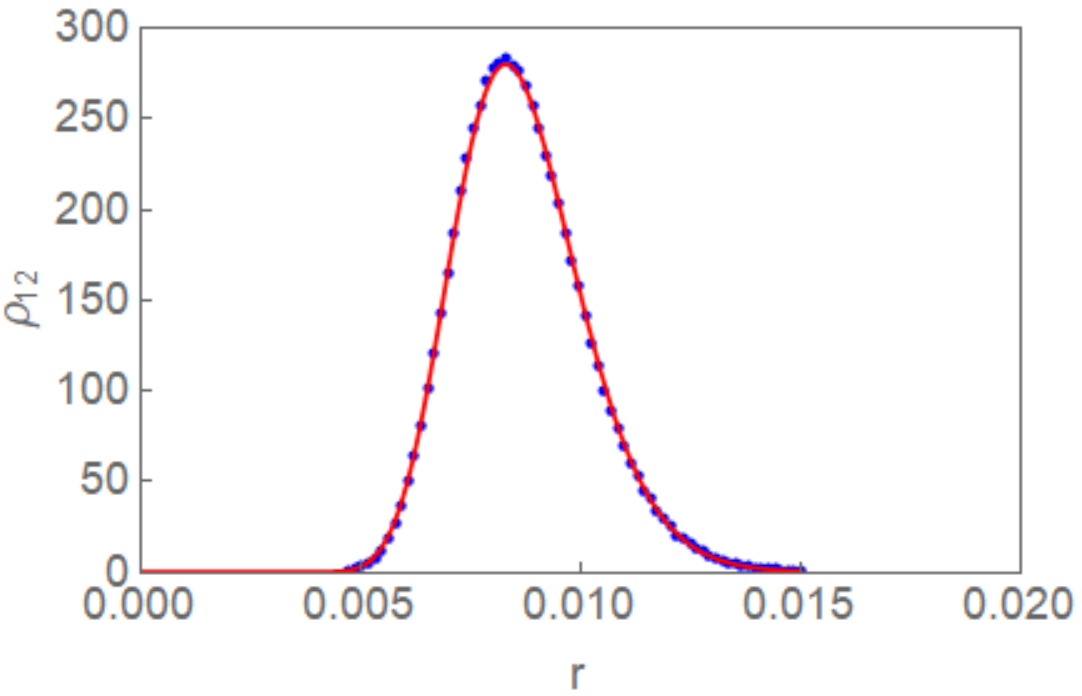 |
| (a) , eV |
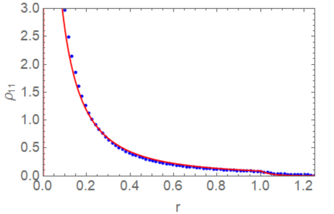 |
| (b) , eV |
S3 Higher-order correlation factors
The correlation between subsequent hops is an essential factor in the computation of the diffusion constant. The introduction of random barriers introduces correlations because a vacancy that just hopped over a small barrier is more likely to hop back again over that same barrier. The correlation factor represents , or the average cosine of the angle between a given hop and hops subsequent. The first correlation factor was given in Eq. 15 of the primary text:
| (27) |
where
| (28) |
This can be interpreted as a Boltzmann sum with the term representing the chance that the vacancy hops in the same direction as the previous hop ( ), the term representing the chance that the vacancy hops backwards over the previously-hopped barrier ( ), and the term representing the sum of the rates of other potential hops, which cancel in the numerator, but still contribute to the partition function (this fact, as well as being strongly biased toward small at large , explains why the approximations for are sufficient). For the other terms, we make the following assumptions:
-
1.
A given hop, characterized by a barrier , is only correlated with hops from the two sites that share that transition (i.e., the site occupied by the vacancy at time and the site occupied previously)
-
2.
Any hops that rearrange atomic species will randomly change the barriers, breaking the correlation
The above assumptions are true if the saddle points themselves are independent from each other(as in the KMC) and greatly reduce the number of trajectories we must consider. Figure S2 illustrates the environment around the vacancy and some of these trajectories. Any trajectories for which the last hop is from a U site do not contribute to the correlation factor, as assumption 1 dictates that all barriers around those sites are random and uncorrelated, meaning that the vacancy has an equal probability of hopping in any direction.
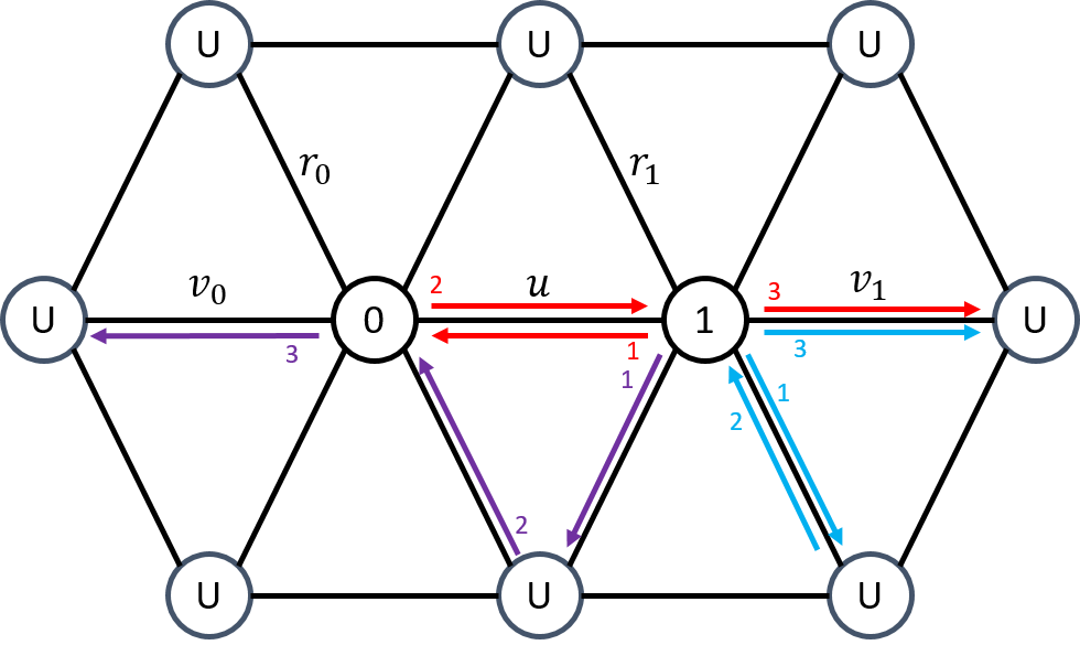
Given a set of barriers and rates corresponding to sites 0 and 1, one can compute by adding the cosine between the previous hop and the final hop of all -length trajectories (1 if parallel, -1 if anti-parallel, 0 by symmetry in all other cases), weighted by their probability. For example,
| (29) |
where the first term is the probability that the vacancy initially hops to site and the second is analogous to , but originating at site 0. The second correlation factor is then
| (30) |
The only set of trajectories that contribute to are the ones that start with a hop from 1 to 0. We will represent this by the notation , reflecting the previous site , and all trajectories that begin with a hop from 1 to 0. While trivial now, it will be useful for the more complex trajectories needed for higher order factors. For example, a trajectory can include a hop from site 0 or 1 to a U site, followed by a hop immediately back ( or ) and still contribute to the correlation factor (e.g., the blue trajectory in Fig. S2). A trajectory with a hop from 1 to U, then to 0 or vice-versa can contribute to the correlation factor if the U site is a common neighbor of 1 and 0 and both the U site and final destination site initially have the same atomic species ( probability in an -component equiatomic alloy, see the purple trajectory in Fig. S2). If they share the same atomic species then after the two hops, the nearest neighbor environments are the same as a simple 01 hop.
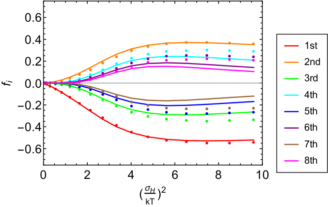
The simplest case for computing higher-order correlation factors is to consider only trajectories that involve direct back-and-forth hopping. In this case, odd-numbered factors end with a hop from site and even-numbered factors end with a hop from site . In this case,
| (31) |
where
| (32) |
and represent the ceiling and floor functions, respectively. is the sum of all transition rates from site 1 not explicitly given, while is the same for site 0. The first factor arises from every hop from 1 to 0, and the second is for every hop from 0 to 1. is a reflection of whether the final hop is from site 0 or site 1. The result of calculations made with this expression is given in Fig. S3 (which is exact for and ). This is a decent approximation for low-order factors or for small . However, as the CoNiFeCrMn MPEA exhibits large , it is insufficient for the alloy of interest. We must consider more complex trajectories that include U sites.
As the contributions of each trajectory to the correlation factor are additive, we can separate the integrals and treat different cases individually. At this point, it is worth considering the probability that the previous two hops were a 0U0 or 1U1 compound hop:
| (33) |
is, again, the 01 barrier; in this case, represents the particular barrier between 0 or 1 and the site to which the vacancy bounces, while is the effective rates of all other sites from 0 or 1 and is the effective barrier of all other sites from U. The prefactor arises simply because there are U sites neighboring 1 or 0 in an FCC system. The square in the first integrand factor reflects the fact that among the 11 other neighbors, is more likely to be a small barrier and is more likely to result in a hop back to or . This biased distribution is analogous to the distribution, except without an infinite sum it lacks an analytical normalization, hence the normalization term in the denominator. 1U0/0U1 hops do not require this biased distribution, but are only possible via the 4 U sites common to both 1 and 0. They also only contribute to the correlation factor if the U site and the final destination site have the same atomic species ( chance for an -component equiatomic alloy):
| (34) |
Equations 33 and 34 are compared with KMC results in Fig. S4. For large , approaches nearly when eV. For comparison, a 101 hop has a chance, meaning that when is large, the vacancy has a nearly chance of revisiting the site occupied 2 hops prior. This extremely high level of correlation between hops necessitates this higher-order analysis.
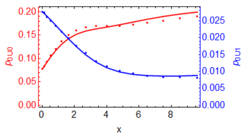
We can use these terms to make a higher-order correction to with some final approximations. We will only consider trajectories that contain a single 0U0, 1U1, 0U1, or 1U0 hop (as at most), and we will assume that , , and is uncorrelated with (in truth, they should be weakly correlated). If this assumption holds, we can use the averaged and computed above. With these assumptions in place, what is the effect of a 1U1, 0U0, or 1U0 hop? A trajectory with a or hop is identical to a trajectory without, but with 2 fewer hops. A or hop is the same, except the penultimate site flips between 0 and 1 (which flips the barrier in Fig. S2 from left to right of the penultimate site, effectively flipping the sign of ). The modified correlation factor for is then
| (35) |
where is the correlation factor computed only from hops between sites 1 and 0 (Fig. S3). The term is simply a count of the number of ways to arrange hops between 0 and 1 with one 0U0/1U1/0U1/1U0 hop. The corrected results given by Eq. 35 are given by Fig. 6b of the primary text and Fig. S5 here.
