Provably Efficient Exploration for Reinforcement Learning Using Unsupervised Learning

Fei Feng University of California, Los Angeles fei.feng@math.ucla.edu &Ruosong Wang Carnegie Mellon University ruosongw@andrew.cmu.edu &Wotao Yin University of California, Los Angeles wotaoyin@math.ucla.edu &Simon S. Du University of Washington ssdu@cs.washington.edu &Lin F. Yang University of California, Los Angeles linyang@ee.ucla.edu

Abstract

Motivated by the prevailing paradigm of using unsupervised learning for efficient exploration in reinforcement learning (RL) problems (Tang et al.,, 2017; Bellemare et al.,, 2016), we investigate when this paradigm is provably efficient. We study episodic Markov decision processes with rich observations generated from a small number of latent states. We present a general algorithmic framework that is built upon two components: an unsupervised learning algorithm and a no-regret tabular RL algorithm. Theoretically, we prove that as long as the unsupervised learning algorithm enjoys a polynomial sample complexity guarantee, we can find a near-optimal policy with sample complexity polynomial in the number of latent states, which is significantly smaller than the number of observations. Empirically, we instantiate our framework on a class of hard exploration problems to demonstrate the practicality of our theory.

1 Introduction

Reinforcement learning (RL) is the framework of learning to control an unknown system through trial and error. It takes as inputs the observations of the environment and outputs a policy, i.e., a mapping from observations to actions, to maximize the cumulative rewards. To learn a near-optimal policy, it is critical to sufficiently explore the environment and identify all the opportunities for high rewards. However, modern RL applications often need to deal with huge observation spaces such as those consist of images or texts, which makes it challenging or impossible (if there are infinitely many observations) to fully explore the environment in a direct way. In some work, function approximation scheme is adopted such that essential quantities for policy improvement, e.g. state-action values, can be generalized from limited observed data to the whole observation space. However, the use of function approximation alone does not resolve the exploration problem (Du et al., 2020a, ).

To tackle this issue, multiple empirically successful strategies are developed (Tang et al.,, 2017; Bellemare et al.,, 2016; Pathak et al.,, 2017; Azizzadenesheli et al.,, 2018; Lipton et al.,, 2018; Fortunato et al.,, 2018; Osband et al.,, 2016). Particularly, in Tang et al., (2017) and Bellemare et al., (2016), the authors use state abstraction technique to reduce the problem size. They construct a mapping from observations to a small number of hidden states and devise exploration on top of the latent state space rather than the original observation space.

To construct such a state abstraction mapping, practitioners often use unsupervised learning. The procedure has the following steps: collect a batch of observation data, apply unsupervised learning to build a mapping, use the mapping to guide exploration and collect more data, and repeat. Empirical study evidences the effectiveness of such an approach at addressing hard exploration problems (e.g., the infamous Montezuma’s Revenge). However, it has not been theoretically justified. In this paper, we aim to answer this question:

Is exploration driven by unsupervised learning in general provably efficient?

The generality includes the choice of unsupervised learning algorithms, reinforcement learning algorithms, and the condition of the problem structure.

We first review some existing theoretical results on provably efficient exploration. More discussion about related work is deferred to appendix. For an RL problem with finitely many states, there are many algorithms with a tabular implementation that learn to control efficiently. These algorithms can learn a near-optimal policy using a number of samples polynomially depending on the size of the state space. However, if we directly apply these algorithms to rich observations cases by treating each observation as a state, the sample complexities are polynomial in the cardinality of the observation space. Such a dependency is unavoidable without additional structural assumptions (Jaksch et al.,, 2010). If structural conditions are considered, for example, observations are generated from a small number of latent states (Krishnamurthy et al.,, 2016; Jiang et al.,, 2017; Dann et al.,, 2018; Du et al., 2019a, ), then the sample complexity only scales polynomially with the number of hidden states. Unfortunately, the correctness of these algorithms often requires strict assumptions (e.g., deterministic transitions, reachability) that may not be satisfied in many real applications.

Our Contributions

In this paper we study RL problems with rich observations generated from a small number of latent states for which an unsupervised learning subroutine is used to guide exploration. We summarize our contributions below.

• We propose a new algorithmic framework for the Block Markov Decision Process (BMDP) model (Du et al., 2019a, ). We combine an unsupervised learning oracle and a tabular RL algorithm in an organic way to find a near-optimal policy for a BMDP. The unsupervised learning oracle is an abstraction of methods used in Tang et al., (2017); Bellemare et al., (2016) and widely used statistical generative models. Notably, our framework can take almost any unsupervised learning algorithms and tabular RL algorithms as subroutines.

• Theoretically, we prove that as long as the unsupervised learning oracle and the tabular RL algorithm each has a polynomial sample complexity guarantee, our framework finds a near-optimal policy with sample complexity polynomial in the number of latent states, which is significantly smaller than the number of possible observations (cf. Theorem 1). To our knowledge, this is the first provably efficient method for RL problems with huge observation spaces that uses unsupervised learning for exploration. Furthermore, our result does not require additional assumptions on transition dynamics as used in Du et al., 2019a . Our result theoretically sheds light on the success of the empirical paradigms used in Tang et al., (2017); Bellemare et al., (2016).

• We instantiate our framework with particular unsupervised learning algorithms and tabular RL algorithms on hard exploration environments with rich observations studied in Du et al., 2019a , and compare with other methods tested in Du et al., 2019a . Our experiments demonstrate our method can significantly outperform existing methods on these environments.

Main Challenge and Our Technique

We assume there is an unsupervised learning oracle (see formal definition in Section 4) which can be applied to learn decoding functions and the accuracy of learning increases as more training data are fed. The unsupervised learning algorithm can only guarantee good performance with respect to the input distribution that generates the training data. Unlike standard unsupervised learning where the input distribution is fixed, in our problem, the input distribution depends on our policy. On the other hand, the quality of a policy depends on whether the unsupervised learning oracle has (approximately) decoded the latent states. This interdependency is the main challenge we need to tackle in our algorithm design and analysis.

Here we briefly explain our framework. Let ${\mathcal{M}}$ be the MDP with rich observations. We form an auxiliary MDP ${\mathcal{M}}^{\prime}$ whose state space is the latent state space of ${\mathcal{M}}$. Our idea is to simulate the process of running a no-regret tabular RL algorithm ${\mathscr{A}}$ directly on ${\mathcal{M}}^{\prime}$. For each episode, ${\mathscr{A}}$ proposes a policy $\pi$ for ${\mathcal{M}}^{\prime}$ and expects a trajectory of running $\pi$ on ${\mathcal{M}}^{\prime}$ for updating and then proceeds. To obtain such a trajectory, we design a policy $\phi$ for ${\mathcal{M}}$ as a composite of $\pi$ and some initial decoding functions. We run $\phi$ on ${\mathcal{M}}$ to collect observation trajectories. Although the decoding functions may be inaccurate initially, they can still help us collect observation samples for later refinement. After collecting sufficient observations, we apply the unsupervised learning oracle to retrain decoding functions and then update $\phi$ as a composite of $\pi$ and the newly-learned functions and repeat running $\phi$ on ${\mathcal{M}}$. After a number of iterations (proportional to the size of the latent state space), with the accumulation of training data, decoding functions are trained to be fairly accurate on recovering latent states, especially those $\pi$ has large probabilities to visit. This implies that running the latest $\phi$ on ${\mathcal{M}}$ is almost equivalent to running $\pi$ on ${\mathcal{M}}^{\prime}$. Therefore, we can obtain a state-action trajectory with high accuracy as the algorithm ${\mathscr{A}}$ requires. Since ${\mathscr{A}}$ is guaranteed to output a near-optimal policy after a polynomial (in the size of the true state-space) number of episodes, our algorithm uses polynomial number of samples as well.

2 Related Work

In this section, we review related provably efficient RL algorithms. We remark that we focus on environments that require explicit exploration. With certain assumptions of the environment, e.g., the existence of a good exploration policy or the distribution over the initial state is sufficiently diverse, one does not need to explicitly explore (Munos,, 2005; Antos et al.,, 2008; Geist et al.,, 2019; Kakade and Langford,, 2002; Bagnell et al.,, 2004; Scherrer and Geist,, 2014; Agarwal et al.,, 2019; Yang et al.,, 2019; Chen and Jiang,, 2019). Without these assumptions, the problem can require an exponential number of samples, especially for policy-based methods (Du et al., 2020a, ).

Exploration is needed even in the most basic tabular setting. There is a substantial body of work on provably efficient tabular RL (Agrawal and Jia,, 2017; Jaksch et al.,, 2010; Kakade et al.,, 2018; Azar et al.,, 2017; Kearns and Singh,, 2002; Dann et al.,, 2017; Strehl et al.,, 2006; Jin et al.,, 2018; Simchowitz and Jamieson,, 2019; Zanette and Brunskill,, 2019). A common strategy is to use UCB bonus to encourage exploration in less-visited states and actions. One can also study RL in metric spaces (Pazis and Parr,, 2013; Song and Sun,, 2019; Ni et al.,, 2019). However, in general, this type of algorithms has an exponential dependence on the state dimension.

To deal with huge observation spaces, one might use function approximation. Wen and Van Roy, (2013) proposed an algorithm, optimistic constraint propagation (OCP), which enjoys polynomial sample complexity bounds for a family of $Q$-function classes, including the linear function class as a special case. But their algorithm can only handle deterministic systems, i.e., both transition dynamics and rewards are deterministic. The setting is recently generalized by Du et al., 2019b to environments with low variance and by Du et al., 2020b to the agnostic setting. Li et al., (2011) proposed a Q-learning algorithm which requires the Know-What-It-Knows oracle. But it is in general unknown how to implement such an oracle.

Our work is closely related to a sequence of works which assumes the transition has certain low-rank structure (Krishnamurthy et al.,, 2016; Jiang et al.,, 2017; Dann et al.,, 2018; Sun et al.,, 2019; Du et al., 2019a, ; Jin et al.,, 2019; Yang and Wang,, 2019). The most related paper is Du et al., 2019a which also builds a state abstraction map. Their sample complexity depends on two quantities of the transition probability of the hidden states: identifiability and reachability, which may not be satisfied in many scenarios. Identifiability assumption requires that the $L_{1}$ distance between the posterior distributions (of previous level’s hidden state, action pair) given any two different hidden states is strictly larger than some constant (Assumption 3.2 in Du et al., 2019a ). This is an inherent necessary assumption for the method in Du et al., 2019a as they need to use the posterior distribution to distinguish hidden states. Reachability assumption requires that there exists a constant such that for every hidden state, there exists a policy that reaches the hidden state with probability larger than this constant (Definition 2.1 in Du et al., 2019a ). Conceptually, this assumption is not needed for finding a near-optimal policy because if one hidden state has negligible reaching probability, one can just ignore it. Nevertheless, in Du et al., 2019a , the reachability assumption is also tied with building the abstraction map. Therefore, it may not be removable if one uses the strategy in Du et al., 2019a . In this paper, we show that given an unsupervised learning oracle, one does not need the identifiability and reachability assumptions for efficient exploration.

3 Preliminaries

Notations

Given a set ${\mathcal{A}}$, we denote by $|{\mathcal{A}}|$ the cardinality of ${\mathcal{A}}$, ${\mathcal{P}}({\mathcal{A}})$ the set of all probability distributions over ${\mathcal{A}}$, and ${\mathrm{Unif}}({\mathcal{A}})$ the uniform distribution over ${\mathcal{A}}$. We use $[h]$ for the set $\{1,2,\dots,h\}$ and $f_{[h]}$ for the set of functions $\{f_{1},f_{2},\dots,f_{h}\}$. Given two functions $f:{\mathcal{X}}\rightarrow{\mathcal{Y}}$ and $g:{\mathcal{Y}}\rightarrow{\mathcal{Z}}$, their composite is denoted as $g\circ f:{\mathcal{X}}\rightarrow{\mathcal{Z}}$.

Block Markov Decision Process

We consider a Block Markov Decision Process (BMDP), which is first formally introduced in Du et al., 2019a . A BMDP is described by a tuple ${\mathcal{M}}:=({\mathcal{S}},{\mathcal{A}},{\mathcal{X}},{\mathcal{P}},r,f_{[H+1]},H)$. ${\mathcal{S}}$ is a finite unobservable latent state space, ${\mathcal{A}}$ is a finite action space, and ${\mathcal{X}}$ is a possibly infinite observable context space. ${\mathcal{X}}$ can be partitioned into $|{\mathcal{S}}|$ disjoint blocks $\{{\mathcal{X}}_{s}\}_{s\in{\mathcal{S}}}$, where each block ${\mathcal{X}}_{s}$ corresponds to a unique state $s$. ${\mathcal{P}}$ is the collection of the state-transition probability $p_{[H]}(s^{\prime}|s,a)$ and the context-emission distribution $q(x|s)$ for all $s,s^{\prime}\in{\mathcal{S}},a\in{\mathcal{A}},x\in{\mathcal{X}}$. $r:[H]\times{\mathcal{S}}\times{\mathcal{A}}\rightarrow[0,1]$ is the reward function. $f_{[H+1]}$ is the set of decoding functions, where $f_{h}$ maps every observation at level $h$ to its true latent state. Finally, $H$ is the length of horizon. When ${\mathcal{X}}={\mathcal{S}}$, this is the usual MDP setting.

For each episode, the agent starts at level 1 with the initial state $s_{1}$ and takes $H$ steps to the final level $H+1$. We denote by ${\mathcal{S}}_{h}$ and ${\mathcal{X}}_{h}$ the set of possible states and observations at level $h\in[H+1]$, respectively. At each level $h\in[H+1]$, the agent has no access to the true latent state $s_{h}\in{\mathcal{S}}_{h}$ but an observation $x_{h}\sim q(\cdot|s_{h})$. An action $a_{h}$ is then selected following some policy $\phi:[H]\times{\mathcal{X}}\rightarrow{\mathcal{P}}({\mathcal{A}})$. As a result, the environment evolves into a new state $s_{h+1}\sim p_{h}(\cdot|s_{h},a_{h})$ and the agent receives an instant reward $r(h,s_{h},a_{h})$. A trajectory has such a form: $\{s_{1},x_{1},a_{1},\dots,s_{H},x_{H},a_{H},s_{H+1},x_{H+1}\}$, where all state components are unknown.

Policy

Given a BMDP ${\mathcal{M}}:=({\mathcal{S}},{\mathcal{A}},{\mathcal{X}},{\mathcal{P}},r,f_{[H+1]},H)$, there is a corresponding MDP ${\mathcal{M}}^{\prime}:=({\mathcal{S}},{\mathcal{A}},{\mathcal{P}},r,H)$, which we refer to as the underlying MDP in the later context. A policy on ${\mathcal{M}}$ has a form $\phi:[H]\times{\mathcal{X}}\rightarrow{\mathcal{P}}({\mathcal{A}})$ and a policy on ${\mathcal{M}}^{\prime}$ has a form $\pi:[H]\times{\mathcal{S}}\rightarrow{\mathcal{P}}({\mathcal{A}})$. Given a policy $\pi$ on ${\mathcal{M}}^{\prime}$ and a set of functions $\hat{f}_{[H+1]}$ where $\hat{f}_{h}:{\mathcal{X}}_{h}\rightarrow{\mathcal{S}}_{h},\forall~{}h\in[H+1]$, we can induce a policy on ${\mathcal{M}}$ as $\pi\circ\hat{f}_{[H+1]}=:\phi$ such that $\phi(h,x_{h})=\pi(h,\hat{f}_{h}(x_{h})),~{}\forall~{}x_{h}\in{\mathcal{X}}_{h},~{}h\in[H].$ If $\hat{f}_{[H+1]}=f_{[H+1]}$, then $\pi$ and $\phi$ are equivalent in the sense that they induce the same probability measure over the state-action trajectory space.

Given an MDP, the value of a policy $\pi$ (starting from $s_{1}$) is defined as $V_{1}^{\pi}=~{}\mathbb{E}^{\pi}\left[\sum_{h=1}^{H}r(h,s_{h},a_{h})\Big{|}s_{1}\right]$, A policy that has the maximal value is an optimal policy and the optimal value is denoted by $V_{1}^{*}$, i.e., $V_{1}^{*}=\max_{\pi}V_{1}^{\pi}$. Given $\varepsilon>0$, we say $\pi$ is $\varepsilon$-optimal if $V_{1}^{*}-V_{1}^{\pi}\leq\varepsilon$. Similarly, given a BMDP, we define the value of a policy $\phi$ (starting from $s_{1}$) as: $V_{1}^{\phi}=~{}\mathbb{E}^{\phi}\left[\sum_{h=1}^{H}r(h,s_{h},a_{h})\Big{|}s_{1}\right]$, The notion of optimallity and $\varepsilon$-optimality are similar to MDP.

4 A Unified Framework for Unsupervised Reinforcement Learning

Algorithm 1 A Unified Framework for Unsupervised RL

1:Input: BMDP ${\mathcal{M}}$; ${\mathcal{U}}{\mathcal{L}}{\mathcal{O}}$; $(\varepsilon,\delta)$-correct episodic no-regret algorithm ${\mathscr{A}}$; batch size $B>0$; $\varepsilon\in(0,1)$; $\delta\in(0,1)$; $N:=\lceil\log(2/\delta)/2\rceil$; $L:=\lceil 9H^{2}/(2\varepsilon^{2})\log(2N/\delta)\rceil$.

2:for $n=1$ to $N$  do

3:     Clear the memory of ${\mathscr{A}}$ and restart;

4:     for episode $k=1$ to $K$  do

5:         Obtain $\pi^{k}$ from ${\mathscr{A}}$;

6:         Obtain a trajectory: $\tau^{k},f_{[H+1]}^{k}\leftarrow\texttt{TSR}({\mathcal{U}}{\mathcal{L}}{\mathcal{O}},\pi^{k},B)$;

7:         Update the algorithm: ${\mathscr{A}}\leftarrow\tau^{k}$;

8:     end for

9:     Obtain $\pi^{K+1}$ from ${\mathscr{A}}$;

10:     Finalize the decoding functions: $\tau^{K+1},f_{[H+1]}^{K+1}\leftarrow\texttt{TSR}({\mathcal{U}}{\mathcal{L}}{\mathcal{O}},\pi^{K+1},B)$;

11:     Construct a policy for ${\mathcal{M}}:\phi^{n}\leftarrow\pi^{K+1}\circ f_{[H+1]}^{K+1}$.

12:end for

13:Run each $\phi^{n}~{}(n\in[N])$ for $L$ episodes and get the average rewards per episode $\bar{V}_{1}^{\phi^{n}}$.

14:Output a policy $\phi\in\operatorname*{argmax}_{\phi\in\phi^{[N]}}\bar{V}_{1}^{\phi}$.

4.1 Unsupervised Learning Oracle and No-regret Tabular RL Algorithm

In this paper, we consider RL on a BMDP. The goal is to find a near-optimal policy with sample complexity polynomial to the cardinality of the latent state space. We assume no knowledge of ${\mathcal{P}}$, $r$, and $f_{[H+1]}$, but the access to an unsupervised learning oracle ${\mathcal{U}}{\mathcal{L}}{\mathcal{O}}$ and an ($\varepsilon,\delta$)-correct episodic no-regret algorithm. We give the definitions below.

Definition 1 (Unsupervised Learning Oracle ${\mathcal{U}}{\mathcal{L}}{\mathcal{O}}$).

There exists a function $g(n,\delta)$ such that for any fixed $\delta>0$, $\lim_{n\rightarrow\infty}g(n,\delta)=0$. Given a distribution $\mu$ over ${\mathcal{S}}$, and $n$ samples from $\sum_{s\in{\mathcal{S}}}q(\cdot|s)\mu(s)$, with probability at least $1-\delta$, we can find a function $\hat{f}:{\mathcal{X}}\rightarrow{\mathcal{S}}$ such that

$$\mathbb{P}_{s\sim\mu,x\sim q(\cdot|s)}\big{(}\hat{f}(x)=\alpha(s)\big{)}\geq 1-g(n,\delta)$$

for some unknown permutation $\alpha:{\mathcal{S}}\rightarrow{\mathcal{S}}$.

In Definition 1, suppose $f$ is the true decoding function, i.e., $\mathbb{P}_{s\sim\mu,x\sim q(\cdot|s)}\big{(}f(x)=s\big{)}=1$. We refer to the permutation $\alpha$ as a good permutation between $f$ and $\hat{f}$. Given $g(n,\delta)$, we define $g^{-1}(\epsilon,\delta):=\min\{N~{}|~{}\text{for all }n>N,g(n,\delta)<\epsilon\}.$ Since $\lim_{n\rightarrow\infty}g(n,\delta)=0$, $g^{-1}(\epsilon,\delta)$ is well-defined. We assume that $g^{-1}(\epsilon,\delta)$ is a polynomial in terms of $1/\epsilon,\log(\delta^{-1})$ and possibly problem-dependent parameters.

This definition is motivated by Tang et al., (2017) in which authors use auto-encoder and SimHash (Charikar,, 2002) to construct the decoding function and they use this UCB-based approach on top of the decoding function to guide exploration. It is still an open problem to obtain a sample complexity analysis for auto-encoder. Let alone the composition with SimHash. Nevertheless, in Appendix B, we give several examples of ${\mathcal{U}}{\mathcal{L}}{\mathcal{O}}$ with theoretical guarantees. Furthermore, once we have an analysis of auto-encoder and we can plug-in that into our framework effortlessly.

Definition 2 (($\varepsilon,\delta$)-correct No-regret Algorithm).

Let $\varepsilon>0$ and $\delta>0$. ${\mathscr{A}}$ is an $(\varepsilon,\delta)$-correct no-regret algorithm if for any MDP ${\mathcal{M}}^{\prime}:=({\mathcal{S}},{\mathcal{A}},{\mathcal{P}},r,H)$ with the initial state $s_{1}$, ${\mathscr{A}}$

• runs for at most ${\mathrm{poly}}(|{\mathcal{S}}|,|{\mathcal{A}}|,H,1/\varepsilon,\log(1/\delta))$ episodes (the sample complexity of ${\mathscr{A}}$);

• proposes a policy $\pi^{k}$ at the beginning of episode $k$ and collects a trajectory of ${\mathcal{M}}^{\prime}$ following $\pi^{k}$;

• outputs a policy $\pi$ at the end such that with probability at least $1-\delta$, $\pi$ is $\varepsilon$-optimal.

Definition 2 simply describes tabular RL algorithms that have polynomial sample complexity guarantees for episodic MDPs. Instances are vivid in literature (see Section 2).

4.2 A Unified Framework

With a ${\mathcal{U}}{\mathcal{L}}{\mathcal{O}}$ and an ($\varepsilon,\delta$)-correct no-regret algorithm ${\mathscr{A}}$, we propose a unified framework in Algorithm 1. Note that we use ${\mathcal{U}}{\mathcal{L}}{\mathcal{O}}$ as a black-box oracle for abstraction and generality. For each episode, we combine the policy $\pi$ proposed by ${\mathscr{A}}$ for the underlying MDP together with certain decoding functions $\hat{f}_{[H+1]}$ to generate a policy $\pi\circ\hat{f}_{[H+1]}$ for the BMDP. Then we collect observation samples using $\pi\circ\hat{f}_{[H+1]}$ and all previously generated policies over the BMDP. As more samples are collected, we refine the decoding functions via ${\mathcal{U}}{\mathcal{L}}{\mathcal{O}}$. Once the sample number is enough, a trajectory of $\pi\circ\hat{f}_{[H+1]}$ is as if obtained using the true decoding functions (up to some permutations). Therefore, we successfully simulate the process of running $\pi$ directly on the underlying MDP. We then proceed to the next episode with the latest decoding functions and repeat the above procedure until ${\mathscr{A}}$ halts. Note that this procedure is essentially what practitioners use in Tang et al., (2017); Bellemare et al., (2016) as we have discussed in the beginning.

We now describe our algorithm in more detail. Suppose the algorithm ${\mathscr{A}}$ runs for $K$ episodes. At the beginning of each episode $k\in[K]$, ${\mathscr{A}}$ proposes a policy $\pi^{k}:[H]\times{\mathcal{S}}\rightarrow{\mathcal{A}}$ for the underlying MDP. Then we use the Trajectory Sampling Routine (TSR) to generate a trajectory $\tau^{k}$ using $\pi^{k}$ and then feed $\tau^{k}$ to ${\mathscr{A}}$. After $K$ episodes, we obtain a policy $\pi^{K+1}$ from ${\mathscr{A}}$ and a set of decoding functions $f^{K+1}_{[H+1]}$ from TSR. We then construct a policy for the BMDP as $\pi^{K+1}\circ f^{K+1}_{[H+1]}$. We repeat this process for $N$ times for making sure our algorithm succeeds with high probability.

Algorithm 2 Trajectory Sampling Routine TSR (${\mathcal{U}}{\mathcal{L}}{\mathcal{O}},\pi,B$)

1:Input: ${\mathcal{U}}{\mathcal{L}}{\mathcal{O}}$; a policy $\pi:[H]\times{\mathcal{S}}\rightarrow{\mathcal{A}}$; episode index $k$; batch size $B>0$; $\epsilon\in(0,1)$; $\delta_{1}\in(0,1)$; $J:=(H+1)|{\mathcal{S}}|+1$.

2:Data:

• a policy set $\Pi$;

• label standard data ${\mathcal{Z}}:=\{{\mathcal{Z}}_{1},{\mathcal{Z}}_{2},\ldots{\mathcal{Z}}_{H+1}\}$, ${\mathcal{Z}}_{h}:=\{{\mathcal{D}}_{h,s_{1}},{\mathcal{D}}_{h,s_{2}},\ldots\}$;

• present decoding functions $f^{0}_{[H+1]}$;

3:for $i=1$ to $J$  do

4:     Combine policy: $\Pi\leftarrow\Pi\cup\{\pi\circ f^{i-1}_{[H+1]}\}$;

5:     Generate $((k-1)J+i)\cdot B$ trajectories of training data ${\mathcal{D}}$ with ${\mathrm{Unif}}(\Pi)$;

6:     Generate $B$ trajectories of testing data ${\mathcal{D}}^{\prime\prime}$ with $\pi\circ{f}_{[H+1]}^{i-1}$.

7:     Train with ${\mathcal{U}}{\mathcal{L}}{\mathcal{O}}$: $\tilde{f}_{[H+1]}^{i}\leftarrow{\mathcal{U}}{\mathcal{L}}{\mathcal{O}}({\mathcal{D}})$;

8:     Match labels: $f^{i}_{[H+1]}\leftarrow\text{FixLabel}(\tilde{f}_{[H+1]}^{i},{\mathcal{Z}})$;

9:     for $h\in[H+1]$ do

10:         Let ${\mathcal{D}}^{\prime\prime}_{h,s}:=\{x\in{\mathcal{D}}^{\prime\prime}_{h}:f_{h}^{i}(x)=s,s\in{\mathcal{S}}_{h}\}$;

11:         Update label standard set: if ${\mathcal{D}}_{h,s}\not\in{\mathcal{Z}}_{h}$ and $|{\mathcal{D}}^{\prime\prime}_{h,s}|\geq 3\epsilon\cdot B\log(\delta_{1}^{-1})$, then let ${\mathcal{Z}}_{h}\leftarrow{\mathcal{Z}}_{h}\cup\{{\mathcal{D}}^{\prime\prime}_{h,s}\}$

12:     end for

13:end for

14:Run $\pi\circ f_{[H+1]}^{J}$ to obtain a trajectory $\tau$;

15:Renew $f^{0}_{[H+1]}\leftarrow f_{[H+1]}^{J}$;

16:Output: $\tau,f_{[H+1]}^{J}$.

Algorithm 3 FixLabel($\tilde{f}_{[H+1]},{\mathcal{Z}}$)

1:Input: decoding functions $\tilde{f}_{[H+1]}$; a set of label standard data ${\mathcal{Z}}:=\{{\mathcal{Z}}_{1},{\mathcal{Z}}_{2},\cdots,{\mathcal{Z}}_{H+1}\}$, ${\mathcal{Z}}_{h}:=\{{\mathcal{D}}_{h,s_{1}},{\mathcal{D}}_{h,s_{2}},\ldots\}$.

2:for every ${\mathcal{D}}_{h,s}$ in ${\mathcal{Z}}$ do

3:     if $s\in{\mathcal{S}}_{h}$ and $|\{x\in{\mathcal{D}}_{h,s}:\tilde{f}_{h}(x)=s^{\prime}\}|>3/5|{\mathcal{D}}_{h,s}|$ then

4:         Swap the output of $s^{\prime}$ with $s$ in $\tilde{f}_{h}$;

5:     end if

6:end for

7:Output: $\tilde{f}_{[H+1]}$

The detailed description of TSR is displayed in Algorithm 2. We here briefly explain the idea. To distinguish between episodes, with input policy $\pi^{k}$ (Line 6 Algorithm 1), we add the episode index $k$ as superscripts to $\pi$ and $f_{[H+1]}$ in TSR. We maintain a policy set in memory and initialize it as an empty set at the beginning of Algorithm 1. Note that, at each episode, our goal is to simulate a trajectory of $\pi$ running on the underlying MDP. TSR achieves this in an iterative fashion: it starts with the input policy $\pi^{k}$ and the latest-learned decoding functions $f^{k,0}_{[H+1]}:=f^{k-1,J}_{[H+1]}$; for each iteration $i$, it first adds the policy $\pi^{k}\circ f^{k,i-1}_{[H+1]}$ in $\Pi$ and then plays ${\mathrm{Unif}}(\Pi)$ to collect a set of observation trajectories (i.e., each trajectory is generated by first uniformly randomly selecting a policy from $\Pi$ and then running it in the BMDP); then updates $f^{k,i-1}_{[H+1]}$ to $\tilde{f}^{k,i}_{[H+1]}$ by running ${\mathcal{U}}{\mathcal{L}}{\mathcal{O}}$ on these collected observations. Note that ${\mathcal{U}}{\mathcal{L}}{\mathcal{O}}$ may output labels inconsistent with previously trained decoding functions. We further match labels of $\tilde{f}^{k,i}_{[H+1]}$ with the former ones by calling the FixLabel routine (Algorithm 3). To accomplish the label matching process, we cache a set ${\mathcal{Z}}$ in memory which stores observation examples ${\mathcal{D}}_{h,s}$ for each state $s$ and each level $h$. ${\mathcal{Z}}$ is initialized as an empty set and gradually grows. Whenever we confirm a new label, we add the corresponding observation examples to ${\mathcal{Z}}$ (Line 11 Algorithm 2). Then for later learned decoding functions, they can use this standard set to correspondingly swap their labels and match with previous functions. After the matching step, we get $f^{k,i}_{[H+1]}$. Continuously running for $J$ iterations, we stop and use $\pi^{k}\circ f^{k,J}_{[H+1]}$ to obtain a trajectory.

We now present our main theoretical result.

Theorem 1.

Suppose in Definition 1, $g^{-1}(\epsilon,\delta_{1})={\mathrm{poly}}(|{\mathcal{S}}|,1/\epsilon,\log(\delta_{1}^{-1}))$ for any $\epsilon,\delta_{1}\in(0,1)$ and ${\mathscr{A}}$ is $(\varepsilon,\delta_{2})$-correct with sample complexity ${\mathrm{poly}}\left(|{\mathcal{S}}|,|{\mathcal{A}}|,H,1/\varepsilon,\log\left(\delta_{2}^{-1}\right)\right)$ for any $\varepsilon,\delta_{2}\in(0,1)$. Then Algorithm 1 outputs a policy $\phi$ such that with probability at least $1-\delta$, $\phi$ is an $\varepsilon$-optimal policy for the BMDP, using at most ${\mathrm{poly}}\left(|{\mathcal{S}}|,|{\mathcal{A}}|,H,1/\varepsilon,\log(\delta^{-1})\right)$ trajectories.

We defer the proof to Appendix A. Theorem 1 formally justifies what we claimed in Section 1 that as long as the sample complexity of ${\mathcal{U}}{\mathcal{L}}{\mathcal{O}}$ is polynomial and ${\mathscr{A}}$ is a no-regret tabular RL algorithm, polynomial number of trajectories suffices to find a near-optimal policy. To our knowledge, this is the first result that proves unsupervised learning can guide exploration in RL problems with a huge observation space.

5 Numerical Experiments

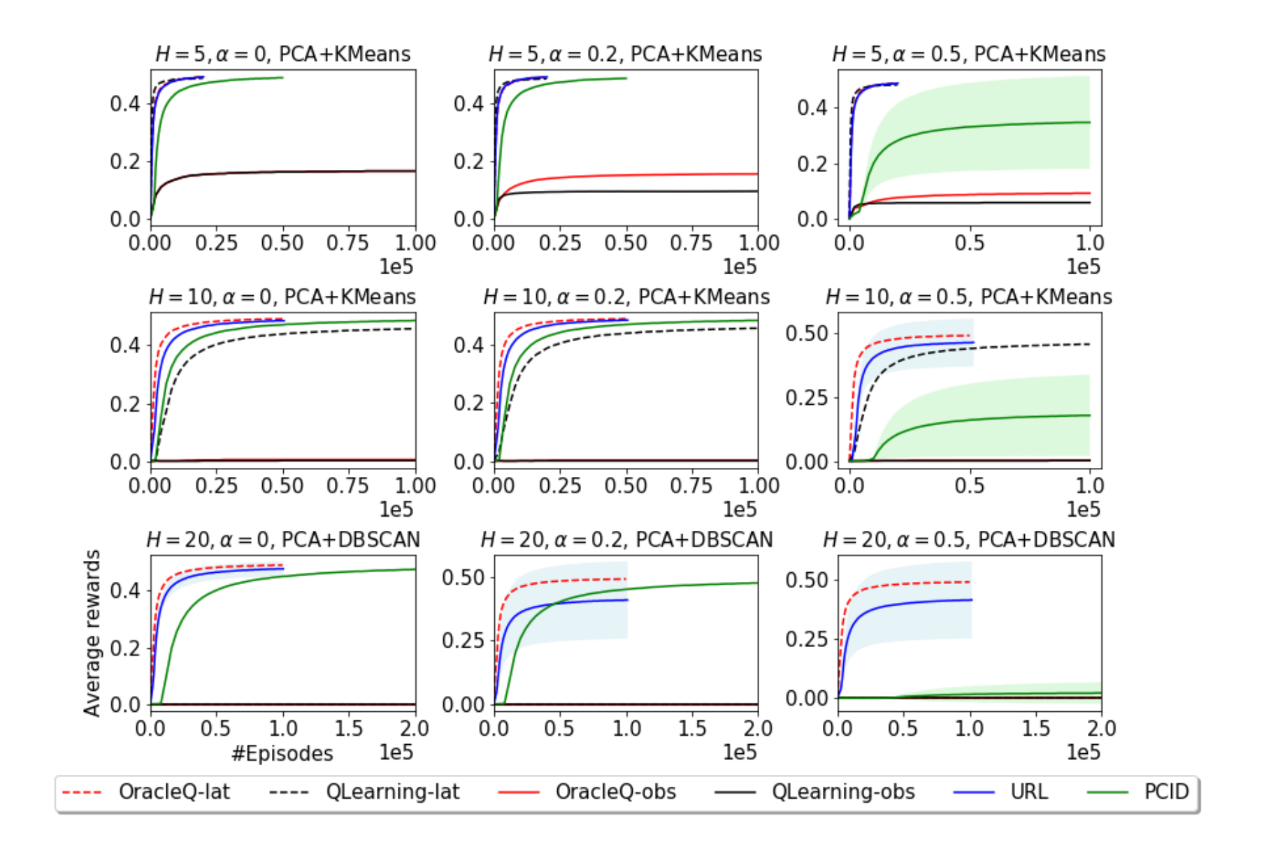
Figure 1: Performances for LockBernoulli. All lines are mean values of $50$ tests and the shaded areas depict the one standard deviations.

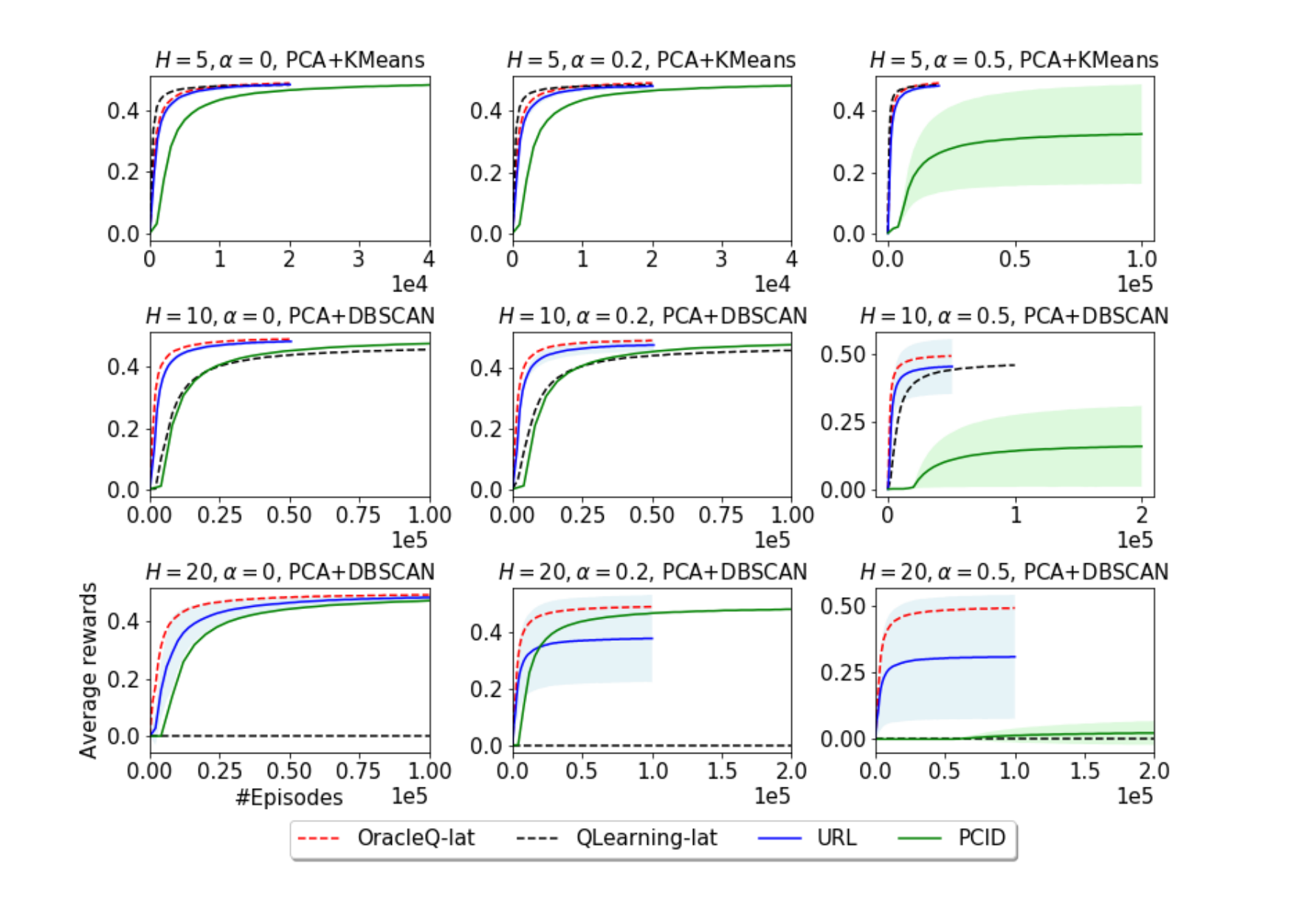
Figure 2: Performances for LockGaussian, $\sigma=0.1$. All lines are mean values of $50$ tests and the shaded areas depict the one standard deviations. OracleQ-lat and QLearning-lat have direct access to the latent states, which are not for practical use. URL and PCID only have access to the observations. OracleQ-obs and QLearning-obs are omitted due to infinitely many observations.

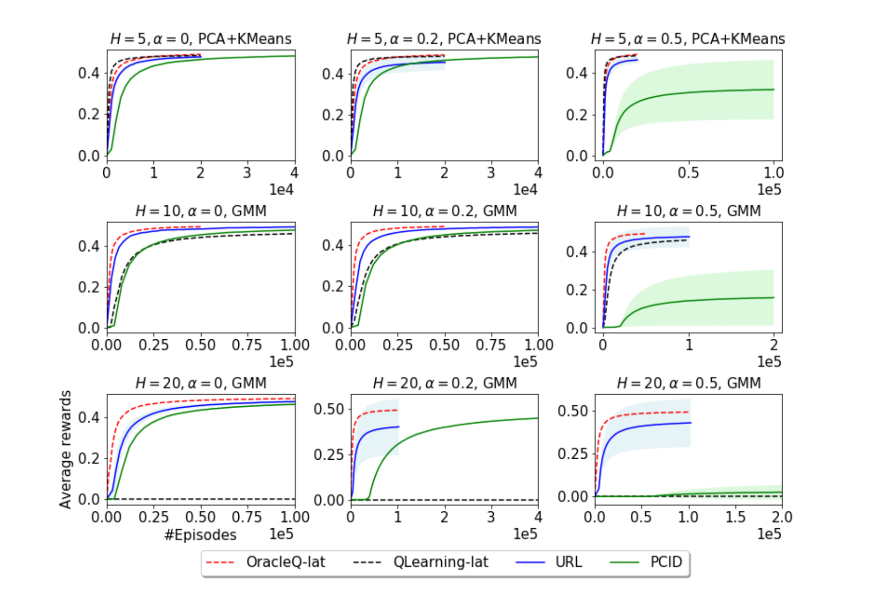
Figure 3: Performances for LockGaussian, $\sigma=0.2$. All lines are mean values of $50$ tests and the shaded areas depict the one standard deviations. OracleQ-lat and QLearning-lat have direct access to the latent states, which are not for practical use. URL and PCID only have access to the observations. OracleQ-obs and QLearning-obs are omitted due to infinitely many observations.

In this section we conduct experiments to demonstrate the effectiveness of our framework. Our code is available at https://github.com/FlorenceFeng/StateDecoding.

Environments

We conduct experiments in two environments: LockBernoulli and LockGaussian. These environments are also studied in Du et al., 2019a , which are designed to be hard for exploration. Both environments have the same latent state structure with $H$ levels, 3 states per level and 4 actions. At level $h$, from states $s_{1,h}$ and $s_{2,h}$ one action leads with probability $1-\alpha$ to $s_{1,h+1}$ and with probability $\alpha$ to $s_{2,h+1}$, another has the flipped behavior, and the remaining two lead to $s_{3,h+1}$. All actions from $s_{3,h}$ lead to $s_{3,h+1}$. Non-zero reward is only achievable if the agent can reach $s_{1,H+1}$ or $s_{2,H+1}$ and the reward follows Bernoulli(0.5). Action labels are randomly assigned at the beginning of each time of training. We consider three values of $\alpha$: 0, 0.2, and 0.5.

In LockBernoulli, the observation space is $\{0,1\}^{H+3}$ where the first 3 coordinates are reserved for the one-hot encoding of the latent state and the last $H$ coordinates are drawn i.i.d from Bernoulli(0.5). LockBernoulli meets our requirements as a BMDP. In LockGaussian, the observation space is $\mathbb{R}^{H+3}$. Every observation is constructed by first letting the first three coordinates be the one-hot encoding of the latent state, then adding i.i.d Gaussian noises ${\mathcal{N}}(0,\sigma^{2})$ to all $H+3$ coordinates. We consider $\sigma=0.1$ and $0.2$. LockGaussian is not a BMDP. We use this environment to evaluate the robustness of our method to violated assumptions.

The environments are designed to be hard for exploration. There are in total $4^{H}$ choices of actions of one episode, but only $2^{H}$ of them lead to non-zero reward in the end. So random exploration requires exponentially many trajectories. Also, with a larger $H$, the difficulty of learning accurate decoding functions increases and makes exploration with observations a more challenging task.

Algorithms and Hyperparameters

We compare 4 algorithms: OracleQ (Jin et al.,, 2019); QLearning, the tabular Q-Learning with $\epsilon$-greedy exploration; URL, our method; and PCID (Du et al., 2019a, ). For OracleQ and QLearning, there are two implementations: 1. they directly see the latent states (OracleQ-lat and QLearning-lat); 2. only see observations (OracleQ-obs and QLearning-obs). For URL and PCID, only observations are available. OracleQ-lat and QLearning-lat are served as a near-optimal skyline and a sanity-check baseline to measure the efficiency of observation-only algorithms. OracleQ-obs and QLearning-obs are only tested in LockBernoulli since there are infinitely many observations in LockGaussian. For URL, we use OracleQ as the tabular RL algorithm. Details about hyperparameters and unsupervised learning oracles in URL can be found in Appendix C.

Results

The results are presented in Figure 1, 2, and 3. $x$-axis is the number of training trajectories and $y$-axis is average reward. All lines are mean values of $50$ tests and the shaded areas depict the one standard deviations. The title for each subfigure records problem parameters and the unsupervised learning method we apply for URL. In LockBernoulli, OracleQ-obs and QLearning-obs are far from being optimal even for small-horizon cases. URL is mostly as good as the skyline (OracleQ-lat) and much better than the baseline (QLearning-lat) especially when $H=20$. URL outperforms PCID in most cases. When $H=20$, we observe a probability of $80\%$ that URL returns near-optimal values for $\alpha=0.2$ and $0.5$. In LockGaussian, for $H=20$, we observe a probability of $>75\%$ that URL returns a near-optimal policy for $\alpha=0.2$ and 0.5.

6 Conclusion

The current paper gave a general framework that turns an unsupervised learning algorithm and a no-regret tabular RL algorithm into an algorithm for RL problems with huge observation spaces. We provided theoretical analysis to show it is provably efficient. We also conducted numerical experiments to show the effectiveness of our framework in practice. An interesting future theoretical direction is to characterize the optimal sample complexity under our assumptions.

Broader Impact

Our research broadens our understanding on the use of unsupervised learning for RL, which in turn can help researchers design new principled algorithms and incorporate safety considerations for more complicated problems.

We do not believe that the results in this work will cause any ethical issue, or put anyone at a disadvantage in the society.

Acknowledgments and Disclosure of Funding

Fei Feng was supported by AFOSR MURI FA9550-18-10502 and ONR N0001417121. This work was done while Simon S. Du was at the Institute for Advanced Study and he was supported by NSF grant DMS-1638352 and the Infosys Membership.

Appendix A Proofs for the Main Result

We first give a sketch of the proof. Note that if TSR always correctly simulates a trajectory of $\pi^{k}$ on the underlying MDP, then by the correctness of ${\mathscr{A}}$, the output policy of ${\mathscr{A}}$ in the end is near-optimal with high probability. If in TSR, $f^{k,J}_{[H+1]}$ decodes states correctly (up to a fixed permutation, with high probability) for every observation generated by playing $\pi^{k}\circ f^{k,J}_{[H+1]}$, then the obtained trajectory (on ${\mathcal{S}}$) is as if obtained with $\pi^{k}\circ f_{[H+1]}$ which is essentially equal to playing $\pi^{k}$ on the underlying MDP. Let us now consider $\pi^{k}\circ f^{k,i}_{[H+1]}$ for some intermediate iteration $i\in[J]$. If there are many observations from a previously unseen state, $s$, then ${\mathcal{U}}{\mathcal{L}}{\mathcal{O}}$ guarantees that all the decoding functions in future iterations will be correct with high probability of identifying observations of $s$. Since there are at most $|{\mathcal{S}}|$ states to reach for each level following $\pi^{k}$, after $(H+1)|{\mathcal{S}}|$ iterations, TSR  is guaranteed to output a set of decoding functions that are with high probability correct under policy $\pi^{k}$. With this set of decoding functions, we can simulate a trajectory for ${\mathscr{A}}$ as if we know the true latent states.

For episode $k$, we denote the training dataset ${\mathcal{D}}$ generated by running ${\mathrm{Unif}}(\Pi)$ as $\{{\mathcal{D}}_{k,i,h}\}_{h=1}^{H+1}$ (Line 5) and the testing dataset ${\mathcal{D}}^{\prime\prime}$ generated by $\pi^{k}\circ f^{k,i-1}_{[H+1]}$ as $\{{\mathcal{D}}^{\prime\prime}_{k,i,h}\}_{h=1}^{H+1}$ (Line 6). The subscript $h$ represents the level of the observations. Furthermore, we denote by $\mu_{k,i,h}(\cdot)$ the distribution over hidden states at level $h$ induced by $\pi^{k}\circ f^{k,i-1}_{[H+1]}$. To formally prove the correctness of our framework, we first present the following lemma, showing that whenever some policy $\pi$ with some decoding functions visits a state $s$ with relatively high probability, all the decoding functions of later iterations will correctly decode the observations from $s$ with high probability.

Lemma 1.

Suppose for some $s^{*}\in{\mathcal{S}}_{h}$, $(k,i)$ is the earliest pair such that $\big{|}\{x\in{\mathcal{D}}^{\prime\prime}_{k,i,h}:f_{h}^{k,i}(x)=\alpha_{h}(s^{*})\}|\geq 3\epsilon\cdot B\log({\delta_{1}^{-1}})$ and $\{x\in{\mathcal{D}}^{\prime\prime}_{k,i,h}:f_{h}^{k,i}(x)=\alpha_{h}(s^{*})\}$ is added into ${\mathcal{Z}}_{h}$ as ${\mathcal{D}}_{h,\alpha_{h}(s^{*})}$ at line 11 Algorithm 2, where $\alpha_{h}$ is a good permutation between $f^{k,i}_{h}$ and $f_{h}$. Then for each $(k^{\prime},i^{\prime})>(k,i)$ (in lexical order), with probability at least $1-{\mathcal{O}}(\delta_{1})$,

$$\Pr_{x\sim q(\cdot|s^{*})}\big{[}f^{k^{\prime},i^{\prime}}_{h}(x)\neq\alpha_{h}^{*}(s^{*})\big{]}\leq\epsilon$$

provided $0<\epsilon\log(\delta_{1}^{-1})\leq 0.1$ and $B\geq B_{0}$. Here $B_{0}$ is some constant to be determined later and $\alpha_{h}^{*}$ is some fixed permutation on ${\mathcal{S}}_{h}$.

Proof of Lemma 1.

For iterations $(k^{\prime},i^{\prime})\geq(k,i)$, the function $\tilde{f}_{h}^{k^{\prime},i^{\prime}}$ is obtained by applying ${\mathcal{U}}{\mathcal{L}}{\mathcal{O}}$ on the dataset generated by

$$\mu^{\prime}:={\mathrm{Unif}}(\{\mu_{k^{\prime\prime},i^{\prime\prime},h}\}_{(k^{\prime\prime},i^{\prime\prime})<(k^{\prime},i^{\prime})})$$

and the dataset has size $\big{(}(k^{\prime}-1)\cdot J+i^{\prime}\big{)}\cdot B=\Theta(k^{\prime}JB)$. Thus, with probability at least $1-\delta_{1}$, for some permutation $\alpha_{h}^{\prime}$,

$$\Pr_{s\sim\mu^{\prime},x\sim q(\cdot|s)} \big{[}\tilde{f}_{h}^{k^{\prime},i^{\prime}}(x)\neq\alpha_{h}^{\prime}\circ f_{h}(x)\big{]}\leq g\big{(}\Theta(k^{\prime}JB),\delta_{1}\big{)}.$$ (1)

By taking

$$B_{0}: =\Theta\Big{(}\frac{g^{-1}(\epsilon^{2}/(K\cdot J),\delta_{1})}{K\cdot J}\Big{)},$$ (2)

we have when $B\geq B_{0}$, $g\big{(}\Theta(k^{\prime}JB),\delta_{1})\leq\epsilon^{2}/(K\cdot J)$ for all $k^{\prime}\in[K]$. Later, in Proposition 1, we will show that $B_{0}={\mathrm{poly}}(|{\mathcal{S}}|,|{\mathcal{A}}|,H,1/\varepsilon)$. Now we consider ${f}_{h}^{k,i}$. Since the FixLabel routine (Algorithm 3) does not change the accuracy ratio, from Equation (1), it holds with probability at least $1-\delta_{1}$ that

$$\Pr_{s\sim\mu_{k,i,h},x\sim q(\cdot|s)}[f^{k,i}_{h}(x)\neq\alpha_{h}\circ f_{h}(x)]\leq k\cdot J\cdot g\big{(}\Theta(kJB),\delta_{1}\big{)}\leq\epsilon.$$ (3)

Therefore, by Chernoff bound, with probability at least $1-{\mathcal{O}}(\delta_{1})$,

$$\big{|}\{x\in{\mathcal{D}}^{\prime\prime}_{k,i,h}:f_{h}(x)\neq s \text{ and }{f}_{h}^{k,i}(x)=\alpha_{h}(s)\}\big{|}<~{}\epsilon\cdot B\log({\delta_{1}^{-1}}).$$ (4)

Since $\big{|}\{x\in{\mathcal{D}}^{\prime\prime}_{k,i,h}:f_{h}^{k,i}(x)=\alpha_{h}(s^{*})\}|\geq 3\epsilon\cdot B\log({\delta_{1}^{-1}})$, we have that

$$\big{|}\{x\in{\mathcal{D}}^{\prime\prime}_{k,i,h}:~{}f_{h}(x)=s^{*}\text{ and }{f}_{h}^{k,i}(x)=\alpha_{h}(s^{*})\}|> ~{}\frac{2}{3}\cdot\big{|}\{x\in{\mathcal{D}}^{\prime\prime}_{k,i,h}:f_{h}^{k,i}(x)=\alpha_{h}(s^{*})\}\big{|}$$ (5)

$$\geq ~{}2\epsilon\cdot B\log(\delta_{1}^{-1}).$$ (6)

Thus, by Chernoff bound, with probability at least $1-{\mathcal{O}}(\delta_{1})$, $\mu_{k,i,h}(s^{*})\geq\epsilon\cdot\log(\delta_{1}^{-1}).$ Also note that $f^{k,i}_{h}$ is the first function that has confirmed on $s^{*}$ (i.e., no ${\mathcal{D}}_{h,\alpha_{h}(s^{*})}$ exists in ${\mathcal{Z}}_{h}$ of line 8 at iteration $(k,i)$). By Line 10 and Line 11, for later iterations, in ${\mathcal{Z}}_{h}$, ${\mathcal{D}}_{h,\alpha_{h}(s^{*})}=\{x\in{\mathcal{D}}^{\prime\prime}_{k,i,h}:f^{k,i}_{h}(x)=\alpha_{h}(s^{*})\}$.

Next, for another $(k^{\prime},i^{\prime})>(k,i)$, we let the corresponding permutation be $\alpha_{h}^{\prime}$ for $\tilde{f}_{h}^{k^{\prime},i^{\prime}}$. Since $\mu^{\prime}(s^{\prime})\geq\mu_{k,i,h}(s^{\prime})/(k^{\prime}\cdot J)$, with probability at least $1-\delta_{1}$,

$$\Pr_{s\sim\mu_{k,i,h},x\sim q(\cdot|s)}\big{[}\tilde{f}_{h}^{k^{\prime},i^{\prime}}(x)\neq\alpha_{h}^{\prime}\circ f_{h}(x)\big{]}\leq~{}k^{\prime}\cdot J\cdot g(\Theta(k^{\prime}JB),\delta_{1}).$$ (7)

Notice that

$$\Pr_{s\sim\mu_{k,i,h},x\sim q(\cdot|s)}\big{[}\tilde{f}_{h}^{k^{\prime},i^{\prime}}(x)\neq\alpha_{h}^{\prime}\circ f_{h}(x)\big{]}= \sum_{s^{\prime}\in{\mathcal{S}}_{h}}\mu_{k,i,h}(s^{\prime})\Pr_{x\sim q(\cdot|s^{\prime})}\big{[}\tilde{f}_{h}^{k^{\prime},i^{\prime}}(x)\neq\alpha_{h}^{\prime}\circ f_{h}(x)\big{]}$$

$$\geq ~{}\mu_{k,i,h}(s^{*})\Pr_{x\sim q(\cdot|s^{*})}\big{[}\tilde{f}_{h}^{k^{\prime},i^{\prime}}(x)\neq\alpha_{h}^{\prime}\circ f_{h}(x)\big{]}$$

$$\geq ~{}\epsilon\cdot\log(\delta^{-1})\Pr_{x\sim q(\cdot|s^{*})}\big{[}\tilde{f}_{h}^{k^{\prime},i^{\prime}}(x)\neq\alpha_{h}^{\prime}\circ f_{h}(x)\big{]}.$$

Thus, with probability at least $1-\delta_{1}$,

$$\Pr_{x\sim q(\cdot|s^{*})} \big{[}\tilde{f}_{h}^{k^{\prime},i^{\prime}}(x)\neq\alpha_{h}^{\prime}\circ f_{h}(x)\big{]}\leq\frac{k^{\prime}\cdot J\cdot g(\Theta(k^{\prime}JB),\delta_{1})}{\epsilon\cdot\log(\delta_{1}^{-1})}\leq\epsilon$$ (8)

with $B\geq B_{0}$ and $B_{0}$ as defined in Equation (2). Let $s^{\prime}:=\alpha_{h}^{\prime}(s^{*})$. Conditioning on ${\mathcal{U}}{\mathcal{L}}{\mathcal{O}}$ being correct on $\tilde{f}^{k^{\prime},i^{\prime}}_{[H+1]}$ and $f^{k,i}_{[H+1]}$, by Chernoff bound and Equation (5), with probability at least $1-{\mathcal{O}}(\delta_{1})$, we have

$$\big{|}\{x\in{\mathcal{D}}_{h,\alpha_{h}(s^{*})}:\tilde{f}_{h}^{k^{\prime},i^{\prime}}(x)=s^{\prime}\}\big{|}\geq ~{}\big{|}\{x\in{\mathcal{D}}_{h,\alpha_{h}(s^{*})}:f_{h}(x)=s^{*},\tilde{f}_{h}^{k^{\prime},i^{\prime}}(x)=s^{\prime}\}\big{|}$$

$$\geq ~{}(1-\epsilon\cdot\log(\delta_{1}^{-1}))\cdot\frac{2}{3}\cdot\big{|}{\mathcal{D}}_{h,\alpha_{h}(s^{*})}\big{|}>\frac{3}{5}\big{|}{\mathcal{D}}_{h,\alpha_{h}(s^{*})}\big{|},$$

where the fraction $\frac{2}{3}$ follows from Equation (5) and we use the fact that ${\mathcal{D}}^{\prime\prime}_{k,i,h}$ are independent from the training dataset. By our label fixing procedure, we find a permutation that swaps $s^{\prime}$ with $s$ for $\tilde{f}_{h}^{k^{\prime},i^{\prime}}$ to obtain ${f}_{h}^{k^{\prime},i^{\prime}}$. By the above analysis, with probability at least $1-{\mathcal{O}}(\delta_{1})$, $\Pr_{x\sim q(\cdot|s^{*})}\big{[}f^{k^{\prime},i^{\prime}}_{h}(x)\neq\alpha_{h}(s^{*})\big{]}\leq\epsilon$ as desired. Consequently, we let $\alpha_{h}^{*}(s^{*})=\alpha_{h}(s^{*})$, which satisfies the requirement of the lemma. ∎

Next, by the definition of our procedure of updating the label standard dataset (Line 11, Algorithm 2), we have the following corollary.

Corollary 1.

Consider Algorithm 2. Let ${\mathcal{Z}}_{k,i,h}$ be the label standard dataset at episode $k$ before iteration $i$ for ${\mathcal{S}}_{h}$. Then, with probability at least $1-{\mathcal{O}}(H|{\mathcal{S}}|\delta_{1})$,

$$\text{for all }k,i\text{ and }{\mathcal{D}}_{h,s}\in{\mathcal{Z}}_{k,i,h},|\{x\in{\mathcal{D}}_{h,s}:\alpha_{h}^{*}\circ f_{h}(x)=s,s\in{\mathcal{S}}_{h}\}|>2/3|{\mathcal{D}}_{h,s}|.$$ (9)

At episode $k$ and iteration $i$ of the algorithm TSR, let ${\mathcal{E}}_{k,i}$ be the event that for all $h\in[H+1],{\mathcal{D}}_{h,s}\in{\mathcal{Z}}_{k,i,h}$, $\Pr_{x\sim q(\cdot|s)}\big{[}f^{k,i}_{h}(x)\neq\alpha_{h}^{*}\circ f_{h}(x)\big{]}\leq\epsilon$. We have the following corollary as a consequence of Lemma 1 by taking the union bound over all states.

Corollary 2.

$\forall k,i:\quad\Pr\big{[}{\mathcal{E}}_{k,i}\big{]}\geq 1-{\mathcal{O}}(H|{\mathcal{S}}|\delta_{1}).$

The next lemma shows that after $(H+1)|{\mathcal{S}}|+1$ iterations of the TSR subroutine, the algorithm outputs a trajectory for the algorithm ${\mathscr{A}}$ as if it knows the true mapping $f_{[H+1]}$.

Lemma 2.

Suppose in an episode $k$, we are running algorithm TSR. Then after $J=(H+1)|{\mathcal{S}}|+1$ iterations, we have, for every $j\geq J$, with probability at least $1-{\mathcal{O}}(H|{\mathcal{S}}|\delta_{1})$,

$$\text{for all }h\in[H+1],\Pr_{s\sim\mu_{k,j+1,h},x\sim q(\cdot|s)}\big{[}f_{h}^{k,j}(x)\neq\alpha_{h}^{*}\circ f_{h}(x)\big{]}\leq\epsilon^{\prime}$$ (10)

for some small enough $\epsilon$ and $50H\cdot\epsilon\cdot|{\mathcal{S}}|\cdot\log(\delta_{1}^{-1})<\epsilon^{\prime}<1/2$, provided $B\geq B_{0}$ as defined in Lemma 1.

Proof of Lemma 2.

For $i<J$, there are two cases:

1. there exists an $h\in[H+1]$ such that $\Pr_{s\sim\mu_{k,i+1,h},x\sim q(\cdot|s)}\big{[}f_{h}^{k,i}(x)\neq\alpha_{h}\circ f_{h}(x)\big{]}>\epsilon^{\prime}/(2H)$;

2. for all $h\in[H+1]$, $\Pr_{s\sim\mu_{k,i+1,h},x\sim q(\cdot|s)}\big{[}f_{h}^{k,i}(x)\neq\alpha_{h}\circ f_{h}(x)\big{]}\leq\epsilon^{\prime}/(2H)$,

where $\alpha_{h}$ is some good permutations between $f^{k,i}_{h}$ and $f_{h}$. If case 1 happens, then there exists a state $s^{*}\in{\mathcal{S}}_{h}$ such that

$$\Pr_{x\sim q(\cdot|{s^{*}})}\big{[}f_{h}^{k,i}(x)\neq\alpha_{h}\circ f_{h}(x)\big{]}\cdot\mu_{k,i+1,h}(s^{*})>\frac{\epsilon^{\prime}}{2H|{\mathcal{S}}|}.$$ (11)

If ${\mathcal{D}}_{h,\alpha_{h}(s^{*})}\in{\mathcal{Z}}_{k,i,h}$, where ${\mathcal{Z}}_{k,i,h}$ is defined as in Corollary 1, by Lemma 1, with probability at least $1-{\mathcal{O}}(\delta_{1})$,

$$\Pr_{x\sim q(\cdot|s^{*})}[f_{h}^{k,i}(x)\neq\alpha_{h}^{*}\circ f_{h}(x)]\leq\epsilon$$

and $\alpha_{h}^{*}(s^{*})=\alpha_{h}(s^{*})$. Thus, $\mu_{k,i+1,h}(s^{*})>\frac{\epsilon^{\prime}}{2H|{\mathcal{S}}|}/\epsilon>1$, a contradiction with $\mu_{k,i+1,h}(s^{*})\leq 1$. Therefore, there is no ${\mathcal{D}}_{h,\alpha_{h}(s^{*})}$ in ${\mathcal{Z}}_{k,i,h}$. Then, due to $\Pr_{x\sim q(\cdot|s^{*})}\big{[}f_{h}^{k,i}(x)\neq\alpha_{h}\circ f_{h}(x)\big{]}\leq 1$, by Equation (11), we have

$$\mu_{k,i+1,h}(s^{*})>\frac{\epsilon^{\prime}}{2H|{\mathcal{S}}|}.$$ (12)

Since $f^{k,i+1}_{h}$ is trained on ${\mathrm{Unif}}(\{\mu_{k^{\prime},i^{\prime},h}\}_{(k^{\prime},i^{\prime})<(k,i+1)})$, by Definition of ${\mathcal{U}}{\mathcal{L}}{\mathcal{O}}$, with probability at least $1-\delta_{1}$,

$$\Pr_{s\sim\mu_{k,i+1,h},x\sim q(\cdot|s)}\big{[}f^{k,i+1}_{h}(x)\neq\alpha_{h}^{\prime}(s)\big{]}\leq k\cdot J\cdot g(\Theta(kJB),\delta_{1})\leq\epsilon^{2},$$ (13)

with $B\geq B_{0}$ ($B_{0}$ is defined in Equation (2)) and $\alpha_{h}^{\prime}$ is some good permutation between $f^{k,i+1}_{h}$ and $f_{h}$. Thus, by Equation (12) and the choice of $\epsilon$ and $\epsilon^{\prime}$, we have

$$\Pr_{x\sim q(\cdot|s^{*})}\big{[}f^{k,i+1}_{h}(x)\neq\alpha_{h}^{\prime}(s^{*})\big{]}<\epsilon/25.$$ (14)

Thus,

$$\mu_{k,i+1,h}(s^{*})\cdot\Pr_{x\sim q(\cdot|s^{*})}\big{[}f^{k,i+1}_{h}(x)=\alpha_{h}^{\prime}(s^{*})\big{]}>\frac{\epsilon^{\prime}}{2H|{\mathcal{S}}|}\cdot(1-\epsilon/25)>24\epsilon\cdot\log(\delta_{1}^{-1}),$$ (15)

where the last inequality is due to $\epsilon<\epsilon^{\prime}<1$. By Chernoff bound, with probability at least $1-{\mathcal{O}}(\delta_{1})$,

$$|\{x\in{\mathcal{D}}^{\prime\prime}_{k,i+1,h}:f^{k,i+1}_{h}(x)=\alpha_{h}^{\prime}(s^{*})\}|\geq 3\epsilon\cdot B\log(\delta_{1}^{-1}).$$

Therefore, if case 1 happens, one state $s$ will be confirmed in iteration $i+1$ and $\alpha_{h}^{*}(s^{*})=\alpha_{h}^{\prime}(s^{*})$ is defined.

To analyze case 2, we first define sets $\{{\mathcal{G}}_{k,i+1,h}\}_{h=1}^{H+1}$ with ${\mathcal{G}}_{k,i+1,h}:=\{s\in{\mathcal{S}}_{h}~{}|~{}{\mathcal{D}}_{h,s}\in{\mathcal{Z}}_{k,i+1,h}\}$, i.e., ${\mathcal{G}}_{k,i+1,h}$ contains all confirmed states of level $h$ before iteration $i+1$ at episode $k$. If case 2 happens, we further divide the situation into two subcases:

1. for all $h\in[H+1]$, for all $s\in{\mathcal{G}}^{c}_{k,i+1,h}$, $\mu_{k,i+1,h}(s)\leq\epsilon^{\prime}/(8H|{\mathcal{S}}|)$;

2. there exists an $h\in[H+1]$ and a state $s^{*}\in{\mathcal{G}}^{c}_{k,i+1,h}$ such that $\mu_{k,i+1,h}(s^{*})\geq\epsilon^{\prime}/(8H|{\mathcal{S}}|)$,

First notice that for every $h\in[H+1]$ and $j>i$, since $f^{k,j}_{h}$ is trained on ${\mathrm{Unif}}(\{\mu_{k^{\prime},i^{\prime},h}\}_{(k^{\prime},i^{\prime})\leq(k,j)})$, by Definition of ${\mathcal{U}}{\mathcal{L}}{\mathcal{O}}$ and our choice of $B$ in Equation (2), with probability at least $1-\delta_{1}$, we have

$$\Pr_{s\sim\mu_{k,i+1,h},x\sim q(\cdot|s)}[f^{k,j}_{h}\neq\alpha_{h}^{\prime}(s)]\leq\epsilon^{2},$$ (16)

$$\Rightarrow \sum_{s\in{\mathcal{G}}_{k,i+1,h}}\mu_{k,i+1,h}(s)\Pr_{x\sim q(\cdot|s)}[f^{k,j}_{h}(x)\neq\alpha_{h}^{\prime}(s)]+\sum_{s\notin{\mathcal{G}}_{k,i+1,h}}\mu_{k,i+1,h}(s)\Pr_{x\sim q(\cdot|s)}[f^{k,j}_{h}(x)\neq\alpha_{h}^{\prime}(s)]\leq\epsilon^{2},$$ (17)

where $\alpha_{h}^{\prime}$ is some good permutation between $f^{k,j}_{h}$ and $f_{h}$.

If subcase a) happens, note that for $s\in{\mathcal{G}}_{k,i+1,h}$, due to the FixLabel routine (Algorithm 3), $\alpha_{h}^{\prime}(s)=\alpha_{h}^{*}(s)$, for $f^{k,j}_{h}(j>i)$ we have

$$\sum_{s\in{\mathcal{S}}_{h}}\mu_{k,i+1,h}(s)\Pr_{x\sim q(\cdot|s)}[f^{k,j}_{h}(x)\neq\alpha_{h}^{*}(s)]$$ (18)

$$= \sum_{s\in{\mathcal{G}}_{k,i+1,h}}\mu_{k,i+1,h}(s)\Pr_{x\sim q(\cdot|s)}[f^{k,j}_{h}(x)\neq\alpha_{h}^{*}(s)]+\sum_{s\notin{\mathcal{G}}_{k,i+1,h}}\mu_{k,i+1,h}(s)\Pr_{x\sim q(\cdot|s)}[f^{k,j}_{h}(x)\neq\alpha_{h}^{*}(s)]$$ (19)

$$= \sum_{s\in{\mathcal{G}}_{k,i+1,h}}\mu_{k,i+1,h}(s)\Pr_{x\sim q(\cdot|s)}[f^{k,j}_{h}(x)\neq\alpha_{h}^{\prime}(s)]+\sum_{s\notin{\mathcal{G}}_{k,i+1,h}}\mu_{k,i+1,h}(s)\Pr_{x\sim q(\cdot|s)}[f^{k,j}_{h}(x)\neq\alpha_{h}^{*}(s)]$$ (20)

$$\leq ~{}\epsilon^{2}+\epsilon^{\prime}/(8H)<\epsilon^{\prime}/(4H).$$ (21)

Taking a union bound over all $f^{k,j}_{[H+1]}$, we have that for any $h\in[H+1]$, with probability at least $1-{\mathcal{O}}(H\delta_{1})$,

$$\Pr_{s\sim\mu_{k,j+1,h},x\sim q(\cdot|s)}[f^{k,j}_{h}(x)=\alpha_{h}^{*}(s)]\geq\Pr_{s\sim\mu_{k,j+1,h},x\sim q(\cdot|s)}[f^{k,j}_{h}(x)=\alpha_{h}^{*}(s)=f^{k,i}_{h}(x)]$$ (22)

$$\geq\Pr_{\text{for all~{}}h^{\prime}\in[h],s_{h^{\prime}}\sim\mu_{k,j+1,h^{\prime}},x_{h^{\prime}}\sim q(\cdot|s_{h^{\prime}})}[\text{ for all }h^{\prime}\in[h],f^{k,j}_{h^{\prime}}(x_{h^{\prime}})=\alpha_{h^{\prime}}^{*}(s)=f^{k,i}_{h^{\prime}}(x_{h^{\prime}})]$$ (23)

$$=\Pr_{\text{for all~{}}h^{\prime}\in[h],s_{h^{\prime}}\sim\mu_{k,i+1,h^{\prime}},x_{h^{\prime}}\sim q(\cdot|s_{h^{\prime}})}[\text{ for all }h^{\prime}\in[h],f^{k,j}_{h^{\prime}}(x_{h^{\prime}})=\alpha_{h^{\prime}}^{*}(s)=f^{k,i}_{h^{\prime}}(x_{h^{\prime}})]$$ (24)

$$\geq 1-(\epsilon^{\prime}/(2H)+\epsilon^{\prime}/(4H))\cdot H\geq 1-\epsilon^{\prime}.$$ (25)

Therefore, if case 2 and subcase a) happens, the desired result is obtained.

If subcase b) happens, we consider the function $f^{k,i+1}_{h}$. By Equation (16),

$$\mu_{k,i+1,h}(s^{*})\cdot\Pr_{x\sim q(\cdot|s^{*})}[f^{k,i+1}_{h}(x)\neq\alpha_{h}^{\prime}(s^{*})]\leq\epsilon^{2}$$ (26)

$$\Rightarrow \Pr_{x\sim q(\cdot|s^{*})}[f^{k,i+1}_{h}(x)\neq\alpha_{h}^{\prime}(s^{*})]\leq\epsilon^{2}/(\epsilon^{\prime}/(8H|{\mathcal{S}}|))\leq\epsilon,$$ (27)

where $\alpha_{h}^{\prime}$ here is some good permutation between $f^{k,i+1}_{h}$ and $f_{h}$. Thus,

$$\mu_{k,i+1,h}(s^{*})\cdot\Pr_{x\sim q(\cdot|s^{*})}\big{[}f^{k,i+1}_{h}(x)=\alpha_{h}^{\prime}(s^{*})\big{]}>\frac{\epsilon^{\prime}}{8H|{\mathcal{S}}|}\cdot(1-\epsilon)>6\epsilon\cdot\log(\delta_{1}^{-1}).$$ (28)

By Chernoff bound, with probability at least $1-{\mathcal{O}}(\delta_{1})$, $|\{x\in{\mathcal{D}}^{\prime\prime}_{k,i+1,h}:f^{k,i+1}_{h}(x)=\alpha_{h}^{\prime}(s^{*})\}|\geq 3\epsilon\cdot B\log(\delta_{1}^{-1}).$ Therefore, the state $s^{*}$ will be confirmed in iteration $i+1$ and $\alpha_{h}^{*}(s^{*})=\alpha_{h}^{\prime}(s^{*})$ is defined.

In conclusion, for each iteration, there are two scenarios, either the desired result in Lemma 2 holds already or a new state will be confirmed for the next iteration. Since there are in total $\sum_{h=1}^{H+1}|{\mathcal{S}}_{h}|\leq(H+1)|{\mathcal{S}}|$ states, after $J:=(H+1)|{\mathcal{S}}|+1$ iterations, by Lemma 1, with probability at least $1-{\mathcal{O}}(H|{\mathcal{S}}|\delta_{1})$, for every $j\geq J$, for all $h\in[H+1]$ and all $s\in{\mathcal{S}}_{h}$, we have $\Pr_{x\sim q(\cdot|s)}[f^{k,j}_{h}(x)\neq\alpha_{h}^{*}(s)]\leq\epsilon$. Therefore, it holds that for

$$\Pr_{s\sim\mu_{k,j+1,h},x\sim q(\cdot|s)}(f^{k,j}_{h}(x)\neq\alpha_{h}^{*}(s))\leq\epsilon<\epsilon^{\prime}.$$ (29)

∎

Proposition 1.

Suppose in Definition 1, $g^{-1}(\epsilon,\delta_{1})={\mathrm{poly}}(1/\epsilon,\log(\delta^{-1}_{1}))$ for any $\epsilon,\delta_{1}\in(0,1)$ and ${\mathscr{A}}$ is $(\varepsilon,\delta_{2})$-correct with sample complexity ${\mathrm{poly}}\left(|{\mathcal{S}}|,|{\mathcal{A}}|,H,1/\varepsilon,\log\left(\delta^{-1}_{2}\right)\right)$ for any $\varepsilon,\delta_{2}\in(0,1)$. Then for each iteration of the outer loop of Algorithm 1, the policy $\phi^{n}$ is an $\varepsilon/3$-optimal policy for the BMDP with probability at least $0.99$, using at most ${\mathrm{poly}}\left(|{\mathcal{S}}|,|{\mathcal{A}}|,H,1/\varepsilon\right)$ trajectories.

Proof of Proposition 1.

We first show that the trajectory obtained by running $\pi^{k}$ with the learned decoding functions $f^{k,J}_{[H+1]}$ matches, with high probability, that from running $\pi^{k}$ with $\alpha_{[H+1]}^{*}\circ f_{[H+1]}$. Let $K=C(\varepsilon/4,\delta_{2})$ be the total number of episodes played by ${\mathscr{A}}$ to learn an $\varepsilon/4$-optimal policy with probability at least $1-\delta_{2}$. For each episode $k\in[K]$, let the trajectory of observations be $\{x^{k}_{h}\}_{h=1}^{H+1}$. We define event

$${\mathcal{E}}_{k}:=\{\forall h\in[H+1],f^{k,J}_{h}(x^{k}_{h})=\alpha_{h}^{*}(f_{h}(x^{k}_{h}))\},$$

where $J=(H+1)|{\mathcal{S}}|+1$. Note that on ${\mathcal{E}}_{k}$, the trajectory of running $\pi^{k}\circ\alpha^{*}_{[H+1]}\circ f_{[H+1]}$ equals running $\pi^{k}\circ f^{k,J}_{[H+1]}$. We also let the event ${\mathcal{F}}$ be that ${\mathcal{U}}{\mathcal{L}}{\mathcal{O}}$ succeeds on every iteration (satisfies Lemma 2). Thus,

$$\Pr[{\mathcal{F}}]\geq 1-K\cdot J\cdot\delta_{1}=1-{\mathrm{poly}}(|{\mathcal{S}}|,|{\mathcal{A}}|,H,1/\varepsilon,\log(\delta_{1}^{-1}))\cdot\delta_{1}.$$

Furthermore, each $x_{k,h}$ is obtained by the distribution $\sum_{s}\mu_{k,J+1,h}(s)q(\cdot|s)$. On ${\mathcal{F}}$, by Lemma 2, we have

$$\Pr[f^{k,J}_{h}(x^{k}_{h})=\alpha_{h}^{*}(f_{h}(x^{k}_{h}))]\leq\epsilon^{\prime}$$

by the choice of $B$. Therefore,

$$\Pr[{\mathcal{E}}_{k}|{\mathcal{F}}]\geq 1-(H+1)\epsilon^{\prime}.$$

Overall, we have

$$\Pr\Big{[}{\mathcal{E}}_{k},~{}\forall k\in[K]\Big{|}{\mathcal{F}}\Big{]}\geq 1-K(H+1)\epsilon^{\prime}.$$

Thus, with probability at least $1-\delta_{2}-{\mathrm{poly}}(|{\mathcal{S}}|,|{\mathcal{A}}|,H,1/\varepsilon,\log(\delta_{1}^{-1}))\cdot(\epsilon^{\prime}+\delta_{1})$, ${\mathcal{A}}$ outputs a policy $\pi$, that is $\varepsilon/4$-optimal for the underlying MDP with state sets $\{{\mathcal{S}}_{h}\}_{h=1}^{H+1}$ permutated by $\alpha_{[H+1]}^{*}$, which we denote as event ${\mathcal{E}}^{\prime}$. Conditioning on ${\mathcal{E}}^{\prime}$, since on a high probability event ${\mathcal{E}}^{\prime\prime}$ with $\Pr[{\mathcal{E}}^{\prime\prime}]\geq 1-(H+1)\epsilon^{\prime}$, $\pi\circ f_{[H+1]}^{K,J}$ and $\pi\circ\alpha^{*}_{[H+1]}\circ f_{[H+1]}$ have the same trajectory, the value achieved by $\pi\circ f_{[H+1]}^{K,J}$ and $\pi\circ\alpha^{*}_{[H+1]}\circ f_{[H+1]}$ differ by at most $(H+1)^{2}\epsilon^{\prime}$. Thus, with probability at least $1-\delta_{2}-{\mathrm{poly}}(|{\mathcal{S}}|,|{\mathcal{A}}|,H,1/\varepsilon,\log(\delta_{1}^{-1}))\cdot(\epsilon^{\prime}+\delta_{1})$, the output policy $\pi\circ f_{[H+1]}^{K,J}$ is at least $\varepsilon/4+{\mathcal{O}}(H^{2}\epsilon^{\prime})$ accurate, i.e.,

$$V_{1}^{*}-V_{1}^{\pi\circ f_{[H+1]}^{K,J}}\leq ~{}V_{1}^{*}-V_{1}^{\pi\circ\alpha^{*}_{[H+1]}\circ f_{[H+1]}}+~{}{\mathcal{O}}(H^{2}\epsilon^{\prime})\leq~{}\varepsilon/4~{}+~{}{\mathcal{O}}(H^{2}\epsilon^{\prime}).$$ (30)

Setting $\epsilon^{\prime}$, $\delta_{1}$, and $\delta_{2}$ properly, $V_{1}^{*}-V_{1}^{\pi\circ f_{[H+1]}^{K,J}}\leq\varepsilon/3$ with probability at least $0.99$. Since $1/\delta_{1}={\mathrm{poly}}(|{\mathcal{S}}|,|{\mathcal{A}}|,H,1/\varepsilon)$ and $1/\epsilon={\mathrm{poly}}(|{\mathcal{S}}|,|{\mathcal{A}}|,H,1/\varepsilon,\log(\delta_{1}^{-1}))$, $B_{0}$ in Lemma 1 and Lemma 2 is ${\mathrm{poly}}(|{\mathcal{S}}|,|{\mathcal{A}}|,H,1/\varepsilon)$. The desired result is obtained. ∎

Finally, based on Proposition 1, we establish Theorem 1.

Proof of Theorem 1.

By Proposition 1 and taking $N=\lceil\log(2/\delta)/2\rceil$, with probability at least $1-\delta/2$, there exists a policy in $\{\phi^{n}\}_{n=1}^{N}$ that is $\varepsilon/3$-optimal for the BMDP. For each policy $\phi^{n}$, we take $L:=\lceil 9H^{2}/(2\varepsilon^{2})\log(2N/\delta)\rceil$ episodes to evaluate its value. Then by Hoeffding’s inequality, with probability at least $1-\delta/(2N)$, $|\bar{V}_{1}^{\phi^{n}}-V_{1}^{\phi^{n}}|\leq\varepsilon/3.$ By taking the union bound and selecting the policy $\phi\in\operatorname*{argmax}_{\phi\in\phi^{[N]}}\bar{V}_{1}^{\phi}$, with probability at least $1-\delta$, it is $\varepsilon$-optimal for the BMDP. In total, the number of needed trajectories is $N\cdot\sum_{k=1}^{K}\sum_{i=1}^{J}\big{(}(k-1)J+i+1\big{)}B+N\cdot L={\mathcal{O}}(N\cdot K^{2}\cdot J^{2}\cdot B+N\cdot L)={\mathrm{poly}}(|{\mathcal{S}}|,|{\mathcal{A}}|,H,1/\varepsilon,\log(\delta^{-1})).$ We complete the proof. ∎

Appendix B Examples of Unsupervised Learning Oracle

In this section, we give some examples of ${\mathcal{U}}{\mathcal{L}}{\mathcal{O}}$. First notice that the generation process of ${\mathcal{U}}{\mathcal{L}}{\mathcal{O}}$ is termed as the mixture model in statistics (McLachlan and Basford,, 1988; McLachlan and Peel,, 2004), which has a wide range of applications (see e.g., Bouguila and Fan, (2020)). We list examples of mixture models and some algorithms as candidates of ${\mathcal{U}}{\mathcal{L}}{\mathcal{O}}$.

Gaussian Mixture Models (GMM)

In GMM, $q(\cdot|s)={\mathcal{N}}(s,\sigma_{s}^{2})$, i.e., observations are hidden states plus Gaussian noise. When the noises are (truncated) Gaussian, under certain conditions, e.g. states are well-separated, we are able to identify the latent states with high accuracy. A series of works (Arora and Kannan,, 2001; Vempala and Wang,, 2004; Achlioptas and McSherry,, 2005; Dasgupta and Schulman,, 2000; Regev and Vijayaraghavan,, 2017) proposed algorithms that can be served as ${\mathcal{U}}{\mathcal{L}}{\mathcal{O}}$.

Bernoulli Mixture Models (BMM)

BMM is considered in binary image processing (Juan and Vidal,, 2004) and texts classification (Juan and Vidal,, 2002). In BMM, every observation is a point in $\{0,1\}^{d}$. A true state determines a frequency vector. In Najafi et al., (2020), the authors proposed a reliable clustering algorithm for BMM data with polynomial sample complexity guarantee.

Subspace Clustering

In some applications, each state is a set of vectors and observations lie in the spanned subspace. Suppose for different states, the basis vectors differ under certain metric, then recovering the latent state is equivalent to subspace clustering. Subspace clustering has a variety of applications include face clustering, community clustering, and DNA sequence analysis (Wallace et al.,, 2015; Vidal,, 2011; Elhamifar and Vidal,, 2013). Proper algorithms for ${\mathcal{U}}{\mathcal{L}}{\mathcal{O}}$ can be found in e.g., (Wang et al.,, 2013; Soltanolkotabi et al.,, 2014).

In addition to the aforementioned models, other reasonable settings are Categorical Mixture Models (Bontemps and Toussile,, 2013), Poisson Mixture Models (Li and Zha,, 2006), Dirichlet Mixture Models (Dahl,, 2006) and so on.

Appendix C More about Experiments

Parameter Tuning

In the experiments, for OracleQ, we tune the learning rate and a confidence parameter; for QLearning, we tune the learning rate and the exploration parameter $\epsilon$; for PCID, we follow the code provided in Du et al., 2019a , tune the number of clusters for $k$-means and the number of trajectories $n$ to collect in each outer iteration, and finally select the better result between linear function and neural network implementation.

Unsupervised Learning Algorithms

In our method, we use OracleQ as the tabular RL algorithm to operate on the decoded state space and try three unsupervised learning approaches: 1. first conduct principle component analysis (PCA) on the observations and then use $k$-means (KMeans) to cluster; 2. first apply PCA, then use Density-Based Spatial Clustering of Applications with Noise (DBSCAN) for clustering, and finally use support vector machine to fit a classifier; 3. employ Gaussian Mixture Model (GMM) to fit the observation data then generate a label predictor. We call the python library sklearn for all these methods. During unsupervised learning, we do not separate observations by levels but add level information in decoded states. Besides the hyperparameters for OracleQ and the unsupervised learning oracle, we also tune the batch size $B$ adaptively in Algorithm 2. In our tests, instead of resampling over all previous policies as Line 5 Algorithm 2, we use previous data. Specifically, we maintain a training dataset ${\mathcal{D}}$ in memory and for iteration $i$, generate $B$ training trajectories following $\pi\circ f^{i-1}_{[H+1]}$ and merge them into ${\mathcal{D}}$ to train ${\mathcal{U}}{\mathcal{L}}{\mathcal{O}}$. Also, we stop training decoding functions once they become stable, which takes $100$ training trajectories when $H=5$, $500\sim 1000$ trajectories when $H=10$, and $1000\sim 2500$ trajectories when $H=20$. Since this process stops very quickly, we also skip the label matching steps (Line 8 to Line 12 Algorithm 2) and the final decoding function leads to a near-optimal performance as shown in the results.

References

- Achlioptas and McSherry, (2005) Achlioptas, D. and McSherry, F. (2005). On spectral learning of mixtures of distributions. In International Conference on Computational Learning Theory, pages 458–469. Springer.
- Agarwal et al., (2019) Agarwal, A., Kakade, S. M., Lee, J. D., and Mahajan, G. (2019). Optimality and approximation with policy gradient methods in Markov decision processes. arXiv preprint arXiv:1908.00261.
- Agrawal and Jia, (2017) Agrawal, S. and Jia, R. (2017). Optimistic posterior sampling for reinforcement learning: Worst-case regret bounds. In Proceedings of the 31st International Conference on Neural Information Processing Systems, pages 1184–1194. Curran Associates Inc.
- Antos et al., (2008) Antos, A., Szepesvári, C., and Munos, R. (2008). Learning near-optimal policies with Bellman-residual minimization based fitted policy iteration and a single sample path. Machine Learning, 71(1):89–129.
- Arora and Kannan, (2001) Arora, S. and Kannan, R. (2001). Learning mixtures of arbitrary Gaussians. In Proceedings of the thirty-third annual ACM symposium on Theory of computing, pages 247–257.
- Azar et al., (2017) Azar, M. G., Osband, I., and Munos, R. (2017). Minimax regret bounds for reinforcement learning. In Proceedings of the 34th International Conference on Machine Learning-Volume 70, pages 263–272. JMLR. org.
- Azizzadenesheli et al., (2018) Azizzadenesheli, K., Brunskill, E., and Anandkumar, A. (2018). Efficient exploration through Bayesian deep Q-networks. In 2018 Information Theory and Applications Workshop (ITA), pages 1–9.
- Bagnell et al., (2004) Bagnell, J. A., Kakade, S. M., Schneider, J. G., and Ng, A. Y. (2004). Policy search by dynamic programming. In Advances in neural information processing systems, pages 831–838.
- Bellemare et al., (2016) Bellemare, M., Srinivasan, S., Ostrovski, G., Schaul, T., Saxton, D., and Munos, R. (2016). Unifying count-based exploration and intrinsic motivation. In Advances in Neural Information Processing Systems, pages 1471–1479.
- Bontemps and Toussile, (2013) Bontemps, D. and Toussile, W. (2013). Clustering and variable selection for categorical multivariate data. Electronic Journal of Statistics, 7:2344–2371.
- Bouguila and Fan, (2020) Bouguila, N. and Fan, W. (2020). Mixture models and applications. Springer.
- Charikar, (2002) Charikar, M. S. (2002). Similarity estimation techniques from rounding algorithms. In Proceedings of the thiry-fourth annual ACM symposium on Theory of computing, pages 380–388.
- Chen and Jiang, (2019) Chen, J. and Jiang, N. (2019). Information-theoretic considerations in batch reinforcement learning. In International Conference on Machine Learning, pages 1042–1051.
- Dahl, (2006) Dahl, D. B. (2006). Model-based clustering for expression data via a Dirichlet process mixture model. Bayesian inference for gene expression and proteomics, 4:201–218.
- Dann et al., (2018) Dann, C., Jiang, N., Krishnamurthy, A., Agarwal, A., Langford, J., and Schapire, R. E. (2018). On oracle-efficient PAC RL with rich observations. In Advances in Neural Information Processing Systems, pages 1422–1432.
- Dann et al., (2017) Dann, C., Lattimore, T., and Brunskill, E. (2017). Unifying PAC and regret: Uniform PAC bounds for episodic reinforcement learning. In Proceedings of the 31st International Conference on Neural Information Processing Systems, NIPS’17, pages 5717–5727, USA. Curran Associates Inc.
- Dasgupta and Schulman, (2000) Dasgupta, S. and Schulman, L. J. (2000). A two-round variant of EM for Gaussian mixtures. In Proceedings of the Sixteenth conference on Uncertainty in artificial intelligence, pages 152–159.
- (18) Du, S., Krishnamurthy, A., Jiang, N., Agarwal, A., Dudik, M., and Langford, J. (2019a). Provably efficient RL with rich observations via latent state decoding. In International Conference on Machine Learning, pages 1665–1674.
- (19) Du, S. S., Kakade, S. M., Wang, R., and Yang, L. F. (2020a). Is a good representation sufficient for sample efficient reinforcement learning? In International Conference on Learning Representations.
- (20) Du, S. S., Lee, J. D., Mahajan, G., and Wang, R. (2020b). Agnostic Q-learning with function approximation in deterministic systems: Tight bounds on approximation error and sample complexity. arXiv preprint arXiv:2002.07125.
- (21) Du, S. S., Luo, Y., Wang, R., and Zhang, H. (2019b). Provably efficient Q-learning with function approximation via distribution shift error checking oracle. In Advances in Neural Information Processing Systems, pages 8058–8068.
- Elhamifar and Vidal, (2013) Elhamifar, E. and Vidal, R. (2013). Sparse subspace clustering: Algorithm, theory, and applications. IEEE transactions on pattern analysis and machine intelligence, 35(11):2765–2781.
- Fortunato et al., (2018) Fortunato, M., Azar, M. G., Piot, B., Menick, J., Hessel, M., Osband, I., Graves, A., Mnih, V., Munos, R., Hassabis, D., Pietquin, O., Blundell, C., and Legg, S. (2018). Noisy networks for exploration. In International Conference on Learning Representations.
- Geist et al., (2019) Geist, M., Scherrer, B., and Pietquin, O. (2019). A theory of regularized Markov decision processes. In International Conference on Machine Learning, pages 2160–2169.
- Jaksch et al., (2010) Jaksch, T., Ortner, R., and Auer, P. (2010). Near-optimal regret bounds for reinforcement learning. Journal of Machine Learning Research, 11(Apr):1563–1600.
- Jiang et al., (2017) Jiang, N., Krishnamurthy, A., Agarwal, A., Langford, J., and Schapire, R. E. (2017). Contextual decision processes with low Bellman rank are PAC-learnable. In Proceedings of the 34th International Conference on Machine Learning-Volume 70, pages 1704–1713. JMLR. org.
- Jin et al., (2018) Jin, C., Allen-Zhu, Z., Bubeck, S., and Jordan, M. I. (2018). Is Q-learning provably efficient? In Advances in Neural Information Processing Systems, pages 4863–4873.
- Jin et al., (2019) Jin, C., Yang, Z., Wang, Z., and Jordan, M. I. (2019). Provably efficient reinforcement learning with linear function approximation. arXiv preprint arXiv:1907.05388.
- Juan and Vidal, (2002) Juan, A. and Vidal, E. (2002). On the use of Bernoulli mixture models for text classification. Pattern Recognition, 35(12):2705–2710.
- Juan and Vidal, (2004) Juan, A. and Vidal, E. (2004). Bernoulli mixture models for binary images. In Proceedings of the 17th International Conference on Pattern Recognition, 2004. ICPR 2004., volume 3, pages 367–370. IEEE.
- Kakade and Langford, (2002) Kakade, S. and Langford, J. (2002). Approximately optimal approximate reinforcement learning. In ICML, volume 2, pages 267–274.
- Kakade et al., (2018) Kakade, S., Wang, M., and Yang, L. F. (2018). Variance reduction methods for sublinear reinforcement learning. arXiv preprint arXiv:1802.09184.
- Kearns and Singh, (2002) Kearns, M. and Singh, S. (2002). Near-optimal reinforcement learning in polynomial time. Machine learning, 49(2-3):209–232.
- Krishnamurthy et al., (2016) Krishnamurthy, A., Agarwal, A., and Langford, J. (2016). PAC reinforcement learning with rich observations. In Advances in Neural Information Processing Systems, pages 1840–1848.
- Li and Zha, (2006) Li, J. and Zha, H. (2006). Two-way Poisson mixture models for simultaneous document classification and word clustering. Computational Statistics & Data Analysis, 50(1):163–180.
- Li et al., (2011) Li, L., Littman, M. L., Walsh, T. J., and Strehl, A. L. (2011). Knows what it knows: A framework for self-aware learning. Machine learning, 82(3):399–443.
- Lipton et al., (2018) Lipton, Z. C., Li, X., Gao, J., Li, L., Ahmed, F., and Deng, L. (2018). BBQ-networks: Efficient exploration in deep reinforcement learning for task-oriented dialogue systems. In AAAI.
- McLachlan and Basford, (1988) McLachlan, G. J. and Basford, K. E. (1988). Mixture models: Inference and applications to clustering, volume 38. M. Dekker New York.
- McLachlan and Peel, (2004) McLachlan, G. J. and Peel, D. (2004). Finite mixture models. John Wiley & Sons.
- Munos, (2005) Munos, R. (2005). Error bounds for approximate value iteration. In Proceedings of the National Conference on Artificial Intelligence, volume 20, page 1006. Menlo Park, CA; Cambridge, MA; London; AAAI Press; MIT Press; 1999.
- Najafi et al., (2020) Najafi, A., Motahari, S. A., and Rabiee, H. R. (2020). Reliable clustering of Bernoulli mixture models. Bernoulli, 26(2):1535–1559.
- Ni et al., (2019) Ni, C., Yang, L. F., and Wang, M. (2019). Learning to control in metric space with optimal regret. In 2019 57th Annual Allerton Conference on Communication, Control, and Computing (Allerton), pages 726–733.
- Osband et al., (2016) Osband, I., Van Roy, B., and Wen, Z. (2016). Generalization and exploration via randomized value functions. In Proceedings of the 33rd International Conference on International Conference on Machine Learning - Volume 48, ICML’16, pages 2377–2386. JMLR.org.
- Pathak et al., (2017) Pathak, D., Agrawal, P., Efros, A. A., and Darrell, T. (2017). Curiosity-driven exploration by self-supervised prediction. In International Conference on Machine Learning (ICML), volume 2017.
- Pazis and Parr, (2013) Pazis, J. and Parr, R. (2013). PAC optimal exploration in continuous space Markov decision processes. In Proceedings of the Twenty-Seventh AAAI Conference on Artificial Intelligence, AAAI’13, pages 774–781. AAAI Press.
- Regev and Vijayaraghavan, (2017) Regev, O. and Vijayaraghavan, A. (2017). On learning mixtures of well-separated Gaussians. In 2017 IEEE 58th Annual Symposium on Foundations of Computer Science (FOCS), pages 85–96. IEEE.
- Scherrer and Geist, (2014) Scherrer, B. and Geist, M. (2014). Local policy search in a convex space and conservative policy iteration as boosted policy search. In Joint European Conference on Machine Learning and Knowledge Discovery in Databases, pages 35–50. Springer.
- Simchowitz and Jamieson, (2019) Simchowitz, M. and Jamieson, K. G. (2019). Non-asymptotic gap-dependent regret bounds for tabular MDPs. In Advances in Neural Information Processing Systems, pages 1151–1160.
- Soltanolkotabi et al., (2014) Soltanolkotabi, M., Elhamifar, E., Candes, E. J., et al. (2014). Robust subspace clustering. The Annals of Statistics, 42(2):669–699.
- Song and Sun, (2019) Song, Z. and Sun, W. (2019). Efficient model-free reinforcement learning in metric spaces. arXiv preprint arXiv:1905.00475.
- Strehl et al., (2006) Strehl, A. L., Li, L., Wiewiora, E., Langford, J., and Littman, M. L. (2006). PAC model-free reinforcement learning. In Proceedings of the 23rd international conference on Machine learning, pages 881–888. ACM.
- Sun et al., (2019) Sun, W., Jiang, N., Krishnamurthy, A., Agarwal, A., and Langford, J. (2019). Model-based RL in contextual decision processes: PAC bounds and exponential improvements over model-free approaches. In Conference on Learning Theory, pages 2898–2933.
- Tang et al., (2017) Tang, H., Houthooft, R., Foote, D., Stooke, A., Chen, O. X., Duan, Y., Schulman, J., DeTurck, F., and Abbeel, P. (2017). # Exploration: A study of count-based exploration for deep reinforcement learning. In Advances in Neural Information Processing Systems, pages 2753–2762.
- Vempala and Wang, (2004) Vempala, S. and Wang, G. (2004). A spectral algorithm for learning mixture models. Journal of Computer and System Sciences, 68(4):841–860.
- Vidal, (2011) Vidal, R. (2011). Subspace clustering. IEEE Signal Processing Magazine, 28(2):52–68.
- Wallace et al., (2015) Wallace, T., Sekmen, A., and Wang, X. (2015). Application of subspace clustering in DNA sequence analysis. Journal of Computational Biology, 22(10):940–952.
- Wang et al., (2013) Wang, Y.-X., Xu, H., and Leng, C. (2013). Provable subspace clustering: When LRR meets SSC. In Advances in Neural Information Processing Systems, pages 64–72.
- Wen and Van Roy, (2013) Wen, Z. and Van Roy, B. (2013). Efficient exploration and value function generalization in deterministic systems. In Advances in Neural Information Processing Systems, pages 3021–3029.
- Yang and Wang, (2019) Yang, L. F. and Wang, M. (2019). Sample-optimal parametric Q-learning using linearly additive features. In International Conference on Machine Learning, pages 6995–7004.
- Yang et al., (2019) Yang, Z., Xie, Y., and Wang, Z. (2019). A theoretical analysis of deep Q-learning. arXiv preprint arXiv:1901.00137.
- Zanette and Brunskill, (2019) Zanette, A. and Brunskill, E. (2019). Tighter problem-dependent regret bounds in reinforcement learning without domain knowledge using value function bounds. In International Conference on Machine Learning, pages 7304–7312.