Measuring the tangle of three-qubit states

Abstract

We present a quantum circuit that transforms an unknown three-qubit state into its canonical form, up to relative phases, given many copies of the original state. The circuit is made of three single-qubit parametrized quantum gates, and the optimal values for the parameters are learned in a variational fashion. Once this transformation is achieved, direct measurement of outcome probabilities in the computational basis provides an estimate of the tangle, which quantifies genuine tripartite entanglement. We perform simulations on a set of random states under different noise conditions to asses the validity of the method.

Keywords: tangle, quantum algorithm, three-qubit state, canonical form

I Introduction

The description of entanglement in a three-qubit system uncovers the subtle and vast problem of classifying and quantifying multipartite entanglement in a reliable way. Although the concept of entanglement is of central importance in the fields of Quantum Information and Computation Nielsen and Chuang (2010), or in Condensed Matter Physics Laflorencie (2016), there is no known general theory of entanglement yet. As the number of qubits increases, an exponentially large number of entanglement invariants under local unitaries can be constructed, and different entanglement classes can be distinguished Dür et al. (2000); Verstraete et al. (2002); Datta et al. (2018). Furthermore, the possibility of measuring these entanglement quantifiers on actual states seems out of reach for more than a few qubits Leifer et al. (2004).

The mainstream approach to deal with multipartite entanglement consists of considering different bipartitions of the system of $n$ qubits and analyze the entanglement that characterizes them. The mathematical tool usually employed is the Singular Value Decomposition, which describes a pure state as a linear combination of product states from the two partitions of the complete system Ekert and Knight (1995). In turn, the eigenvalues of this decomposition can be used to compute entanglement entropies Neumann (2018); Rényi (1961), which are employed to quantify entanglement. For condensed matter systems, the analysis of subsystems of increasing size displays the phenomenon of scaling of the entanglement entropy, often obeying the so-called area law Latorre and Riera (2009).

In contradistinction to bipartite states, there is no simple equivalent to the Singular Value Decomposition for tripartite systems Peres (1995); Pati (2000). In that case, a canonical representation allows to set several coefficients of the original state to zero and fix some of its relative phases through local unitaries. In particular, the canonical form of three-qubit states was found by Acín et al. in Reference Acín et al. (2000).

When dealing with pure bipartite states, a variational quantum algorithm LaRose et al. (2019); Bravo-Prieto et al. (2019) can be trained on several copies of the original state in order to discover the local unitaries that reveal its Schmidt form. Then, direct measurements in the computational basis provide the eigenvalues of the Singular Value Decomposition, which in turn are used to compute entanglement entropies. Here, we shall explore a similar strategy to obtain the canonical form and measure the tangle of three-qubit states. We propose a quantum circuit made of three local unitaries, each acting on one of the qubits. The action of these unitaries cast the state into its canonical form, up to relative phases, and can be determined in a variational way. Once this transformation is achieved, the frequencies of measurement outputs in the computational basis are used to compute the tangle of the three-qubit system, which quantifies genuine tripartite entanglement.

The standard procedure for measuring the tangle of a given quantum state involves performing quantum tomography tomography-mohseni2008 . Such method requires knowledge of $4^{3}$ observables, obtained through $3^{3}$ different measurement settings. In contrast, the algorithm herein proposed only needs one measurement setting, namely measuring in the computational basis, but several copies of the state are demanded for the optimization. Overall, both methods involve a similar number of copies. However, our proposal also returns the canonical form of the state.

The rest of the paper is organized as follows. The tangle of three-qubit states is briefly reviewed in Section II. Then, the algorithm for measuring the tangle on a quantum computer is presented in Section III. The results of simulations under different noise conditions are shown in Section IV. Finally, conclusions are drawn in Section V.

II Tangle in Three-Qubit States

Let us focus now in more detail in tripartite entanglement Enríquez et al. (2018). Consider a three-qubit system where each qubit constitutes a partition, namely, $A$, $B$ and $C$,

$$|\psi{\rangle}_{ABC}=\sum_{i,j,k=0}^{1}t_{ijk}\,|ijk{\rangle}\,,$$ (1)

where $\{|ijk{\rangle}\}$ are the computational-basis states, and the complex coefficients in the tensor $t_{ijk}$ obey a normalization relation. A genuine entanglement measure of a three-qubit system $|\psi{\rangle}_{ABC}$ is the tangle Coffman et al. (2000), denoted by $\tau$. It can be obtained from Cayley’s hyperdeterminant, which is a generalization of a square-matrix determinant Cayley (1894). To be precise,

$$\tau=4\,|\rm{Hdet}(t_{ijk})|\,.$$ (2)

In this case, the hyperdeterminant $\rm{Hdet}(t_{ijk})$ is a polynomial of order four in the amplitudes $\{t_{ijk}\}$ Gelfand et al. (1994),

$$\begin{array}[]{l}{\rm Hdet}(t_{ijk})=\vspace{0.15cm}\\ t_{000}^{2}t_{111}^{2}+t_{001}^{2}t_{110}^{2}+t_{010}^{2}t_{101}^{2}+t_{100}^{2}t_{011}^{2}\vspace{0.1cm}\\ -2(t_{000}t_{111}t_{011}t_{100}+t_{000}t_{111}t_{101}t_{010}+t_{000}t_{111}t_{110}t_{001}+\vspace{0.1cm}\\ +t_{011}t_{100}t_{101}t_{010}+t_{011}t_{100}t_{110}t_{001}+t_{101}t_{010}t_{110}t_{001})\vspace{0.1cm}\\ +4(t_{000}t_{110}t_{101}t_{011}+t_{111}t_{001}t_{010}t_{100})\,.\end{array}$$ (3)

The distribution of the tangle $\tau$ for three-qubit random states is depicted in Figure 1. We consider random states with $t_{ijk}=a_{ijk}+i\,b_{ijk}$ such that $a_{ijk}$ and $b_{ijk}$ are random real numbers between -0.5 and 0.5, further subject to global normalization. These states tend to populate values of the tangle around $\sim 0.3$. In contrast, the equivalent of the tangle for two-qubit states, namely the concurrence $\mathcal{C}=2\,|t_{00}t_{11}-t_{01}t_{10}|$, peaks at larger values Bengtsson and Zyczkowski (2006).

In the case of bipartite entanglement, knowledge of the Schmidt coefficients suffices to compute entanglement measures, whereas a full description of a three-qubit state is needed for computing the tangle. However, that being the case, a canonical representation of the three-qubit state may be achieved via local unitaries (LU), allowing for an easier characterization of the entanglement structure. Note that entanglement is not affected by LU Kraus (2010). This property of entanglement invariance under local unitary operations is a cornerstone of entanglement theory.

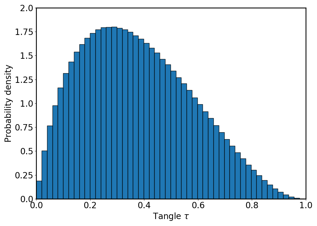
(a)   Tangle

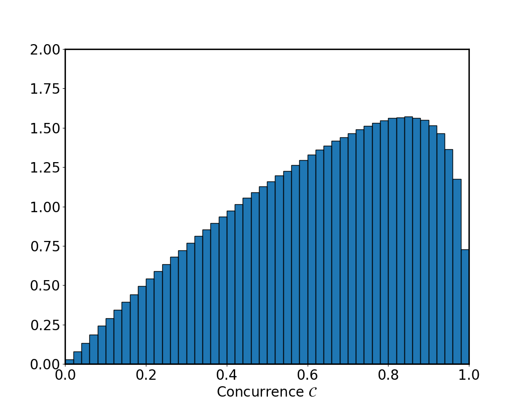
(b)   Concurrence

Figure 1: (a) Probability density of three-qubit random states as a function of the tangle. (b) Probability density of two-qubit random states as a function of the concurrence. Three-qubit random states tend to populate values around $\sim 0.3$, while two-qubit random states are mostly distributed at high values.

In this sense, the canonical representation allows to set several amplitudes of the original state to zero and fix some of its relative phases. A canonical form of a tripartite state such that it respects all its entanglement invariants must be constructed with the use of three local unitaries $U_{A}\otimes U_{B}\otimes U_{C}$, each acting on a partition. For a three-qubit state, the complete rationale for this construction goes as follows. The total number of degrees of freedom of a three-qubit state is $2\times 2^{3}$ real numbers for the coefficients $t_{ijk}$, minus a global phase and norm constraints, which makes a total amount of 14. Now, we remove the freedom carried by the three single-qubit unitaries, which is 3$\times$3. Thus, the number of degrees of freedom is 5. In consequence, there are 5 entanglement invariants under local unitaries Acín et al. (2000). Note that a similar argument applied to $n$ qubits shows that the number of entanglement invariants grows as $2\times 2^{n}-3n-2$.

It is then always possible to bring a three-qubit state to a canonical form, where three amplitudes are set to zero and only one relative phase remains Acín et al. (2000). This canonical form reads

$$|\varphi{\rangle}=\lambda_{0}|000{\rangle}+\lambda_{1}e^{i\phi}|100{\rangle}+\lambda_{2}|101{\rangle}+\lambda_{3}|110{\rangle}+\lambda_{4}|111{\rangle}\,,$$ (4)

where $\{\lambda_{i}\}$ are real positive values and $\phi$ is a relative phase $0\leq\phi\leq\pi$, attached by convention to $|100{\rangle}$. Once the canonical form of the tripartite state is obtained, it is possible to compute the 5 entanglement invariants Sudbery (2001) as

$$\begin{array}[]{l}\frac{1}{2}\leq I_{1}\equiv Tr\,\rho_{A}^{2}=1-2\mu_{0}(1-\mu_{0}-\mu_{1})\leq 1\vspace{0.1cm}\\ \frac{1}{2}\leq I_{2}\equiv Tr\,\rho_{B}^{2}=1-2\mu_{0}(1-\mu_{0}-\mu_{1}-\mu_{2})-2\Delta\leq 1\vspace{0.1cm}\\ \frac{1}{2}\leq I_{3}\equiv Tr\,\rho_{C}^{2}=1-2\mu_{0}(1-\mu_{0}-\mu_{1}-\mu_{3})-2\Delta\leq 1\vspace{0.1cm}\\ \frac{1}{4}\leq I_{4}\equiv Tr\,(\rho_{A}\otimes\rho_{B}\;\rho_{AB})=\\ \phantom{\frac{1}{4}\leq I_{4}=\,}1+\mu_{0}(\mu_{2}\mu_{3}-\mu_{1}\mu_{4}-2\mu_{2}-3\mu_{3}-3\mu_{4})\vspace{0.1cm}\\ \phantom{\frac{1}{4}\leq I_{4}=}-(2-\mu_{0})\Delta\leq 1\vspace{0.1cm}\\ 0\leq I_{5}\equiv|{\rm Hdet}(t_{ijk})|^{2}=\mu_{0}^{2}\mu_{4}^{2}\leq\frac{1}{16}\,,\end{array}$$ (5)

where $\mu_{i}=\lambda_{i}^{2}$ and $\Delta=|\lambda_{1}\lambda_{4}e^{i\phi}-\lambda_{2}\lambda_{3}|^{2}$. Therefore, from Eq. (2) and Eq. (5) follows that

$$\tau=4\,\sqrt{I_{5}}=4\,\mu_{0}\mu_{4}\,.$$ (6)

Consequently, given a state in its canonical form, the tangle can be directly computed as the product of the outcome probabilities of the states $|000{\rangle}$ and $|111{\rangle}$ in the computational basis, multiplied by four.

III Quantum Algorithm for Measuring the Tangle

Let us assume that we receive an unknown three-qubit state $|\psi{\rangle}_{ABC}$. Our goal is to perform local unitary operations on this state in order to transform it to its canonical form in Equation (4). Such operations are defined as

$$|\varphi{\rangle}=U_{A}(\vec{\theta}_{A})\otimes U_{B}(\vec{\theta}_{B})\otimes U_{C}(\vec{\theta}_{C})\,|\psi{\rangle}_{ABC},$$ (7)

where $|\varphi{\rangle}$ is the canonical form of $|\psi{\rangle}_{ABC}$ (we drop the subscript $ABC$ in the canonical form for convenience), and each unitary takes the form

$$U(\vec{\theta})=\begin{pmatrix}\cos\theta_{0}/2&-e^{i\theta_{1}}\sin\theta_{0}/2\\ e^{i\theta_{2}}\sin\theta_{0}/2&e^{i(\theta_{1}+\theta_{2})}\cos\theta_{0}/2\end{pmatrix},$$ (8)

with $\vec{\theta}=(\theta_{0},\theta_{1},\theta_{2})$. It is then necessary to find the values $(\vec{\theta}_{A},\vec{\theta}_{B},\vec{\theta}_{C})_{\rm opt}$ that achieve this transformation. We will follow a hybrid variational strategy and define

$$(\vec{\theta}_{A},\vec{\theta}_{B},\vec{\theta}_{C})_{\rm opt}={\rm argmin}\left(\mathcal{C}(\vec{\theta}_{A},\vec{\theta}_{B},\vec{\theta}_{C})\right)\,,$$ (9)

where $\mathcal{C}$ is the cost function, defined as

$$\mathcal{C}(\vec{\theta}_{A},\vec{\theta}_{B},\vec{\theta}_{C})=\sum_{i}\,|{\langle}i\,|\,U(\vec{\theta}_{A},\vec{\theta}_{B},\vec{\theta}_{C})|\psi_{ABC}{\rangle}\,|^{2},$$ (10)

where $i\in\{001,010,011\}$. Notice that the optimal solution, i.e., the configuration $(\vec{\theta}_{A},\vec{\theta}_{B},\vec{\theta}_{C})_{\rm opt}$ that renders this cost function equal to zero, transforms $|\psi{\rangle}_{ABC}$ into an up-to-phases canonical form $|\tilde{\varphi}{\rangle}$, given by

$$\begin{split}|\tilde{\varphi}{\rangle}=\lambda_{0}|000{\rangle}+\lambda_{1}e^{i\phi_{1}}|100{\rangle}+\lambda_{2}e^{i\phi_{2}}|101{\rangle}+\\ +\lambda_{3}e^{i\phi_{3}}|110{\rangle}+\lambda_{4}e^{i\phi_{4}}|111{\rangle}\,.\end{split}$$ (11)

Such transformation is less restrictive than the canonical transformation in Equation (7). Therefore, there exist many possible optimal parameters. The quantum circuit implementing this operation is depicted in Figure LABEL:fig:local_unitary. Once the optimal parameters are obtained, it is straightforward to measure the tangle $\tau$ in an actual quantum computer. This quantity will be equal to

$$\tau=4\,|{\langle}000|\tilde{\varphi}{\rangle}{\langle}111|\tilde{\varphi}{\rangle}|^{2}=4\,P_{000}P_{111}\,,$$ (12)

where $P_{ijk}$ is the probability of measuring $|ijk{\rangle}$. The statistical additive error of $P_{ijk}$ is given by the sampling process of a multinomial distribution, that is, $\sqrt{P_{ijk}(1-P_{ijk})/M}$, where $M$ is the number of measurements.

We propose a manner to mitigate random errors occurring when computing the tangle, via post-selection. After the optimization is completed, and a low value of the cost function is obtained, it is licit to assume that $|\psi{\rangle}_{ABC}$ has been properly transformed into $|\tilde{\varphi}{\rangle}$. Thus, if the outcome of a measurement is either $|001{\rangle},|010{\rangle}{\rm\,or\,}|011{\rangle}$ after the transformation into the up-to-phases canonical form, it is due to an error in the circuit. In this case, this outcome can be discarded.

$$ IV Simulations The algorithm for measuring the tangle can be benchmarked on simulations. We considered a set of 1000 random states, accounting for finite sampling and noise. The state |GHZ⟩=(|000⟩+|111⟩)/2 has been treated as a particular case, as it is the one that maximizes the tangle and, in addition, it is already in its canonical form. To be precise, we sampled 104 times and introduced random Pauli errors in the quantum circuits in every run, for increasing noise levels. Each measure of the tangle has been repeated ten times, with and without post-selection. We employed the standard Python Library Scipy Virtanen et al. (2020) for the optimization procedure. In particular, we employed the Powell method as it was found to provide accurate results Powell (1964). The mean number of optimization steps is of the order of a few hundred. Not all optimization instances were found to be satisfactory. Some trials did not reach a proper minimum during the first attempt. In order to avoid outliers, only those instances whose cost function was under a certain threshold were accepted. For those that did not match this criterium, the algorithm was rerun. A maximum number of five attempts were allowed. IV.1 Error Model We now present the error model that we have used in the simulations. In this model, single-qubit gates can appear randomly with certain probabilities, to be discussed later. These gates modify the state within the quantum circuit and may appear only after applying the unitary gates from Equation (7). As the algorithm for measuring the tangle does not require the use of entangling gates, we assume that the qubits have no cross-talk, and thus two-qubit errors are omitted. We consider two different types of error. First, random bit-flips, phase-flips and bit-phase-flips are modeled with Pauli-X,Z,and​Y gates respectively. All of them may appear sequentially for each one of the qubits. The second kind of error is measurement errors, which are modeled with a Pauli-X gate appearing just before readout. A scheme for the occurrence of these gates is shown in Figure LABEL:fig:error_model. Every gate has an independent probability of appearing in the circuit, i.e., all error events are uncorrelated. Therefore, the probability of one error ε occurring is Probε=pε​∏e≠ε(1−pe), (13) where pe is the probability that one error occurs, and the product runs over all possible errors. This can be easily extended to calculate the probability of occurrence of a higher number of errors. The probabilities of single-qubit and measurement errors are taken as 0.1​t% and 1​t% respectively, where t={0,1,2,3,4,5} is a tuning parameter. These numbers were selected in agreement with the orders of magnitude present in the experiment in Reference Arute et al. (2019). Considering t=5, there is one error in ∼17% of the samples, and there are ∼1.5% of events with two errors. Three or more errors are unlikely to happen, with appearance rates under 0.1%. As Pauli-X,Y,Z gates do not commute, choosing to apply first one or another is not equivalent. However, the probability of this kind of events is very low. For instance, the probability of two measurement errors is p∼10−4, of one measurement and one single-qubit error is p∼10−5, and for two single-qubit errors is only p∼10−6. Therefore, we choose one particular ordering. Notice as well that the tangle is not affected by some of these errors, such as Pauli-Z errors alone. IV Simulations The algorithm for measuring the tangle can be benchmarked on simulations. We considered a set of 1000 random states, accounting for finite sampling and noise. The state ketGHZket000ket1112 has been treated as a particular case, as it is the one that maximizes the tangle and, in addition, it is already in its canonical form. To be precise, we sampled superscript104 times and introduced random Pauli errors in the quantum circuits in every run, for increasing noise levels. Each measure of the tangle has been repeated ten times, with and without post-selection. We employed the standard Python Library Scipy Virtanen et al. (2020) for the optimization procedure. In particular, we employed the Powell method as it was found to provide accurate results Powell (1964). The mean number of optimization steps is of the order of a few hundred. Not all optimization instances were found to be satisfactory. Some trials did not reach a proper minimum during the first attempt. In order to avoid outliers, only those instances whose cost function was under a certain threshold were accepted. For those that did not match this criterium, the algorithm was rerun. A maximum number of five attempts were allowed. IV.1 Error Model We now present the error model that we have used in the simulations. In this model, single-qubit gates can appear randomly with certain probabilities, to be discussed later. These gates modify the state within the quantum circuit and may appear only after applying the unitary gates from Equation (7). As the algorithm for measuring the tangle does not require the use of entangling gates, we assume that the qubits have no cross-talk, and thus two-qubit errors are omitted. We consider two different types of error. First, random bit-flips, phase-flips and bit-phase-flips are modeled with Pauli-𝑋𝑍and𝑌 gates respectively. All of them may appear sequentially for each one of the qubits. The second kind of error is measurement errors, which are modeled with a Pauli-𝑋 gate appearing just before readout. A scheme for the occurrence of these gates is shown in Figure LABEL:fig:error_model. Every gate has an independent probability of appearing in the circuit, i.e., all error events are uncorrelated. Therefore, the probability of one error 𝜀 occurring is subscriptProb𝜀subscript𝑝𝜀subscriptproduct𝑒𝜀1subscript𝑝𝑒 (13) where subscript𝑝𝑒 is the probability that one error occurs, and the product runs over all possible errors. This can be easily extended to calculate the probability of occurrence of a higher number of errors. The probabilities of single-qubit and measurement errors are taken as 0.1percent𝑡 and 1percent𝑡 respectively, where 𝑡012345 is a tuning parameter. These numbers were selected in agreement with the orders of magnitude present in the experiment in Reference Arute et al. (2019). Considering 𝑡5, there is one error in similar-toabsentpercent17 of the samples, and there are similar-toabsentpercent1.5 of events with two errors. Three or more errors are unlikely to happen, with appearance rates under percent0.1. As Pauli-𝑋𝑌𝑍 gates do not commute, choosing to apply first one or another is not equivalent. However, the probability of this kind of events is very low. For instance, the probability of two measurement errors is similar-to𝑝superscript104, of one measurement and one single-qubit error is similar-to𝑝superscript105, and for two single-qubit errors is only similar-to𝑝superscript106. Therefore, we choose one particular ordering. Notice as well that the tangle is not affected by some of these errors, such as Pauli-𝑍 errors alone. $$