A novel staggered semi–implicit space–time discontinuous Galerkin method for the incompressible Navier-Stokes equations

Abstract

A new high order accurate staggered semi-implicit space–time discontinuous Galerkin (DG) method is presented for the simulation of viscous incompressible flows on unstructured triangular grids in two space dimensions. The staggered DG scheme defines the discrete pressure on the primal triangular mesh, while the discrete velocity is defined on a staggered edge-based dual quadrilateral mesh. In this paper, a new pair of equal-order-interpolation velocity-pressure finite elements is proposed. On the primary triangular mesh (the pressure elements) the basis functions are piecewise polynomials of degree $N$ and are allowed to jump on the boundaries of each triangle. On the dual mesh instead (the velocity elements), the basis functions consist in the union of piecewise polynomials of degree $N$ on the two subtriangles that compose each quadrilateral and are allowed to jump only on the dual element boundaries, while they are continuous inside. In other words, the basis functions on the dual mesh are built by continuous finite elements on the subtriangles. This choice allows the construction of an efficient, quadrature-free and memory saving algorithm. In our coupled space-time pressure correction formulation for the incompressible Navier-Stokes equations, arbitrary high order of accuracy in time is achieved through the use of time-dependent test and basis functions, in combination with simple and efficient Picard iterations. Several numerical tests on classical benchmarks confirm that the proposed method outperforms existing staggered semi-implicit space-time DG schemes, not only from a computer memory point of view, but also concerning the computational time.

1 Introduction

In this article we propose a new pair of velocity-pressure elements in the framework of the family of arbitrary high-order accurate staggered semi-implicit space–time Discontinuous Galerkin (DG) methods for the two-dimensional incompressible Navier-Stokes equations on unstructured meshes, extending the works in STINS2D ; STINS2DTri by Tavelli and Dumbser.
The discretization of the incompressible Navier-Stokes equations was mainly carried out in the past using finite difference methods markerandcell ; patankar ; patankarspalding ; vanKan or continuous finite element schemes SUPG ; Fortin ; Rannacher1 ; Rannacher3 ; SUPG2 ; TaylorHood ; Verfuerth . While until a few years ago finite volume methods were more popular, nowadays DG schemes, first introduced by Reed and Hill in reed , are now widely applied in several different fields. In a collection of seminal works cbs3 ; cbs2 ; cbs1 ; cbs0 ; cbs4 , Cockburn and Shu provided a rigorous formulation of these methods, contributing to their widespread use nowadays. For their applications to the Navier-Stokes equations, let us mention the pioneering works of Bassi and Rebay BassiRebay , and Baumann and Oden Baumann199979 . Later, several high order DG methods for the incompressible and compressible Navier-Stokes equations have been proposed, see for example Bassi2006 ; Bassi2007 ; Crivellini2013 ; DumbserNSE ; Ferrer2011 ; MunzDiffusionFlux ; HartmannHouston1 ; HartmannHouston2 ; KleinKummerOberlack2013 ; Nguyen2011 ; Rhebergen2012 ; Rhebergen2013 ; Shahbazi2007 .
The typical saddle point problem of the incompressible Navier-Stokes equations is conveniently managed through the well-known semi-implicit technique on staggered meshes introduced by Harlow and Welch in markerandcell . Further related semi-implicit methods were developed for the incompressible Navier-Stokes equations in Bell1989 ; chorin1 ; chorin2 ; HirtNichols ; patankar ; vanKan . For asymptotic preserving semi-implicit schemes, also in the context of all Mach number flow solvers, see e.g. KleinMach ; Munz2003 ; ParkMPV ; CordierDegond ; DumbserCasulli2016 ; RussoSI ; RussoSI2 ; RussoAllMach .

A whole family of staggered finite difference methods for free-surface flows has been developed in the last decades by Casulli et al., see Casulli2009 ; CasulliVOF ; casulli:1984 ; CasulliStelling2011 ; CasulliWalters2000 . A theoretical analysis of this approach can be found in BrugnanoCasulli ; BrugnanoCasulli2 ; BrugnanoSestini ; CasulliCattani ; CasulliCheng1992 ; CasulliZanolli2012 . All of the mentioned works are characterized by the property that the nonlinear convective terms are discretized explicitly, while the pressure terms are discretized implicitly. Thanks to their high computational efficiency, these methods have been extended to many different applications in science and engineering: let us mention for example blood flow in compliant vessels CasulliDumbserToro2012 ; FambriDumbserCasulli or compressible gas dynamics in elastic tubes DumbserIbenIoriatti . The first direct extension of staggered semi-implicit schemes to the DG framework has been derived in DumbserCasulli ; 2DSIUSW for the shallow water equations on Cartesian and unstructured triangular grids, respectively. The resulting staggered semi-implicit DG method has furthermore been extended to the incompressible and compressible Navier-Stokes equations in two and three space dimensions, see FambriDumbser ; STINS2D ; STINS2DTri ; STINS3D ; STCNS , thus constituting a solid and well-established starting point for our research.
In our staggered approach, the spatial discretization is performed through the use of two unstructured grids: a primary triangular grid for the discrete pressure, and a dual edge-based quadrilateral grid for the discrete velocity, see also Bermudez1998 ; Bermudez2014 ; USFORCE ; USFORCE2 . While the use of staggered grids is a very common practice in the finite difference and finite volume framework (see e.g. casulli:1984 ; markerandcell ; patankarspalding ), its use is not so common in the framework of DG methods. The first vertex-based staggered DG schemes were proposed in CentralDG1 ; CentralDG2 . Other recent edge-based staggered DG schemes have been proposed in StaggeredDGCE1 ; StaggeredDG . The main advantage of using edge-based staggered grids is the sparsity pattern of the final linear system that has to be solved for the pressure. Alternatively, semi-implicit DG schemes on collocated grids have been presented, for example, in Dolejsi1 ; Dolejsi2 ; Dolejsi3 ; GiraldoRestelli ; TumoloBonaventuraRestelli .
Another consequence of the use of a staggered formulation is that, since all quantities are readily defined where they are needed, we do not need any Riemann solvers (numerical flux functions), apart from the nonlinear convective terms. This special feature is not standard for DG schemes, which typically require numerical fluxes or penalty terms, see CBS-convection-diffusion ; CBS-convection-dominated ; MunzDiffusionFlux ; YanShu . For the nonlinear convective part of the incompressible Navier-Stokes equations, we use a standard DG scheme based on the Rusanov flux Rusanov:1961a . Also the viscous terms are discretized explicitly. The DG discretization of the viscous fluxes is based on the formulation of Gassner et al. MunzDiffusionFlux , which was developed for the solution of the Generalized Riemann Problem (GRP) of the diffusion equation.
The introduction of our new pair of quadrature-free equal-order-interpolation velocity-pressure elements has the objective to reduce memory requirements and CPU cost of the previous staggered-semi-implicit DG schemes introduced in STINS2D ; STINS3D . While the scheme presented in this paper is still limited to fixed meshes (Eulerian approach), the proposed quadrature-free formulation has also the potential to be extended to moving unstructured meshes in the Arbitrary-Lagrangian-Eulerian (ALE) context in the future. A lot of research about Lagrangian methods has been carried out in the last decades Benson1992a ; Caramana1998 ; Despres2009 ; Maire2007 ; munz94 ; vonneumann50 ; Smith1999 , due to their excellent properties in the resolution of moving material interfaces and contact waves. In ALE schemes, see e.g. Feistauer4 ; Feistauer1 ; Feistauer3 ; Feistauer2 ; Hirt74 ; Peery2000 ; Smith1999 , the computational grid moves with an arbitrary mesh velocity that does not necessarily coincide with the real fluid velocity. For some examples of the so-called indirect cell-centered ALE algorithms, the reader is referred to MaireMM2 ; ShashkovRemap1 ; ShashkovRemap5 ; ShashkovRemap3 ; ShashkovRemap4 ; ShashkovCellCentered . Many multi-phase and multi-material flow problems are solved relying on this approach ShashkovMultiMat3 ; ShashkovMultiMat1 ; Hirt74 ; Peery2000 ; ShashkovMultiMat4 ; Smith1999 ; ShashkovMultiMat2 . In a recent series of works ALEMQF ; LagrangeMDRS ; Lagrange2D ; Lagrange3D ; LagrangeDG ; LagrangeQF ; LagrangeMHD ; ALELTS2D ; ALEMOOD2 ; ALEMOOD1 ; ALELTS1D ; Lagrange1D ; KlingenALE2017 , a new family of high order accurate finite volume and DG schemes has been proposed in the ALE framework.
The rest of the paper is organized as follows. In Section 2, we briefly introduce the notation for the Navier-Sokes equations; Section 3 is dedicated to the presentation of the new staggered space-time discontinuous Galerkin finite elements; in Section 4 we provide a detailed description of the final solving algorithm; and in Section 5 the validation and the performance analysis of the method are illustrated through several numerical tests.

2 The governing equations

The conservative form of the Navier-Stokes equations for an incompressible Newtonian fluid with constant density $\rho$ and constant dynamic viscosity coefficient $\mu$ in the domain $\Omega\subset\mathds{R}^{d}$ read as follows:

$$\nabla\cdot\mathbf{v}=0,,$$ (1)

$$\frac{\partial\mathbf{v}}{\partial t}+\nabla\cdot\mathbf{F}_{c}+\nabla p=\nabla\cdot\left(\nu\nabla\mathbf{v}\right)+\mathbf{S},$$ (2)

where $\mathbf{v}=\left(u,v\right)^{T}$ is the velocity vector, $u$ and $v$ are the velocity components in the $x$ and $y$ direction, respectively, $\mathbf{F}_{c}=\mathbf{v}\otimes\mathbf{v}$ is the flux tensor containing the nonlinear convective terms, and which in two space dimensions reads

$$\mathbf{F}_{c}=\left(\begin{array}[]{cc}u^{2}&uv\\ uv&v^{2}\end{array}\right);$$

then $p=P/\rho$ is the normalized fluid pressure, $P$ is the physical pressure, $\nu=\mu/\rho$ is the kinematic viscosity coefficient and, finally, $\mathbf{S}=\mathbf{S}(\mathbf{v},x,y,t)$ is a generic source term representing the volumetric forces.
Following the same idea of DumbserNSE ; MunzDiffusionFlux , the viscosity term is grouped together with the nonlinear convective term. In this way the momentum equation (2) can be rewritten as:

$$\frac{\partial\mathbf{v}}{\partial t}+\nabla\cdot\mathbf{F}_{cv}+\nabla p=\mathbf{S},$$ (3)

where $\mathbf{F}_{cv}=\mathbf{F}_{cv}(\mathbf{v},\nabla\mathbf{v})=\mathbf{F}_{c}(\mathbf{v})-\nu\nabla\mathbf{v}$ is a nonlinear tensor that depends not only on the velocity, but also on its gradient:

$$\mathbf{F}_{cv}=\left(\begin{matrix}u^{2}-\nu\frac{\partial{u}}{\partial{x}}&uv-\nu\frac{\partial{u}}{\partial{y}}\\ uv-\nu\frac{\partial{v}}{\partial{x}}&v^{2}-\nu\frac{\partial{v}}{\partial{y}}\end{matrix}\right).$$

For a clear presentation of our numerical method, which involves a weak space–time formulation of the Navier-Stokes equations, we restyle equations (1) and (3) in the following equivalent, but more compact, form:

$$\tilde{\nabla}\cdot\tilde{\mathbf{v}}=0,$$ (4)

$$\tilde{\nabla}\cdot\tilde{\mathbf{F}}_{cv}+\tilde{\nabla}\cdot\tilde{\mathbf{F}}_{p}=\mathbf{S},$$ (5)

by introducing the space–time divergence operator $\tilde{\nabla}=\left(\frac{\partial{}}{\partial{t}},\frac{\partial{}}{\partial{x}},\frac{\partial{}}{\partial{y}}\right)^{T}$, the vector $\tilde{\mathbf{v}}=\left(0,u,v\right)^{T}$ and the tensors:

$$\tilde{\mathbf{F}}_{cv}=\left(\begin{matrix}u&u^{2}-\nu\frac{\partial{u}}{\partial{x}}&uv-\nu\frac{\partial{u}}{\partial{y}}\\ v&uv-\nu\frac{\partial{v}}{\partial{x}}&v^{2}-\nu\frac{\partial{v}}{\partial{y}}\end{matrix}\right),\quad\tilde{\mathbf{F}}_{p}=\left(\begin{matrix}0&p&0\\ 0&0&p\end{matrix}\right).$$ (6)

3 The new staggered space–time basis functions

The main novelty of our new numerical method with respect to previous similar work presented in STINS2D ; STINS2DTri consists in the use of a different kind of finite elements in the framework of a staggered space-time DG method. An edge-based staggered approach for two-dimensional domains is considered, see Bermudez1998 ; StaggeredDG ; 2DSIUSW ; STINS2D ; STINS2DTri ; STCNS ; USFORCE , but here we propose a new pair of finite elements that is in principle also suitable for staggered ALE methods for the incompressible Navier-Stokes equations on moving meshes.
In paragraph 3.1 we briefly summarize the used notation; then paragraphs 3.2 and 3.3 illustrate the spatial and the temporal discretization of the problem, respectively, and, finally, the space–time finite elements are defined in paragraph 3.4.

3.1 Unstructured staggered grids

Let us consider the domain of the problem $\Omega\subset\mathbb{R}^{2}$ and its boundary $\partial\Omega$. For a graphical illustration of the following discussion, the reader is addressed to Figure 1.
The computational domain $\Omega_{h}$ is covered with a triangulation $\mathcal{T}_{h}$ of $N_{e}$ non-overlapping triangular elements, denoted by $T_{i}$:

$$\Omega_{h}=\bigcup_{i=1,\ldots,N_{e}}{T}_{i}\>.$$

Let $N_{d}$ be the total number of edges of the triangles, and let us call $\Gamma_{j}$ the $j-$th edge of the primary grid, with $j=1,\ldots,N_{d}$. The subset of edges $\mathcal{B}(\Omega_{h})$ is defined as the set of the indices $j$ corresponding to the boundary edges:

$$\mathcal{B}(\Omega_{h})=\{j\in[1,N_{d}]:\Gamma_{j}\subset\partial\Omega\}.$$

For every $i=1,\ldots,N_{e}$, we denote by $S_{i}$ the set of the three edges belonging to triangle ${T}_{i}$:

$$S_{i}=\{j\in[1,N_{d}]:\Gamma_{j}\subset\partial{T}_{i}\}\quad\Rightarrow\quad|S_{i}|=3.$$

For every internal edge with index $j\in[1,N_{d}]\setminus\mathcal{B}(\Omega_{h})$, the corresponding dual quadrilateral element is called ${R}_{j}$ and is built by taking as vertices the two barycenters of the triangles sharing the edge (the one on the left is called ${T}_{l(j)}$ and the one on the right is called ${T}_{r(j)}$) and the two vertices of $\Gamma_{j}$.
Let us denote by ${T}_{i,j}={R}_{j}\cap{T}_{i}$ the sub-triangle which is in common between element ${T}_{i}$ and element ${R}_{j}$, for every $i=1,\ldots,N_{e}$ and for every $j\in S_{i}$. Notice that, if $j\in\mathcal{B}(\Omega_{h})$, then a special triangular element ${R}_{j}$ will be part of the dual staggered grid: it is defined by the two vertices of $\Gamma_{j}$ and the barycenter of triangle ${T}_{i}$, with $j\in S_{i}$. In particular, in this case they are equivalent: ${R}_{j}={T}_{i,j}\>.$

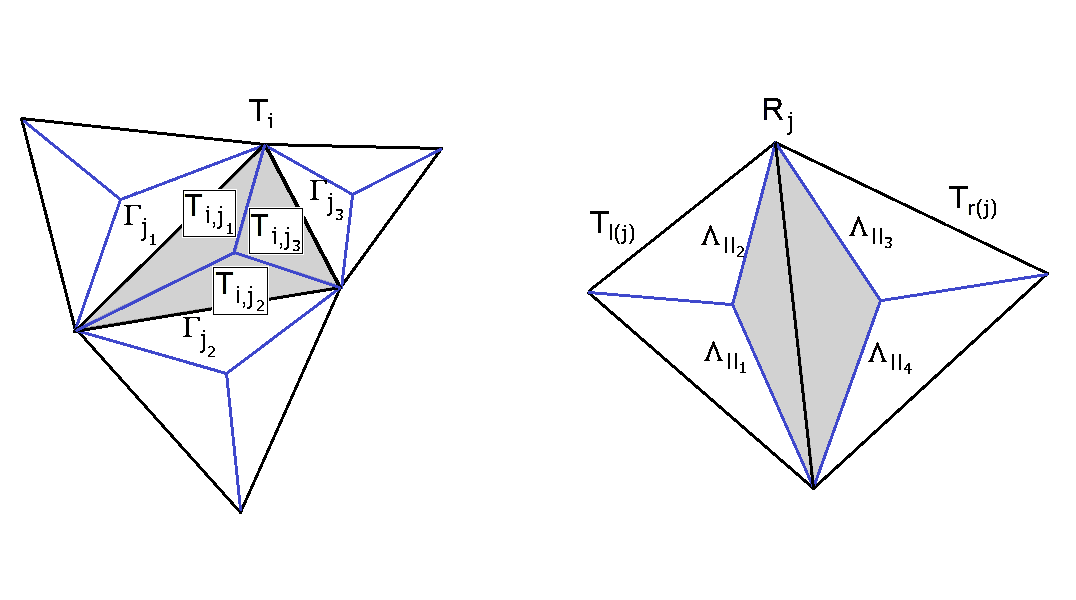
Figure 1: The notation used for the primary triangular mesh (on the left) and for the associated dual quadrilateral mesh (on the right).

According to STINS2D , the mesh of triangular elements $\{{T}_{i}\}_{i\in[1,N_{e}]}$ is called the main grid or primary grid and will be used for the approximation of the pressure $p_{h}$, while the set of the elements $\{{R}_{j}\}_{j\in[1,N_{d}]}$ is called the dual grid and will be used for the approximation of the velocity $\mathbf{v}_{h}$.
The notation for the analogous quantities of the dual grid is the following: $N_{l}$ indicates the total number of edges; $\Lambda_{ll}$ indicates the $ll$-th physical edge; and for every $j=1,\ldots,N_{d}$, we denote by $E_{j}$ the set of the edges belonging to element ${R}_{j}$:

$$E_{j}=\{ll\in[1,N_{l}]:\Lambda_{ll}\subset\partial{R}_{j}\}\quad\Rightarrow\quad\begin{cases}|E_{j}|=4\quad\text{if }j\notin\mathcal{B}(\Omega_{h})\\ |E_{j}|=3\quad\text{if }j\in\mathcal{B}(\Omega_{h})\end{cases}.$$

3.2 Spatial basis functions

As usual in the framework of finite element methods, we first define the basis functions on a reference element and then we can extend them to the physical space of the whole computational domain. We employ the standard nodal or ”Lagrangian” approach for the definition of the basis functions.

For the primary finite element space of polynomial approximation degree $N$, let us define the triangular reference element

$$T_{std}=\{(\xi,\eta)\in\mathbb{R}^{2,+}:\eta\leq 1-\xi\wedge 0\leq\xi\leq 1\},$$

and let us impose the classical Lagrange interpolation condition $\phi_{k}(\vec{\xi}_{l})=\delta_{kl}$ over the nodal points:

$$\vec{\xi}_{k}=(\xi_{k_{1}},\eta_{k_{2}})=\left(\frac{k_{1}}{N},\frac{k_{2}}{N}\right),$$ (7)

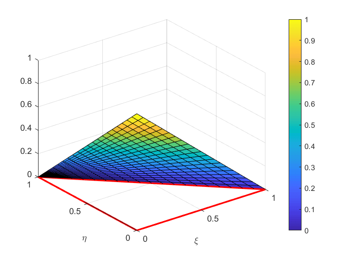
(a) $\phi_{1}(\xi,\eta)$

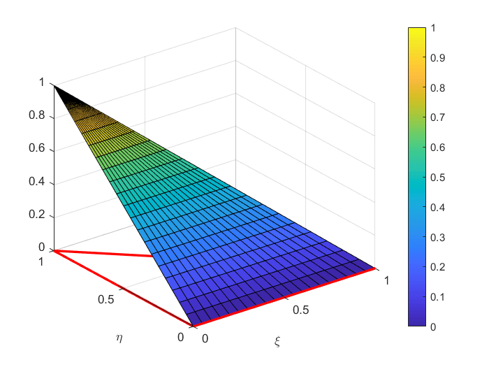
(b) $\phi_{2}(\xi,\eta)$

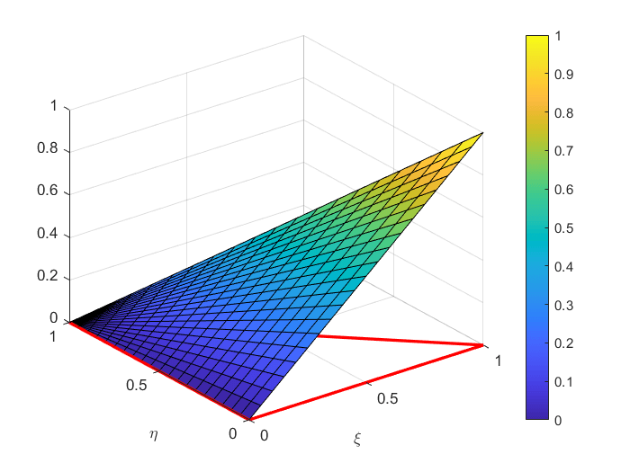
(c) $\phi_{3}(\xi,\eta)$

Figure 2: The $N=1$ basis functions of the primary grid.

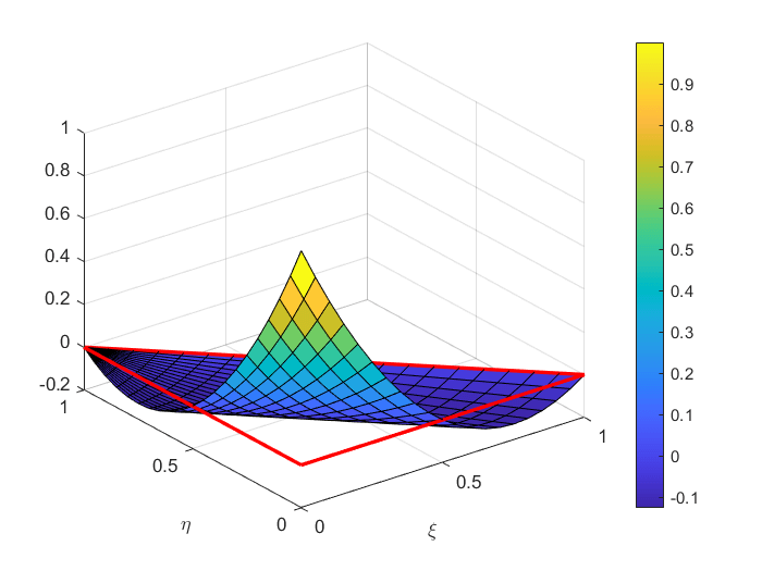
(a) $\phi_{1}(\xi,\eta)$

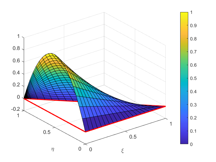
(b) $\phi_{2}(\xi,\eta)$

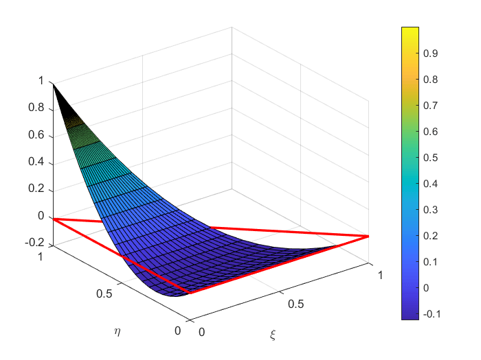
(c) $\phi_{3}(\xi,\eta)$

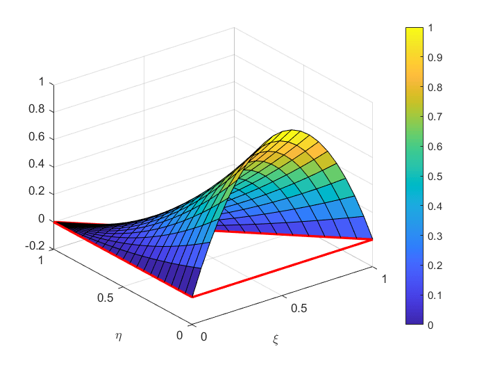
(d) $\phi_{4}(\xi,\eta)$

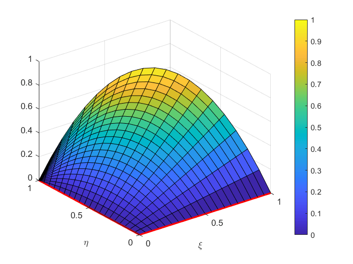
(e) $\phi_{5}(\xi,\eta)$

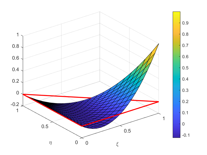
(f) $\phi_{6}(\xi,\eta)$

Figure 3: The $N=2$ basis functions of the primary grid.

where $\delta$ indicates the Kronecker delta, $k=(k_{1},k_{2})$ is a multi-index and the ranges for indices $k_{1}$, $k_{2}$ are $0\leq k_{1}\leq N$ and $0\leq k_{2}\leq N-k_{1}$. In total, $N_{\phi}=\frac{(N+1)(N+2)}{2}$ basis functions are obtained for the reference element of the primary grid and they are labeled as $\{\phi_{k}\}_{k\in[1,N_{\phi}]}$. A visualization of them can be found in Figure 2 for $N=1$ and in Figure 3 for $N=2$.

Similarly, for the dual finite element space of polynomial approximation degree $N$, one could obtain another set of nodal basis functions on the reference square element

$$R_{std}=\{(\xi,\eta)\in\mathbb{R}^{2,+}:0\leq\xi\leq 1\wedge 0\leq\eta\leq 1\}$$

with the nodes given by the tensor product of $N+1$ one-dimensional quadrature points, for example the Newton-Cotes ones, see stroud , as it was done in STINS2D ; STINS2DTri . Instead, in this paper we define the basis functions on $R_{std}$ in a different way, using the continuous union of piecewise polynomials of degree $N$ defined on each of the two subtriangles which constitute the reference square. Let us consider the square $R_{std}$ as the union of two sub-triangles $T_{I}$ and $T_{II}$, with $T_{I}=T_{std}$, and let us define the new basis functions following the standard nodal approach of conforming continuous finite elements with order $N$ inside the square ($T_{I}$ and $T_{II}$ are the so called ”mini-elements”). This is an approach very similar to the $\mathbb{P}^{k}-\text{iso}\mathbb{P}^{k+1}$ finite elements, described in ern2004 , which are applied for the velocity approximation in some mixed problems (for example the Stokes problem, where mixed finite element approximations are employed in order to numerically satisfy the inf-sup or Ladyzhenskaya-Babuška-Brezzi compatibility condition). But, instead of creating new elements inside a triangular macro-element, in our staggered approach the macro-element is given by the square, and the two mini-elements naturally arise from the edge-staggered geometric configuration.
In other words, we build the basis functions over the nodes which lie on sub-triangle $T_{I}$ exactly like we did for $T_{std}$, and then we extend them to $T_{II}$ with zero, in order to mantain the continuity inside the square. Viceversa, we define the basis functions over the nodes which lie on $T_{II}$ via the transformation $\sigma_{(\frac{1}{2},\frac{1}{2})}$ between $T_{II}$ and $T_{I}$, and then we extend them continuously to $T_{I}$ with zero. Here, $\sigma_{(\frac{1}{2},\frac{1}{2})}$ indicates the central symmetry with center $\left(\frac{1}{2},\frac{1}{2}\right)$ in the $\xi-\eta$ plane. In conclusion, $N_{\psi}=(N+1)^{2}$ basis functions are generated for the dual grid, i.e. for the spatial discretization of the velocity components, and they are labelled as $\{\psi_{k}\}_{k\in[1,N_{\psi}]}$. Their formal piecewise definition is as follows.

1. If $1\leq k\leq\frac{N(N+1)}{2}$ ,

   $$\psi_{k}(\vec{\xi})=\begin{cases}\phi_{k}(\vec{\xi})\quad&\text{if }\vec{\xi}\in T_{I}\\ 0\quad&\text{if }\vec{\xi}\in T_{II}\end{cases}\>;$$ (8)

2. if $\frac{N(N+1)}{2}<k\leq N_{\phi}$ ,

   $$\psi_{k}(\vec{\xi})=\begin{cases}\phi_{k}(\vec{\xi})\quad&\text{if }\vec{\xi}\in T_{I}\\ \phi_{(N+1)^{2}-(k-1)}\left(\sigma_{(\frac{1}{2},\frac{1}{2})}(\vec{\xi})\right)\quad&\text{if }\vec{\xi}\in T_{II}\end{cases}\>;$$ (9)

3. if $N_{\phi}<k\leq N_{\psi}$ ,

   $$\psi_{k}(\vec{\xi})=\begin{cases}0\quad&\text{if }\vec{\xi}\in T_{I}\\ \phi_{k-N_{\phi}}\left(\sigma_{(\frac{1}{2},\frac{1}{2})}(\vec{\xi})\right)\quad&\text{if }\vec{\xi}\in T_{II}\end{cases}\>.$$ (10)

A plot of them is available in Figure 4 for the case $N=1$ and in Figure 6 for the case $N=2$. A comparison with the old basis functions used in STINS2D ; STINS2DTri can be found in Figures 5 and 7.

One clear advantage of this choice, from the programming point of view, is that the basis functions for the dual grid can be obtained by a simple manipulation of the basis functions of the primary grid. Indeed, notice that the primary grid and the dual grid have got the same degree of interpolation $N$. For this reason, we call this new pair of finite elements equal-order-interpolation velocity-pressure elements.
Another crucial point is that the new velocity-pressure elements are in principle also suitable for an ALE implementation of a numerical solver, in which two important issues are the RAM memory required by the simulations and the computational time spent by the updating of the matrices in the overall algorithm. One of the purposes of this paper is to show that the ALE (moving meshes) implementation of our high-order accurate staggered numerical method with the new pair of velocity-pressure elements yields even better performance compared with the Eulerian (fixed mesh) implementation of the original method STINS2DTri , concerning the two above-mentioned aspects. The performance comparisons of the two versions of the numerical solver are reported in detail in Section 5.
The improved performace of the new method are indeed possible thanks to the new piecewise definition of the dual basis functions for the definition of the discrete velocity. As it will be clear when looking at the algebraic formulation of the problem (Paragraph 4.2), all the matrices of the final system to be solved are related to one and only one subset of the dual basis functions, hence to one and only one of the definitions in Formulae (8), (9), (10), namely: (i) the basis functions associated to the nodes of the left sub-triangle $T_{I}$, or (ii) the basis functions associated to the nodes belonging to the diagonal of $R_{std}$ connecting the points $(0,1)$ and $(1,0)$, or (iii) the basis functions associated to the nodes of the right sub-triangle $T_{II}$. It turns out that two great advantages are achieved.
First, given the approximation degree $N$, only a relatively small, constant number of universal matrices computed over the $T_{std}$ reference element (for the volume space–time integral matrices), or over the unit interval $I_{std}=[0,1]$ (for the surface space–time integral matrices) are needed to be stored by the program. This means that only a universal version of the matrices and not all the local matrices must be stored, therefore the new velocity-pressure elements allow to save a great amount of RAM memory, especially for simulations employing very refined meshes.
Secondly, the task of updating all the local matrices at each time step in the ALE algorithm is carried out through a simple tensor-reduction operation, where the local matrices are computed on the fly from the universal matrices and from the geometric information of the moving meshes. Of course, this operation is much faster than recomputing from scratch all the integrals of the matrices, and the advantage in terms of computational time is significant when employing high-order finite elements, which would require very expensive numerical quadrature formulae in the recalculation of the matrices for every time step of the ALE simulation.

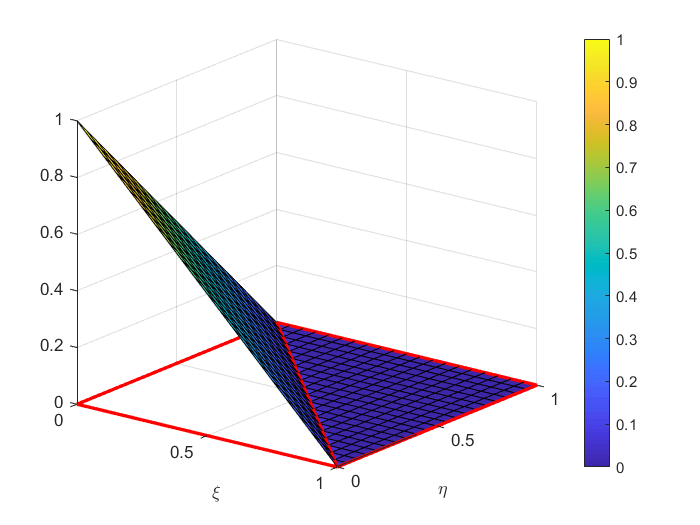
(a) $\psi_{1}(\xi,\eta)$

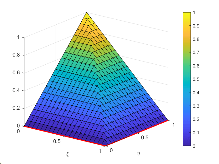
(b) $\psi_{2}(\xi,\eta)$

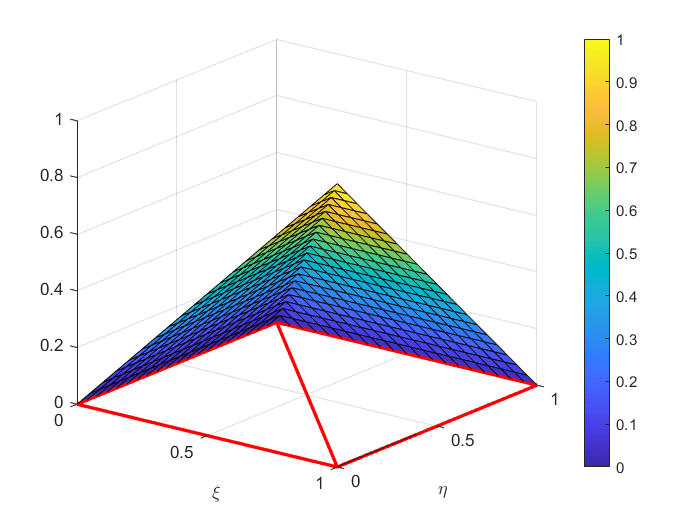
(c) $\psi_{3}(\xi,\eta)$

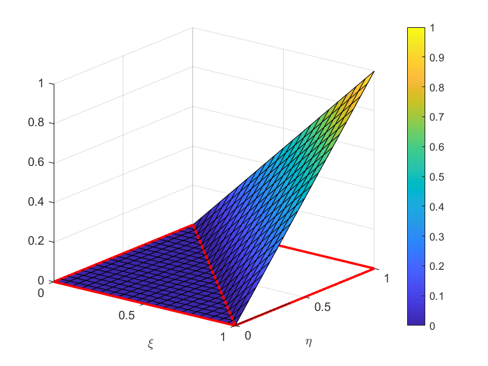
(d) $\psi_{4}(\xi,\eta)$

Figure 4: The new $N=1$ basis functions of the dual grid proposed in this paper.

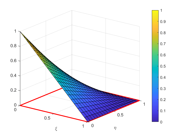
(a) $\psi_{1}(\xi,\eta)$

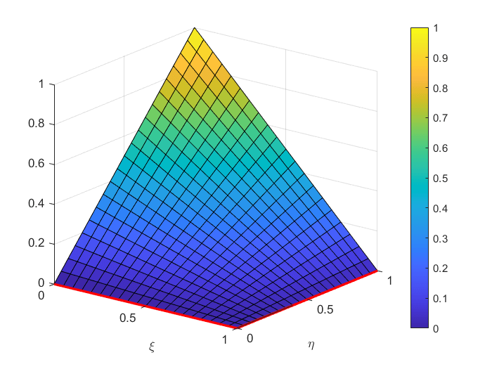
(b) $\psi_{2}(\xi,\eta)$

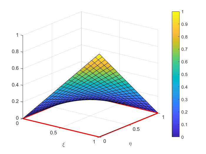
(c) $\psi_{3}(\xi,\eta)$

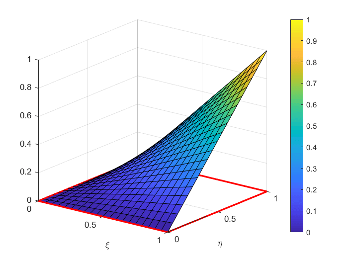
(d) $\psi_{4}(\xi,\eta)$

Figure 5: The previous $N=1$ basis functions on the dual grid used in STINS2D ; STINS2DTri .

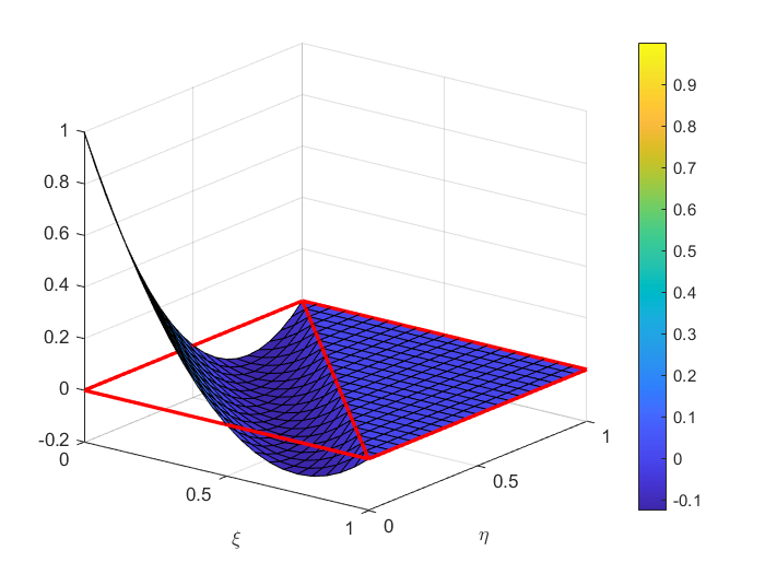
(a) $\psi_{1}(\xi,\eta)$

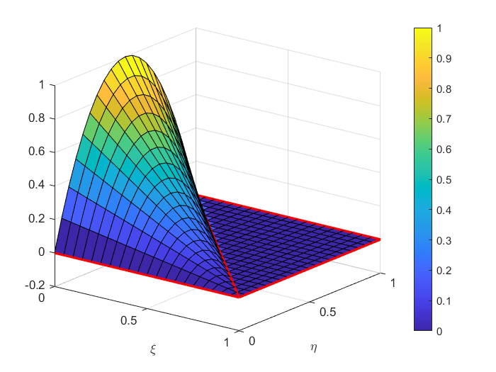
(b) $\psi_{2}(\xi,\eta)$

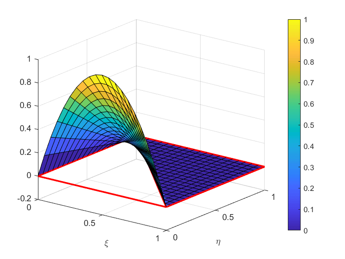
(c) $\psi_{3}(\xi,\eta)$

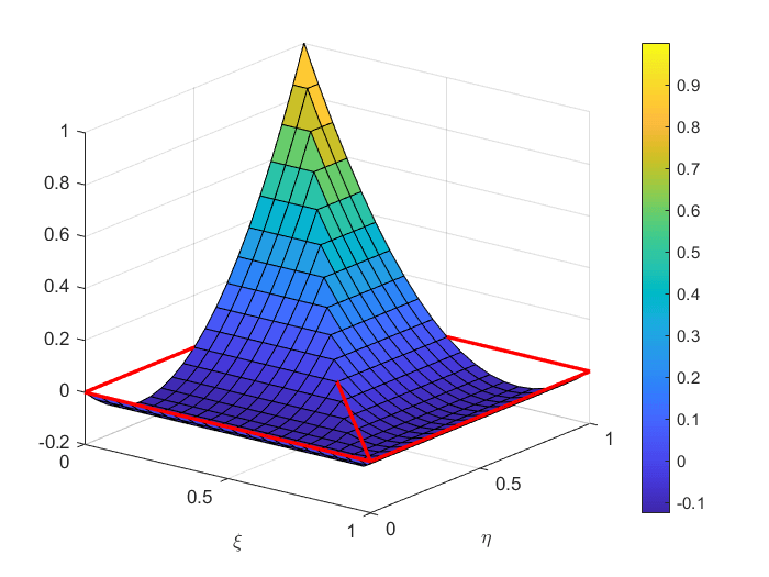
(d) $\psi_{4}(\xi,\eta)$

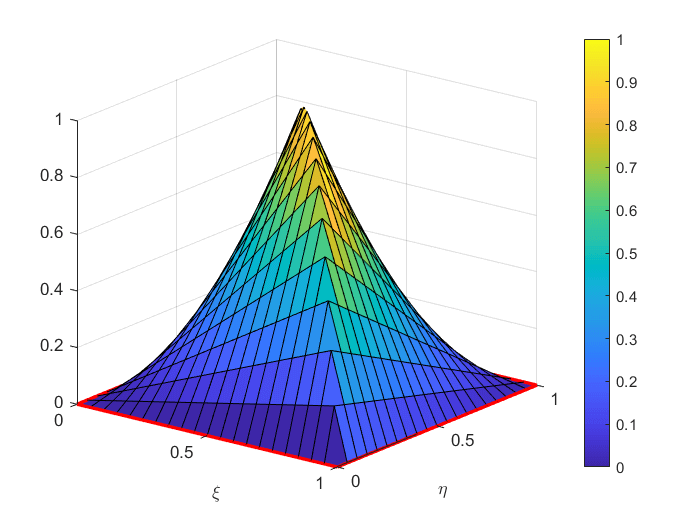
(e) $\psi_{5}(\xi,\eta)$

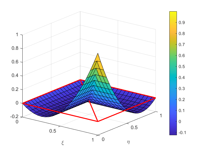
(f) $\psi_{6}(\xi,\eta)$

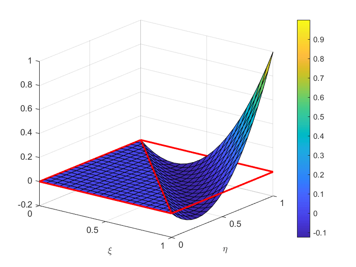
(g) $\psi_{7}(\xi,\eta)$

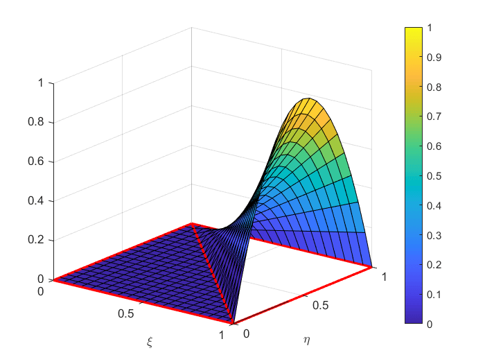
(h) $\psi_{8}(\xi,\eta)$

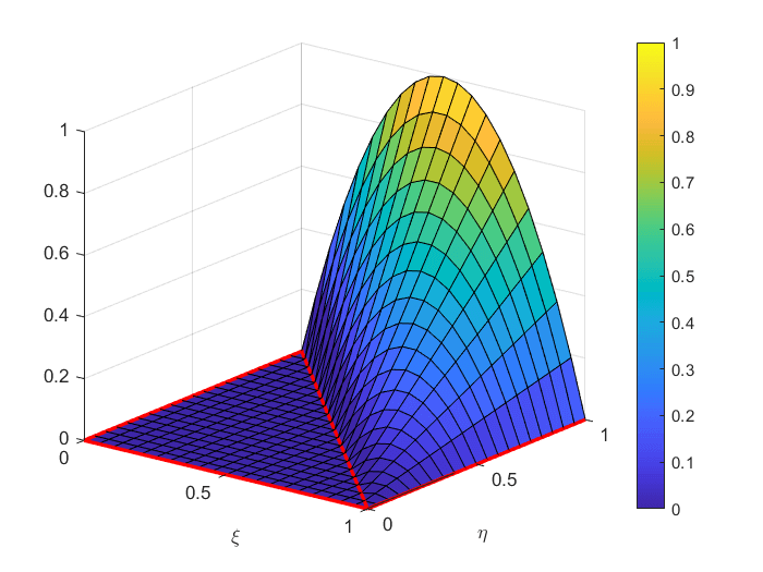
(i) $\psi_{9}(\xi,\eta)$

Figure 6: The new $N=2$ basis functions of the dual grid proposed in this paper.

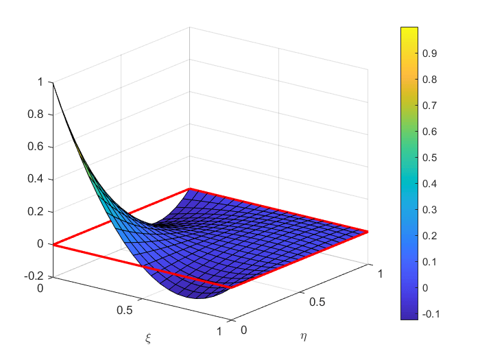
(a) $\psi_{1}(\xi,\eta)$

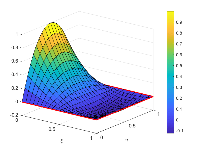
(b) $\psi_{2}(\xi,\eta)$

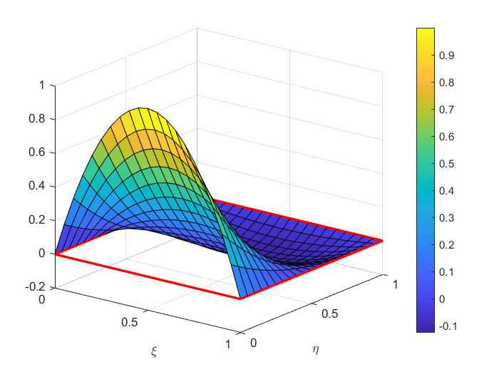
(c) $\psi_{3}(\xi,\eta)$

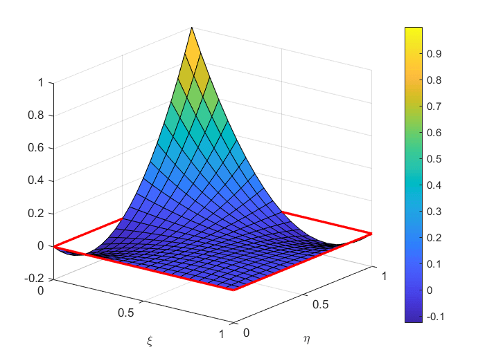
(d) $\psi_{4}(\xi,\eta)$

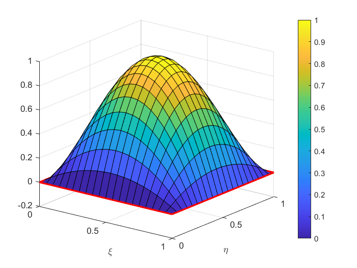
(e) $\psi_{5}(\xi,\eta)$

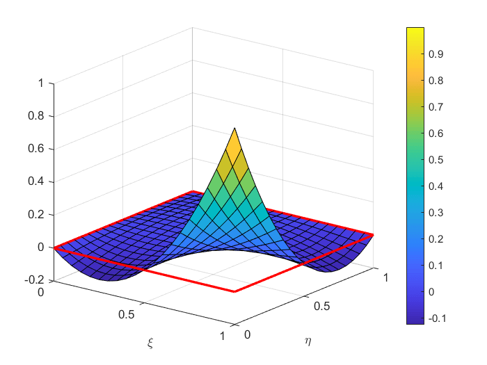
(f) $\psi_{6}(\xi,\eta)$

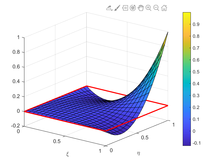
(g) $\psi_{7}(\xi,\eta)$

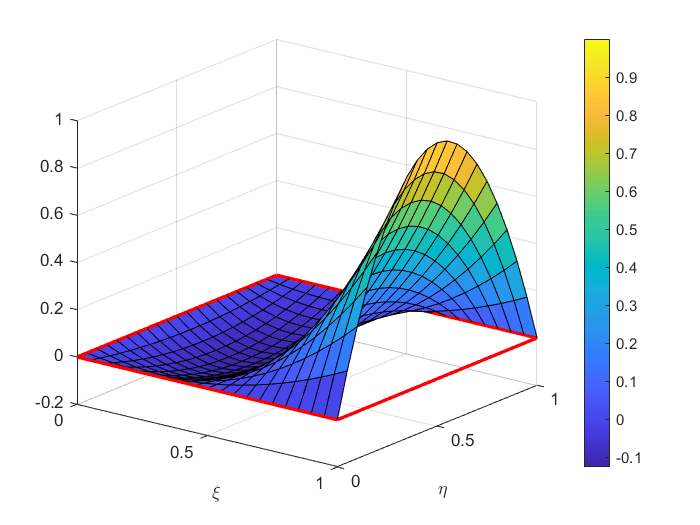
(h) $\psi_{8}(\xi,\eta)$

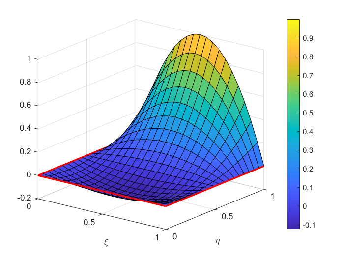
(i) $\psi_{9}(\xi,\eta)$

Figure 7: The previous $N=2$ basis functions on the dual grid used in STINS2D ; STINS2DTri .

3.3 Extension to the space–time basis functions

Since we apply high-order accurate methods also in time, our numerical scheme described in Section 4, is of the kind of the space–time DG schemes, see e.g. KlaijVanDerVegt ; Rhebergen2013 ; spacetimedg1 ; spacetimedg2 . Following STINS2DTri ; STCNS ; STDGLE , we have to define the space–time basis functions as an extension of the spatial basis functions introduced in the previous paragraph.
If the time interval of our problem starts at instant $0$ and ends at instant $T$, we define a number of $N_{t}$ timesteps over the sequence of times:

$$0=t^{0}<t^{1}<t^{2}<\ldots<t^{N_{t}}=T,$$

and we use the notation $T^{n+1}=[t^{n},t^{n+1}]$ for the time interval and $\Delta t^{n+1}=t^{n+1}-t^{n}$ for the timestep length, for each $n=0,\ldots,N_{t}-1$.
For polynomials of degree $p_{\gamma}$, let us define the temporal basis functions on the reference interval $I_{std}=[0,1]$ as the Lagrange interpolation polynomials passing through the equidistant 1D Newton-Cotes quadrature nodes stroud . The resulting $N_{\gamma}=p_{\gamma}+1$ basis functions are labelled as $\{\gamma_{k}\}_{k\in[1,N_{\gamma}]}$. A plot of them can be found in Figures 8 and 9, for the cases $p_{\gamma}=1$ and $p_{\gamma}=2$, respectively.

(a) $\gamma_{1}(\tau)$

(b) $\gamma_{2}(\tau)$

Figure 8: The $p_{\gamma}=1$ basis functions on $I_{std}$.

(a) $\gamma_{1}(\tau)$

(b) $\gamma_{2}(\tau)$

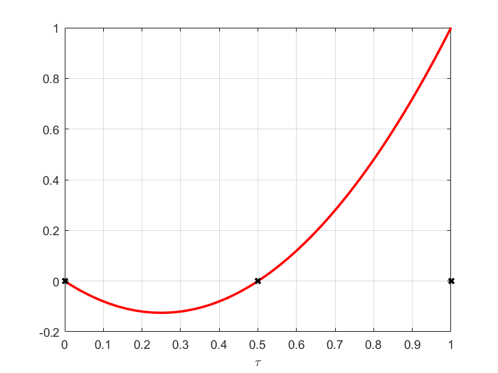
(c) $\gamma_{3}(\tau)$

Figure 9: The $p_{\gamma}=2$ basis functions on $I_{std}$.

Using the tensor product between the new spatial basis functions introduced in the previous paragraph and the temporal basis functions, we can define the basis functions on the space–time reference elements $T_{std}^{st}=T_{std}\times I_{std}$ and $R_{std}^{st}=R_{std}\times I_{std}$ as:

$$\tilde{\phi}_{k}(\xi,\eta,\tau)=\phi_{m_{1}(k)}(\xi,\eta)\cdot\gamma_{m_{2}(k)}(\tau)\quad\forall k=1,\ldots,N_{\phi}^{st}$$ (11)

and

$$\tilde{\psi}_{k}(\xi,\eta,\tau)=\psi_{d_{1}(k)}(\xi,\eta)\cdot\gamma_{d_{2}(k)}(\tau)\quad\forall k=1,\ldots,N_{\psi}^{st},$$ (12)

having defined $N_{\phi}^{st}=N_{\phi}\cdot N_{\gamma}$, $N_{\psi}^{st}=N_{\psi}\cdot N_{\gamma}$ and the sub-indices $m_{1}(k)=1+(k-1)\mod N_{\phi}$, $m_{2}(k)=1+\lfloor k/N_{\phi}\rfloor$, $d_{1}(k)=1+(k-1)\mod N_{\psi}$ and $d_{2}(k)=1+\lfloor k/N_{\psi}\rfloor$.

3.4 The space–time Galerkin finite elements

The aim of this paragraph is to define the space–time Galerkin approximation spaces, using the space–time basis functions (11)-(12) defined on the reference elements.
Let us employ the superscript $st$ for indicating the space–time extension, within the time interval $T^{n+1}$, of all the geometric entities introduced in paragraph 3.1. For instance, we have ${T}_{i}^{st}$ and ${R}_{j}^{st}$ for the generic elements of the main and of the dual grid, respectively. Notice that, in the perspective of the new ALE method, these control volumes are stretched in time according to the local mesh velocity, but in the Eulerian limit, i.e. when the mesh velocity is equal to zero, they actually are the perpendicular space–time prisms ${T}_{i}^{st}={T}_{i}\times T^{n+1}$ and ${R}_{j}^{st}={R}_{j}\times T^{n+1}$.

Figure 10: The transformations between the physical and the reference spaces, for the primary space–time control volumes.

Let $\{(\hat{x}_{k},\hat{y}_{k},\hat{t}_{k})\}_{k=1,\ldots,6}$ denote the coordinates of the vertices of $T_{i}^{st}$, as listed in Figure 10; then the ”subparametric” transformation from the reference space $\vec{\xi}=(\xi,\eta,\tau)$ to the physical space $\vec{x}=(x,y,t)$ is denoted by $\left(\text{T}_{i}^{st}\right)^{-1}:T_{std}^{st}\rightarrow T_{i}^{st}$ and is defined by the action:

$$\left(\text{T}_{i}^{st}\right)^{-1}:\vec{\xi}\mapsto\left\{\begin{array}[]{l}x=\sum\limits_{k=1}^{6}{\alpha_{k}(\vec{\xi})\hat{x}_{k}}\\ y=\sum\limits_{k=1}^{6}{\alpha_{k}(\vec{\xi})\hat{y}_{k}}\\ t=\sum\limits_{k=1}^{6}{\alpha_{k}(\vec{\xi})\hat{t}_{k}}\end{array}\right.,$$ (13)

where $\alpha_{1}(\vec{\xi})=(1-\xi-\eta)(1-\tau)$, $\alpha_{2}(\vec{\xi})=\xi(1-\tau)$, $\alpha_{3}(\vec{\xi})=\eta(1-\tau)$, $\alpha_{4}(\vec{\xi})=(1-\xi-\eta)\tau$, $\alpha_{5}(\vec{\xi})=\xi\tau$ and $\alpha_{6}(\vec{\xi})=\eta\tau$.
Since $\hat{t}_{1}=\hat{t}_{2}=\hat{t}_{3}=t^{n}$ and $\hat{t}_{4}=\hat{t}_{5}=\hat{t}_{6}=t^{n+1}$, one can easily see that the third equation in (13) reduces to:

$$t=(1-\tau)t^{n}+\tau t^{n+1},$$

therefore it is independent from the other two equations. After some calculations, it is possible to define also the inverse transformation $\text{T}_{i}^{st}:T_{i}^{st}\rightarrow T_{std}^{st}$ as:

$$\text{T}_{i}^{st}:\vec{x}\mapsto\left\{\begin{array}[]{cl}\xi=&\frac{(y-C_{y})B_{x}+(C_{x}-x)B_{y}}{A_{y}B_{x}-A_{x}B_{y}}\\ \eta=&\frac{(x-C_{y})A_{y}+(C_{y}-y)A_{x}}{A_{y}B_{x}-A_{x}B_{y}}\\ \tau=&\frac{t-t^{n}}{t^{n+1}-t^{n}}\end{array}\right.,$$ (14)

where the coefficients in capital letters are calculated by the following expressions:

$$\left\{\begin{array}[]{cl}A_{x}=&\tau(\hat{x}_{5}-\hat{x}_{4})+(1-\tau)(\hat{x}_{2}-\hat{x}_{1})\\ B_{x}=&\tau(\hat{x}_{6}-\hat{x}_{4})+(1-\tau)(\hat{x}_{3}-\hat{x}_{1})\\ C_{x}=&\tau\hat{x}_{4}+(1-\tau)\hat{x}_{1}\\ A_{y}=&\tau(\hat{y}_{5}-\hat{y}_{4})+(1-\tau)(\hat{y}_{2}-\hat{y}_{1})\\ B_{y}=&\tau(\hat{y}_{6}-\hat{y}_{4})+(1-\tau)(\hat{y}_{3}-\hat{y}_{1})\\ C_{y}=&\tau\hat{y}_{4}+(1-\tau)\hat{y}_{1}\end{array}\right.$$ (15)

and by substituting in them the expression of $\tau$ given by the third equation of (14).
For the staggered dual grid, the transformation between the reference space and the physical space is separately given for the two sub-prisms that compose $R_{j}^{st}=T_{l(j),j}^{st}\cup T_{r(j),j}^{st}\>$. The transformations $\text{T}_{l(j),j}^{st}$ and $\text{T}_{r(j),j}^{st}$ are defined in the same way as in (13)-(14), with the only difference that the geometric coefficients refer to the vertices of the left and of the right sub-prisms, respectively. Of course, if $j\in\mathcal{B}(\Omega_{h})$, only one transformation is defined; by convention, we choose the left one: $R_{j}^{st}=T_{l(j),j}^{st}\>$.
At this point, we are ready to define the proper approximation spaces for our problem. Let us define:

$$\mathcal{P}_{N,p_{\gamma}}=\{\tilde{\varphi}:T_{std}^{st}\rightarrow\mathbb{R}\text{ s.t. }\tilde{\varphi}(\vec{\xi})=\varphi(\xi,\eta)\cdot\theta(\tau),\varphi\in\mathbb{P}^{N}(T_{std}),\theta\in\mathbb{P}^{p_{\gamma}}(I_{std})\},$$ (16)

and, for every $j\in[1,N_{d}]\setminus\mathcal{B}(\Omega_{h})\>:$

$$\begin{array}[]{c}\mathcal{D}_{N,p_{\gamma}}(R_{j}^{st})=\{w:R_{j}^{st}\rightarrow\mathbb{R}\text{ s.t. }w|_{T_{l(j),j}^{st}}=\tilde{\omega}_{1}\circ\text{T}_{l(j),j}^{st},w|_{T_{r(j),j}^{st}}=\tilde{\omega}_{2}\circ\text{T}_{r(j),j}^{st},\\ \tilde{\omega}_{1},\tilde{\omega}_{2}\in\mathcal{P}_{N,p_{\gamma}}\}.\end{array}$$ (17)

In formula (16), $\mathbb{P}^{N}$ denotes the space of polynomials of degree less or equal to $N$, either in one or in two dimensions. Then our approximation spaces for the main and for the dual grid are:

$$V_{h}^{m}=\{q_{h}:q_{h}|_{T_{i}^{st}}=\tilde{\varphi}\circ\text{T}_{i}^{st},\tilde{\varphi}\in\mathcal{P}_{N,p_{\gamma}},\forall i=1,\ldots,N_{e}\},$$ (18)

$$\begin{array}[]{clrc}V_{h}^{d}=\{w_{h}:&w_{h}|_{R_{j}^{st}}\in\mathcal{D}_{N,p_{\gamma}}(R_{j}^{st}),&\forall j\in[1,N_{d}]\setminus\mathcal{B}(\Omega_{h}),&\\ &w_{h}|_{R_{j}^{st}}=\tilde{\varphi}\circ\text{T}_{l(j),j}^{st},\tilde{\varphi}\in\mathcal{P}_{N,p_{\gamma}},&\forall j\in\mathcal{B}(\Omega_{h})\}&.\end{array}$$ (19)

For the discrete pressure $p_{h}$, we set $p_{i}=p_{h}|_{T_{i}^{st}}$ and we introduce the vector of the degrees of freedom of the numerical solution $\hat{\mathbf{p}}_{i}^{n+1}$, for every $i=1,\ldots,N_{e}$ and for every $n=0,\ldots,N_{t}-1\>:$

$$p_{i}(\vec{x})=\sum\limits_{l=1}^{N_{\phi}^{st}}\tilde{\phi}_{l}^{(i)}(\vec{x})\hat{p}_{l,i}^{n+1}=\tilde{\boldsymbol{\phi}}^{(i)}(\vec{x})\cdot\hat{\mathbf{p}}_{i}^{n+1},$$ (20)

where of course $\tilde{\phi}_{l}^{(i)}=\tilde{\phi}_{l}\circ\text{T}_{i}^{st}$, for every $l=1,\ldots,N_{\phi}^{st}$.
Similarly, for the discrete velocity vector field $\mathbf{v}_{h}$, we set $\mathbf{v}_{j}=\mathbf{v}_{h}|_{R_{j}^{st}}$ and we define the vectors $\tilde{\boldsymbol{\psi}}^{(j)}$ and $\hat{\mathbf{v}}_{j}^{n+1}$ such that:

$$\mathbf{v}_{j}(\vec{x})=\begin{cases}\sum\limits_{l=1}^{N_{\psi}^{st}}\tilde{\psi}_{l}^{(j)}(\vec{x})\hat{\mathbf{v}}_{l,j}^{n+1}=\tilde{\boldsymbol{\psi}}^{(j)}(\vec{x})\cdot\hat{\mathbf{v}}_{j}^{n+1}\quad&\forall j\in[1,N_{d}]\setminus\mathcal{B}(\Omega_{h})\\ \sum\limits_{l=1}^{N_{\phi}^{st}}\tilde{\psi}_{l}^{(j)}(\vec{x})\hat{\mathbf{v}}_{l,j}^{n+1}=\tilde{\boldsymbol{\psi}}^{(j)}(\vec{x})\cdot\hat{\mathbf{v}}_{j}^{n+1}\quad&\forall j\in\mathcal{B}(\Omega_{h})\end{cases},$$ (21)

where we have distiguished the two cases for the internal and for the boundary elements.

4 The semi-implicit Discontinuous Galerkin method

In this Section, a description with the key points of our staggered space–time DG method STINS2D ; STINS2DTri ; STINS3D is outlined. First, the problem is arranged in the setting of the variational or weak formulation (Paragraph 4.1); then it is written in the algebraic formulation (Paragraph 4.2); and, last, the solution algorithm is summarized in Paragraph 4.3.

4.1 The weak formulation

Let us consider equations (4)-(5). The Galerkin finite element problem is obtained by multiplying equation (4) by a generic function of the primary finite element space and then integrating over the space–time domain, and - in parallel - by multiplying equation (5) by a generic vectorial function of the dual finite element space and then integrating over the space–time domain. The problem reads as follows:
To find $\tilde{\mathbf{v}}_{h}\in\left[V_{h}^{d}\right]^{2}$ and $p_{h}\in V_{h}^{m}$ such that:

$$\int\limits_{0}^{T}\int\limits_{\Omega}{q_{h}\left(\tilde{\nabla}\cdot\tilde{\mathbf{v}}_{h}\right)d\vec{x}}=0\quad\forall q_{h}\in V_{h}^{m},$$ (22)

$$\int\limits_{0}^{T}\int\limits_{\Omega}{\mathbf{w}_{h}\cdot\left(\tilde{\nabla}\cdot\tilde{\mathbf{F}}_{cv,h}\right)d\vec{x}}+\int\limits_{0}^{T}\int\limits_{\Omega}{\mathbf{w}_{h}\cdot\left(\tilde{\nabla}\cdot\tilde{\mathbf{F}}_{p,h}\right)d\vec{x}}=\int\limits_{0}^{T}\int\limits_{\Omega}{\mathbf{w}_{h}\cdot\mathbf{S}_{h}d\vec{x}}\quad\forall\mathbf{w}_{h}\in\left[V_{h}^{d}\right]^{2}.$$ (23)

Introducing the spatial and temporal discretizations from Section 3, the problem given by equations (22)-(23) is equivalent to solve, for every $n=0,\ldots,N_{t}-1$, the following systems of equations:

$$\int\limits_{T_{i}^{st}}{\tilde{\phi}_{k}^{(i)}\left(\tilde{\nabla}\cdot\tilde{\mathbf{v}}_{h}\right)d\vec{x}}=0,$$ (24)

for every $i=1,\ldots,N_{e}$, for every $k=1,\ldots,N_{\phi}^{st}$, and:

$$\int\limits_{R_{j}^{st}}{\tilde{\psi}_{k}^{(j)}\left(\tilde{\nabla}\cdot\tilde{\mathbf{F}}_{cv,h}\right)d\vec{x}}+\int\limits_{R_{j}^{st}}{\tilde{\psi}_{k}^{(j)}\left(\tilde{\nabla}\cdot\tilde{\mathbf{F}}_{p,h}\right)d\vec{x}}=\int\limits_{R_{j}^{st}}{\tilde{\psi}_{k}^{(j)}\mathbf{S}_{h}d\vec{x}},$$ (25)

for every $j=1,\ldots,N_{d}$, for every $k=1,\ldots,N_{\psi}^{st}$.
The integration by parts of equations (24) leads to:

$$\oint\limits_{\partial T_{i}^{st}}{\tilde{\phi}_{k}^{(i)}\tilde{\mathbf{v}}_{h}\cdot\tilde{\mathbf{n}}_{i}\,dsdt}-\int\limits_{T_{i}^{st}}{\tilde{\nabla}\tilde{\phi}_{k}^{(i)}\cdot\tilde{\mathbf{v}}_{h}d\vec{x}}=0,$$ (26)

where $\tilde{\mathbf{n}}_{i}=\left(\tilde{n}_{t},\tilde{n}_{x},\tilde{n}_{y}\right)^{T}$ is the outward pointing space–time unit normal vector referred to the control volume $T_{i}^{st}$. Furthermore, by highlighting the contributions of the three sub-elements, we get:

$$\sum\limits_{j\in S_{i}}\left(\int\limits_{\Gamma_{j}^{st}}{\tilde{\phi}_{k}^{(i)}\tilde{\mathbf{v}}_{j}\cdot\tilde{\mathbf{n}}_{i,j}dsdt}-\int\limits_{T_{i,j}^{st}}{\tilde{\nabla}\tilde{\phi}_{k}^{(i)}\cdot\tilde{\mathbf{v}}_{j}d\vec{x}}\right)=0,$$ (27)

where $\tilde{\mathbf{n}}_{i,j}=\tilde{\mathbf{n}}_{i}|_{\Gamma_{j}^{st}}\>$.
Now, let us focus on equations (25). The second term can be integrated directly, by interpreting the gradient of the pressure in the sense of distributions; thus:

$$\begin{array}[]{l}\int\limits_{R_{j}^{st}}{\tilde{\psi}_{k}^{(j)}\left(\tilde{\nabla}\cdot\tilde{\mathbf{F}}_{cv,j}\right)d\vec{x}}+\int\limits_{T_{\ell(j),j}^{st}}{\tilde{\psi}_{k}^{(j)}\nabla p_{\ell(j)}d\vec{x}}+\int\limits_{T_{r(j),j}^{st}}{\tilde{\psi}_{k}^{(j)}\nabla p_{r(j)}d\vec{x}}+\\ +\int\limits_{\Gamma_{j}^{st}}{\tilde{\psi}_{k}^{(j)}\left(p_{r(j)}-p_{\ell(j)}\right)\vec{n}_{l(j),j}dsdt}=\int\limits_{R_{j}^{st}}{\tilde{\psi}_{k}^{(j)}\mathbf{S}_{j}d\vec{x}},\end{array}$$ (28)

where $\tilde{\mathbf{F}}_{cv,j}=\tilde{\mathbf{F}}_{cv,h}|_{R_{j}^{st}}\>$; $\mathbf{S}_{j}=\mathbf{S}_{h}|_{R_{j}^{st}}\>$; and $\vec{n}_{l(j),j}=(\tilde{n}_{x},\tilde{n}_{y})^{T}$ is the spatial normal vector defined on the surface $\Gamma_{j}^{st}$ and directed from the left $T_{\ell(j),j}^{st}$ to the right $T_{r(j),j}^{st}\>$. Notice that the same result could also have been derived by forward and backward integration by parts, following BassiRebay . Then, let us investigate the integration by parts of the first term in (28). This becomes:

$$\int\limits_{\partial R_{j}^{st}}\tilde{\psi}_{k}^{(j)}\tilde{\mathbf{F}}_{cv,j}\cdot\tilde{\mathbf{n}}_{j}dsdt-\int\limits_{R_{j}^{st}}\tilde{\mathbf{F}}_{cv,j}\cdot\tilde{\nabla}\tilde{\psi}_{k}^{(j)}d\vec{x},$$ (29)

where $\tilde{\mathbf{n}}_{j}=\left(\tilde{n}_{t},\tilde{n}_{x},\tilde{n}_{y}\right)^{T}$ is the outward pointing space–time unit normal vector referred to $R_{j}^{st}$. Specifically, the boundary of $R_{j}^{st}$ is:

$$\partial R_{j}^{st}=\left(\bigcup\limits_{ll\in E_{j}}\Lambda_{ll}^{st}\right)\cup R_{j}^{n}\cup R_{j}^{n+1},$$ (30)

where $R_{j}^{n}$ and $R_{j}^{n+1}$ are the cell configurations at times $t^{n}$ and $t^{n+1}$, respectively. Using $\tilde{\mathbf{n}}_{j}|_{R_{j}^{n+1}}=\left(1,0,0\right)^{T}$ and $\tilde{\mathbf{n}}_{j}|_{R_{j}^{n}}=\left(-1,0,0\right)^{T}$, expression (29) is modified into:

$$\begin{array}[]{l}\int\limits_{R_{j}^{n+1}}\tilde{\psi}_{k}^{(j)}\mathbf{v}_{j}(x,y,t^{n+1})dxdy-\int\limits_{R_{j}^{n}}\tilde{\psi}_{k}^{(j)}\mathbf{v}_{j}(x,y,t^{n})dxdy+\\ +\sum_{ll\in E_{j}}\left(\int\limits_{\Lambda_{ll}^{st}}{\tilde{\psi}_{k}^{(j)}\tilde{\mathbf{F}}_{cv,j}\cdot\tilde{\mathbf{n}}_{j,ll}dsdt}\right)-\int\limits_{R_{j}^{st}}\tilde{\mathbf{F}}_{cv,j}\cdot\tilde{\nabla}\tilde{\psi}_{k}^{(j)}d\vec{x},\end{array}$$ (31)

where $\tilde{\mathbf{n}}_{j,ll}=\tilde{\mathbf{n}}_{j}|_{\Lambda_{ll}^{st}}\>$. The third term in (31) is replaced with a numerical flux function in space–time normal direction, denoted by $\tilde{\vec{\mathcal{G}}}\cdot\tilde{\mathbf{n}}_{j,ll}\>$, which takes into account the information of the two adjacent elements $(\mathbf{v}_{j}^{-},\nabla\mathbf{v}_{j}^{-})$ and $(\mathbf{v}_{j}^{+},\nabla\mathbf{v}_{j}^{+})$. As an approximate Riemann solver, we rely on a very robust Rusanov flux Rusanov:1962 , and, following DumbserNSE , it includes both the convective and the viscous terms:

$$\tilde{\vec{\mathcal{G}}}\cdot\tilde{\mathbf{n}}_{j,ll}=\frac{1}{2}\left(\tilde{\mathbf{F}}_{cv,j}^{+}+\tilde{\mathbf{F}}_{cv,j}^{-}\right)\cdot\tilde{\mathbf{n}}_{j,ll}-\frac{1}{2}\left(|s_{\max}|+2\eta|s_{\max}^{\nu}|\right)\left(\mathbf{v}_{j}^{+}-\mathbf{v}_{j}^{-}\right).$$ (32)

We propose this Riemann solver because it has already been applied in the ALE context Lagrange2D ; Lagrange3D ; LagrangeDG , however the following definitions do not involve any mesh velocity, because we are only interested in the Eulerian limit. Thus, $s_{\max}$ represents the maximum eigenvalue of the Jacobian matrix, in normal direction, coming from the purely convective transport operator:

$$\mathbf{A}_{\mathbf{n}}=\left(\sqrt{\tilde{n}_{x}^{2}+\tilde{n}_{y}^{2}}\right)\mathbf{A}\cdot\mathbf{n}_{j,ll},\qquad\mathbf{A}=\frac{\partial\mathbf{F}_{cv}(\mathbf{v},\nabla\mathbf{v})}{\partial\mathbf{v}},\qquad\mathbf{n}_{j,ll}=\frac{(\tilde{n}_{x},\tilde{n}_{y})^{T}}{\sqrt{\tilde{n}_{x}^{2}+\tilde{n}_{y}^{2}}}\>;$$ (33)

and $s_{\max}^{\nu}$ is the maximum eigenvalue of the Jacobian matrix of the viscous operator, in normal direction, given by:

$$\mathbf{D}_{\mathbf{n}}=\frac{\partial\mathbf{F}_{cv}(\mathbf{v},\nabla\mathbf{v})}{\partial(\nabla\mathbf{v})}\cdot\mathbf{n}_{j,ll}\>.$$ (34)

Finally, according to DumbserNSE ; MunzDiffusionFlux ; HidalgoDumbser , the factor $\eta$ is estimated as:

$$\eta=\frac{2N+1}{h_{\nu}\sqrt{\frac{\pi}{2}}},$$ (35)

where the characteristic size $h_{\nu}$ is given by $h^{+}+h^{-}$, being $h^{-}$ and $h^{+}$ the radii of the inscribed circles in $R_{j}^{n}$ and in the neighbouring element, respectively.

4.2 The algebraic formulation

Let us now derive the algebraic formulation of the Galerkin problem. If we substitute the expressions of the unknowns $p_{i}$ and $\mathbf{v}_{j}$ in terms of the basis functions, see Formulae (20)-(21), we can write our problem, for every $n=0,\ldots,N_{t}-1$, as:

$$\sum\limits_{j\in S_{i}}\left(\int\limits_{\Gamma_{j}^{st}}{\tilde{\phi}_{k}^{(i)}\tilde{\psi}_{l}^{(j)}\tilde{\mathbf{n}}_{i,j}dsdt}\cdot\hat{\tilde{\mathbf{v}}}_{l,j}^{n+1}-\int\limits_{T_{i,j}^{st}}{\tilde{\nabla}\tilde{\phi}_{k}^{(i)}\tilde{\psi}_{l}^{(j)}d\vec{x}}\cdot\hat{\tilde{\mathbf{v}}}_{l,j}^{n+1}\right)=0,$$ (36)

for every $i=1,\ldots,N_{e}$, for every $k=1,\ldots,N_{\phi}^{st}$, and:

$$\begin{array}[]{cl}\int\limits_{R_{j}^{n+1}}&\tilde{\psi}_{k}^{(j)}\tilde{\psi}_{l}^{(j)}\hat{\mathbf{v}}_{l,j}^{n+1}ds-\int\limits_{R_{j}^{n}}\tilde{\psi}_{k}^{(j)}\tilde{\psi}_{l}^{(j)}\hat{\mathbf{v}}_{l,j}^{n}ds+\sum_{ll\in E_{j}}\left(\int\limits_{\Lambda_{ll}^{st}}\tilde{\psi}_{k}^{(j)}\tilde{\vec{\mathcal{G}}}\cdot\tilde{\mathbf{n}}_{j,ll}\,dsdt\right)+\\ &-\int\limits_{R_{j}^{st}}\tilde{\mathbf{F}}_{cv,j}\cdot\tilde{\nabla}\tilde{\psi}_{k}^{(j)}d\vec{x}+\int\limits_{T_{\ell(j),j}^{st}}{\tilde{\psi}_{k}^{(j)}\nabla\tilde{\phi}_{l}^{(\ell(j))}d\vec{x}}\cdot\hat{\mathbf{p}}_{l,\ell(j)}^{n+1}+\\ &+\int\limits_{T_{r(j),j}^{st}}{\tilde{\psi}_{k}^{(j)}\nabla\tilde{\phi}_{l}^{(r(j))}d\vec{x}}\cdot\hat{\mathbf{p}}_{l,r(j)}^{n+1}+\int\limits_{\Gamma_{j}^{st}}{\tilde{\psi}_{k}^{(j)}\tilde{\phi}_{l}^{(r(j))}\vec{n}_{l(j),j}dsdt}\cdot\hat{\mathbf{p}}_{l,r(j)}^{n+1}+\\ &-\int\limits_{\Gamma_{j}^{st}}{\tilde{\psi}_{k}^{(j)}\tilde{\phi}_{l}^{(\ell(j))}\vec{n}_{l(j),j}dsdt}\cdot\hat{\mathbf{p}}_{l,\ell(j)}^{n+1}=\int\limits_{R_{j}^{st}}{\tilde{\psi}_{k}^{(j)}\mathbf{S}_{j}d\vec{x}},\end{array}$$ (37)

for every $j=1,\ldots,N_{d}$, for every $k=1,\ldots,N_{\psi}^{st}$, where we have used the standard summation convention for the repeated index $l$.
Equations (36)-(37) are written in a compact matrix form as:

$$\sum\limits_{j\in S_{i}}\vec{\mathbf{\mathcal{D}}}_{i,j}\hat{\mathbf{v}}_{j}^{n+1}=\mathbf{0},$$ (38)

$$\left(\vec{\mathcal{M}}_{j}^{+}-\vec{\mathcal{M}}_{j}^{\circ}\right)\hat{\mathbf{v}}_{j}^{n+1}-\vec{\mathcal{M}}_{j}^{-}\hat{\mathbf{v}}_{j}^{n}+\sum\limits_{ll\in E_{j}}\left(\tilde{\vec{\mathbf{\mathcal{N}}}}_{ll,j}\right)-\tilde{\vec{\mathbf{\mathcal{F}}}}_{j}-\vec{\mathbf{\mathcal{L}}}_{j}\hat{\mathbf{p}}_{\ell(j)}^{n+1}+\vec{\mathbf{\mathcal{R}}}_{j}\hat{\mathbf{p}}_{r(j)}^{n+1}=\tilde{\vec{\mathbf{\mathcal{S}}}}_{j}\>,$$ (39)

where:

$$\vec{\mathbf{\mathcal{D}}}_{i,j}=\int\limits_{\Gamma_{j}^{st}}{\tilde{\phi}_{k}^{(i)}\tilde{\psi}_{l}^{(j)}\vec{n}_{i,j}dsdt}-\int\limits_{T_{i,j}^{st}}{\nabla\tilde{\phi}_{k}^{(i)}\tilde{\psi}_{l}^{(j)}d\vec{x}},$$ (40)

$$\vec{\mathcal{M}}_{j}^{+} = \int\limits_{R_{j}^{n+1}}{\tilde{\psi}_{k}^{(j)}(x,y,t^{n+1})\tilde{\psi}_{l}^{(j)}(x,y,t^{n+1})dxdy},$$ (41)

$$\vec{\mathcal{M}}_{j}^{-} = \int\limits_{R_{j}^{n}}{\tilde{\psi}_{k}^{(j)}(x,y,t^{n})\tilde{\psi}_{l}^{(j)}(x,y,t^{n})dxdy},$$ (42)

$$\vec{\mathcal{M}}_{j}^{\circ} = \int\limits_{R_{j}^{st}}{\frac{\partial{\tilde{\psi}_{k}^{(j)}}}{\partial{t}}\tilde{\psi}_{l}^{(j)}d\vec{x}},$$ (43)

$$\tilde{\vec{\mathbf{\mathcal{N}}}}_{ll,j} = \int\limits_{\Lambda_{ll}^{st}}\tilde{\psi}_{k}^{(j)}\tilde{\vec{\mathcal{G}}}\cdot\tilde{\mathbf{n}}_{j,ll}dsdt,$$ (44)

$$\tilde{\vec{\mathbf{\mathcal{F}}}}_{j} = \int\limits_{R_{j}^{st}}\tilde{\mathbf{F}}_{cv,j}\cdot\tilde{\nabla}\tilde{\psi}_{k}^{(j)}d\vec{x},$$ (45)

$$\vec{\mathbf{\mathcal{L}}}_{j} = \int\limits_{\Gamma_{j}^{st}}{\tilde{\psi}_{k}^{(j)}\tilde{\phi}_{l}^{(\ell(j))}\vec{n}_{l(j),j}dsdt}-\int\limits_{T_{\ell(j),j}^{st}}{\tilde{\psi}_{k}^{(j)}\nabla\tilde{\phi}_{l}^{(\ell(j))}d\vec{x}},$$ (46)

$$\vec{\mathbf{\mathcal{R}}}_{j} = \int\limits_{\Gamma_{j}^{st}}{\tilde{\psi}_{k}^{(j)}\tilde{\phi}_{l}^{(r(j))}\vec{n}_{l(j),j}dsdt}+\int\limits_{T_{r(j),j}^{st}}{\tilde{\psi}_{k}^{(j)}\nabla\tilde{\phi}_{l}^{(r(j))}d\vec{x}},$$ (47)

$$\tilde{\vec{\mathbf{\mathcal{S}}}}_{j}=\int\limits_{R_{j}^{st}}{\tilde{\psi}_{k}^{(j)}\mathbf{S}_{j}d\vec{x}}.$$ (48)

In order to simplify the notation, we introduce the new matrix $\vec{\mathcal{Q}}_{i,j}\>$:

$$\vec{\mathcal{Q}}_{i,j}=\int\limits_{T_{i,j}^{st}}{\tilde{\psi}_{k}^{(j)}\nabla\tilde{\phi}_{l}^{(i)}d\vec{x}}-\int\limits_{\Gamma_{j}^{st}}{\tilde{\psi}_{k}^{(j)}\tilde{\phi}_{l}^{(i)}\sigma_{i,j}\vec{n}_{l(j),j}dsdt},$$ (49)

where $\sigma_{i,j}$ is defined by:

$$\sigma_{i,j}=\frac{r(j)-2i+\ell(j)}{r(j)-\ell(j)}.$$ (50)

In this way, $\vec{\mathcal{Q}}_{\ell(j),j}=-\vec{\mathbf{\mathcal{L}}}_{j}$ and $\vec{\mathcal{Q}}_{r(j),j}=\vec{\mathbf{\mathcal{R}}}_{j}$.
In order to further ease the notation, we use the abbreviation $\vec{\mathcal{M}}_{j}=\vec{\mathcal{M}}_{j}^{+}-\vec{\mathcal{M}}_{j}^{\circ}$, therefore equations (38)-(39) are rewritten as:

$$\sum\limits_{j\in S_{i}}\vec{\mathbf{\mathcal{D}}}_{i,j}\hat{\mathbf{v}}_{j}^{{n+1}}=\mathbf{0},$$ (51)

$$\vec{\mathcal{M}}_{j}\hat{\mathbf{v}}_{j}^{n+1}-\vec{\mathcal{M}}_{j}^{-}\hat{\mathbf{v}}_{j}^{n}+\sum\limits_{ll\in E_{j}}\left(\tilde{\vec{\mathbf{\mathcal{N}}}}_{ll,j}\right)-\tilde{\vec{\mathbf{\mathcal{F}}}}_{j}+\vec{\mathcal{Q}}_{\ell(j),j}\hat{\mathbf{p}}_{\ell(j)}^{{n+1}}+\vec{\mathcal{Q}}_{r(j),j}\hat{\mathbf{p}}_{r(j)}^{{n+1}}=\tilde{\vec{\mathbf{\mathcal{S}}}}_{j}\>.$$ (52)

Remark 4.1

As it was discussed before in Paragraph 3.2, we have adopted an efficient memory-saving, quadrature-free implementation of the matrices of our problem. We remark that, in the perspective of an ALE algorithm, each of the matrices defined above must be recomputed at every time step, in view of different mesh configurations between times $t^{n}$ and $t^{n+1}$. In order to reduce the cost of this operation, we carry out this task with the aid of a universal matrix in the following way.
Let $I=a^{K}_{k,l}$ represent one element in the generic local matrix $\left[\vec{\mathcal{A}}_{K}\right]_{k,l}\>$. Let us suppose that, after the appropriate transformation $\text{T}:K\rightarrow K_{std}$ from the physical space $\vec{x}$ to the reference space $\vec{\xi}$, the integrand function has got a factor $g_{K}^{n+1}(\vec{\xi})$ which depends on the specific control volume $K$ (e.g. the outward normal vector, or the determinant of the Jacobian matrix of the inverse transformation $\mathbf{J}(\text{T}^{-1})$). Notice that, because of the theorem of the change of variables, the determinant of $\mathbf{J}(\text{T}^{-1})$ is always required in the computation of $I$. Let us provide the approximation of $g_{K}^{n+1}$ as a function in $\mathcal{P}_{N,p_{\gamma}}$:

$$g_{K}^{n+1}(\vec{\xi})=\sum_{m=1}^{N_{\phi}^{st}}{\tilde{\phi}_{m}(\vec{\xi})\cdot\hat{g}_{K,m}^{n+1}}\>.$$

Thus, we are able to split the computation of $I$ in the scalar product of a universal factor and a mesh-dependent factor: $I=\tilde{I}_{k,l,m}\cdot\hat{g}_{K,m}^{n+1}$. Looking that from a broader view, this means that we are updating the generic tensor $\vec{\mathcal{A}}$ by means of a cheap tensor-reduction operation, which allows us to save a lot of time in the simulation’s process.
At the same time, for each tensor $\vec{\mathcal{A}}$, only its universal version $\tilde{\vec{I}}$ must be stored in the RAM memory. Since its size does not depend on the mesh $\mathcal{T}_{h}$, then, given $N$ and $p_{\gamma}$, only a relatively small, constant piece of RAM memory is occupied by this tensor. Incidentally, we also remark that the universal tensors associated to all the matrices of our problem are ready-to-use for every new simulation, because they are saved in binary files, for the most common combinations of $\left(N,p_{\gamma}\right)$. For their computation, we have used a quadrature-free approach in a program employing symbolic computation. Later, in Section 5 concerning numerical test problems we will clearly show, e.g. via Table 4c and Figure 17, that the new algorithm proposed in this paper requires much less RAM memory and less CPU time than the original staggered semi-implicit DG scheme proposed in STINS2D ; STINS2DTri ; STINS3D .

Let us now specify the treatment of the convective and viscous fluxes in vectors $\tilde{\vec{\mathbf{\mathcal{N}}}}_{ll,j}$ and $\tilde{\vec{\mathbf{\mathcal{F}}}}_{j}$. We decide not to take both terms implicitly, otherwise we would have to solve a nonlinearity in the final system. Following STINS2D ; STINS2DTri , we discretize the velocity $\mathbf{v}_{h}$ explicitly and its gradient $\nabla\mathbf{v}_{h}$ implicitly. In this way, we avoid additional restrictions on the maximum time step given by the viscous terms. Indeed, the above numerical scheme requires that the time step satisfies the CFL-type stability condition for DG schemes:

$$\Delta t^{n+1}=\frac{1}{2}\frac{\textnormal{CFL}}{2N+1}\cdot\frac{h_{min}}{|s_{max}|},$$ (53)

where $h_{min}$ is the smallest incircle radius among all the triangles $T_{i}^{n}$, with $i=1,\ldots,N_{e}$; $\textnormal{CFL}<1$; and $s_{max}$ is the maximum eigenvalue of the convective flux tensor, defined in Formula (33).

4.3 Pressure correction formulation and final algorithm

At this level, we are ready to outline the final solving algorithm of our problem. The basic idea is to introduce the classical SIMPLE algorithm patankarspalding used for the resolution of the incompressible Navier-Stokes equations. According to STINS2DTri , we call this method a coupled space–time pressure correction algorithm.
If we define an intermediate solution $\hat{\mathbf{v}}_{j}^{n+\frac{1}{2}}$, in place of $\hat{\mathbf{v}}_{j}^{n+1}$, for the system of equations (52), by taking the pressure explicitly, rather than implicitly, then we can readily compute it by solving the system:

$$\vec{\mathcal{M}}_{j}\hat{\mathbf{v}}_{j}^{n+\frac{1}{2}}=\vec{\mathcal{M}}_{j}^{-}\hat{\mathbf{v}}_{j}^{n}-\sum\limits_{ll\in E_{j}}\left(\tilde{\vec{\mathbf{\mathcal{N}}}}_{ll,j}\right)+\tilde{\vec{\mathbf{\mathcal{F}}}}_{j}-\vec{\mathcal{Q}}_{\ell(j),j}\hat{\mathbf{p}}_{\ell(j)}^{n}-\vec{\mathcal{Q}}_{r(j),j}\hat{\mathbf{p}}_{r(j)}^{n}+\tilde{\vec{\mathbf{\mathcal{S}}}}_{j}\>.$$ (54)

From the comparison between equations (52) and (54), we can restore the system of equations for the velocity degrees of freedom $\hat{\mathbf{v}}_{j}^{n+1}\>$:

$$\vec{\mathcal{M}}_{j}\hat{\mathbf{v}}_{j}^{n+1}-\vec{\mathcal{M}}_{j}\hat{\mathbf{v}}_{j}^{n+\frac{1}{2}}+\vec{\mathcal{Q}}_{\ell(j),j}\Delta\hat{\mathbf{p}}_{\ell(j)}^{n+1}+\vec{\mathcal{Q}}_{r(j),j}\Delta\hat{\mathbf{p}}_{r(j)}^{n+1}=\mathbf{0},$$ (55)

where we have defined the pressure variation $\Delta\hat{\mathbf{p}}_{i}^{n+1}=\hat{\mathbf{p}}_{i}^{n+1}-\hat{\mathbf{p}}_{i}^{n}$. But, before doing that, the pressure correction formulation provides for the computation of these vectors $\Delta\hat{\mathbf{p}}_{i}^{n+1}$ from the so called pressure Poisson equation. This comes from the formal substitution of the velocity degrees of freedom into (51), see also CasulliCheng1992 ; DumbserCasulli :

$$\sum\limits_{j\in S_{i}}\vec{\mathbf{\mathcal{D}}}_{i,j}\vec{\mathcal{M}}_{j}^{-1}\vec{\mathcal{Q}}_{\ell(j),j}\Delta\hat{\mathbf{p}}_{\ell(j)}^{n+1}+\sum\limits_{j\in S_{i}}\vec{\mathbf{\mathcal{D}}}_{i,j}\vec{\mathcal{M}}_{j}^{-1}\vec{\mathcal{Q}}_{r(j),j}\Delta\hat{\mathbf{p}}_{r(j)}^{n+1}=\sum\limits_{j\in S_{i}}\vec{\mathbf{\mathcal{D}}}_{i,j}\hat{\mathbf{v}}_{j}^{n+\frac{1}{2}}.$$ (56)

We underline one of the main advantages of the staggered approach: the linear system for the pressure correction is made of only four non-zero blocks, because for each primary element, there is the central contribution and only three other contributions of the neighbours; therefore this system is very sparse and quite inexpensive to be solved.
On the other hand, the fact that the above algorithm contains a sort of operator-splitting or fractional step procedure is the cause of the low-order in time (indeed we would get only a first order method). In order to overcome this problem, we use a simple Picard iteration. This approach is inspired by the local space–time Galerkin predictor method proposed for the high-order time discretization of $P_{N}P_{M}$ schemes in DumbserNSE ; Dumbser2008 . For every $n=0,\dots,N_{t}-1$, the final algorithm can be summarized as follows.

1. Initialize $\hat{\mathbf{v}}_{j}^{n+1,0}$ copying the information from the previous time step (or using the initial conditions, if $n=0$); and initialize $\hat{\mathbf{p}}_{i}^{{n+1,0}}$ to a constant initial guess (for instance, $1$).

2. For every $k=0,\ldots,N_{pic}=p_{\gamma}\>$:

   1. compute $\hat{\mathbf{v}}_{j}^{n+1,k+\frac{1}{2}}$:

      $$\begin{array}[]{cl}\hat{\mathbf{v}}_{j}^{n+1,k+\frac{1}{2}}&=\vec{\mathcal{M}}_{j}^{-1}\vec{\mathcal{M}}_{j}^{-}\hat{\mathbf{v}}_{j}^{n}-\sum\limits_{ll\in E_{j}}\vec{\mathcal{M}}_{j}^{-1}\tilde{\vec{\mathbf{\mathcal{N}}}}_{ll,j}\left(\mathbf{v}_{h}^{n+1,k},\nabla\mathbf{v}_{h}^{n+1,k+\frac{1}{2}}\right)+\\ &+\vec{\mathcal{M}}_{j}^{-1}\tilde{\vec{\mathbf{\mathcal{F}}}}_{j}\left(\mathbf{v}_{h}^{n+1,k},\nabla\mathbf{v}_{h}^{n+1,k+\frac{1}{2}}\right)+\\ &-\vec{\mathcal{M}}_{j}^{-1}\vec{\mathcal{Q}}_{\ell(j),j}\hat{\mathbf{p}}_{\ell(j)}^{{n+1,k}}-\vec{\mathcal{M}}_{j}^{-1}\vec{\mathcal{Q}}_{r(j),j}\hat{\mathbf{p}}_{r(j)}^{{n+1,k}}+\vec{\mathcal{M}}_{j}^{-1}\tilde{\vec{\mathbf{\mathcal{S}}}}_{j}\>;\end{array}$$ (57)

   2. compute $\Delta\hat{\mathbf{p}}_{i}^{n+1,k+1}$:

      $$\begin{array}[]{l}\sum\limits_{j\in S_{i}}\vec{\mathbf{\mathcal{D}}}_{i,j}\vec{\mathcal{M}}_{j}^{-1}\vec{\mathcal{Q}}_{\ell(j),j}\Delta\hat{\mathbf{p}}_{\ell(j)}^{n+1,k+1}+\sum\limits_{j\in S_{i}}\vec{\mathbf{\mathcal{D}}}_{i,j}\vec{\mathcal{M}}_{j}^{-1}\vec{\mathcal{Q}}_{r(j),j}\Delta\hat{\mathbf{p}}_{r(j)}^{n+1,k+1}=\\ =\sum\limits_{j\in S_{i}}\vec{\mathbf{\mathcal{D}}}_{i,j}\hat{\mathbf{v}}_{j}^{n+1,k+\frac{1}{2}};\end{array}$$ (58)

   3. update $\hat{\mathbf{v}}_{j}^{n+1,k+1}$ and $\hat{\mathbf{p}}_{i}^{n+1,k+1}$:

      $$\hat{\mathbf{v}}_{j}^{n+1,k+1}=\hat{\mathbf{v}}_{j}^{n+1,k+\frac{1}{2}}-\vec{\mathcal{M}}_{j}^{-1}\vec{\mathcal{Q}}_{\ell(j),j}\Delta\hat{\mathbf{p}}_{\ell(j)}^{{n+1,k+1}}-\vec{\mathcal{M}}_{j}^{-1}\vec{\mathcal{Q}}_{r(j),j}\Delta\hat{\mathbf{p}}_{r(j)}^{{n+1,k+1}};$$ (59)

      $$\hat{\mathbf{p}}_{i}^{n+1,k+1}=\hat{\mathbf{p}}_{i}^{n+1,k}+\Delta\hat{\mathbf{p}}_{i}^{n+1,k+1}.$$ (60)

3. Set $\hat{\mathbf{v}}_{j}^{n+1}=\hat{\mathbf{v}}_{j}^{n+1,k+1}$ and $\hat{\mathbf{p}}_{i}^{{n+1}}=\hat{\mathbf{p}}_{i}^{{n+1,k+1}}$.

In (58) and (59), we have defined the pressure correction for the $k$-th Picard iteration $\Delta\hat{\mathbf{p}}_{i}^{{n+1,k+1}}=\hat{\mathbf{p}}_{i}^{{n+1,k+1}}-\hat{\mathbf{p}}_{i}^{{n+1,k}}$.

5 Numerical Tests

In this Section, we present the numerical tests that we have performed in order to validate our new numerical method. Several benchmarks are considered, from the 1D elliptic and parabolic equations to the full model of the incompressible Navier-Stokes equations. For each test, we have compared the performances obtained by the new ALE implementation of the method, in the limit $V=0$, together with the Eulerian implementation presented in STINS2DTri , showing how the new velocity-pressure elements allow to build a very efficient ALE algorithm.

5.1 The Couette flow

In fluid dynamics, the Couette flow is a classical example of shear-driven flow for viscous fluids. Let us consider two infinite, parallel plates, separated by a distance $L=1$, and, between them, a viscous fluid with kinematic viscosity coefficient $\nu=0.01$. Here, we assume that the flow is uni-directional, that is $v=0$, and that the steady state is already reached. A schematic representation of this test can be found in Figure 11:

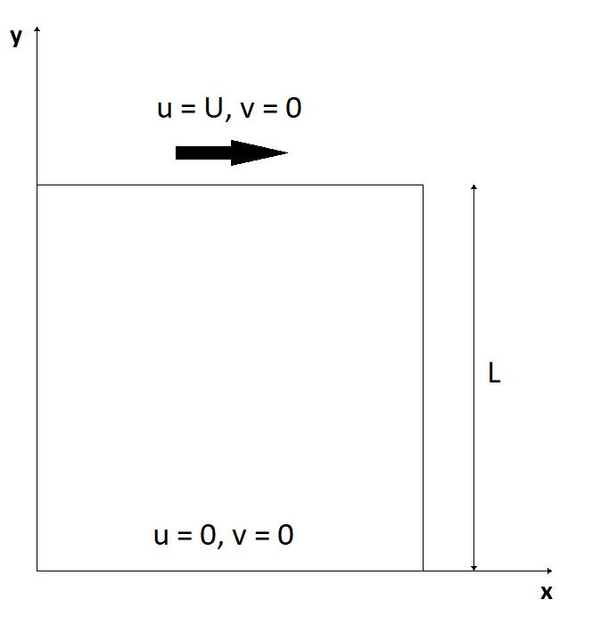
Figure 11: The Couette flow test: a schematic representation.

a no-slip (or ”wall”) boundary condition, expressed by $u=0$, is imposed in the lower plate, located at $y=0$; a non homogeneous Dirichlet’s boundary condition on the velocity, expressed by $u=U$, with $U=1$, is imposed on the upper plate; finally, periodic boundary conditions are used at the left and at the right sides of the domain. In these conditions, the steady regime that originates is a laminar flow driven by the viscous drag force. From Equations (1) and (2), if the gravity term is not considered, and since no pressure gradient is present, the only non-trivial equation remains the $x$-momentum equation:

$$-\nu\frac{\partial^{2}u}{\partial y^{2}}=0.$$ (61)

The exact solution of this problem is given by:

$$u(y)=U\frac{y}{L},$$

and, according to Newton’s law, the tangential stress is a constant given by:

$$\tau=\mu\frac{\partial u}{\partial y}=\mu\frac{U}{L}\quad\forall y\in(0,L).$$

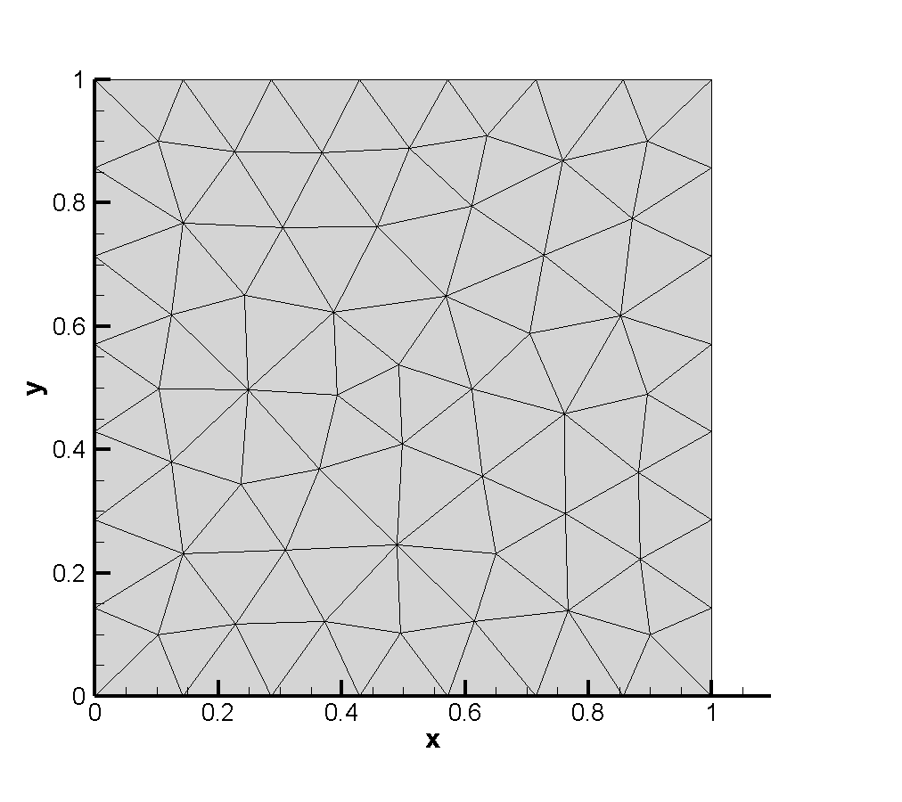
Figure 12: The unstructured mesh with $N_{e}=116$.

In order to check that our numerical method is able to reproduce the exact solution, we set up a numerical test where a coarse unstructured mesh with $N_{e}=116$ elements (Figure 12) was used and an increasing number $N$ of polynomial degrees from $0$ to $5$ was employed. The results in Table 1b confirm that the linear solution is correctly reproduced up to machine precision, for all degrees $N\geq 1$.

Table 1: Steady Couette flow test: errors in the $L^{2}$ norms for the velocity, after $20$ timesteps, obtained by $p_{\gamma}=0$ and increasing polynomial degree $N$. In column (b), the Eulerian implementation was used.

$N$	$E_{2}^{v}$
0	2.35E-02
1	8.51E-14
2	2.55E-13
3	3.05E-13
4	2.70E-13
5	2.07E-13

(a) ALE, $V=0$

$E_{2}^{v}$
2.35E-02
1.97E-14
5.82E-14
7.02E-14
2.26E-13
9.13E-12

(b) Eulerian

A comparison in terms of computational times between the new quadrature-free ALE implementation with the new discrete velocity space and the standard Eulerian approach using a simple tensor product basis on the unit square for the velocity space is reported in Figure 13. The advantage of using the new implementation is evident for the highest polynomial degree $N=5$, where we have $126$ seconds for the old and only $7$ seconds for the new implementation, which means that only $5.5\%$ of the time is required by the new scheme.

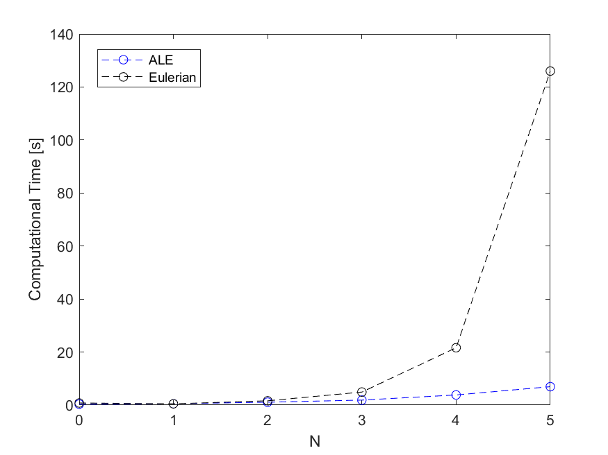
Figure 13: Steady Couette flow test: comparison between the computational times of the simulations for the ALE and the Eulerian implementations.

For the same test, also a comparison in terms of the RAM memory was carried out: the results are reported in Figure 14. We can observe that the memory required by the new algorithm is only slightly increasing with $N$ and it is significantly smaller than the old algorithm, even in a case of small number of elements, $N_{e}=116$. For example, in the simulations with $N=5$, the new algorithm required $62MB$ of RAM, versus $413MB$ of the old one, which means only $15\%$.

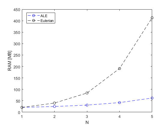
Figure 14: Steady Couette flow test: comparison between the memory usage for the ALE and the Eulerian implementations.

Now, let us study how the steady solution of the Couette flow is reached, starting from an initial condition of still fluid. Let us indicate the horizontal velocity of the fluid at height $y$ and time $t$ as $u(y,t)$. The problem is described by the parabolic equation:

$$\frac{\partial u}{\partial t}-\nu\frac{\partial^{2}u}{\partial y^{2}}=0,$$ (62)

by the boundary conditions:

$$u(0,t)=0,u(L,t)=U,\quad\forall t\in\left[0,T\right],$$

and by the initial condition:

$$u(y,0)=0,\quad\forall y\in(0,L).$$

The exact solution of this problem can be found, for example, by the method of separation of variables and is given by:

$$u(y,t)=U\frac{y}{L}-2\frac{U}{\pi}\sum_{n=1}^{\infty}\frac{1}{n}e^{-n^{2}\pi^{2}\nu\frac{t}{L^{2}}}\sin\left(n\pi\left(1-\frac{y}{L}\right)\right).$$

Also for this unsteady version of the Couette problem, we choose the following parameters: $\nu=0.01$, $L=1$, $U=1$. In Figure 15 the solution obtained by our numerical method with $N=p_{\gamma}=1$ on the coarse unstructured mesh of Figure 12 is reported, together with the plot of the exact solution, for different times ($t=0.5$, $t=1.0$, $t=5.0$, $t=10.0$). The comparison beween the numerical and the analytical solution shows a very good agreement. We observe that at large times, the solution of this problem tends towards the steady solution $u(y)=U\frac{y}{L}$ which was studied in the previous numerical test.

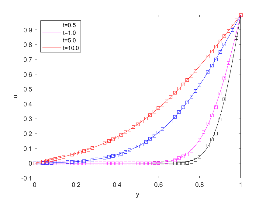
Figure 15: Unsteady Couette flow test: plots of the exact solution (continuous line) and the numerical solution (squares) at times $t=0.5$, $t=1.0$, $t=5.0$ and $t=10.0$.

In order to compare the two versions of our numerical method, we executed several simulations of the unsteady Couette flow test, up to the final time $T=10.0$. The results for a set of increasing space and time polynomial degrees $N=p_{\gamma}$ are shown in Table 2b. We can conclude, also for this numerical test, that:

1. the new ALE numerical method is consistent in the Eulerian limit, since the results obtained by the ”ALE, $V=0$” and ”Eulerian” implementations are very similar;

2. the new algorithm is cheaper from the point of view of the computational time;

3. the new algorithm is cheaper from the point of view of the computer memory usage.

Table 2: Unsteady Couette flow test: errors in the $L^{2}$ norm for the velocity, CPU computational time (in seconds), and RAM’s usage (in $MB$). In table (b), the Eulerian implementation was used.

$N=p_{\gamma}$	$E_{2}^{v}$	CPU time [$s$]	RAM [$MB$]
1	9.93E-04	46	25
2	2.67E-04	723	49
3	1.07E-04	15579	163

(a) ALE, $V=0$

$E_{2}^{v}$	CPU time [$s$]	RAM [$MB$]
8.58E-04	50	30
2.66E-04	2290	109
1.07E-04	76302	487

(b) Eulerian

5.2 The Taylor-Green vortex

As next numerical test for the incompressible Navier-Stokes equations we consider the two-dimensional version of the Taylor-Green vortex problem TaylorGreen:1937 . We consider periodic boundary conditions for the square $\Omega=[-\pi,\pi]^{2}$ and a final time given by $T=0.1$. Because of the presence of the viscous stresses, the vortices decay in time, losing energy. The analytical solution of the problem is given by:

$$u(x,y,t) = \sin(x)\cos(y)e^{-2\nu t};$$ (63)

$$v(x,y,t) = -\cos(x)\sin(y)e^{-2\nu t};$$ (64)

$$p(x,y,t) = \frac{1}{4}\left(\cos(2x)+\cos(2y)\right)e^{-4\nu t}.$$ (65)

The assessment of the order of convergence, for multiple simulations, for different polynomial degrees $N$, is reported in Table 3h and in Figure 16. We observe that the errors obtained by the two implementations are very similar, which is a confirmation of the consistency of our numerical method in the Eulerian limit. Moreover, regarding the estimated order of convergence, it is definitively close to the value $N+1$ for the $L^{2}$ norm of the velocity error, while for the pressure the value $N+1$ is clearly achieved only for the cases $N=0$ and $N=2$.

Table 3: Unsteady Taylor-Green vortex test: errors in the $L^{2}$ norms for the pressure $p$ and the velocity field $(u,v)$, and convergence ratio, obtained by $N=p_{\gamma}=0,1,2,3$ on unstructured meshes with increasing number of triangles $N_{e}$.

$N_{e}$	$E_{2}^{p}$	$E_{2}^{v}$	$\sigma_{2}^{p}$	$\sigma_{2}^{v}$
116	8.66E-01	9.66E-01	-	-
380	4.34E-01	5.48E-01	1.1	0.9
902	2.38E-01	3.64E-01	1.4	1.0
1638	1.95E-01	2.75E-01	0.6	0.9

(a) $N=0$, ALE

$N_{e}$	$E_{2}^{p}$	$E_{2}^{v}$	$\sigma_{2}^{p}$	$\sigma_{2}^{v}$
116	8.62E-01	9.65E-01	-	-
380	4.29E-01	5.48E-01	1.1	0.9
902	2.34E-01	3.64E-01	1.4	1.0
1638	1.80E-01	2.74E-01	0.8	0.9

(b) $N=0$, Eulerian

$N_{e}$	$E_{2}^{p}$	$E_{2}^{v}$	$\sigma_{2}^{p}$	$\sigma_{2}^{v}$
116	1.61E-01	1.47E-01	-	-
380	5.09E-02	4.33E-02	1.8	2.0
902	2.28E-02	1.69E-02	1.9	2.2
1638	1.69E-02	9.03E-03	0.9	1.9

(c) $N=1$, ALE

$N_{e}$	$E_{2}^{p}$	$E_{2}^{v}$	$\sigma_{2}^{p}$	$\sigma_{2}^{v}$
116	1.35E-01	1.04E-01	-	-
380	4.48E-02	3.11E-02	1.8	1.9
902	2.09E-02	1.23E-02	1.8	2.2
1638	1.18E-02	6.65E-03	1.8	1.9

(d) $N=1$, Eulerian

$N_{e}$	$E_{2}^{p}$	$E_{2}^{v}$	$\sigma_{2}^{p}$	$\sigma_{2}^{v}$
62	6.26E-02	3.95E-02	-	-
116	2.67E-02	1.69E-02	2.7	2.7
380	4.49E-03	2.52E-03	2.9	3.0
902	1.36E-03	6.50E-04	2.8	3.2

(e) $N=2$, ALE

$N_{e}$	$E_{2}^{p}$	$E_{2}^{v}$	$\sigma_{2}^{p}$	$\sigma_{2}^{v}$
62	4.40E-02	2.18E-02	-	-
116	1.87E-02	8.43E-03	2.8	3.1
380	3.57E-03	1.17E-03	2.6	3.2
902	1.11E-03	2.97E-04	2.7	3.2

(f) $N=2$, Eulerian

$N_{e}$	$E_{2}^{p}$	$E_{2}^{v}$	$\sigma_{2}^{p}$	$\sigma_{2}^{v}$
26	5.43E-02	3.30E-02	-	-
62	8.05E-03	5.48E-03	3.9	3.7
116	4.56E-03	1.47E-03	1.8	4.2
380	2.04E-03	1.08E-04	1.3	4.2

(g) $N=3$, ALE

$N_{e}$	$E_{2}^{p}$	$E_{2}^{v}$	$\sigma_{2}^{p}$	$\sigma_{2}^{v}$
26	3.63E-02	1.54E-02	-	-
62	6.54E-03	2.77E-03	3.5	3.5
116	4.64E-03	7.00E-04	1.1	4.4
380	2.06E-03	4.61E-05	1.3	4.3

(h) $N=3$, Eulerian

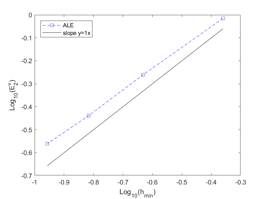
(a) $N=p_{\gamma}=0$

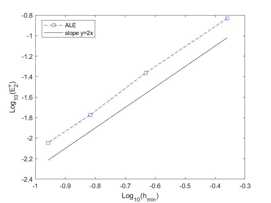
(b) $N=p_{\gamma}=1$

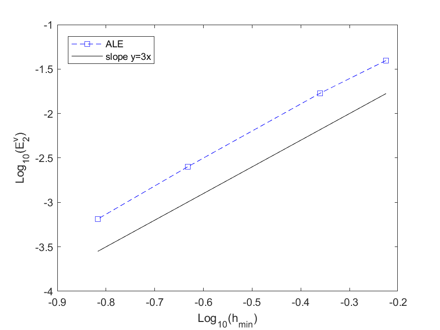
(c) $N=p_{\gamma}=2$

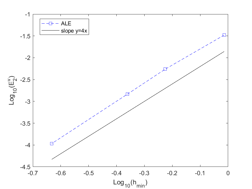
(d) $N=p_{\gamma}=3$

Figure 16: Unsteady Taylor-Green vortex test: slope in the logarithmic plane of the $L^{2}$ norm of the error for the velocity field $(u,v)$, for different polynomial degrees.

For this numerical test, the analysis of the computational times is reported in Figure 17. The new ALE algorithm requires the recomputation of all the matrices listed in Formulae (40)-(48), at every time-step of the simulation. For this reason, we expect it to be slower than the Eulerian one. Instead, for the cases $N=0,1$ and $2$, this tendency is inverted, independently from the mesh size. We can state that this is a consequence of two facts.
Firstly, in our new geometry-free implementation, the pre-computational time is reduced to almost zero, because the algorithm only needs to read an input binary file for the universal tensors which have already been computed analytically on the reference space–time elements. On the contrary, the pre-computational time of the Eulerian algorithm is dependent on the employed mesh, and it is larger for larger mesh sizes.
Secondly, the Lagrangian recalculation of the matrices is written in such a way to be very efficient from the computational point of view: the resulting matrices in (40)-(48) come from an operation of tensor-reduction between the precomputed universal tensors and the updated coefficients containing the geometric information of the mesh (see Remark 4.1). From the results of the computational times, it is evident that, up to the case $N=p_{\gamma}=2$, the first data of this multiplication are so small that they can be stored in the first levels of the memory cache, allowing a very fast recalculation of the matrices. But, for the last case, $N=p_{\gamma}=3$, the access to these larger data is not very fast anymore, because their dimension exceeds the dimension of the cache, therefore the simulations turn out to be slower.

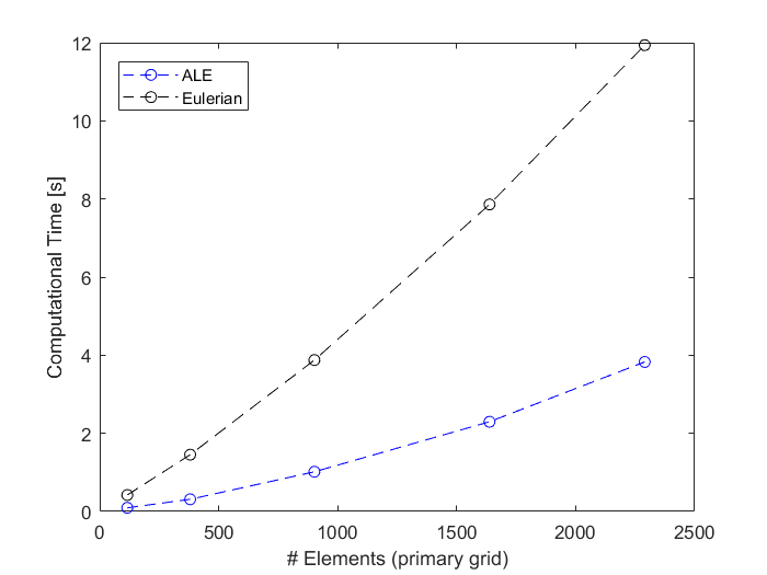
(a) $N=p_{\gamma}=0$

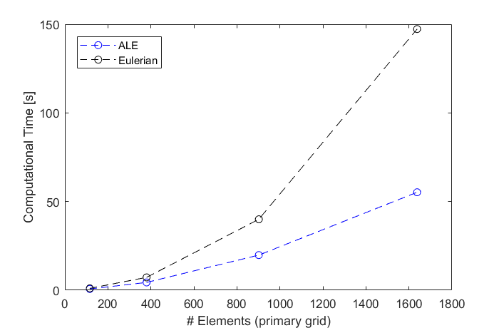
(b) $N=p_{\gamma}=1$

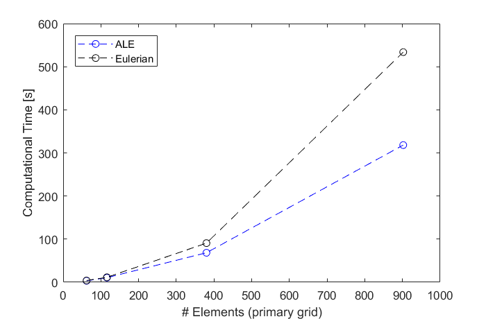
(c) $N=p_{\gamma}=2$

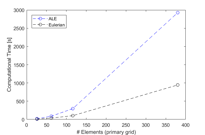
(d) $N=p_{\gamma}=3$

Figure 17: Unsteady Taylor-Green vortex test: comparison between the computational times of the simulations for the ALE and the Eulerian implementations.

Afterwards, an analysis of the required memory can be found in Table 4c. The advantage of using the new approach becomes more important, the larger is the mesh size. As it was expected, the required memory increases when increasing the parameters $N$, $p_{\gamma}$ and $N_{e}$, also for the ALE implementation. But an increase of $N_{e}$ only affects the dimension of the variables to be stored (e.g. the array for the nodes of the mesh, the arrays for the space–time degrees of freedom of the solution, …) and not the universal tensors, whose size only depends on $N$ and $p_{\gamma}$. Viceversa, in the Eulerian implementation, we must store all the local matrices (40)-(48) which occupy a very large part of the memory and which are directly proportional to the mesh size $N_{e}$. For this reason, the Eulerian implementation required a bigger amount of memory, for every numerical test that we have performed. In the tests that we have performed with the coarsest meshes, the ALE implementation required about the half of the memory of the Eulerian one.

Table 4: Unsteady Taylor-Green vortex test: memory usage (in $MB$), required by the ALE and the Eulerian implementations, and percentage of the first with respect to the second, for different polynomial degrees.

$N_{e}$	ALE, $V=0$	Eulerian	Percentage
116	25	31	80.6 %
380	39	52	75.0 %
902	65	96	67.7 %
1638	102	168	60.7 %

(a) $N=p_{\gamma}=1$

$N_{e}$	ALE, $V=0$	Eulerian	Percentage
62	49	67	73.1 %
116	67	106	63.2 %
380	179	311	57.6 %
902	392	709	55.3 %

(b) $N=p_{\gamma}=2$

$N_{e}$	ALE, $V=0$	Eulerian	Percentage
26	110	120	91.7 %
62	181	262	69.1 %
116	279	472	59.1 %
380	800	1497	53.4 %

(c) $N=p_{\gamma}=3$

5.3 The lid-driven cavity

The lid-driven cavity test, which was proposed for the first time in Ghia1982 , has become a standard benchmark for the verification of the numerical solvers of the incompressible Navier-Stokes equations. Indeed, despite its geometrical simplicity, this test has got a complex flow regime which is characterized by the formation of some interesting vortices at the corners of the cavity.
Let us consider the square domain $\Omega=[-0.5,0.5]^{2}$ and let us define the following boundary conditions (see Figure 18):

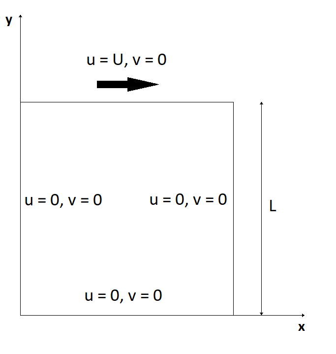
Figure 18: The lid-driven cavity flow test: a schematic representation.

• no-slip (”wall”-type) conditions at the bottom, at the left and at the right of the domain: $u=0$, $v=0$ and $\frac{\partial p}{\partial\vec{n}}=0$ (zero normal derivative of the pressure);

• Dirichlet’s boundary condition for the velocity at the top of the domain: $u=1$, $v=0$ and $\frac{\partial p}{\partial\vec{n}}=0$ (zero normal derivative of the pressure).

Let us consider an initial condition of still fluid inside the domain ($u=0$, $v=0$). The final simulation time $T$ is determined by the following tolerance criterion:

$$\max_{j=1,\ldots,N_{d}}{|\hat{\mathbf{v}}_{j}^{n+1}-\hat{\mathbf{v}}_{j}^{n}|}<\epsilon.$$ (66)

The simulation stops when the $L^{\infty}$ norm of the difference of the velocity fields from two consecutive solutions is below a tolerance value, $\epsilon=10^{-6}$. In this way, we can state that the steady solution of the problem has been reached.
For the case $Re=100$, we used a coarse unstructured mesh with $N_{e}=116$ and we got the results depicted in Figure 19a at around $T=8$, by using $N=3,p_{\gamma}=0$. Then, for the case $Re=400$, we used exactly the same discretization parameters and we obtained the results in Figure 19b at around $T=20$. Finally, we used $N=3,p_{\gamma}=0$ and an unstructured mesh with $N_{e}=902$ for the case $Re=1000$, and we obtained the results shown in Figure 19c, at around $T=25$. From these plots, it is evident that not only the primary, central vortex, but also the two smaller, counter-rotating vortices in the two lower corners of the cavity (BR₁ and BL₁, using the notation in Ghia1982 ) are well reproduced by our numerical method. We observe that, thanks to the use of the high-order in space $N=3$, the numerical solver is able to handle the singularities of the pressure and of the velocity field at the two upper corners, even if a quasi-uniform mesh with a modest number of elements is employed.

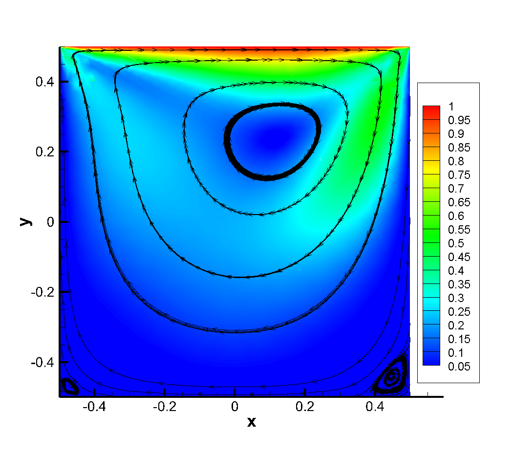
(a) $Re=100$

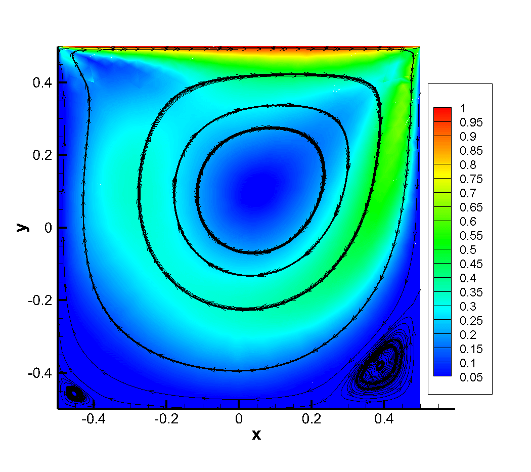
(b) $Re=400$

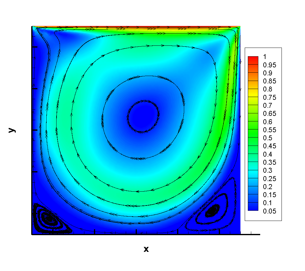
(c) $Re=1000$

Figure 19: Lid-driven cavity test: plots of the velocity’s magnitude and streamlines, at the final simulation time $T$, for different values of the Reynolds number.

In order to have a quantitative assessment of the solution, we evaluate the velocity components at the two middle lines of the cavity $x=0$ and $y=0$, and we compare them with the reference results provided in Ghia1982 . The red lines in all the graphs of Figure 20 refer to the high-order $N=3$ simulations that have been described above, showing a very good agreement with the reference data, both for the $u$ and the $v$ functions, for every case of the employed Reynolds number. In the same graphs, also the results given by the low-order method $N=1$ obtained for different meshes (the mesh size $N_{e}$ is reported in the legend of the graphs) are shown. We point out that the high-order $N=3$ scheme is very accurate because the differences with the low-order scheme applied to very refined meshes are almost indistinguishable. However, the benefits of using the high-order scheme can be clearly appreciated from the comparison of the performances with the low-order scheme (see Table 5b).

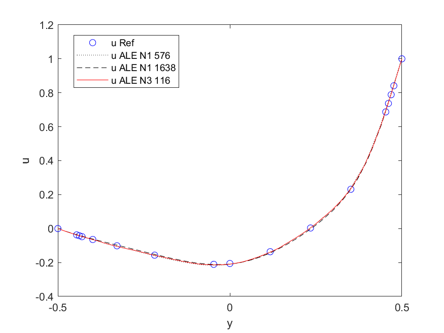
(a) $u(0.5,y,T)$, $Re=100$

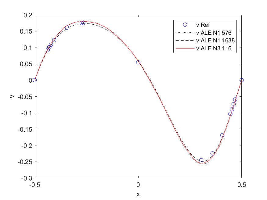
(b) $v(x,0.5,T)$, $Re=100$

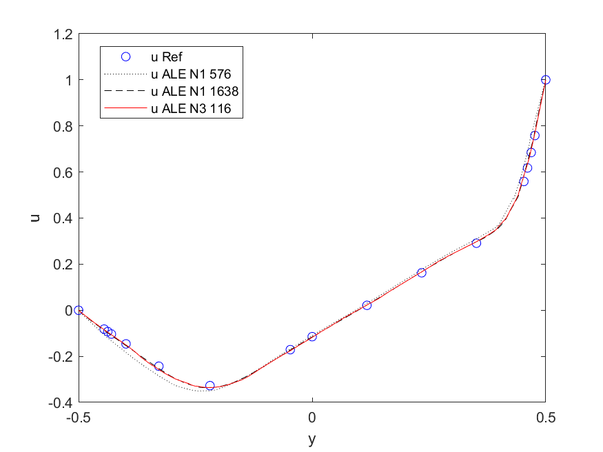
(c) $u(0.5,y,T)$, $Re=400$

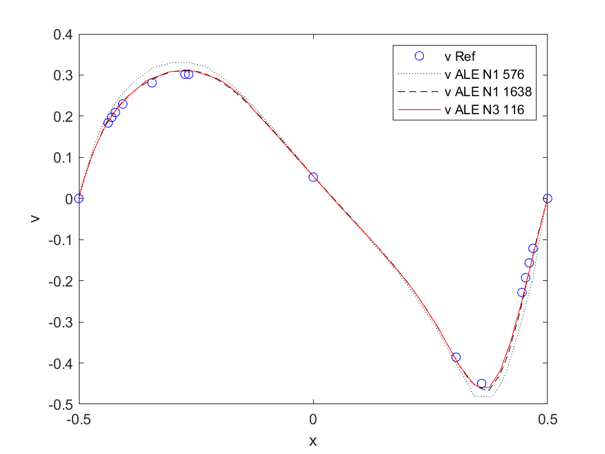
(d) $v(x,0.5,T)$, $Re=400$

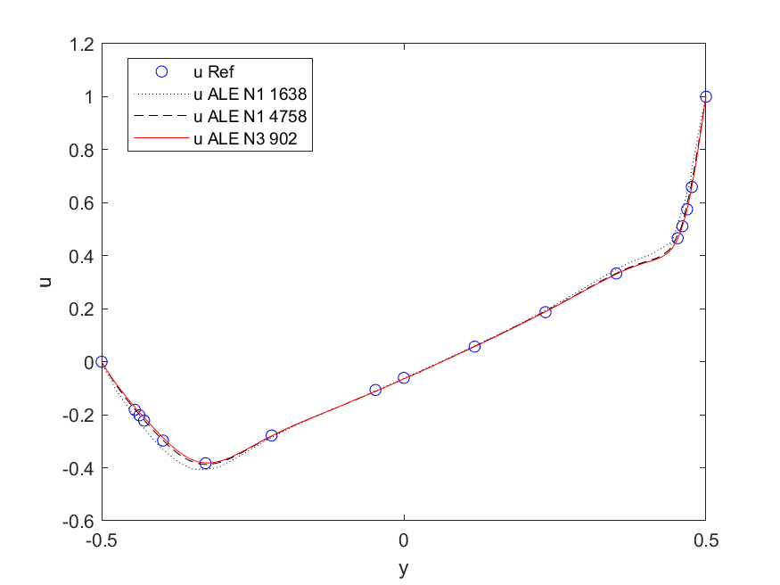
(e) $u(0.5,y,T)$, $Re=1000$

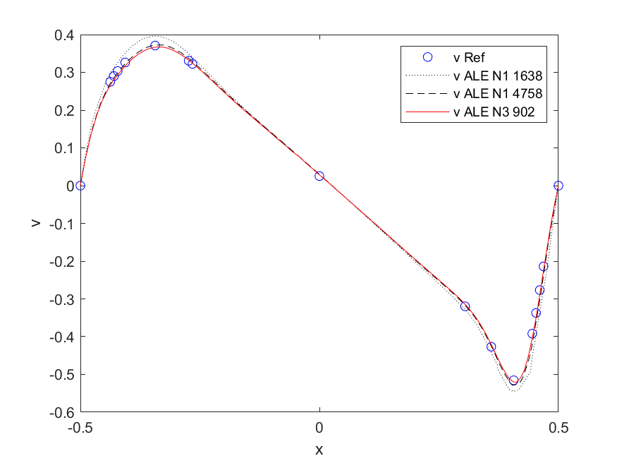
(f) $v(x,0.5,T)$, $Re=1000$

Figure 20: Lid-driven cavity test: plots of the velocity components in the middle lines of the domain, for different values of the Reynolds number.

Table 5: Lid-driven cavity test: comparison of the performances between the high-order ($N=3$) and low-order ($N=1$) schemes, in the cases $Re=400$ (a) and $Re=1000$ (b).

	ALE N$3$ $116$	ALE N$1$ $1638$	Percentage
$N_{e}$	116	1638	7.1%
CPU time [$min$]	21	111	18.9%
RAM [$MB$]	33	44	75.0%

(a) $Re=400$

	ALE N$3$ $902$	ALE N$1$ $4758$	Percentage
$N_{e}$	902	4758	19.0%
CPU time [$min$]	492	706	69.7%
RAM [$MB$]	86	112	76.8%

(b) $Re=1000$

5.4 The Blasius boundary layer

Another classical benchmark for the incompressible Navier-Stokes equations is the formation of the laminar boundary layer over a flat plate. Let us consider a steady laminar flow with velocity field $\vec{v}=(U,0)$ which passes over a flat plate with length $L$. Under the assumptions that there are no gravity forces and the pressure is constant, a self-similar solution of the Navier-Stokes equations was found by Blasius in Blasius1908 . The Blasius equations (third-order non-linear differential equations) are given by:

$$\left\{\begin{array}[]{l}f^{\prime\prime\prime}+ff^{\prime\prime}=0,\\ f(0)=0,\quad f^{\prime}(0)=0,\quad\lim_{\xi\rightarrow\infty}f^{\prime}(\xi)=1,\end{array}\right.$$ (69)

where $\xi=y\sqrt{\frac{U}{2\nu x}}$ is the Blasius coordinate and $f^{\prime}=\frac{u}{U}$.
Let us consider a square domain and let us use the following boundary conditions (see Figure 21):

• (”inflow”-type) Dirichlet’s boundary condition for the velocity on the left of the domain: $u=U$, $v=0$ and $\frac{\partial p}{\partial\vec{n}}=0$ (zero normal derivative of the pressure);

• no-slip (”wall”-type) conditions on the flat plate: $u=0$, $v=0$ and $\frac{\partial p}{\partial\vec{n}}=0$ (zero normal derivative of the pressure);

• (”outflow”-type) Dirichlet’s boundary condition for the pressure on the top and on the right of the domain and before the flat plate: $p=1$ and $\frac{\partial\vec{v}}{\partial\vec{n}}=0$ (zero normal derivative of both the velocity components).

Figure 21: Blasius boundary layer: a scheme of the boundary conditions.

As initial conditions, we impose $p=1$ and the farfield velocity field $\vec{v}=(U,0)$ inside the domain, with $U=1$. We use an unstructured mesh with $N_{e}=576$ elements and we employ a polynomial degree $N=3$ in space and $p_{\gamma}=0$ in time. We set the kinematic viscosity coefficient to $\nu=3.125\cdot 10^{-4}$ and we study the resulting boundary layer at the distances $L=0.4$ and $L=0.7$ of the flat plate, so that the local Reynolds number $Re_{L}=\frac{UL}{\nu}$ is equal to $Re_{L}=1280$ and $Re_{L}=2240$, respectively. The simulation stopped at time $T=2.7$, when a steady state was reached, according to the criterion in Formula (66), with tolerance $\epsilon=10^{-6}$. In Figure 22, the results of the numerical solution, in the $\xi-u$ plot, are compared with the reference Blasius solution obtained in DumbserNSE by a tenth-order DG Ordinary Differential Equations (ODE) solver with a classical shooting method for the boundary conditions. A very good agreement can be observed, despite the use of a quite coarse mesh. Moreover, the self-similarity property of the solution is verified.

(a) $x=0.4$

(b) $x=0.7$

Figure 22: Blasius boundary layer test: comparison between the reference solution (continuous line) and the numerical solution (squares), at distances (a) $x=0.4$ and (b) $x=0.7$ from the attachment point of the boundary layer.

6 Conclusions

In this article, we have presented a new high order accurate staggered semi-implicit space–time discontinuous Galerkin method for the two dimensional incompressible Navier-Stokes equations. The numerical scheme is based on the work proposed in STINS2D ; STINS2DTri ; STCNS , but is oriented towards the Arbitrary Lagragian Eulerian framework thanks to the use of a suitable pair of velocity-pressure finite elements. The same polynomial degree $N$ is employed for representing both the pressure and the velocity, therefore it is named an equal-order-interpolation finite element method.
The new scheme has been verified through several benchmarks in fluid dynamics, from the Couette flow to the cavity flow and the Blasius boundary layer. The numerical results agree very well to the reference solutions in all the numerical tests that we have performed. The high order of accuracy has been verified in the Taylor-Green vortex test, up to $N=3$ and $p_{\gamma}=3$.
The consistency in the Eulerian limit has been assessed by comparing the results obtained with the staggered space–time DG algorithm proposed in STINS2DTri . Compared to the Eulerian implementation, the new ALE implementation proposed here is not only computationally more efficient, but also less memory consuming, since all universal matrices are precomputed before runtime, once and for all, on a reference element. Indeed, all local matrices in the Galerkin formulation can be updated, with their geometric information, at every time-step $n$, by a cheap tensor-reduction operation.

Conflict of interest

On behalf of all authors, the corresponding author states that there is no conflict of interest.

References

- [1] F. Bassi, A. Crivellini, D.A. Di Pietro, and S. Rebay. On a robust discontinuous Galerkin technique for the solution of compressible flow. J. Comput. Phys., 218:208–221, 2006.
- [2] F. Bassi, A. Crivellini, D.A. Di Pietro, and S. Rebay. An implicit high-order discontinuous Galerkin method for steady and unsteady incompressible flows. Comput. & Fluids, 36:1529–1546, 2007.
- [3] F. Bassi and S. Rebay. A high-order accurate discontinuous finite element method for the numerical solution of the compressible Navier–Stokes equations. J. Comput. Phys., 131:267–279, 1997.
- [4] C.E. Baumann and J.T. Oden. A discontinuous hp finite element method for the Euler and Navier-Stokes equations. Int. J. Numer. Meth. Fl., 31(1):79–95, 1999.
- [5] J. B. Bell, P. Coletta, and H. M. Glaz. A second-order projection method for the incompressible Navier-Stokes equations. J. Comput. Phys., 85:257–283, 1989.
- [6] D. J. Benson. Momentum advection on a staggered mesh. J. Comput. Phys., 100(1):143 – 162, 1992.
- [7] A. Bermudez, A. Dervieux, J.A. Desideri, and M.E. Vazquez. Upwind schemes for the two–dimensional shallow water equations with variable depth using unstructured meshes. Comput. Method. Appl. M., 155:49–72, 1998.
- [8] A. Bermúdez, J.L. Ferrín, L. Saavedra, and M.E. Vázquez-Cendón. A projection hybrid finite volume/element method for low-Mach number flows. J. Comput. Phys., 271:360–378, 2014.
- [9] M. Berndt, J. Breil, S. Galera, M. Kucharik, P.H. Maire, and M. Shashkov. Two-step hybrid conservative remapping for multimaterial arbitrary Lagrangian–Eulerian methods. J. Comput. Phys., 230:6664–6687, 2011.
- [10] H. Blasius. Grenzschichten in Flüssigkeiten mit kleiner Reibung. Z. Angew. Math. Phys., 56:1–37, 1908.
- [11] P. Bochev, D. Ridzal, and M. J. Shashkov. Fast optimization-based conservative remap of scalar fields through aggregate mass transfer. J. Comput. Phys., 246:37–57, 2013.
- [12] S. Boscarino, F. Filbet, and G. Russo. High Order Semi-implicit Schemes for Time Dependent Partial Differential Equations. J. Sci. Comput., 68:975–1001, 2016.
- [13] S. Boscarino, P.G. LeFloch, and G. Russo. High-Order Asymptotic-Preserving Methods for Fully Nonlinear Relaxation Problems. SIAM J. Sci. Comput., 36:A377–A395, 2014.
- [14] S. Boscarino, G. Russo, and L. Scandurra. All Mach Number Second Order Semi-implicit Scheme for the Euler Equations of Gas Dynamics. J. Sci. Comput., 77:850–884, 2018.
- [15] W. Boscheri. An efficient high order direct ALE ADER finite volume scheme with a posteriori limiting for hydrodynamics and magnetohydrodynamics. Int. J. Numer. Meth. Fl., 134-135:111–129, 2016.
- [16] W. Boscheri, D.S. Balsara, and M. Dumbser. Lagrangian ADER-WENO finite volume schemes on unstructured triangular meshes based on genuinely multidimensional HLL riemann solvers. J. Comput. Phys., 267:112–138, 2014.
- [17] W. Boscheri and M. Dumbser. Arbitrary-Lagrangian-Eulerian one-step WENO finite volume schemes on unstructured triangular meshes. Commun. Comput. Phys., 14:1174–1206, 2013.
- [18] W. Boscheri and M. Dumbser. A direct Arbitrary-Lagrangian–Eulerian ADER-WENO finite volume scheme on unstructured tetrahedral meshes for conservative and non-conservative hyperbolic systems in 3D. J. Comput. Phys., 275:484 – 523, 2014.
- [19] W. Boscheri and M. Dumbser. An efficient quadrature-free formulation for high order arbitrary-lagrangian–eulerian ader-weno finite volume schemes on unstructured meshes. J. Sci. Comput., 66:240–274, 2016.
- [20] W. Boscheri and M. Dumbser. Arbitrary-Lagrangian-Eulerian Discontinuous Galerkin schemes with a posteriori subcell finite volume limiting on moving unstructured meshes. J. Comput. Phys., 346:449–479, 2017.
- [21] W. Boscheri, M. Dumbser, and D.S. Balsara. High-order ADER-WENO ALE schemes on unstructured triangular meshes – application of several node solvers to hydrodynamics and magnetohydrodynamics. Int. J. Numer. Meth. Fl., 76:737–778, 2014.
- [22] W. Boscheri, M. Dumbser, and O. Zanotti. High order cell-centered lagrangian-type finite volume schemes with time-accurate local time stepping on unstructured triangular meshes. J. Comput. Phys., 291:120–150, 2014.
- [23] W. Boscheri and R. Loubère. High order accurate direct Arbitrary-Lagrangian-Eulerian ADER-MOOD finite volume schemes for non-conservative hyperbolic systems with stiff source terms. Commun. Comput. Phys., 21:271–312, 2017.
- [24] W. Boscheri, R. Loubère, and M. Dumbser. Direct Arbitrary-Lagrangian–Eulerian ADER-MOOD finite volume schemes for multidimensional hyperbolic conservation laws. J. Comput. Phys., 292:56–87, 2015.
- [25] J. Breil, T. Harribey, P.H. Maire, and M.J. Shashkov. A multi-material ReALE method with MOF interface reconstruction. Comput. & Fluids, 83:115–125, 2013.
- [26] A.N. Brooks and T.J.R. Hughes. Stream-line upwind/Petrov Galerkin formulation for convection dominated flows with particular emphasis on the incompressible Navier-Stokes equation. Comput. Method. Appl. M., 32:199–259, 1982.
- [27] L. Brugnano and V. Casulli. Iterative solution of piecewise linear systems. SIAM J. Sci. Comput., 30:463–472, 2007.
- [28] L. Brugnano and V. Casulli. Iterative solution of piecewise linear systems and applications to flows in porous media. SIAM J. Sci. Comput., 31:1858–1873, 2009.
- [29] L. Brugnano and A. Sestini. Iterative solution of piecewise linear systems for the numerical solution of obstacle problems. J. Numer. Anal. Ind. Appl. Math., 6:67–82, 2012.
- [30] E.J. Caramana, D.E. Burton, M.J. Shashkov, and P.P. Whalen. The construction of compatible hydrodynamics algorithms utilizing conservation of total energy. J. Comput. Phys., 146:227–262, 1998.
- [31] G. Carré, S. Del Pino, B. Després, and E. Labourasse. A cell-centered Lagrangian hydrodynamics scheme on general unstructured meshes in arbitrary dimension. J. Comput. Phys., 228:5160–5183, 2009.
- [32] V. Casulli. A high-resolution wetting and drying algorithm for free-surface hydrodynamics. Int. J. Numer. Meth. Fl., 60:391–408, 2009.
- [33] V. Casulli. A semi-implicit numerical method for the free-surface Navier–Stokes equations. Int. J. Numer. Meth. Fl., 74:605–622, 2014.
- [34] V. Casulli and E. Cattani. Stability, accuracy and efficiency of a semi-implicit method for three-dimensional shallow water flow. Comput. Math. Appl., 27:99–112, 1994.
- [35] V. Casulli and R.T. Cheng. Semi-implicit finite difference methods for three-dimensional shallow water flow. Int. J. Numer. Meth. Fl., 15:629–648, 1992.
- [36] V. Casulli, M. Dumbser, and E. F. Toro. Semi-implicit numerical modeling of axially symmetric flows in compliant arterial systems. Int. J. Numer. Meth. Bio., 28:257–272, 2012.
- [37] V. Casulli and D. Greenspan. Pressure method for the numerical solution of transient, compressible fluid flow. Int. J. Numer. Meth. Fl., 4:1001–1012, 1984.
- [38] V. Casulli and G. S. Stelling. Semi-implicit subgrid modelling of three-dimensional free-surface flows. Int. J. Numer. Meth. Fl., 67:441–449, 2011.
- [39] V. Casulli and R.A. Walters. An unstructured grid, three-dimensional model based on the shallow water equations. Int. J. Numer. Meth. Fl., 32:331–348, 2000.
- [40] V. Casulli and P. Zanolli. Iterative solutions of mildly nonlinear systems. J. Comput. Appl. Math., 236:3937–3947, 2012.
- [41] J. Cesenek, M. Feistauer, J. Horacek, V. Kucera, and J. Prokopova. Simulation of compressible viscous flow in time-dependent domains. Appl. Math. Comput., 219:7139–7150, 2013.
- [42] A.J. Chorin. A numerical method for solving incompressible viscous flow problems. J. Comput. Phys., 2:12–26, 1967.
- [43] A.J. Chorin. Numerical solution of the Navier–Stokes equations. Math. Comput., 23:341–354, 1968.
- [44] E.T. Chung and B. Engquist. Optimal discontinuous Galerkin methods for wave propagation. SIAM J. Numer. Anal., 44:2131–2158, 2006.
- [45] E.T. Chung and C.S. Lee. A staggered discontinuous Galerkin method for the convection–diffusion equation. J. Numer. Math., 20:1–31, 2012.
- [46] B. Cockburn, S. Hou, and C.W. Shu. The Runge-Kutta local projection discontinuous Galerkin finite element method for conservation laws IV. The multidimensional case. Math. Comput., 54:545–581, 1990.
- [47] B. Cockburn, S.Y. Lin, and C.W. Shu. TVB Runge-Kutta local projection discontinuous Galerkin finite element method for conservation laws III: one dimensional systems. J. Comput. Phys., 84:90–113, 1989.
- [48] B. Cockburn and C. W. Shu. The local discontinuous Galerkin method for time-dependent convection-diffusion systems. SIAM J. Numer. Anal., 35:2440–2463, 1998.
- [49] B. Cockburn and C.W. Shu. TVB Runge-Kutta local projection discontinuous Galerkin finite element method for conservation laws II. General framework. Math. Comput., 52:411–435, 1989.
- [50] B. Cockburn and C.W. Shu. The Runge-Kutta local projection P1-discontinuous Galerkin finite element method for scalar conservation laws. ESAIM - Math. Model. Num., 25:337–361, 1991.
- [51] B. Cockburn and C.W. Shu. The Runge-Kutta discontinuous Galerkin method for conservation laws V: multidimensional systems. J. Comput. Phys., 141:199–224, 1998.
- [52] B. Cockburn and C.W. Shu. Runge–Kutta discontinuous Galerkin methods for convection-dominated problems. J. Sci. Comput., 16:173–261, 2001.
- [53] F. Cordier, P. Degond, and A. Kumbaro. An Asymptotic-Preserving all-speed scheme for the Euler and Navier-Stokes equations. J. Comput. Phys., 231:5685–5704, 2012.
- [54] A. Crivellini, V. D’Alessandro, and F. Bassi. High-order discontinuous Galerkin solutions of three-dimensional incompressible RANS equations. Comput. & Fluids, 81:122–133, 2013.
- [55] V. Dolejsi. Semi-implicit interior penalty discontinuous galerkin methods for viscous compressible flows. Commun. Comput. Phys., 4:231–274, 2008.
- [56] V. Dolejsi and M. Feistauer. A semi-implicit discontinuous galerkin finite element method for the numerical solution of inviscid compressible flow. J. Comput. Phys., 198:727–746, 2004.
- [57] V. Dolejsi, M. Feistauer, and J. Hozman. Analysis of semi-implicit dgfem for nonlinear convection-diffusion problems on nonconforming meshes. Comput. Method. Appl. M., 196:2813–2827, 2007.
- [58] L. Dubcova, M. Feistauer, J. Horacek, and P. Svacek. Numerical simulation of interaction between turbulent flow and a vibrating airfoil. Comput. Vis. Sci., 12:207–225, 2009.
- [59] M. Dumbser. Arbitrary high order PNPM schemes on unstructured meshes for the compressible Navier–Stokes equations. Comput. & Fluids, 39:60–76, 2010.
- [60] M. Dumbser. Arbitrary-Lagrangian–Eulerian ADER–WENO finite volume schemes with time-accurate local time stepping for hyperbolic conservation laws. Comput. Method. Appl. M., 280:57–83, 2014.
- [61] M. Dumbser, D. Balsara, E.F. Toro, and C.D. Munz. A unified framework for the construction of one-step finite-volume and discontinuous Galerkin schemes. J. Comput. Phys., 227:8209–8253, 2008.
- [62] M. Dumbser and V. Casulli. A staggered semi-implicit spectral discontinuous Galerkin scheme for the shallow water equations. Appl. Math. Comput., 219(15):8057–8077, 2013.
- [63] M. Dumbser and V. Casulli. A conservative, weakly nonlinear semi-implicit finite volume scheme for the compressible Navier–Stokes equations with general equation of state. Appl. Math. Comput., 272:479–497, 2016.
- [64] M. Dumbser, A. Hidalgo, M. Castro, C. Parés, and E.F. Toro. FORCE schemes on unstructured meshes II: Non–conservative hyperbolic systems. Comput. Method. Appl. M., 199:625–647, 2010.
- [65] M. Dumbser, U. Iben, and M. Ioriatti. An efficient semi-implicit finite volume method for axially symmetric compressible flows in compliant tubes. Appl. Numer. Math., 89:24–44, 2015.
- [66] M. Dumbser, A. Uuriintsetseg, and O. Zanotti. On Arbitrary-Lagrangian-Eulerian one-step WENO schemes for stiff hyperbolic balance laws. Commun. Comput. Phys., 14:301–327, 2013.
- [67] A. Ern and J.-L. Guermond. Theroy and Practice of Finite Elements. Springer-Verlag New York, 2004.
- [68] F. Fambri and M. Dumbser. Spectral semi-implicit and space–time discontinuous Galerkin methods for the incompressible Navier–Stokes equations on staggered Cartesian grids. Appl. Numer. Math., 110:41–74, 2016.
- [69] F. Fambri, M. Dumbser, and V. Casulli. An efficient semi-implicit method for three-dimensional non-hydrostatic flows in compliant arterial vessels. Int. J. Numer. Meth. Bio., 30:1170–1198, 2014.
- [70] M. Feistauer, J. Horacek, M. Ruzicka, and P. Svacek. Numerical analysis of flow-induced nonlinear vibrations of an airfoil with three degrees of freedom. Comput. & Fluids, 49:110–127, 2011.
- [71] M. Feistauer, V. Kucera, J. Prokopova, and J. Horacek. The ALE discontinuous Galerkin method for the simulatio of air flow through pulsating human vocal folds. AIP Conf. Proc., 1281:83–86, 2010.
- [72] E. Ferrer and R.H.J. Willden. A high order discontinuous Galerkin finite element solver for the incompressible Navier–Stokes equations. Comput. & Fluids, 46:224–230, 2011.
- [73] M. Fortin. Old and new finite elements for incompressible flows. Int. J. Numer. Meth. Fl., 1:347–364, 1981.
- [74] M.M. Francois, M.J. Shashkov, T.O. Masser, and E.D. Dendy. A comparative study of multimaterial Lagrangian and Eulerian methods with pressure relaxation. Comput. & Fluids, 83:126–136, 2013.
- [75] G. Gassner, F. Lörcher, and C.D. Munz. A contribution to the construction of diffusion fluxes for finite volume and discontinuous Galerkin schemes. J. Comput. Phys., 224:1049–1063, 2007.
- [76] U. Ghia, K.N. Ghia, and C.T. Shin. High-Re solutions for incompressible flow using Navier-Stokes equations and multigrid method. J. Comput. Phys., 48:387–411, 1982.
- [77] F.X. Giraldo and M. Restelli. High-order semi-implicit time-integrators for a triangular discontinuous Galerkin oceanic shallow water model. Int. J. Numer. Meth. Fl., 63:1077–1102, 2010.
- [78] F.H. Harlow and J.E. Welch. Numerical calculation of time-dependent viscous incompressible flow of fluid with a free surface. Phys. Fluids, 8:2182–2189, 1965.
- [79] R. Hartmann and P. Houston. Symmetric interior penalty DG methods for the compressible Navier-Stokes equations I: Method formulation. Int. J. Numer. Anal. Mod., 3:1–20, 2006.
- [80] R. Hartmann and P. Houston. An optimal order interior penalty discontinuous Galerkin discretization of the compressible Navier–Stokes equations. J. Comput. Phys., 227:9670–9685, 2008.
- [81] J.G. Heywood and R. Rannacher. Finite element approximation of the nonstationary Navier–Stokes problem. I. Regularity of solutions and second order error estimates for spatial discretization. SIAM J. Numer. Anal., 19:275–311, 1982.
- [82] J.G. Heywood and R. Rannacher. Finite element approximation of the nonstationary Navier–Stokes problem. III. Smoothing property and higher order error estimates for spatial discretization. SIAM J. Numer. Anal., 25:489–512, 1988.
- [83] A. Hidalgo and M. Dumbser. ADER schemes for nonlinear systems of stiff advection–diffusion–reaction equations. J. Sci. Comput., 48:173–189, 2011.
- [84] C.W. Hirt, A.A. Amsden, and J.L. Cook. An arbitrary Lagrangian-Eulerian computing method for all flow speeds. J. Comput. Phys., 14:227–253, 1974.
- [85] C.W. Hirt and B.D. Nichols. Volume of fluid (VOF) method for dynamics of free boundaries. J. Comput. Phys., 39:201–225, 1981.
- [86] T.J.R. Hughes, M. Mallet, and M. Mizukami. A new finite element formulation for computational fluid dynamics: II. Beyond SUPG. Comput. Method. Appl. M., 54:341–?355, 1986.
- [87] C. Klaij, J.J.W. Van der Vegt, and H. Van der Ven. Space–time discontinuous Galerkin method for the compressible Navier–Stokes equations. J. Comput. Phys., 217:589–611, 2006.
- [88] B. Klein, F. Kummer, and M. Oberlack. A SIMPLE based discontinuous Galerkin solver for steady incompressible flows. J. Comput. Phys., 237:235–250, 2013.
- [89] R. Klein. Semi-implicit extension of a godunov-type scheme based on low mach number asymptotics I: one-dimensional flow. J. Comput. Phys., 121:213–237, 1995.
- [90] C. Klingenberg, G. Schnucke, and Y. Xia. Arbitrary Lagrangian-Eulerian discontinuous Galerkin method for conservation laws: Analysis and application in one dimension. Math. Comput., 86(305):1203–1232, 2017.
- [91] M. Kucharik, J. Breil, S. Galera, P.H. Maire, M. Berndt, and M.J. Shashkov. Hybrid remap for multi-material ALE. Comput. & Fluids, 46:293–297, 2011.
- [92] M. Kucharik and M.J. Shashkov. One-step hybrid remapping algorithm for multi-material arbitrary Lagrangian–Eulerian methods. J. Comput. Phys., 231:2851–2864, 2012.
- [93] R. Liska, M.J. Shashkov, P. Váchal, and B. Wendroff. Synchronized flux corrected remapping for ALE methods. Comput. & Fluids, 46:312–317, 2011.
- [94] Y.J. Liu, C.W. Shu, E. Tadmor, and M. Zhang. Central discontinuous Galerkin methods on overlapping cells with a non-oscillatory hierarchical reconstruction. SIAM J. Numer. Anal., 45:2442–2467, 2007.
- [95] Y.J. Liu, C.W. Shu, E. Tadmor, and M. Zhang. L2 stability analysis of the central discontinuous Galerkin method and a comparison between the central and regular discontinuous Galerkin methods. ESAIM - Math. Model. Num., 42:593–607, 2008.
- [96] P.H. Maire, R. Abgrall, J. Breil, and J. Ovadia. A cell-centered Lagrangian scheme for two-dimensional compressible flow problems. SIAM J. Sci. Comput., 29:1781–1824, 2007.
- [97] C.D. Munz. On Godunov–type schemes for Lagrangian gas dynamics. SIAM J. Numer. Anal., 31:17–42, 1994.
- [98] C.D. Munz, S. Roller, R. Klein, and K.J. Geratz. The extension of incompressible flow solvers to the weakly compressible regime. Comput. & Fluids, 32:173–196, 2003.
- [99] J. Von Neumann and R.D. Richtmyer. A method for the numerical calculation of hydrodynamic shocks. J. Appl. Phys., 21:232–237, 1950.
- [100] N.C. Nguyen, J. Peraire, and B. Cockburn. An implicit high-order hybridizable discontinuous Galerkin method for the incompressible Navier-Stokes equations. J. Comput. Phys., 230:1147–1170, 2011.
- [101] J.H. Park and C.-D. Munz. Multiple pressure variables methods for fluid flow at all mach numbers. Int. J. Numer. Meth. Fl., 49(8):905–931, 2005.
- [102] S. Patankar. Numerical Heat Transfer and Fluid Flow. CRC Press, 2018.
- [103] S.V. Patankar and D.B. Spalding. A calculation procedure for heat, mass and momentum transfer in three-dimensional parabolic flows. Int. J. Heat Mass Tran., 15:1787–1806, 1972.
- [104] J.S. Peery and D.E. Carroll. Multi-material ALE methods in unstructured grids. Comput. Method. Appl. M., 187:591–619, 2000.
- [105] W.H. Reed and T.R. Hill. Triangular mesh methods for neutron transport equation. Technical Report LA-UR-73-479, Los Alamos Scientific Laboratory, 1973.
- [106] S. Rhebergen and B. Cockburn. A space–time hybridizable discontinuous Galerkin method for incompressible flows on deforming domains. J. Comput. Phys., 231:4185–4204, 2012.
- [107] S. Rhebergen, B. Cockburn, and J.J.W. van der Vegt. A space–time discontinuous Galerkin method for the incompressible Navier–Stokes equations. J. Comput. Phys., 233:339–358, 2013.
- [108] V.V. Rusanov. Calculation of interaction of non-steady shock waves with obstacles. J. Comput. Math. Phys. USSR, 1:267–279, 1961.
- [109] V.V. Rusanov. The calculation of the interaction of non-stationary shock waves and obstacles. USSR Comput. Math. Math. Phys., 1:304–320, 1962.
- [110] S.K. Sambasivan, M.J. Shashkov, and D.E. Burton. A finite volume cell-centered Lagrangian hydrodynamics approach for solids in general unstructured grids. Int. J. Numer. Meth. Fl., 72:770–810, 2013.
- [111] S.K. Sambasivan, M.J. Shashkov, and D.E. Burton. Exploration of new limiter schemes for stress tensors in Lagrangian and ALE hydrocodes. Comput. & Fluids, 83:98–114, 2013.
- [112] K. Shahbazi, P.F. Fischer, and C.R. Ethier. A high-order discontinuous Galerkin method for the unsteady incompressible Navier–Stokes equations. J. Comput. Phys., 222:391–407, 2007.
- [113] R.W. Smith. AUSM (ALE): a geometrically conservative arbitrary Lagrangian–Eulerian flux splitting scheme. J. Comput. Phys., 150:268–286, 1999.
- [114] A.H. Stroud. Approximate Calculation of Multiple Integrals. Prentice-Hall Inc., Englewood Cliffs, New Jersey, 1971.
- [115] M. Tavelli and M. Dumbser. A high order semi-implicit discontinuous Galerkin method for the two dimensional shallow water equations on staggered unstructured meshes. Appl. Math. Comput., 234:623–644, 2014.
- [116] M. Tavelli and M. Dumbser. A staggered semi-implicit discontinuous Galerkin method for the two dimensional incompressible Navier–Stokes equations. Appl. Math. Comput., 248:70–92, 2014.
- [117] M. Tavelli and M. Dumbser. A staggered space-time discontinuous Galerkin method for the incompressible Navier–Stokes equations on two-dimensional triangular meshes. Comput. & Fluids, 119:235–249, 2015.
- [118] M. Tavelli and M. Dumbser. A staggered space–time discontinuous Galerkin method for the three-dimensional incompressible Navier–Stokes equations on unstructured tetrahedral meshes. J. Comput. Phys., 319:294–323, 2016.
- [119] M. Tavelli and M. Dumbser. A pressure-based semi-implicit space–time discontinuous Galerkin method on staggered unstructured meshes for the solution of the compressible Navier–Stokes equations at all Mach numbers. J. Comput. Phys., 341:341–376, 2017.
- [120] M. Tavelli and M. Dumbser. Arbitrary high order accurate space–time discontinuous Galerkin finite element schemes on staggered unstructured meshes for linear elasticity. J. Comput. Phys., 366:386–414, 2018.
- [121] C. Taylor and P. Hood. A numerical solution of the Navier-Stokes equations using the finite element technique. Comput. & Fluids, 1:73–100, 1973.
- [122] G.I. Taylor and A.E. Green. Mechanism of the production of small eddies from large ones. P. Roy. Soc. A-Math. Phy., 158:499–521, 1937.
- [123] E.F. Toro, A. Hidalgo, and M. Dumbser. FORCE schemes on unstructured meshes I: Conservative hyperbolic systems. J. Comput. Phys., 228:3368–3389, 2009.
- [124] G. Tumolo, L. Bonaventura, and M. Restelli. A semi-implicit, semi-Lagrangian, p-adaptive discontinuous Galerkin method for the shallow water equations. J. Comput. Phys., 232:46–67, 2013.
- [125] J.J.W. van der Vegt and H. van der Ven. Space–time discontinuous Galerkin finite element method with dynamic grid motion for inviscid compressible flows: I. General formulation. J. Comput. Phys., 182:546–585, 2002.
- [126] H. van der Ven and J.J.W. van der Vegt. Space–time discontinuous Galerkin finite element method with dynamic grid motion for inviscid compressible flows: II. Efficient flux quadrature. Comput. Method. Appl. M., 191:4747–4780, 2002.
- [127] J. van Kan. A second-order accurate pressure correction method for viscous incompressible flow. SIAM J. Sci. Stat. Comp., 7:870–891, 1986.
- [128] R. Verfürth. Finite element approximation of incompressible Navier-Stokes equations with slip boundary condition II. Numer. Math., 59:615–636, 1991.
- [129] J. Yan and C.W. Shu. A local discontinuous Galerkin method for KdV type equations. SIAM J. Numer. Anal., 40:769–791, 2002.
- [130] Y.V. Yanilkin, E.A. Goncharov, V.Y. Kolobyanin, V.V. Sadchikov, J.R. Kamm, M.J. Shashkov, and W.J. Rider. Multi-material pressure relaxation methods for Lagrangian hydrodynamics. Comput. & Fluids, 83:137–143, 2013.