A Deep Exposure in High Resolution X-Rays Reveals the Hottest Plasma in the $\zeta\,$Puppis Wind

Abstract

We have obtained a very deep exposure ($813\,\mathrm{ks}$) of $\zeta\,$Puppis (O4 supergiant) with the Chandra HETG Spectrometer. Here we report on analysis of the $1$–$9\,\mathrm{\AA}$ region, especially well suited for Chandra, which has a significant contribution from continuum emission between well separated emission lines from high-ionization species. These data allow us to study the hottest plasma present through the continuum shape and emission line strengths. Assuming a powerlaw emission measure distribution which has a high-temperature cut-off, we find that the emission is consistent with a thermal spectrum having a maximum temperature of $12\,\mathrm{MK}$ as determined from the corresponding spectral cut-off. This implies an effective wind shock velocity of $900\,\mathrm{km\,s^{-1}}$, well below the wind terminal speed of $2250\,\mathrm{km\,s^{-1}}$. For X-ray emission which forms close to the star, the speed and X-ray flux are larger than can be easily reconciled with strictly self-excited line-deshadowing-instability models, suggesting a need for a fraction of the wind to be accelerated extremely rapidly right from the base. This is not so much a dynamical instability as a nonlinear response to changing boundary conditions.

tablenum SIXtablenum

1 Introduction

$\zeta\,$Puppis is one of the optically brightest O-stars, and is close at an estimated distance of only $332\,\mathrm{pc}$ (Howarth & van Leeuwen, 2019). As such, this O4If(n)p star (Sota et al., 2011) has been the target of many important studies to characterize its variability and properties. Much of this work was summarized in a recent analysis of optical spectroscopy and high-precision photometry by Ramiaramanantsoa et al. (2018), to whom we refer readers for relevant background discussion about the target star.

$\zeta\,$Pup’s relatively high X-ray flux of about $10^{-11}\,\mathrm{ergs\,cm^{-2}\,s^{-1}}$ ($1$–$40\,\mathrm{{\mbox{\AA}}}$) allows detailed analysis of its spectrum when dispersed by the High Energy Transmission Grating Spectrometer (HETGS) aboard the Chandra X-ray Observatory. An existing $68\,\mathrm{ks}$ Chandra/HETGS spectrum of $\zeta\,$Pup was analyzed by Cassinelli et al. (2001) who demonstrated that the spectrum is well described by multi-temperature thermal plasma models. To take advantage of the HETGS high resolution by driving down the statistical errors, we have obtained an additional 813 kiloseconds of exposure time for this star.

Below about $9\,\mathrm{{\mbox{\AA}}}$, the resolution of the HETGS and the low emission line density allows a relatively clean separation between lines and continuum. The thermal Bremsstrahlung (free-free) continuum shape is sensitive to the hottest plasmas expected ($\sim 10\,\mathrm{MK}$). In addition, the emission lines in this region are from highly ionized species (H- and He-like ions) of relatively abundant elements (Mg, Si, S, Ar, Ca, Fe), and are also formed at high temperatures.

The XMM-Newton spacecraft has been used to study this star, starting with Kahn et al. (2001) and continuing with the extensive series of papers (e.g. Nazé et al., 2012, 2018). However, the sensitivity of the RGS instrument aboard the XMM-Newton spacecraft is much lower below $9\,\mathrm{{\mbox{\AA}}}$ and its lower resolution impedes the clear separation of the continuum and emission lines. Hence, HETG is the best current instrument for study of both the line and continuum emission in the short wavelength region we concentrate on here.

In this paper, our primary interest is in determinateion of plasma temperatures, in particular the characterization and measurement of high-temperature lines and continuum in the Chandra/HETGS spectrum of $\zeta\,$Pup. If X-ray emission originates solely from embedded-wind shocks (Lucy & White, 1980; Feldmeier et al., 1995), then the maximum temperature is determined by the highest relative velocities of the colliding structures, and the amount of emission is indicative of the emitting volume. Hot thermal plasmas emit strongly in bound-bound lines of highly ionized states, in thermal Bremsstrahlung radiation, and in bound-free continuum emission. Bremsstrahlung and bound-free emission drop exponentially for photon energies larger than about $kT$ of the plasma (in which $k$ is Boltzmann’s constant and $T$ is the plasma temperature). For some plasma temperatures, bound-free emission can exceed that from thermal Bremsstrahlung at high energies (Landi, 2007; Kaastra et al., 2008). However, the continuum shape is similar to that from Bremsstrahlung. The the drop in the spectrum at high energies (short wavelengths) is sensitive to the hottest temperatures present in a multi-thermal plasma. Thermal emission lines are also very sensitive to temperature, having temperatures of peak emissivities that increase with atomic number; they typically emit most strongly over a range in temperature of about 0.3 dex (defined by the full-width-half-maximum of their emissivity curves). Hence, we concentrate here on the 2–9 Å region due to the relative sparseness of emission lines, the high temperature sensitivity, and the reduced importance of wind absorption. The temperature sensitivity occurs because for the expected plasma temperatures from embedded wind shocks ($2$–$10\,\mathrm{MK}$), the spectrum will drop accordingly somewhere in the $1$–$10\,\mathrm{{\mbox{\AA}}}$ range. In this regime, the wind absorption is relatively unimportant since the continuum opacity (due mainly to K-shell absorption by metals) drops very steeply to short wavelengths, so we do not have to be concerned with the wind density structure to interpret the spectral shape.

This new dataset allows us to probe the highest temperature plasma with unprecedented precision, providing a basic test for any models of X-ray production. Our aim is to use simple but robust methods to infer this maximum temperature.

2 Observations, Calibration, and Analysis

The observations analyzed here are part of a Cycle 19 Large Project (PI Waldron, Sequence Number 201176), to which we also added the first HETGS spectrum from 2000 (PI Cassinelli, Observation ID 640). Chandra Observations were made with the HETG in conjunction with the ACIS-S detector array, a configuration known as HETGS, the High Energy Transmission Grating Spectrometer (Canizares et al., 2005). An observing log is given in Table 1. We note that secular changes in the HETGS sensitivity have largely occurred at longer wavelengths than those we are concerned with here (less than 10% change below $5\,\mathrm{{\mbox{\AA}}}$), making it relatively easy to seamlessly include the ObsID 640 data with the more recent data. Any remaining small changes in the instrument’s properties are dealt with through calibration, as described below.

Spectra were extracted using standard CIAO procedures (version 4.11; Fruscione et al., 2006), using calibration database version 4.8.2. For each of the 22 observations, we extracted the positive and negative first diffraction-order count-spectra for the two types of gratings (High and Medium Energy Gratings, or HEG and MEG). For each of these count spectra, responses were computed from CIAO programs—the effective area files, or “ARFs”, and the response matrices, or “RMFs”. The latter encodes the energy-dependent line-spread function and enclosed count fraction for the extraction aperture used.

The variability in the $2$–$9\,\mathrm{{\mbox{\AA}}}$ spectral region is small enough to justify our analysis of the overall mean spectrum (see Section 4). Detailed analysis of the X-ray variability of this star will be described in a separate paper (Nichols, et al., in preparation).

While background is usually negligible for HETGS due to the ability to do spectral order-sorting through rejection of events using the intrinsic energy resolution of the detector, background does become appreciable in our analysis in the 1.7–3.0 Å region where the source flux and the effective area both drop (the effective area at $3\,\mathrm{{\mbox{\AA}}}$ is about $75\,\mathrm{cm^{2}}$ but is only $18\,\mathrm{cm^{2}}$ at $1.8\,\mathrm{{\mbox{\AA}}}$). The interesting high-temperature lines of Fe xxv, $\lambda 1.85\,\mathrm{{\mbox{\AA}}}$ (maximum emissivity at $\sim 60\,\mathrm{MK}$) occur in this region, along with the continuum from the highest temperature plasma. Hence, we have included background spectra, taken from regions adjacent to the dispersed spectra, in our analysis. This is always done by adding background-count to model-count spectra during fitting; the only time we subtract background counts from the data is for the purposes of visualization.

Fitting and modeling were done using the Interactive Spectral Interpretation System (ISIS, Houck & Denicola, 2000) which provides interfaces to an atomic database (“AtomDB”; Foster et al., 2012) for atomic data and emissivities used to construct plasma models (including bound-free, free-free, two-photon, and dielectronic recombination processes); it provides access to Xspec models, from which we used “phabs” for absorption, which is based on cross-sections from Verner et al. (1996). This absorptions model is adequate for the spectral region of interest since the major sources of opacity are inner-shell electrons of high $Z$ ions. The ionization state and non-Solar abundances of C, N and O do not matter below $\sim 10\,\mathrm{{\mbox{\AA}}}$. ISIS also has features which facilitate simultaneous modeling of the 88 spectra (22 observations with 4 orders each) and their associated responses.

The fundamental paradigm in X-ray spectral analysis is iterative forward folding, in which the instrumental response is applied to a model spectrum via an integral equation in order to generate model counts. A background (empirical or model) is optionally added to the model counts. The model parameters are adjusted (for fitting done here, usually with an amoeba-subplex optimization method) to minimize the residuals between the observed and model counts, using Poisson counting statistics. This is necessary because while the response matrix is nearly diagonal for diffraction grating instruments, it still has significant off-diagonal terms (representing the spectral resolution and instrumental profile), and cannot be inverted uniquely. The only robust method is to maintain each count-spectrum and their individual reponses. We do use an approximate “unfolding” for visualization in division of the counts by the model count rate per unit flux. This does not deconvolve line profiles, nor is it guaranteed to be accurate in regions of rapidly changing spectral response with wavelength. But it is good for visualization of the data in model space and for assessing the overall quality of the fit (residuals are still formed between modeled and observed counts). To improve efficiency in fitting, we combine datasets across observations and orders for each grating type; that is, we combine HEG positive and negative orders, and likewise for MEG. This means that models only need to be evaluated twice, once for each grid. Internally to the system, however, each dataset and response are still unique: model counts are evaluated for each array, then counts are summed, models are summed, and residuals computed. Hence, we can work with any subset of the 22 observations without creating actual files (counts and responses) for each permutation of interest.

Table 1: Observations Analyzed

ObsID	Observation Start Time	Exposure
		[ks]
640	2000-03-28T13:31:41	67.7
21113	2018-07-01T20:18:49	17.7
21112	2018-07-02T22:57:54	29.7
20156	2018-07-03T16:06:38	15.5
21114	2018-07-05T17:00:36	19.7
21111	2018-07-06T05:00:09	26.9
21115	2018-07-07T03:17:11	18.1
21116	2018-07-08T02:20:58	43.4
20158	2018-07-30T22:36:40	18.4
21661	2018-08-03T11:42:46	96.9
20157	2018-08-08T23:32:35	76.4
21659	2018-08-22T02:13:29	86.3
21673	2018-08-24T18:52:10	15.0
20154	2019-01-25T03:21:34	47.0
22049	2019-02-01T00:55:26	27.7
20155	2019-07-15T00:04:38	19.7
22278	2019-07-16T16:20:37	30.5
22279	2019-07-17T14:52:40	26.0
22280	2019-07-20T06:45:30	25.5
22281	2019-07-21T21:13:28	41.7
22076	2019-08-01T00:47:34	75.1
21898	2019-08-17T03:16:06	55.7

3 Spectral Modeling

We proceeded in iterative steps in modeling the spectral region below $9\,\mathrm{{\mbox{\AA}}}$. Since emission lines are present which are formed at very different temperatures (e.g, Mg xi and S xvi), the plasma is not iso-thermal, so we began by fitting a two-temperature-component model to provide overall plasma characteristics and to guide further analysis. For our more definitive multi-temperature thermal plasmas, each temperature component is constrained to have the same line shape, elemental abundances, and multiplicative absorption function. Because for the purposes of this paper we are primarily interested only in the line strengths (as a probe of temperature, abundance, and absorption), a Doppler shifted and broadened Gaussian is used to model the emission line shapes. A more detailed analysis of the lines would include distributed wind absorption and emission in an expanding medium (see, e.g. Owocki & Cohen, 2001; Oskinova et al., 2006; Zhekov & Palla, 2007), but as can be seen from the fits displayed later, this simpler model is adequate for our purposes of modeling the overall line fluxes and separating the lines from the continuum. Whatever the actual physical effects determining the line shapes, it is fortunate that the lines seem simply shifted rather than strongly asymmetric (see the fits in Cassinelli et al., 2001; Waldron & Cassinelli, 2001). Likewise, the absorption is not really a foreground screen of absorption; our assumption is similar to the “exospheric” approximation (Owocki & Cohen, 1999), which assumes all emission is from above the wind optical depth for X-ray emission, $\tau_{\lambda}=1$. This is reasonable for the shorter wavelengths which can be seen from geometrically deep in the wind, as far down as the photosphere (see Figure 5 in Oskinova et al., 2006). We add a “foreground” screen of absorption to approximate the distributed wind absorption. This should be reasonable in understanding the shape of the spectral energy distribution. In the more detailed analysis of broad-band X-ray absorption of Leutenegger et al. (2010), it was found that below $10\,\mathrm{{\mbox{\AA}}}$, the foreground absorbing screen approximation was adequate.

The free parameters per plasma temperature component are then the temperature and normalization (emission measure). The line width and shift were determined independently by fitting line-dense regions ($\sim 9$–$13\,\mathrm{{\mbox{\AA}}}$) with an AtomDB model template, and then frozen. We used a uniform Doppler shift of $-450\,\mathrm{km\,s^{-1}}$ and a Gaussian broadening term (in addition to thermal broadening) with a full-width half-maximum of about $1900\,\mathrm{km\,s^{-1}}$, which is reasonable given the terminal wind velocity of $2250\,\mathrm{km\,s^{-1}}$ (Puls et al., 2006). The apparent Doppler shift is a signature of wind absorption, due to line-of-sight absorption of the receding wind’s X-ray emission. In general, these parameters change with wavelength, due to the region of formation in the wind. Using the mid-spectrum gives us an average value, and later during fitting we bin the spectrum substantially so that we are not so sensitive to the specific values; we are primarily interested in the continuum shape and the integrated line fluxes as temperature diagnostics. We defer detailed line profile analysis to a follow-up paper (in preparation).

Abundances of Mg, Si, S, and Ar were left free; for $2T$ fits, these parameters are degenerate with $T$. The result is a provisional model which gives a reasonable match to the observed spectrum. It required temperatures of about $6.0$ and $14\,\mathrm{MK}$, with emission measures of $2.6\times 10^{55}$ and $2.3\times 10^{54}\,\mathrm{cm^{-3}}$.

The absorption term required a column of $N_{\mathrm{H}}\sim 4\times 10^{21}\,\mathrm{cm^{-2}}$. For comparison, the interstellar column is only $2\times 10^{20}\,\mathrm{cm^{-2}}$, using the color excess in the blue-to-visual color magnitudes, $E(B-V)=0.04$ (Howarth & van Leeuwen, 2019) and the standard dust-to-gas ratio scaling relation, $N_{\mathrm{H}}\approx 5\times 10^{21}\times E(B-V)\,\mathrm{cm^{-2}}$. While this spectral region is less sensitive to wind absorption than the overall X-ray spectrum, it is not negligible. Our model is not sufficient to apply to the entire HETG region, but since we are mainly interested in the highest temperature, this is well constrained (to about $0.1\,$dex). Improvements to a global model will come when line profiles are modeled in detail.

Using this provisional model, we evaluated the presence of “line-free” regions by taking the ratio of the total to the continuum-only model count spectrum, and defined line-free as regions where the deviation from the model continuum is below 5%. Over the $2$–$9\,\mathrm{{\mbox{\AA}}}$ range, about 45% of the resolution elements are line-free (at HEG or MEG resolution; the lines are resolved in each channel). Above $9\,\mathrm{{\mbox{\AA}}}$, there are no such regions. Over $2$–$9\,\mathrm{{\mbox{\AA}}}$, 20% of the photon flux is from the line-free regions, whereas the complement 80% of the region’s flux is about equally divided between line and continuum photons.

We attempted fits to just the line-free region, but the lower counts made for much more uncertain parameters. The hotter plasma continuum only becomes appreciable below about 3–4 Å, where signal drops. The lines of Mg, Si, S, Ar, Ca, and Fe are needed to constrain plasmas having temperatures from 6–60$\,\mathrm{MK}$. The lines contribute significantly to the counts improving the overall statistics, and they provide substantial leverage on temperature determination.

For a more physically motivated model than the 2-temperature fit, such as might be encountered with an ensemble of shocks in a clumpy wind (see, for example Cassinelli et al., 2008; Ignace et al., 2012), we have adopted a power-law differential emission measure ($DEM$) model of the form,

$$dEM/dT=[n_{e}n_{H}\,dV/dT]=D_{0}(r)\,T^{-\beta},$$ (1)

where $dEM/dT$ is the differential emission measure, $V$ is the volume of X-ray-emitting plasma, $D_{0}$ is a normalization factor, $n_{e}$ and $n_{H}$ are the electron and hydrogen number densities, respectively, $T$ is the plasma temperature which we limit to a range $T_{\mathrm{min}}$, $T_{\mathrm{max}}$, and the exponent $\beta$. In Appendix A we derive an analytic solution for the continuum spectral energy distribution in the limit of $T_{\mathrm{min}}=0$ (also see Brown, 1974).

We have implemented a power-law $DEM$ in ISIS using a weighted sum of AtomDB model spectra on an evenly spaced logarithmic temperature grid with parameters $T_{\mathrm{min}}$, $T_{\mathrm{max}}$, the $DEM$ exponent $\beta$, an overall normalization term (proportional to the volume emission measure, but not identical to $D_{0}$ in Equation 1 because the stellar distance is also included), the plasma model parameters shared by all components (Gaussian broadening, Doppler shift, and abundances), with multiplicative absorption.

Our free parameters are the normalization, $\beta$, ${T_{\mathrm{min}}}$, ${T_{\mathrm{max}}}$, ${N_{\mathrm{H}}}$, and abundances of the most significant species in the region, Mg, Si, S, and Ar. We have obtained fits with these free parameters, but the statistic’s minimum is somewhat complicated with degenerate or poorly constrained parameters—better minima are often found when additional searches are performed, such as for confidence limits on parameters. Hence, we use a Markov-Chain, Monte-Carlo method (an ISIS implementation of the Foreman-Mackey et al., 2013, Python code) to search parameter space and form confidence contours. From these runs, we could easily see a strong degeneracy between the normalization and the minimum temperature. Since the minimum temperature is not an interesting parameter (and is set to zero in the theoretical derivation in Appendix A), we froze ${T_{\mathrm{min}}}$ to the best fit value of $6.0\,$dex K; it was always nearly a factor of 10 or more below ${T_{\mathrm{max}}}$. Furthermore, the shape of the spectrum, which is the primary diagnostic of the highest temperature plasma, is not very sensitive to ${T_{\mathrm{min}}}$. The fits then produced closed confidence contours for the normalization, and did not change other confidence limits. This does introduce an overall systematic uncertainty in the model, but not one which affects our primary results.

Figure 1 shows the data, model, and residuals. We only fit the spectrum below $9\,\mathrm{{\mbox{\AA}}}$, and in a few near-continuum bins near $13\,\mathrm{{\mbox{\AA}}}$ which are important for constraining $N_{\mathrm{H}}$. We also ignored the Si xiii intercombination and forbidden lines near $6.7\,\mathrm{{\mbox{\AA}}}$, since these are strongly affected by the photospheric UV radiation field, as can be seen in the residuals when we evaluate the model over this region. (In our model, we also set the Fe relative abundance to $0.5$, since this gave a better extrapolation of our fit to the $10$–$12\,\mathrm{{\mbox{\AA}}}$ region, but it is otherwise not important to the spectral region fit.)

Figure 2 shows parameter-pair confidence contours for the normalization, maximum temperature, absorbing column, and differential emission measure exponent. The relative abundance parameter pair confidence contours are shown in Figure 3. The reference abundances relevant to the region fit are listed in Table 2.

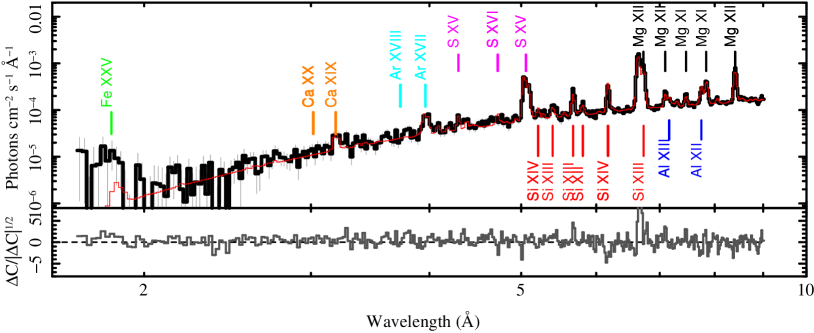
Figure 1: X-ray spectrum (black) and absorbed powerlaw emission measure distribution’ spectral model (thin red line). The figure shows the combined HEG and MEG data for the entire $881\,\mathrm{ks}$ exposure. Background has been subtracted from the data and model counts for plotting purposes. Counts have been converted to approximate flux through division by the count rate per unit flux. The lower panel shows the statistical residuals of data counts to model counts. The large residuals in the region fit are from Si xiii ($6.7\,\mathrm{{\mbox{\AA}}}$) because we have not compensated for photoexcitation which suppresses the forbidden lines and enhances the intercombination lines (the forbidden-to-intercombination line ratios for helium-like ions will continue to be very interesting for this star, but their precise strengths are not important for the global fitting being performed here). Positions of some lines have been marked (whether detected or not), using different colors for each element.

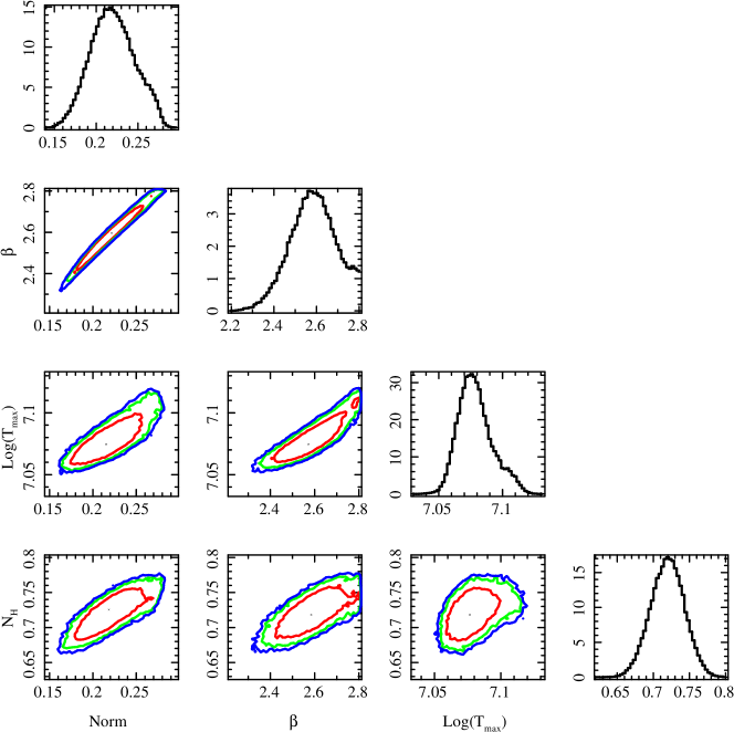
Figure 2: Parameter-pair confidence contours from 68% (inner, red), 90% (middle, green), and 95% (blue, outer). The $Norm$ is in units of $10^{-14}/(4\pi d^{2})\times VEM$ (the volume emission measure), $\beta$ is the $DEM$ exponent, temperatures are in ($\log$) K, and $N_{\mathrm{H}}$ is in units of $10^{22}\,\mathrm{cm^{-2}}$. The marginal histograms for each parameter are shown on the diagonal.

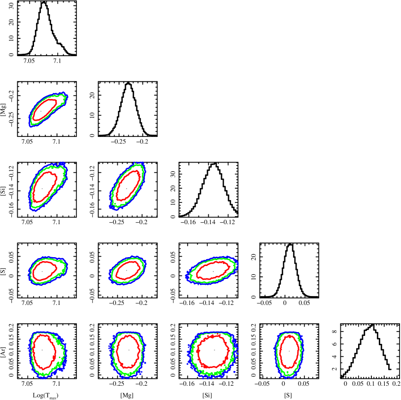
Figure 3: The abundance parameter-pair confidence contours. Abundances are given in the logarithmic difference from the values in Table 2. The marginal histograms for each parameter are shown on the diagonal.

Table 2: Reference Abundances

$Z$	Elem.	$\log N$	Mass Frac.
		(dex)
$1$	H	$12.00$	$5.98\text{\times}{10}^{-01}$
$2$	He	$11.21$	$3.85\text{\times}{10}^{-01}$
$6$	C	$7.60$	$2.85\text{\times}{10}^{-04}$
$7$	N	$9.10$	$1.05\text{\times}{10}^{-02}$
$8$	O	$8.14$	$1.30\text{\times}{10}^{-03}$
$10$	Ne	$8.02$	$1.25\text{\times}{10}^{-03}$
$12$	Mg	$7.68$	$7.06\text{\times}{10}^{-04}$
$13$	Al	$6.54$	$5.55\text{\times}{10}^{-05}$
$14$	Si	$7.60$	$6.63\text{\times}{10}^{-04}$
$16$	S	$7.21$	$3.08\text{\times}{10}^{-04}$
$18$	Ar	$6.49$	$7.32\text{\times}{10}^{-05}$
$20$	Ca	$6.43$	$6.40\text{\times}{10}^{-05}$
$26$	Fe	$7.59$	$1.29\text{\times}{10}^{-03}$

Note. — Abundances for H, He, C, N, and O are from Bouret et al. (2012), and the remainder are from the Solar mass-fraction values of Asplund et al. (2009).

4 X-Ray Variability of the Overall Flux Below 9 Å

In fitting the cumulative spectrum, we have assumed that the mean flux is representative of the typical flux, and that we don’t have large temporal variability in the spectrum. To assess global variability, we take our powerlaw emission measure model which gives a reasonable empirical match to the mean spectrum (as shown in Figure 1) and we fit only the normalization for each individual observation; we use the model spectrum and the calibration to remove any instrumental effects which might be present in a simple count-rate analysis. Tracking changes in the normalization over time will give us a first order assessment of variability. It is within the realm of possibility that the spectral shape changes without changing the normalization, but that would require enough special circumstances to render it unlikely. Figure 4 shows the model normalizations as a function of the start times of the individual observations. While there are deviations from the mean of $0.226$, the maximum fluctuations are about 12%, while most points are within one standard deviation (0.011) of the mean as expected for a constant source. While the very first HETGS spectrum of $\zeta\,$Pup from 2000 has the lowest flux, its spectral distribution is essentially identical to the recent epoch, so we chose to include it in the analysis; it contributes about $9\%$ of the counts below $10\,\mathrm{{\mbox{\AA}}}$. Hence, we believe fitting the cumulative spectrum is meaningful.

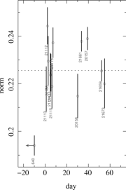
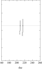
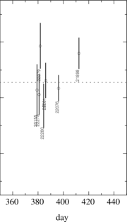
Figure 4: Normalization of a plasma model vs. time in days since the first observation in 2018. ObsID 640 has been shifted from epoch 2001 by about 6660 days. We have assumed a constant spectral shape and have fit only the normalization. Errorbars indicate 90% confidence limits. The horizontal dashed line shows the mean normalization. (The normalization is proportional to the emission measure divided by distance squared.)

5 Discussion and Conclusions

The highest temperature is a diagnostic of the maximum relative velocity of the plasma undergoing strong shocks (see, for example Feldmeier et al., 1997; Stevens et al., 1992; Cassinelli et al., 2008; Ignace et al., 2012). The maximum plasma temperature best fit for $\zeta\,$Pup is $7.08\pm 0.03\,$dex MK (or $1.04\,\mathrm{keV}$) (90% confidence). Using the relation for a strong shock, $kT=\frac{3}{16}\mu m_{\mathrm{H}}v^{2}$, where $T$ is the post-shock temperature and $v$ is the pre-shock velocity, and with the mean molecular weight $\mu=0.67$ for the adopted abundances of highly ionized elements (mainly H- and He-like ions), and using the approximation for the number of stripped electrons from Rutherford et al. (2013, Appendix C.7) , we find a maximum relative shock velocity $v\approx 900\,\mathrm{km\,s^{-1}}$ (with a formal statistical error of $\sim 50\,\mathrm{km\,s^{-1}}$ based on the temperature uncertainty). As this velocity well below the wind terminal speed, it is within the capabilities of radiative acceleration to achieve, and would be slow for a wind-wind collision in a binary. For wind expansion with a “beta-law” exponent $0.9$ (see, for example Eversberg et al., 1998), a wind speed of $900\,\mathrm{km\,s^{-1}}$ occurs at about 1.5 stellar radii above the photosphere and accelerates to about $1200\,\mathrm{km\,s^{-1}}$ by 2 stellar radii. The line-based analysis of Cohen et al. (2010) found that X-rays shortward of $10\,\mathrm{{\mbox{\AA}}}$ first appear at a turn-on radius consistent with $1.5$ stellar radii. Their results are consistent with our finding that the absorption is relatively low shortward of $10\,\mathrm{{\mbox{\AA}}}$, so any absence of emission below $1.5$ stellar radii could not be due to absorption effects. However, it has not been shown that an absence of emission at low radii is necessary to fit the X-ray emission line profiles, and additional evidence that X-ray creation may extend much deeper will be addressed in a separate publication.

The presence of a stand-off distance for the initiation of X-ray creation could be taken as evidence of line-deshadowing-instability (LDI) activity, as it is a self-excited instability that could take some distance to appear. The absence of a stand-off distance would suggest instead that variations in the acceleration right from the surface are the crucial cause. Both of these effects are considered in Sundqvist & Owocki (2013) where they find that surface perturbations are essential for generating strong shocks at low radii, and our analysis is consistent with early appearance of strong shocks, although a more in-depth analysis is required. If surface-related effects are the crucial element, then the main explanatory factor for the hard X-ray heating must trace back to the cause of variations at the boundary. Such variations could be inherent in the line-driving critical point conditions (Sundqvist & Owocki, 2015) or might require a specific physical mechanism such as subsurface convection (Cantiello et al., 2009; Cantiello & Braithwaite, 2011).

Our spectral fits led to a differential emission measure exponent of $2.6$ ($\pm 0.2$ 90% confidence). The AtomDB continuum is not purely Bremsstrahlung, but also contains radiative recombination edges and other contributions, so has additional features not included in the analytic solution. However, if we evaluate the AtomDB’s true continuum for our differential emission measure plasma model and compare to Equation A6 using Table 3, we find an exponent near $5/2$. Comparison of the spectrum to a simple powerlaw energy distribution also shows us that the curvature is significant, appearing below $5\,\mathrm{{\mbox{\AA}}}$, and that we have indeed detected the high-temperature cutoff. Our best fit is in very good agreement with the value of $7/3$ which the hydrodyamical calculations of Cassinelli et al. (2008) predicted for a bow-shock around a single clump. The models shown by Krtička et al. (2009) have a powerlaw index of about $2.4$ (see their Equation10), which is also consistent with our fitted slope. We note that their results also required enforcing some type of surface variations.

The best fit value of ${N_{\mathrm{H}}}$ of about $0.7\times 10^{22}\,\mathrm{cm^{-2}}$ seems fairly large, and also causes a spectral model extrapolation to longer wavelengths to lie well below the data beyond about $17\,\mathrm{{\mbox{\AA}}}$. However, we do not expect a constant ${N_{\mathrm{H}}}$ to apply to the entire range in our approximation, since at longer wavelengths, the optical depth is larger, and one cannot see as geometrically deeply into the wind. Furthermore, the phabs model is not valid (for stellar wind absorption modeling) at longer wavelengths because it does not incorporate warm absorbers which have edges at different wavelengths than neutral species. Below $9\,\mathrm{{\mbox{\AA}}}$, in our range of interest, the equivalent optical depths rapidly drop below unity (Oskinova et al., 2006), and we maintain our assumption that the intrinsic continuum properties dominate in the model; the standard phabs model is accurate here in determining the spectral curvature. The value of ${N_{\mathrm{H}}}$ we derived is consistent with the Fe xvii, $15\,\mathrm{{\mbox{\AA}}}$ line profile fitting of Cohen et al. (2010), who found that the optical depth on the central ray ($\tau_{*}$) was about $2.0$, and this is equivalent to ${N_{\mathrm{H}}}\sim 0.5\times 10^{22}\,\,\mathrm{cm^{-2}}$.

The shock heating rate was studied by Zhekov & Palla (2007), and by Cohen et al. (2014a) who placed upper limits on the heating rate above $T\sim 10\,\mathrm{MK}$, based on emission lines alone. We do firmly detect the high temperature lines of Ar xvii and Ca xix, whose maximum emissivities occur near $20\,\mathrm{MK}$ and $30\,\mathrm{MK}$, respectively (7.3 and 7.5 dex). However, our spectral fits do not require plasmas this hot, so their emission comes from the low-temperature tail of their emissivity curves; at $10\,\mathrm{MK}$, Ar xvii is at about 25% of its maximum emissivity, while Ca xix is at about 10%. Non-detection of both Ar xviii and Ca xx is consistent with this upper temperature limit.

There is a suggestion in the data of excess counts from Fe xxv ($1.85\,\mathrm{{\mbox{\AA}}}$), whereas the model’s line emission here is quite weak. According to the model and the atomic database, the features in the model are due to a blend of many weak Fe xxiii and Fe xxiv lines, whose emissivities peak near $32\,\mathrm{MK}$. The He-like Fe xxv emission lines peak near $63\,\mathrm{MK}$ and at $32\,\mathrm{MK}$ are still about 8 times stronger than the Fe xxiii–Fe xxiv blends. However, at the $\sim 10\,\mathrm{MK}$ maximum model temperature, Fe xxiii and Fe xxiv are only at $1\%$ of their peak emissivity, while Fe xxv is nearly an order of magnitude fainter than that. We do not think there is any significantly detected signal in Fe xxv.

Instrumental background also begins to dominate below $\sim 2\,\mathrm{{\mbox{\AA}}}$, as can be seen in the large errorbars in Figure 1; the upturn is due to amplification of the background noise. The lack of significant Fe emission and the continuum below $\sim 3\,\mathrm{{\mbox{\AA}}}$ provide good constraints on the shape of the spectrum and support the powerlaw emission measure fit here.

Abundance determinations rely on the line-to-continuum flux ratio, the theoretical emissivities, and the emission measure distribution, assuming collisional ionization equilibrium in an optically thin plasma. Mass-loss rates derived from emission lines are proportional to the adopted abundances, since they scale with the opacity (see, for examples Oskinova et al., 2006; Cohen et al., 2014b). We have assumed the emission line fluxes are only affected by foreground absorption, which is not rigorously true, since both the absorption and emission occur in the wind. We know that lines are subject to continuum absorption with Doppler effects from the wind, since line centroids are blueward of their rest wavelengths, and the red wings are affected by continuum absorption. These effects are mitigated, however, at the shorter wavelengths where the continuum opacity is smaller.

We adopted our reference abundance set for the nuclear-processed elements from Bouret et al. (2012), and the remainder as Solar from Asplund et al. (2009). We give the mass fraction and logarithmic number fractions in Table 2. We allowed the abundance parameters to range from half the reference to 1.5 times the reference values. Our results are shown in Figure 3 and show near-reference values for S and Ar, and slightly lower values for Mg and Si. They generally agree with the values found by Zhekov & Palla (2007) (but with significantly smaller uncertainties). Refinement of abundances will require more detailed line-based analysis and consideration of systematic effects due to assumed temperature distributions.

This deep Chandra/HETG spectrum of $\zeta\,$Pup has allowed us to rigorously determine that there is little to no plasma above $\sim 12\,\mathrm{MK}$ for a powerlaw differential emission measure model, and that the emission measure distribution is consistent with that expected from shocked clumps deep in the wind. Assuming efficient X-ray creation (though see Steinberg & Metzger, 2018), this limits its relative pre-shock velocities to about $900\,\mathrm{km\,s^{-1}}$. This is below the wind velocity in the acceleration zone, but is still difficult to reconcile with traditional LDI without some perturbations which can then be amplified by LDI. The hydrodynamical calculations of Sander et al. (2017) further exacerbate this: they found that the $\zeta\,$Pup wind acceleration cannot be described by a simple beta-law, but accelerates much more slowly, reaching only $0.1\times v_{\infty}$ ($\approx 200\,\mathrm{km\,s^{-1}}$) by 1.5 stellar radii above the photosphere. The inferred inefficient radiative acceleration deep in the wind presents additional challenges to understanding strong shocks within the purview of pure radiative acceleration, so additional physical mechanisms may be required. In addition, the $2D$ and $3D$ simulations of Steinberg & Metzger (2018) also present tension with our high temperature at small radii conclusion. Their simulations find that post-shock temperatures can be one or two orders of magnitude below the usual strong-shock prediction in the case of highly radiative shocks, though it is unclear how severe this restriction would be for much more weakly radiative shocks. Hence, there is clear motivation for additional theoretical and observational work to understand and reconcile these apparent differences.

Additional constraints will come from detailed line-profile modeling using radial wind structural and dynamic models; such will provide a better idea of the effective absorbing column and region of X-ray formation. The assumed foreground absorbing screen with a single value for ${N_{\mathrm{H}}}$ is an approximation; line profile fitting using detailed wind structure models will help with the interpretation of the spectral shape, especially at longer wavelengths, and also lead to important quantities such as the mass loss rate. At the short wavelengths of primary interest here, the absorption is mainly affecting the normalization and spectral curvature, but not the high energy cutoff — we are largely decoupled from the details of wind structure. Hence, we are confident that the maximum temperature is of the order we have found, and this will constrain plasma properties in future models.

Appendix A Multi-Temperature Bremsstrahlung Continuum with Temperature Cut-Off

Consider an emission measure distribution that is a power law in temperature as given by

$$\frac{dEM}{dT}=\frac{n^{2}(r)}{T_{0}}\,\left(\frac{T}{T_{0}}\right)^{-\beta}\,dV,$$ (A1)

where $EM$ is the emission measure, $T$ is temperature, $n(r)$ is the number density of the X-ray emitting plasma at radius $r$, $T_{0}$ is a temperature constant at that radius, $\beta$ is the power-law exponent at that radius and $dV$ is the volume element for a shell. In what follows, both $T_{0}$ and $\beta$ are taken as constants for all radii.

The cooling function from bremsstrahlung is given by

$$\Lambda(E,T)=\Lambda_{0}\,\left(\frac{T_{0}}{T}\right)^{1/2}\,e^{-E/kT},$$ (A2)

where $\Lambda_{0}$ is a constant. Note that there are several processes that can contribute to the emissivity in the X-ray band. At the short wavelengths of interest for this application, two-photon emission is negligible. Bound-free emission can be important across the X-ray band. However, for a wind that is predominantly H and He, such as $\zeta\,$Pup, and given relatively high temperature plasmas that contribute to the short wavelengths, Landi (2007) showed that Bremsstrahlung is most important below around $10\,\mathrm{{\mbox{\AA}}}$. Even when bound-free has a non-negligible contribution, as long as edges are not important in the waveband of interest, the cooling has the same scaling as Bremsstrahlung. In this scenario, bound-free would only impact the proportionality constant, whereas our focus is on slope information from the observed continuum. With these caveats, the following shows how the observed continuum relates to a high temperature cut-off combined with a power-law differential emission measure.

The spectral energy distribution (SED) for the continuum is $dL/dE$:

$$\frac{dL}{dE} = \int\,\Lambda(E,T)\,\frac{dEM}{dT}\,dT,$$

$$= \Lambda_{0}\,\int\,\left(\frac{T_{0}}{T}\right)^{1/2}\,e^{-E/kT}\,\frac{n^{2}(r)}{T_{0}}\,\left(\frac{T}{T_{0}}\right)^{-\beta}\,dT\,dV$$

$$= \frac{L_{0}}{kT_{0}}\,\int\,\left(\frac{T_{0}}{T}\right)^{1/2}\,e^{-E/kT}\,\left(\frac{T}{T_{0}}\right)^{-\beta}\,\frac{dT}{T_{0}},$$

where in the final line, the integration over volume has been carried out and a constant with units of luminosity, $L_{0}$ was introduced. For the present we assume that wind absorption can be ignored.

If the temperature ranges from zero to infinity, then formally, the integration above will produce a SED with $dL/dE\propto E^{-\beta+1/2}$. A high temperature cut-off leads to a downturn of the continuum towards higher energies. We now assume that the constant $T_{0}$ represents the maximum temperature achieved in every shell of the wind. The integration limits are zero to $T_{0}$. It is convenient to introduce a change of variable for normalized energy, with dummy variable $t=E/kT$ and normalized energy $x=E/kT_{0}$. The integral now becomes

$$\frac{dL}{dE}=\frac{L_{0}}{kT_{0}}\,x^{-\beta+1/2}\,\int_{x}^{\infty}\,t^{\beta-3/2}\,e^{-t}\,dt.$$ (A4)

It is convenient to introduce

$$m=\beta-3/2,$$ (A5)

in which case the specific luminosity becomes

$$\frac{dL}{dE}=\frac{L_{0}}{kT_{0}}\,x^{-m-1}\,\gamma_{\rm m}(x),$$ (A6)

where

$$\gamma_{\rm m}(x)=\int_{x}^{\infty}\,t^{\beta-3/2}\,e^{-t}\,dt.$$ (A7)

Physically, $x^{-m-1}$ is the power-law SED when there is no maximum temperature cut-off; it is $\gamma_{\rm m}(x)$ that eventually leads to an exponential decline in the SED at high energies. This integral has an analytic solution when $m$ is a non-negative integer, given by

$$\gamma_{\rm m}(x)=\left[x^{m}+mx^{m-1}+m(m-1)x^{m-2}+...+m!\right]\,e^{-x}.$$ (A8)

Here the exponential decline in normalized energy is made explicit. Table 3 provides values of $\beta$ and solutions of $\gamma_{\rm m}$ for $m=0,1,2,$ and 3.

Note that the energy flux spectrum is proportional to $dL/dE$; the photon flux spectrum is proportional to $E^{-1}\,dL/dE\propto x^{-m-2}\gamma_{\rm m}(x)$.

Table 3: Solutions of $\gamma_{\rm m}$ for Select Values of $m$

$m$	$\beta$	$\gamma_{m}(x)$
0	3/2	$e^{-x}$
1	5/2	$(x+1)\,e^{-x}$
2	7/2	$(x^{2}+2x+2)\,e^{-x}$
3	9/2	$(x^{3}+3x^{2}+6x+6)\,e^{-x}$

References

- Asplund et al. (2009) Asplund, M., Grevesse, N., Sauval, A. J., & Scott, P. 2009, ARA&A, 47, 481
- Bouret et al. (2012) Bouret, J.-C., Hillier, D. J., Lanz, T., & Fullerton, A. W. 2012, A&A, 544, A67
- Brown (1974) Brown, J. C. 1974, in IAU Symposium, Vol. 57, Coronal Disturbances, ed. G. A. Newkirk, 395
- Canizares et al. (2005) Canizares, C. R., Davis, J. E., Dewey, D., et al. 2005, PASP, 117, 1144
- Cantiello & Braithwaite (2011) Cantiello, M., & Braithwaite, J. 2011, A&A, 534, A140
- Cantiello et al. (2009) Cantiello, M., Langer, N., Brott, I., et al. 2009, A&A, 499, 279
- Cassinelli et al. (2008) Cassinelli, J. P., Ignace, R., Waldron, W. L., et al. 2008, ApJ, 683, 1052
- Cassinelli et al. (2001) Cassinelli, J. P., Miller, N. A., Waldron, W. L., MacFarlane, J. J., & Cohen, D. H. 2001, ApJ, 554, L55
- Cohen et al. (2010) Cohen, D. H., Leutenegger, M. A., Wollman, E. E., et al. 2010, MNRAS, 405, 2391
- Cohen et al. (2014a) Cohen, D. H., Li, Z., Gayley, K. G., et al. 2014a, MNRAS, 444, 3729
- Cohen et al. (2014b) Cohen, D. H., Wollman, E. E., Leutenegger, M. A., et al. 2014b, MNRAS, 439, 908
- Eversberg et al. (1998) Eversberg, T., Lépine, S., & Moffat, A. F. J. 1998, ApJ, 494, 799
- Feldmeier et al. (1997) Feldmeier, A., Puls, J., & Pauldrach, A. W. A. 1997, A&A, 322, 878
- Feldmeier et al. (1995) Feldmeier, A., Puls, J., Reile, C., et al. 1995, Ap&SS, 233, 293
- Foreman-Mackey et al. (2013) Foreman-Mackey, D., Hogg, D. W., Lang, D., & Goodman, J. 2013, PASP, 125, 306
- Foster et al. (2012) Foster, A. R., Ji, L., Smith, R. K., & Brickhouse, N. S. 2012, ApJ, 756, 128
- Fruscione et al. (2006) Fruscione, A., McDowell, J. C., Allen, G. E., et al. 2006, in Presented at the Society of Photo-Optical Instrumentation Engineers (SPIE) Conference, Vol. 6270, SPIE Conference Series
- Houck & Denicola (2000) Houck, J. C., & Denicola, L. A. 2000, in Astronomical Society of the Pacific Conference Series, Vol. 216, Astronomical Data Analysis Software and Systems IX, ed. N. Manset, C. Veillet, & D. Crabtree, 591–+
- Howarth & van Leeuwen (2019) Howarth, I. D., & van Leeuwen, F. 2019, MNRAS, 484, 5350
- Ignace et al. (2012) Ignace, R., Waldron, W. L., Cassinelli, J. P., & Burke, A. E. 2012, ApJ, 750, 40
- Kaastra et al. (2008) Kaastra, J. S., Paerels, F. B. S., Durret, F., Schindler, S., & Richter, P. 2008, Space Sci. Rev., 134, 155
- Kahn et al. (2001) Kahn, S. M., Leutenegger, M. A., Cottam, J., et al. 2001, A&A, 365, L312
- Krtička et al. (2009) Krtička, J., Feldmeier, A., Oskinova, L. M., Kubát, J., & Hamann, W. R. 2009, A&A, 508, 841
- Landi (2007) Landi, E. 2007, A&A, 476, 675
- Leutenegger et al. (2010) Leutenegger, M. A., Cohen, D. H., Zsargó, J., et al. 2010, ApJ, 719, 1767
- Lucy & White (1980) Lucy, L. B., & White, R. L. 1980, ApJ, 241, 300
- Nazé et al. (2012) Nazé, Y., Flores, C. A., & Rauw, G. 2012, A&A, 538, A22
- Nazé et al. (2018) Nazé, Y., Ramiaramanantsoa, T., Stevens, I. R., Howarth, I. D., & Moffat, A. F. J. 2018, A&A, 609, A81
- Oskinova et al. (2006) Oskinova, L. M., Feldmeier, A., & Hamann, W. 2006, MNRAS, 372, 313
- Owocki & Cohen (1999) Owocki, S. P., & Cohen, D. H. 1999, ApJ, 520, 833
- Owocki & Cohen (2001) —. 2001, ApJ, 559, 1108
- Puls et al. (2006) Puls, J., Markova, N., Scuderi, S., et al. 2006, A&A, 454, 625
- Ramiaramanantsoa et al. (2018) Ramiaramanantsoa, T., Moffat, A. F. J., Harmon, R., et al. 2018, MNRAS, 473, 5532
- Rutherford et al. (2013) Rutherford, J., Dewey, D., Figueroa-Feliciano, E., et al. 2013, ApJ, 769, 64
- Sander et al. (2017) Sander, A. A. C., Hamann, W. R., Todt, H., Hainich, R., & Shenar, T. 2017, A&A, 603, A86
- Sota et al. (2011) Sota, A., Maíz Apellániz, J., Walborn, N. R., et al. 2011, ApJS, 193, 24
- Steinberg & Metzger (2018) Steinberg, E., & Metzger, B. D. 2018, MNRAS, 479, 687
- Stevens et al. (1992) Stevens, I. R., Blondin, J. M., & Pollock, A. M. T. 1992, ApJ, 386, 265
- Sundqvist & Owocki (2013) Sundqvist, J. O., & Owocki, S. P. 2013, MNRAS, 428, 1837
- Sundqvist & Owocki (2015) —. 2015, MNRAS, 453, 3428
- Verner et al. (1996) Verner, D. A., Ferland, G. J., Korista, K. T., & Yakovlev, D. G. 1996, ApJ, 465, 487
- Waldron & Cassinelli (2001) Waldron, W. L., & Cassinelli, J. P. 2001, ApJ, 548, L45
- Zhekov & Palla (2007) Zhekov, S. A., & Palla, F. 2007, MNRAS, 382, 1124