How to Improve AI Tools (by Adding in SE Knowledge):
Experiments with the TimeLIME Defect Reduction Tool

Abstract.

AI algorithms are being used with increased frequency in SE research and practice. Such algorithms are usually commissioned and certified using data from outside the SE domain. Can we assume that such algorithms can be used “off-the-shelf” (i.e. with no modifications)? To say that another way, are there special features of SE problems that suggest a different and better way to use AI tools?

To answer these questions, this paper reports experiments with TimeLIME, a variant of the LIME explanation algorithm from KDD’16. LIME can offer recommendations on how to change static code attributes in order to reduce the number of defects in the next software release. That version of LIME used an internal weighting tool to decide what attributes to include/exclude in those recommendations. TimeLIME improves on that weighting scheme using the following SE knowledge: software comes in releases; an implausible change to software is something that has never been changed in prior releases; so it is better to use plausible changes, i.e. changes with some precedent in the prior releases. By restricting recommendations to just the frequently changed attributes, TimeLIME can produce (a) dramatically better explanations of what causes defects and (b) much better recommendations on how to fix buggy code.

Apart from these specific results about defect reduction and TimeLIME, the more general point of this paper is that our community should be more careful about using off-the-shelf AI tools, without first applying SE knowledge. As shown here, it may not be a complex matter to apply that knowledge. Further, once that SE knowledge is applied, this can result in dramatically better systems.

1. Introduction

This paper finds and fixes a flaw in a widely cited AI explanation generation method, LIME (first presented at KDD’16). In theory, LIME can be used to find code changes that make software less buggy in the next release. In practice, when we tried doing that, we found that the classic LIME model was generating surprising and unprecedented recommendations. Specifically, classic LIME kept suggesting changes that had never been seen before in the history of the project.

When we first observed this, our initial response was quite favorable. Perhaps, we thought, LIME would offer novel and powerful suggestions that would lead to greater defect reductions than ever seen before. However, as shown in this paper, classic LIME’s recommendations are sub-optimal. This paper presents TimeLIME which is a version of LIME that restricts its explanations to the attributes that change the most. On experimentation, TimeLIME’s explanations were seen to be:

• Smaller : TimeLIME restricts itself to the $M=5$ most changed attributes. Classic LIME, on the other hand, uses dozens more attributes.

• Easier to apply: The fewer the recommendations, the quicker it is to act on those recommendations.

• Better explanations: The recommendations from TimeLIME are associated with a much larger reduction in defects than classic LIME.

While TimeLIME is certainly a useful tool for proposing code changes, we argue that this is less important than how this result was generated. AI algorithms are being used with increased frequency in SE research and in SE industrial practice. If these AI tools are used “off-the-shelf” (i.e. with no modifications), then that assumes that the problems used to commission and certify these AI algorithms are relevant to SE problems. The results of this paper suggest that such assumption can be very dubious. As shown below, the performance of standard AI tools can be enhanced dramatically just by applying some SE knowledge. Specifically, the contribution of this paper is to improve classic LIME via three items of SE knowledge:

• Software comes in releases.

• An implausible change to software is something that has never been changed in prior releases.

• It is better to use plausible changes, i.e. changes with some precedence in the prior releases.

Metric	Name	Description
amc	average method complexity	Number of JAVA byte codes
avg_cc	average McCabe Average	McCabe’s cyclomatic complexity seen in class
ca	afferent couplings	How many other classes use the specific class.
cam	cohesion amongst classes	Summation of number of different types of method parameters in every method divided by a multiplication of number of different method parameter types in whole class and number of methods.
cbm	coupling between methods	Total number of new/redefined methods to which all the inherited methods are coupled
cbo	coupling between objects	Increased when the methods of one class access services of another.
ce	efferent couplings	How many other classes is used by the specific class.
dam	data access	Ratio of private (protected) attributes to total attributes
dit	depth of inheritance tree	It’s defined as the maximum length from the node to the root of the tree
ic	inheritance coupling	Number of parent classes to which a given class is coupled (includes counts of methods and variables inherited)
lcom	lack of cohesion in methods	Number of pairs of methods that do not share a reference to an instance variable.
locm3	another lack of cohesion measure	If $m$, $a$ are the number of methods, attributes in a class number and $\mu(a)$ is the number of methods accessing an attribute, then lcom3 = $((\frac{1}{a}\sum_{j}^{a}{\mu(a_{j})})-m)/(1-m)$
loc	lines of code	Total lines of code in this file or package.
max_cc	Maximum McCabe	Maximum McCabe’s cyclomatic complexity seen in class
mfa	functional abstraction	Number of methods inherited by a class plus number of methods accessible by member methods of the class
moa	aggregation	Count of the number of data declarations (class fields) whose types are user defined classes
noc	number of children	Number of direct descendants (subclasses) for each class
npm	number of public methods	Npm metric simply counts all the methods in a class that are declared as public.
rfc	response for a class	Number of methods invoked in response to a message to the object.
wmc	weighted methods per class	A class with more member functions than its peers is considered to be more complex and therefore more error prone
defect	defect	Boolean: where defects found in post-release bug-tracking systems.

Table 1. The C-K OO metrics used in defect prediction. The last variable ”defect” is the dependent variable.

Based on the experience of this paper, we caution that our community should be more careful about using off-the-shelf AI tools, without first tuning them with SE knowledge. As shown here, it is may not be a complex matter to apply that knowledge. Further, once that SE knowledge is applied, this can result in dramatically better systems.

This paper is structured around the following research questions.

RQ1: Are all explanations precedented?

We view this first result as a potential flaw in classic-LIME. As shown by RQ3, better explanations can be found using precedented explanations.

RQ2: Do developers prefer precedented explanations?

RQ3: Are precedented explanations better at defect reduction?

The rest of this paper is structured as follows. §2 discusses defect prediction and trends in the explanation literature. §3 shows our method for ranking different planning methods. §4 describes experiment and the datasets, predictive model, and planners used in this work. §5 reports our result. The credibility and reliability of our conclusions is discussed by §6. Finally, we offer conclusions and discuss future work in §7and §8.

1.1. Data Availability

All the data and scripts used in this paper are freely available online at http://github.com/anonymous12138/FSE2020.

2. Background and Related Work

2.1. Defect Prediction

The case study of this paper comes from defect prediction and planning. This kind of analysis is discussed in this section.

During software development, the testing process often has some resource limitations. For example, the effort associated with coordinated human effort across a large code base can grow exponentially with the scale of the project (Fu et al., 2016).

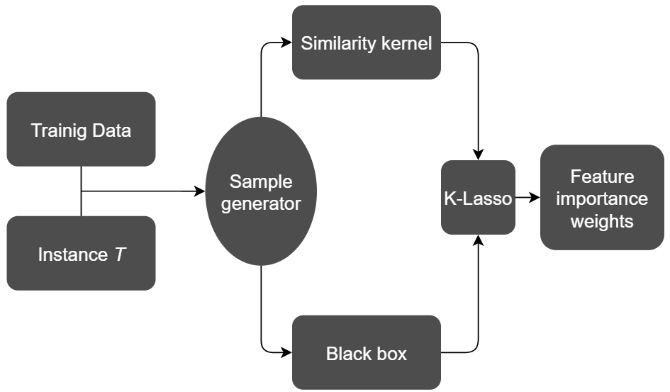
   • LIME is designed to be an add-on to other AI systems (e.g., neural network, support vector machine, and so on). Hence, it treats those AI tools as a “black box” that is queried within its processing. • Within LIME, some sample generator is used to generate synthetic data which later gets passed to the black box and a similarity kernel, along with the original training data. • The similarity kernel is an instrument used to weight the prediction results of training data returned by the black box by how similar they are to the instance T. • The K-Lasso is the procedure that learns the importance weights from the $K$ features selected with Lasso using a class of linear models.   

Figure 1. Inside LIME. From (Ribeiro et al., 2016). The feature importance weights are passed to Algorithm 1 and 2, as later elaborated in §4.3. For a sample of the output feature importance weights, see Figure 2.

Hence, to effectively manage resources, it is common to match the quality assurance (QA) effort to the perceived criticality and bugginess of the code. Since every decision is associated with a human and resource cost to the developer team, it is impractical and inefficient to distribute equal effort to every component in a software system(Briand et al., 1993). Learning defect prediction (using data miners) from static code attributes (like those shown in Table 1) is one very cheap way to “peek” at the code and decide where to spend more QA effort.

Recent results show that software defect predictors are also competitive widely-used automatic methods. Rahman et al.  (Rahman et al., 2014) compared (a) static code analysis tools FindBugs, Jlint, and PMD with (b) defect predictors (which they called “statistical defect prediction”) built using logistic regression. No significant differences in cost-effectiveness were observed. Given this equivalence, it is significant to note that defect prediction can be quickly adapted to new languages by building lightweight parsers to extract code metrics. The same is not true for static code analyzers - these need extensive modification before they can be used in new languages. Because of this ease of use, and its applicability to many programming languages, defect prediction has been extended many ways including:

1. Application of defect prediction methods to locating code with security vulnerabilities (Shin and Williams, 2013).

2. Understanding the factors that lead to a greater likelihood of defects such as defect prone software components using code metrics (e.g., ratio comment to code, cyclomatic complexity) (Menzies et al., 2010; Menzies et al., 2007) or process metrics (e.g., recent activity).

3. Predicting the location of defects so that appropriate resources may be allocated (e.g., (Bird et al., 2009))

4. Using predictors to proactively fix defects (Arcuri and Briand, 2011)

5. Studying defect prediction not only just release-level (Chen et al., 2018) but also change-level or just-in-time (Rosen et al., 2015).

6. Exploring “transfer learning” where predictors from one project are applied to another (Krishna and Menzies, 2018; Nam et al., 2018).

7. Assessing different learning methods for building predictors (Ghotra et al., [n.d.]). This has led to the development of hyper-parameter optimization and better data harvesting tools (Agrawal et al., 2018; Agrawal and Menzies, 2018a).

This paper extends defect prediction and planning in yet another way: exploring the trade-offs between explanation and planning and the performance of defect prediction models. But beyond the specific scope of this paper, there is nothing in theory stopping the application of this paper to all of the seven areas listed above (and this would be a fruitful area for future research).

2.2. Planning as Explanation Generation

In principle, once it is known how a conclusion is reached, we can query that method to find out how to change something in order to reach better conclusions. This intuition is the core of explanation-based planners. Such planning can proceed as follows:

1. Use standard means to build models that make predictions;

2. Perform what-if queries across those models to find plans on how to change the prediction.

Depending on the nature of the model, those what-if queries can be very slow (e.g., Monte Carlo simulations over a neural net model) or very fast (e.g., just use the attributes with the largest $\beta$ coefficients found by linear regression). The LIME method described later in this paper is an example of a very fast method.

2.3. Explaining “Explanations”

In our experience, software developers prefer a transparent decision-making model in which some valid rationale is provided behind each decision so that they may argue the merits of such decisions. From the perspective of transparency, the term ”explanation” or ”interpretability” refers to the extent of the human comprehension of a given AI system or the decisions made by it.

As documented in their 2019 literature review, Mueller et.al. (Mueller et al., 2019) observes that research on formal and computational models of explanation is truly vast and dates back many centuries. Formal explorations of the concept of explanation can be found in the “fourth-figure” of Aristotle (Leake, 1991). Written in the 19th century, explanation was characterized by Charles Sanders Peirce as follows: ”The surprising event C is observed. But if A were true, C would be a matter of course. Here, there is reason to suspect that A is true” (AAAI, 1990). Mueller et al. acknowledge Peirce’s historical leadership in this field but warn that Peirce’s formalism misses at least two important features: specifically, problem formulation and problem resolution. They comment that mapping an explanation back to action is “is where the hard work of explanation occurs, and that the (Peirce) model is not specific about what is involved in these steps.”

In the 1980s and 1990s, a further nuance was introduced in the the concept of explanation. Researchers exploring knowledge-based systems found that it was not enough to view explanations as a pretty print of a trace of some inference procedure. Even when the inference trace was across very succinct domain-specific languages, researchers like Leake and Clancey were surprised to see that different users wanted different kinds of explanations (Leake, 1991; Clancey, 1994). They concluded that explanation is a separate problem-solving task to inference. In their view, explanation is a procedure that customizes what to be reported according to the task at hand. Explanations, in this modern view, is context-specific: and ”the context of the current situation can significantly affect the purpose and therefore the content of an explanation” (Menzies et al., 2002).

Explanation research stresses the need for some form of plausibility operator in order to prevent the presentation of bogus explanations (Menzies et al., 2002). Consider two explanations for ”the grass is wet”. This might have happened because either because (a) it rained last night or (b) the lawn sprinkler has been left on. Hence, explaining ”wet grass” using ”rain” is a possible, but not necessarily a certain, inference. Plausibility operators (Menzies et al., 2002). can be used to assess and cull weaker explanations. Returning to the grass example, if this was a lawn in Albuquerque (which is a desert city) and if the time was high summer (which is usually very dry) then a plausibility operator would favor explanations that use “sprinkler” over “rain” since the latter is unlikely in a desert city in summertime.

It is insightful to review the LIME explanation algorithm in the context of the above paragraphs:

• In terms of mapping explanation to action, LIME takes the view that a “good” explanation is one that can change the class of some test instance. To that end, LIME builds a linear approximation model from examples near the test instance. Using that model, LIME learns what needs to be changed within the test instance in order to change the class variable of that instance (see Figure 1). The output of LIME is hence a set of attribute ranges, sorted by how much those ranges could alter a class label (see Figure 2).

• In keeping with the work from the 80s and 90s, LIME is a context-specific explanation system. Unlike data miners (that generate one model to be applied to all test instances), LIME generates a different explanation for each specific test instance.

• As to the plausibility operator, LIME uses its its own internal weighting scheme to rank explanations. The argument of this paper is that, when generating explanations over multiple consecutive releases of some software system, a useful plausibility operator is to restrict explanations to those changes seen in recent historical record of the project.

Figure 2. An example of output generated by Figure 1 when applied to the data sets of the form of Table 1. The y-axis shows the feature name and the confidence interval during which the explanation stays effective. The x-axis indicates the importance weight of each attribute. The prediction label of this instance is 1 (defective), and the weights show how each feature contributes to the prediction. A positive weight means the feature encourages the classifier to predict the instance as a positive label (1), and vice versa. Larger weights indicate greater feature importance in terms of the prediction value based on that feature weighted by a similarity kernel.

2.4. Alternatives to LIME

As mentioned above, Mueller et.al. (Mueller et al., 2019) report that the literature on explanation is truly vast. Consequently, there are many alternatives to LIME including the abductive framework of Menzies et al. (Menzies et al., 2002) or ANCHORS (Ribeiro et al., 2018) (which is another explanation algorithm generated by the same team that created LIME). Given that explanation is such a large field, it is appropriate to ask why this paper commits to the LIME view of explanation and not some other approach.

Firstly, LIME is operational whereas much of the (say) philosophical literature on explanation is insightful, but not executable.

Secondly, LIME handles an important detail that other approaches ignore. As mentioned above by Mueller et.al., some discussions on explanation ignore how to formulate problems and how to use the explanations to resolve problems. LIME, on the other hand, formulates the problem as a data mining task where “explanation” is operationalized as a regression problem learning gradients around a point in instance space. LIME also offers the following resolution operator: find attribute ranges that change the class of an instance into something more desirable.

Thirdly, LIME scales to large problems. Much recent work has results in methods to scale data mining to very large data sets. Since LIME is based on data mining, then LIME can use those scalability results in order to generate explanations for very large problems.

Fourthly, and this is more of a low-level systems reason, alternatives to LIME such as ANCHORS assume discrete classes. Our data has continuous classes which could be binarized into two discrete classes– but only at the cost of losing the information about local gradients. Hence, at least for now, we explore LIME (and will explore ANCHORS in future work).

Lastly, LIME is a widely-cited algorithm. At the time of this writing, LIME has received over 2,600 citations since it was published in 2016. Hence, methods used to improve LIME could also be useful for a wide range of other research tasks. This paper proposes precedence plausibility as a way to improve LIME.

2.5. Precedence-based Plausibility

A workshop on ”Actionable Analytics” at ASE’15(Hihn and Menzies, 2015) reported complaints from business users about the analytic models such as ”rather than apply a black-box data mining algorithm, they preferred an approach with a seemingly intuitive appeal”. Since software engineers are the target audience of explanations in SE, it is crucial to ensure the explanations are valued by them. Chen et al. say the term ”actionable” can be defined as a combination of ”comprehensible” and ”operational”(Chen et al., 2018). But how to assess ”operational”?

In this paper we make the following assumption about “operational”: a proposed change to the code is plausible if it has occurred before. That is, in this work, we claim a plan is the most operational when it has the most precedence in the history log of the project. Using this assumption, we can generate operational analytics by:

• Looking at two releases of a project and report the attributes that have changed between them;

• Next, when generating explanations, we only used those attributes that have the most changes.

After conducting a survey on 92 controlled experiments published in 12 major software engineering journals, Kampenes et al. (Kampenes et al., 2007) argues that in SE, size change can be measured via Hedge’s $g$ value(Rosenthal et al., 1994):

(1) $$g=(M_{1}-M_{2})/(S_{pooled})$$

Here, $M_{1}$ and $M_{2}$ are the means of an attribute in two consecutive releases and $S_{pooled}$ comes from 2. This expression is the pooled and weighted standard deviation ($n$ and $s$ denote the sample size and the standard deviation respectively).

(2) $$S_{pooled}=\sqrt{((n_{1}-1)s_{1}^{2}+(n_{2}-1)s_{2}^{2})/(n_{1}+n_{2}-2)}$$

3. Measuring Effectiveness: the $K$-test

This paper claims that recommendations based on TimeLIME (that focus on attributes with a history of most change) outperform recommendations generated from classical LIME. To defend that claim, we need some way to assess different planning systems.

Krishna’s $K$-test(Krishna and Menzies, 2017) uses historical data from multiple software releases to compare the effectiveness of different plans $P_{1},P_{2},....$. The test is a kind of simulation study that assumes developers were told about a plan at some prior time. After that, the test checks what happens for code that was changed in accordance (or in defiance) of that plan.

Since the test is a historical study, it requires consecutive releases $x,y,z$ of some software system. These releases are required to contain named regions of code $C_{1},C_{2},$etc that can be found in releases $x,y,z$. For example, $C_{i}$ could be an object-oriented class or a function or a file that is found in all releases. The $K$-test then assumes that there exists a quality measure $Q$ that reports the value of the regions of named code in different releases. In this study, we will use NDPV (Number of Defects in Previous Version) as the quality measure, which is described later in §4.4. Some method is then applied that uses $Q$ to reflect on the releases $x,y$ in order to infer a plan $P_{i}$ for improving release $z$.

Given the above, the $K$-test collects four quantities:

1. $G_{x,y}$: the list of Hedge’s $g$ scores for each feature in release $x,y$

2. $\Delta_{y,z}$: the delta between code $C_{i}$ in releases $y,z$.

3. $J_{y,z}=\Delta_{y,z}\cap P_{i}$: the overlap between the proposed plan and the code changes;

4. $Q_{z}-Q_{y}$: i.e. the change in the quality of the named code regions between release $y,z$.

The $K$-test assumes that “good” plans have the following property:

$$(Q_{z}-Q_{y})\propto|J_{y,z}|$$

That is, increasing the size of the overlap between the proposed plan and the observed changes is associated with an increase in the quality of release $z$. That is to say, the $K$-test defines better plans as follows:

DEFINITION: Plan $P_{i}$ is “better” that plan $P_{j}$ if, in release $z$, $P_{i}$ is associated with most quality improvements.

For our purposes, the $K$-test procedure in this paper consists of four steps:

• Train some black-box classifier on version $x$.

• Use the classifier and training data to build the explainer in LIME.

• Use the classifier and explainer to generate plans with the aim of fixing bugs reported in version $y$. Note that, in this step, TimeLIME will combine the explanations from the explainer and the historical data analysis to generate plans.

• On the same set of files that are reported buggy in version $y$, we measure the overlap score of each plan and the changes in the version $z$ using the Jaccard similarity function. Meanwhile, we also record the change in the number of bugs between the version $y$ and version $z$.

For each instance, we compare the extent of overlap between the recommended plan $P_{i}$ generated by the planner and the actual developer action in the next release as $\Delta_{y,z}$ using the Jaccard similarity coefficient.

(3) $$J_{y,z}(P_{i},\Delta_{y,z})=(P_{i}\cap\Delta_{y,z})/(P_{i}\cup\Delta_{y,z})$$

Then we convert the coefficient into percentage as our overlap score. As an example shown in Figure 3, the overlap score is

$$3/4\times 100\%=75\%$$

Formally speaking, the $K$-test is not a deterministic statement that some plan will necessarily improve quality is some future release of a project. Such deterministic causality is a precisely defined concept with the property that a single counterexample can refute the causal claim (AAAI, 1990). The $K$-test does not make such statements.

Instead, the $K$-test is a statement of historical observation. Plans that are “better” (as defined above) are those which, in the historical log, have been associated with increased values on some quality measure. Hence, they have some likelihood (but no certainty) that they will do so for future projects.

Table 3. A toy example of how to compute the overlap score using Jaccard similarity function in Eq. (3). Plans P that match the developer actions are marked gray.

	AMC	LOC	LCOM	CBO
Current release y	0.2	0.1	0.9	0.5
$P_{i}$ from release z	[0.1, 0.3]	[0, 0.1]	[0.2, 0.5]	[0.7, 0.9]
Next release z	0.2	0.3	0.3	0.7
Match?	y	n	y	y

4. Experimental Methods

The experiment reports the performance of the classical LIME and TimeLIME by comparing the quality of plans recommended by each method.

Firstly, we use an over-sampling tool called SMOTE(Chawla et al., 2002) to transform the imbalanced datasets in which defective instances may only take a small ratio of the population. This was needed since, in many of the prior papers that explored our data, researchers warn that small target classes made it harder to build predictors (Agrawal and Menzies, 2018b).

Secondly, as discussed above, we train the predictor $P$ and explainer $E$ on data of version $x$. Then in version $y$ we use the explainer to generate explanations only on those data that are reported as buggy. We also use the predictor $P$ to determine whether we should provide recommendation plans to the instance.

Then we measure the overlap score of our recommended plan and the actual change on the same file in version $z$. To do this, only select instances that are defective and whose file name has appeared in all releases of data to be instances in need of recommendations.

The above steps are used for classical LIME as well as the TimeLIME planner proposed by this paper. In the classical LIME planner, we use the simple strategy which is to change as many features as it can in order to reduce the number of bugs. On the other hand, for TimeLIME, we first input historical data from the older release to compute the variance of each feature. Then we selected the top-$M$ features with the largest variance as precedented features, meaning any recommendation on other features will be rebutted. After getting recommended plans from both planners, we assess the performance of two planners using the overlap score as described in §4.4.

Note that the parameter $M$ can be user-specified and the features may vary with respect to different projects and the releases used as historical data. Here we set the default value of $M$ to be 5, which means only $25\%$ of all twenty features can be mutated. Our results from experiments suggest that $M=5$ is a useful default setting. Future work shall explore and compare other values of $M$.

4.1. Data

To empirically evaluate classical LIME vs TimeLIME, we use the standard datasets and measures widely used in defect prediction. In this paper, we selected 8 datasets from the publicly available SEACRAFT project(Jureczko and Madeyski, 2010) collected by Jureczko et al. for open-source JAVA systems (http://tiny.cc/defects). These datasets keep the logs of past defects as shown in Table 4 and summarize software components using the CK code metrics as shown in Table 1. Note that all the metrics are numerical and can be automatically collected for different systems(Nagappan and Ball, 2005). The definition and nature of each attribute in the metrics is elaborated by prior researchers Jureczko and Madeyski (Jureczko, 2011; Madeyski and Jureczko, 2015). Another reason this paper selects these 8 datasets is that they all contain at least 3 consecutive releases, which is required by the evaluation measure described in §3.

Table 4. Defect datasets used in the experiment. The last release of 3 release versions in each project is the validation release in $K$-test.

Dataset	Release version	No. of files	Bugs(%)
Jedit	4.0, 4.1, 4.2	985	233 (23.65)
Camel	1.2, 1.4, 1.6	2445	506 (20.70)
Xalan	2.5, 2.6, 2.7	2597	1209 (46.55)
Ant	1.5, 1.6, 1.7	1389	216 (15.55)
Lucene	2.0, 2.2, 2.4	782	379 (48.47)
Velocity	1.4, 1.5, 1.6	639	431 (67.45)
Poi	1.5, 2.5, 3.0	1064	637 (59.87)
Synapse	1.0, 1.1, 1.2	635	136 (21.42)

4.2. Learner

Since the goal of this paper is to examine the performance of the explanation tool rather than the predictive model, this paper takes one classifier and applies multiple explanation algorithms.

Our choice of classifier is guided by the Ghotra et al. (Ghotra et al., 2015) study that explored 30 classification techniques for defect prediction. They found that all the classifiers they explored fell into four groups and that Random Forest classifiers (RFC) were to be found in their top-ranked group.

A RFC is an ensemble learner that fits a number of decision tree classifiers on different sub-samples of the dataset and generates predictions via average voting from all the classifiers(Ho, 1995). It is impossible to visualize a fitted RFC as a finite set of rules and conditions due to the voting process. Therefore, RFC is considered a non-interpretable model. Hence, it is a suitable choice for this study.

4.3. Explainer and Planner

Using LIME to generate explanations for each prediction made by the learner model, we transform the explanations into recommendations that are expected to shift the prediction probability from positive (buggy) to negative. We use the default parameter setting of LIME, which is 5000 samples around the neighborhood, and the entropy-based discretizer. The explanation object return by a LIME explainer is a tuple in which each element contains the feature name and the corresponding feature importance. It also provides a discretized interval indicating the range of values during which the feature will maintain the same effect to the prediction result. As described in Algorithm 1, the simple planner based on the classical LIME will recommend changes on all features that contribute to the defective prediction. The plan on each recommended feature is in the form of an interval, generated by flipping the discretized interval relative to the midpoint of the feature value range $[0,1]$.

Data: explanation $e$ // the weighted ranges from Figure 1

Result: A tuple consisting of intervals of values $v$

begin

       $w,v$ $\leftarrow$ $e$ // split weights $w$ and value intervals $v$ from $e$

       $i\leftarrow 0$

       while $i\leq$ sizeof $(w)$  do

             if $w[i]\geq$ 0 then

                   $v[i]\leftarrow flip\_around\_mid(v[i])$

                  

            else

                   pass // do not propose a change on this feature

            $i\leftarrow i+1$

      return $v$

Algorithm 1 ClassicalPlanner

Data: explanation $e$ from Figure 1, precedence parameter $M$, previous release $x$, current release $y$

Result: A tuple consisting of intervals of values $v$

begin

       $w,v\leftarrow e$ // split weights $w$ and value intervals $v$ from $e$

       $M\leftarrow$ 5 // the default parameter $M$ is 5 meaning at most 5 features can be changed in the resulting plan

       $g\leftarrow$ hedge($x,y$) // defined in §2.5

       precedented $\leftarrow sorted(g)[0:M]$

       $i\leftarrow 0$

       while $i\leq$ sizeof $(w)$  do

             if $w[i]\geq$ 0 and $i\in$ precedented then

                   $v[i]\leftarrow flip\_around\_mid(v[i])$

                  

            else

                   pass // do not propose a change on this feature

            $i\leftarrow i+1$

      return $v$

Algorithm 2 TimePlanner

Apart from the two planners based on LIME, we also use a planner named RandomWalk as a “straw-man” baseline algorithm. This planner, as shown in Algorithm 3, assigns random recommendations to each variable stochastically. In our experiment setting, we set the probability to $0.5$ meaning that all features have $50\%$ chance to be recommended a change.

Data: standardized code instance to be explained $c$

Result: A tuple consisting of intervals of values $v$

begin

       $(a,b)\leftarrow$ $sorted$(rand(1),rand(1)) // generate 2 random float to form an interval within the range [0, 1].

       $i\leftarrow 0$

       while $i\leq$ sizeof $(c)$  do

             $p\leftarrow$ rand(1) // generate another random float to determine whether a feature needs to be changed or not

             if $p\geq$ 0.5 then

                   $v[i]\leftarrow(a,b)$ // apply the random interval.

                  

            else

                   pass // do not propose a change on this feature

            $i\leftarrow i+1$

      return $v$

Algorithm 3 RandomWalk

4.4. Performance Criteria

The two performance criteria in this experiment, as described in the §3, are the overlap score of individual plans and the number of bugs reduced/added in the next release of the project. The function used for computing the overlap score is the Jaccard similarity function in Eq. 3, and the other criterion is measured by the metric NDPV (Number of Defects in Previous Version), which returns the number of bugs fixed (or added) in a given file during the development of the previous release. The nature of NDPV and similar metrics have been evaluated by plentiful researchers(Jureczko and Spinellis, 2010; Couto et al., 2014; Shihab et al., 2010; Khoshgoftaar et al., 1998).

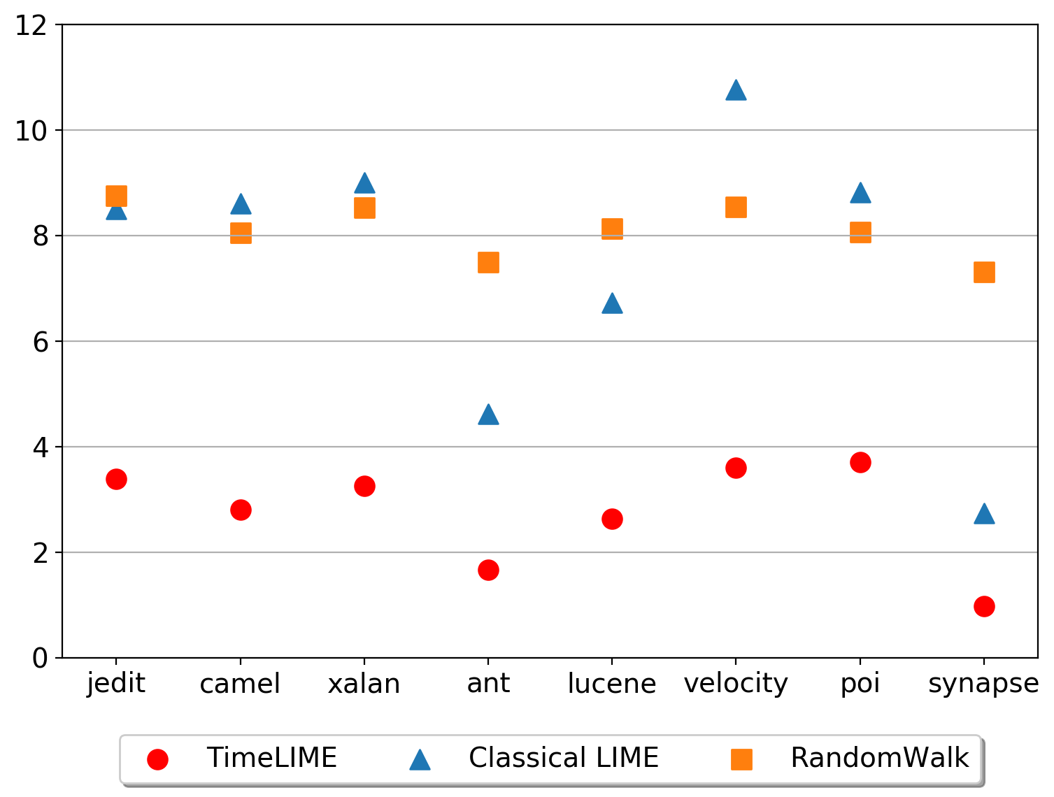
Figure 3. RQ1 results: Mean size of plans across all instances in release $z$. Y-axis= number of features changed by recommended plans. Smaller y-values indicate smaller plans

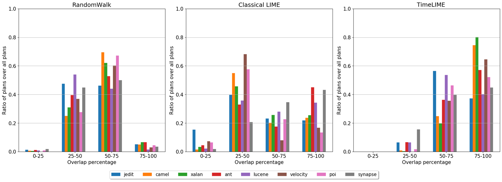
Figure 4. RQ2 results: Distribution of overlap scores of the RandomWalk planner, classical LIME planner, and TimePlanner respectively. Within each of these three plots, results that fall to the right-hand-side are better since they better correspond to actual developer actions. Note that, by this measure, TimeLIME better reflects actual developer changes. In this figure, the x-axis is the overlap scores computed by Eq. 3 and discretized into quantiles. This figure is summarized in Figure 5.

5. Results

RQ1: Are all explanations precedented?

Before doing anything else, we need to assess if there are any differences between the explanations generated by TimeLIME and those of classic LIME. This is important to check since if both algorithms are producing the same recommendations, then there is little point to this paper.

Figure 3 reports the mean size of plans across all instances in release $z$. In terms of the size of the proposed changes, TimeLIME generates much smaller recommendation plans compared to the classical LIME and random planner. Note that since TimeLIME in the experiment restricts recommendations to the top 5 features with highest Hedge’s $g$ scores, the size of an TimeLIME plan will never be more than 5. However, as shown in the figure, the average size of TimeLIME plans is always smaller than 5. This implies that the original explanation sets, returned by the classical LIME, do contain unprecedented explanations which then get rejected by the TimePlanner. Hence we say that

Note that we view this result as a potential flaw in classic-LIME since, as shown below, better explanations arise from using just the precedented attributes.

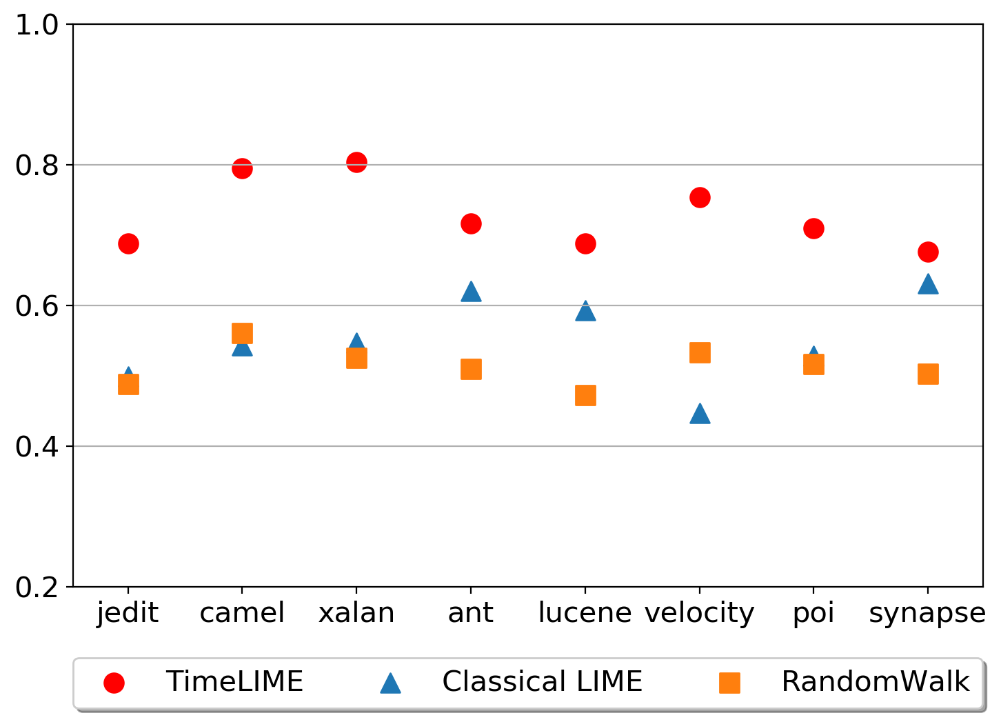
Figure 5. More RQ2 results: The mean overlap scores of all recommendation plans made by 3 planners seen in Figure 4.

RQ2: Do developers prefer precedented explanations?

An explanation/recommendation can be proven useful if there is evidence indicating developers could actually apply those kinds of changes. Figure 4 comments on how often developers are willing to perform the plans suggested by different planners. This figure was generated using the $K$-test procedure described above. The x-axis of that figure shows the $J_{y,z}$ overlap measure from Eq. 3 in §3. The y-axis of that figure shows the portion of plans falling into each overlap score quantile among all plans generated by planners.

In that visual representation, the planners whose actions most correspond to known developer actions have higher values on the right-hand-side of each plot. Such values illustrate examples where changes proposed by the planner most correspond to changes made by the developers. In general, we observe the tendency that the TimePlanner generates plans that are much more favored by developers than the plans from the other 2 planners.

To facilitate the comparison over the planners, Figure 5 lists three sets of average overlap scores for Random, classical LIME, and Refined-LIME:

• The classical LIME recommendations do not correspond well with known developer actions (since the expected overlap score within a project is around 0.5, sometimes even lower).

• The plans provided by the classical LIME have no significant difference ($p<.05$) from RandomWalk.

• Of the 3 planners studied here, TimeLIME’s plans most reflect the actions of developers.

Hence we say:

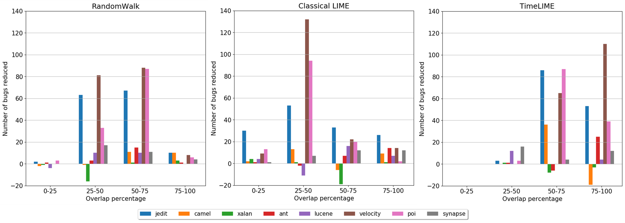
Figure 6. RQ3 results: Total number of bugs reduced by the RandomWalk planner, classical LIME planner, and the TimePlanner respectively. Within each of these three plots, results that fall to the right-hand-side are better since they they most correspond to most defect improvement in the subsequent release. By this measure, TimeLIME is the best since its plans are associated with most defect reduction. In this chart, a positive number implies a reduction of bugs in the validation dataset. A negative number means an increase in the total number of bugs. The sum of 4 bars should be the same within each project despite different planners since the same validation datasets are used. This chart is summarised in Figure 7.

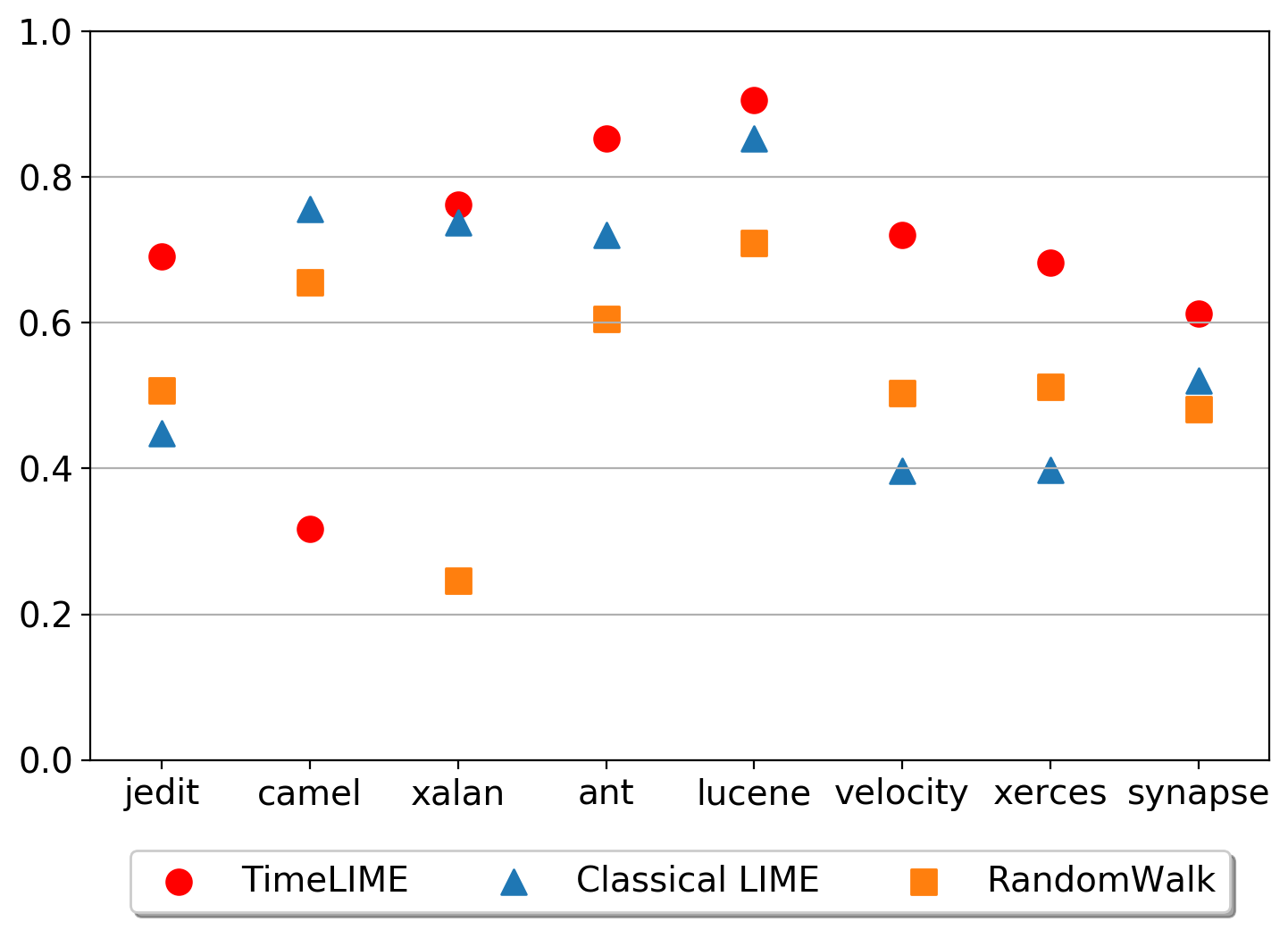
Figure 7. RQ3 results: Summary of Figure 6. The expected values of weighted scores $S_{scaled}$ of 3 planners in each projects as computed by Eq. 5.

RQ3: Are precedented explanations better at defect reduction?

As discussed earlier, better explanations in SE are believed to be explanations that are (a) easier to apply while (b) maintaining the effectiveness in reducing bugs.

The first criterion has already been met. As seen there, the recommendations made by TimeLIME are much smaller, hence easier to apply, than the other methods studied here. Also, as seen above, the recommendations from Refined-LIME correspond to the known actions of developers.

To measure the second criterion, we chose to use a weighted sum function to compute the net gain of each planner. The weighted sum function in Eq. (4) weights the NDPV by the overlap score of the plan.

In the experiment, each plan $p_{i}$ from the all $N$ plans returns an overlap score $s_{i}$ and a NDPV number $n_{i}$ (positive number indicates bugs reduced, negative number indicates bugs added). Then we weight the NDPV $n_{i}$ by the planner by $s_{i}$ to compute the aggregate score $S$.

(4) $$S=\sum{s_{i}*n_{i}}$$

Note that the larger the overlap the greater the change in the number of defects introduced. Equivalently, a very high overlap score of a plan that ends up with new bugs added in the next release implies strong unreliability of this plan. As a result, the planner should receive more scores deducted by this plan.

Additionally, given that the total number of bugs varies from each project as shown in Figure 6, a project with more bugs reduced in the validation dataset will expect the planner to score more than the planner whose validation dataset has fewer bugs reduced so that their performance can be considered proportionally similar. For example, project A has $NDPV=100$ in release $y$ and another project B has $NDPV=10$ in its next release y. If one would like to see similar performance of a planner on these 2 projects, the weighted score in project A $S_{A}$ is expected to be 10 times higher than $S_{B}$ since there are potentially more bugs that can be reduced by a planner in project $A$ than in project $B$ and it won’t make any sense if a planner gains the same score in both projects. From this perspective, we scale the final score $S$ in Eq. 4 by the sum of NDPV within the project to get the scaled score $S_{scaled}$.

(5) $$S_{scaled}=\frac{\sum_{i}^{N}{s_{i}*n_{i}}}{\sum_{i}^{N}{n_{i}}}$$

The visualized result in Figure 7 shows that the TimePlanner obtains highest average $S_{scaled}$ scores in most of the projects (7 out of 8).

As to the one case that failed (CAMEL), we have investigated various reasons why that might be so. Looking at the distributions of its features, we cannot see anything that distinguishes CAMEL from the other projects. The most promising possibility is that the staffing profile of CAMEL changed dramatically during the releases studied here, which means that numerous extra bugs arrived due to the inexperience of the new staff.

Whatever the reason for the CAMEL result, the overall result is very clear:

6. Threats to validity

Due to the complexity of the experiment designed in this case study, there are many factors that can threaten the validity of these results.

6.1. Learner bias

This paper selects RFC as the black-box classifier because prior research has shown that RFC is ranked as one of the top models among all 32 classifiers used in defect prediction. However, the preeminent predictive power of RFC does not ensure that explanations derived from it are preeminent recommendations as well. Other methods from the top rank may be more suitable in the problem of explanation generation while we haven’t explored more.

6.2. Instrument bias

Explainable AI is experiencing its resurgence and various approaches are proposed to generate explanations. Although LIME is one of the widely cited and well-known tools, it is possible other tools are more suitable in solving SE problems, which can make solutions from LIME sub-optimal. Hence, to verify if adding in SE knowledge can always improve AI tools, we need to make a comprehensive exploration that includes more explanation generation methods.

6.3. Evaluation bias

Experimentation in this paper uses performance measures as defined above. Other similarity score functions are also widely used in research. A comprehensive analysis using these measures can be further performed using our replication package. Additionally, other measures can easily be added to extend this replication package.

6.4. Sampling bias

This paper uses historical data analysis to restrain recommendation generation in which 3 releases are collected per project. However, we still prefer to collect more releases of the project and augment the historical data analysis. Recent research in defect prediction has revealed that among several past releases of the project, there exists one bellwether release that is the most suitable training dataset(Krishna and Menzies, 2018). Therefore, we have reasons to believe in a similar conjecture that there exists such bellwether release that is most helpful in fitting the learner and explainer.

7. Future work

For future work, we need to take action to retire the above threats to validity.

7.1. More Learners

More black-box learners should be used in the experiment to construct a more comprehensive comparison. Although the limited sample amount of defect prediction datasets has ruled out many deep learning models such as Neural Network due to the overhead, there are still many other models, including but not limited to Random Subspace Sampling and Sequential Minimal Optimization, applicable for this experiment.

7.2. More Explainers

As described above, LIME is a representative member in the family of local surrogate interpretation models. Other local explanation generation methods that apply tree-structure extraction or association rule mining or so on should also be introduced in the discussion.

7.3. More Data

We would like to collect not only more SE projects of defection prediction data but also more releases of a single project. This can facilitate the further exploration on the accountability of our historical data analysis.

8. Conclusion

When dealing with temporal data (e.g., successive software releases), it is useful to restrict any conclusions to actions that have appeared in the historical record of that project. This paper has compared planners built upon the classical LIME explanations that do/do not respect temporal precedence. We find that plans that respect precedence:

• Are smaller: In terms of the average size of recommended plans. The TimeLIME generally generates smaller plans than the classical LIME and RandomWalk in every project. Smaller plans are preferred to larger plan since the latter can be faster to apply.

• Are preferred by developers: In terms of the overlap between the proposed plans and the developer actions in the upcoming release, plans proposed by TimeLIME better match what developers actually do.

• Are better: In terms of the scaled weighted scores $S_{scaled}$ that indicate the overall net gain received per project. TimeLIME gets the highest score among 3 planner in 7 out of 8 projects (while the classical LIME wins in only 1 project).

In conclusion, we assert two things. Firstly, the above results clearly show that precedented explanations lead to better explanations (and better plans based on those explanations).

Secondly, and more generally, our community should be more careful about using off-the-shelf AI tools without first adapting them using SE knowledge. We think it is rash and ill-advised just to throw standard AI tools at SE problems. Those AI methods can be greatly enhanced via SE knowledge. As shown here, adding that knowledge is not a complex thing to do. Further, once that knowledge is applied, this can result in dramatically better systems.

References

- (1)
- AAAI (1990) AAAI. 1990. AAAI 1990 Spring Symposium Series Reports. AI Magazine 11, 3 (Sep. 1990), 27. https://doi.org/10.1609/aimag.v11i3.848
- Agrawal et al. (2018) A. Agrawal, W. Fu, and T. Menzies. 2018. What is wrong with topic modeling? And how to fix it using search-based software engineering. IST (2018).
- Agrawal and Menzies (2018a) A. Agrawal and T. Menzies. 2018a. Is better data better than better data miners?: on the benefits of tuning smote for defect prediction. In IST. ACM.
- Agrawal and Menzies (2018b) Amritanshu Agrawal and Tim Menzies. 2018b. Is “Better Data” Better than “Better Data Miners”? On the Benefits of Tuning SMOTE for Defect Prediction. In Proceedings of the 40th International Conference on Software Engineering (Gothenburg, Sweden) (ICSE ’18). Association for Computing Machinery, New York, NY, USA, 1050–1061. https://doi.org/10.1145/3180155.3180197
- Arcuri and Briand (2011) A. Arcuri and L. Briand. 2011. A practical guide for using statistical tests to assess randomized algorithms in software engineering. In ICSE. IEEE.
- Bird et al. (2009) C. Bird, N. Nagappan, H. Gall, B. Murphy, and P. Devanbu. 2009. Putting It All Together: Using Socio-technical Networks to Predict Failures. In ISSRE.
- Briand et al. (1993) Lionel C Briand, VR Brasili, and Christopher J Hetmanski. 1993. Developing interpretable models with optimized set reduction for identifying high-risk software components. IEEE Transactions on Software Engineering 19, 11 (1993), 1028–1044.
- Chawla et al. (2002) Nitesh V Chawla, Kevin W Bowyer, Lawrence O Hall, and W Philip Kegelmeyer. 2002. SMOTE: synthetic minority over-sampling technique. Journal of artificial intelligence research 16 (2002), 321–357.
- Chen et al. (2018) Di Chen, Wei Fu, Rahul Krishna, and Tim Menzies. 2018. Applications of Psychological Science for Actionable Analytics. Foundations of Software Engineering (2018).
- Clancey (1994) William J. Clancey. 1994. Notes on “Epistemology of a Rule-Based Expert System”. MIT Press, Cambridge, MA, USA, 197–204.
- Couto et al. (2014) Cesar Couto, Pedro Pires, Marco Tulio Valente, Roberto S Bigonha, and Nicolas Anquetil. 2014. Predicting software defects with causality tests. Journal of Systems and Software 93 (2014), 24–41.
- Fu et al. (2016) W. Fu, T. Menzies, and X. Shen. 2016. Tuning for software analytics: Is it really necessary? IST (2016).
- Ghotra et al. ([n.d.]) B. Ghotra, S. McIntosh, and A. E. Hassan. [n.d.]. Revisiting the Impact of Classification Techniques on the Performance of Defect Prediction Models. In 2015 37th ICSE.
- Ghotra et al. (2015) Baljinder Ghotra, Shane McIntosh, and Ahmed E Hassan. 2015. Revisiting the impact of classification techniques on the performance of defect prediction models. In Proceedings of the 37th International Conference on Software Engineering-Volume 1. IEEE Press, 789–800.
- Hihn and Menzies (2015) Jaitus Hihn and Tim Menzies. 2015. Data mining methods and cost estimation models: Why is it so hard to infuse new ideas?. In Automated Software Engineering Workshop (ASEW), 2015 30th IEEE/ACM International Conference on. IEEE, 5–9.
- Ho (1995) Tin Kam Ho. 1995. Random decision forests. In Proceedings of 3rd international conference on document analysis and recognition, Vol. 1. IEEE, 278–282.
- Jureczko (2011) Marian Jureczko. 2011. Significance of different software metrics in defect prediction. Software Engineering: An International Journal 1, 1 (2011), 86–95.
- Jureczko and Madeyski (2010) Marian Jureczko and Lech Madeyski. 2010. Towards identifying software project clusters with regard to defect prediction. In Proceedings of the 6th International Conference on Predictive Models in Software Engineering. 1–10.
- Jureczko and Spinellis (2010) Marian Jureczko and Diomidis Spinellis. 2010. Using object-oriented design metrics to predict software defects. Models and Methods of System Dependability. Oficyna Wydawnicza Politechniki Wrocławskiej (2010), 69–81.
- Kampenes et al. (2007) Vigdis By Kampenes, T. Dybå, J. Erskine Hannay, and D. I. K. Sjøberg. 2007. A Systematic Review of Effect Size in Software Engineering Experiments. IST (2007).
- Khoshgoftaar et al. (1998) Taghi M Khoshgoftaar, Edward B Allen, Robert Halstead, Gary P Trio, and Ronald M Flass. 1998. Using process history to predict software quality. Computer 31, 4 (1998), 66–72.
- Krishna and Menzies (2017) Rahul Krishna and Tim Menzies. 2017. Learning Actionable Analytics from Multiple Software Projects. arXiv preprint arXiv:1708.05442 (2017).
- Krishna and Menzies (2018) Rahul Krishna and Tim Menzies. 2018. Bellwethers: A baseline method for transfer learning. IEEE Transactions on Software Engineering 45, 11 (2018), 1081–1105.
- Leake (1991) David B. Leake. 1991. Goal-Based Explanation Evaluation. Cognitive Science 15, 4 (1991), 509–545. https://doi.org/10.1207/s15516709cog1504_2
- Madeyski and Jureczko (2015) Lech Madeyski and Marian Jureczko. 2015. Which process metrics can significantly improve defect prediction models? An empirical study. Software Quality Journal 23, 3 (2015), 393–422.
- Menzies et al. (2002) Tim Menzies, Robert F. Cohen, Sam Waugh, and Simon Goss. 2002. Applications of Abduction: Testing Very Long Qualitative Simulations. IEEE Trans. on Knowl. and Data Eng. 14, 6 (Nov. 2002), 1362–1375. https://doi.org/10.1109/TKDE.2002.1047773
- Menzies et al. (2007) T. Menzies, J. Greenwald, and A. Frank. 2007. Data Mining Static Code Attributes to Learn Defect Predictors. TSE (2007).
- Menzies et al. (2010) T. Menzies, Z. Milton, B. Turhan, B. Cukic, Y. Jiang, and A. Bener. 2010. Defect Prediction from Static Code Features: Current Results, Limitations, New Approaches. ASE (2010).
- Mueller et al. (2019) Shane T. Mueller, Robert R. Hoffman, William Clancey, Abigail Emrey, and Gary Klein. 2019. Explanation in Human-AI Systems: A Literature Meta-Review, Synopsis of Key Ideas and Publications, and Bibliography for Explainable AI. arXiv:cs.AI/1902.01876
- Nagappan and Ball (2005) Nachiappan Nagappan and Thomas Ball. 2005. Static analysis tools as early indicators of pre-release defect density. In Proceedings. 27th International Conference on Software Engineering, 2005. ICSE 2005. IEEE, 580–586.
- Nam et al. (2018) J. Nam, W. Fu, S. Kim, T. Menzies, and L. Tan. 2018. Heterogeneous Defect Prediction. IEEE TSE (2018).
- Rahman et al. (2014) F. Rahman, S. Khatri, E. T Barr, and P. Devanbu. 2014. Comparing static bug finders and statistical prediction. In ICSE. ACM.
- Ribeiro et al. (2016) Marco Tulio Ribeiro, Sameer Singh, and Carlos Guestrin. 2016. ” Why should i trust you?” Explaining the predictions of any classifier. In Proceedings of the 22nd ACM SIGKDD international conference on knowledge discovery and data mining. 1135–1144.
- Ribeiro et al. (2018) Marco Tulio Ribeiro, Sameer Singh, and Carlos Guestrin. 2018. Anchors: High-precision model-agnostic explanations. In Thirty-Second AAAI Conference on Artificial Intelligence.
- Rosen et al. (2015) C. Rosen, B. Grawi, and E. Shihab. 2015. Commit Guru: Analytics and Risk Prediction of Software Commits (ESEC/FSE 2015).
- Rosenthal et al. (1994) Robert Rosenthal, Harris Cooper, and L Hedges. 1994. Parametric measures of effect size. The handbook of research synthesis 621, 2 (1994), 231–244.
- Shihab et al. (2010) Emad Shihab, Zhen Ming Jiang, Walid M Ibrahim, Bram Adams, and Ahmed E Hassan. 2010. Understanding the impact of code and process metrics on post-release defects: a case study on the eclipse project. In Proceedings of the 2010 ACM-IEEE International Symposium on Empirical Software Engineering and Measurement. 1–10.
- Shin and Williams (2013) Y. Shin and L. Williams. 2013. Can traditional fault prediction models be used for vulnerability prediction? EMSE (2013). https://doi.org/10.1007/s10664-011-9190-8
- Witten et al. (2011) I. H. Witten, E. Frank, and M. A. Hall. 2011. Data Mining: Practical Machine Learning Tools and Techniques (3rd ed.). Morgan Kaufmann Publishers Inc., San Francisco, CA, USA.