On the last zero process with applications in corporate bankruptcy

Abstract

For a spectrally negative Lévy process $X$, consider $g_{t}$, the last time $X$ is below the level zero before time $t\geq 0$. We use a perturbation method for Lévy processes to derive an Itô formula for the three-dimensional process $\{(g_{t},t,X_{t}),t\geq 0\}$ and its infinitesimal generator. Moreover, with $U_{t}:=t-g_{t}$, the length of a current positive excursion, we derive a general formula that allows us to calculate a functional of the whole path of $(U,X)=\{(U_{t},X_{t}),t\geq 0\}$ in terms of the positive and negative excursions of the process $X$. As a corollary, we find the joint Laplace transform of $(U_{\textbf{e}_{q}},X_{\textbf{e}_{q}})$, where $\textbf{e}_{q}$ is an independent exponential time, and the q-potential measure of the process $(U,X)$. Furthermore, using the results mentioned above, we find a solution to a general optimal stopping problem depending on $(U,X)$ with some applications for corporate bankruptcy. Lastly, we establish a link between the optimal prediction of $g_{\infty}$ and optimal stopping problems in terms of $(U,X)$ as per Baurdoux and Pedraza, 2020a .

Keywords: Lévy processes, last zero, positive excursions, Itô formula, optimal stopping.

Mathematics Subject Classification (2020): 60G40, 60G51, 60J35

1 Introduction

Last passage times have received considerable attention in the recent literature. For instance, in the classic ruin theory (which describes the capital of an insurance company), the moment of ruin is considered as the first time the process is below level zero. However, in more recent literature, the last passage time below zero is treated as the moment of ruin and the Cramér–Lundberg has been generalised to spectrally negative Lévy processes (see e.g. Chiu and Yin, (2005)). Moreover, in Paroissin and Rabehasaina, (2013), spectrally positive Lévy processes are used for degradation models, and the last passage time above a fixed boundary is considered the failure time.

Let $X=\{X_{t},t\geq 0\}$ be a spectrally negative Lévy process. For any $t\geq 0$ and $x\in\mathbb{R}$, we define $g_{t}^{(x)}$ as the last time that the process is below $x$ before time $t$, i.e.,

$$g_{t}^{(x)}=\sup\{0\leq s\leq t:X_{s}\leq x\},$$

with the convention $\sup\emptyset=0$. We simply denote $g_{t}:=g_{t}^{(0)}$ for all $t\geq 0$.

A similar version of this random time is studied in Revuz and Yor, (1999) (see Chapter XII.3), namely the last hitting time at zero, before any time $t\geq 0$, to describe excursions straddling a given time. It is also shown that this random time at time $t=1$ follows the arcsine distribution. The last-hitting time of zero has some play an essential role in the study of Azéma’s martingale (see Azéma and Yor, (1989)). In Salminen, (1988), the distribution of the last hitting time of a moving boundary is found.

It is well know that spectrally negative Lévy processes are often used to model the surplus of an insurance company (see e.g. Huzak et al., 2004a , Huzak et al., 2004b , Chan, (2004), Klüppelberg et al., (2004), among many others). The random variable $g_{t}$ provides essential information regarding the insurance company’s solvency. For instance, a large value of $U_{t}:=t-g_{t}$ (the time of the current positive excursion away from zero) indicates that the insurance company’s capital has not fallen below zero for a considerable amount of time, suggesting that the company is currently able to meet debts and financial obligations.

Lévy processes are also widely used in financial modelling. For instance, there is considerable work in the literature that adopts markets driven by Lévy processes (see e.g. Schoutens, (2003), Cont and Tankov, (2003), Kyprianou et al., (2006), among many others). Assume that a stock price is given by $Y_{t}=\exp(X_{t})$, then it is of interest for an investor to know when is the last time, before the time $t\geq 0$, that the stock price is below a certain level $y^{*}>0$. That is, the investor is interested in knowing the value of $g_{t}^{(\log(y^{*}))}$.

In Leland, (1994) and Manso et al., (2010), it is assumed that equity holders endogenously choose the time of the bankruptcy of a firm. They suppose that the performance measure of the firm can be modelled by a time-homogeneous diffusion $Y=\{Y_{t},t\geq 0\}$. Then, the time of the bankruptcy is determined by the optimal stopping problem

$$\sup_{\tau\in\mathcal{T}}\mathbb{E}\left(\int_{0}^{\tau}e^{-rt}[\delta(Y_{t})-c(Y_{t})]\textup{d}t\bigg{|}Y_{t}=y\right),$$

where $c(y)$ is the coupon rate that the firm must pay to the debt holders and $\delta(y)$ is the payout rate received by the firm. The performance $Y$ measures the ability of the firm to serve its future debt obligations and can be taken to be financial ratios, stock prices or credit ratings. Note that given a certain level $k\geq 0$, the current positive excursion above the level $k$, given by $V_{t}^{(k)}=t-\sup\{0\leq s\leq t:Y_{s}\geq k\}$, also provides information about the performance of the firm. Indeed, large values of $V_{t}^{(k)}$ suggest that the firm has been able to meet its obligations for a long time without a negative dividend rate. Hence, the default time of the firm can be generalised to consider the process $(V,Y)=\{(V_{t},Y_{t}),t\geq 0\}$ as its performance measure, where $Y$ can be taken to be an exponential Lévy process.

On the other hand, when pricing of American-type options is necessary to solve optimal stopping problems (see e.g. Jacka, (1991), Mordecki, (1999), Mordecki, (2002) and Kyprianou et al., (2006)), and it is known that they are intimately related to free-boundary problems (see e.g. Chapter III in Peskir and Shiryaev, (2006)). Then, their solution often requires techniques that involve a Markovian approach and applications of Itô formula. Hence, an explicit expression of the infinitesimal generator of the process is needed. Moreover, in more recent literature, the development of fluctuations identities allowed the use of the “guess and verify” approach to solving optimal stopping problems driven by Lévy processes (see, for example, Avram et al., (2004), Alili and Kyprianou, (2005) and Kyprianou and Surya, (2005)). Hence, given the importance of the random time $g_{t}$, it is relevant to be able to solve optimal stopping problems of the form,

$$\sup_{\tau\in\mathcal{T}}\mathbb{E}\left(e^{-r\tau}f(g_{\tau},\tau,X_{\tau})+\int_{0}^{\tau}e^{-r\tau}G(g_{s},s,X_{s})\textup{d}s\right).$$

Indeed, in Baurdoux and Pedraza, 2020a , an optimal stopping of the form above arises when predicting $g_{\infty}$ with stopping times in an $L_{p}$ sense. In Section 4.1, we also propose an optimal stopping problem that generalises the work of Leland, (1994) and Manso et al., (2010) on corporate bankruptcy. Hence, it is relevant to derive path properties of the process $\{(g_{t},t,X_{t}),t\geq 0\}$.

The process $\{g_{t},t\geq 0\}$ is non-decreasing and hence is a process of finite variation, implying that it belongs to the class of semi-martingales. Then Itô formula for the process $\{(g_{t},t,X_{t}),t\geq 0\}$ is well known (see e.g. Protter, (2005), Theorem 33) and is given for any function $F:\mathbb{R}^{3}\mapsto\mathbb{R}$ in $C^{1,1,i}$, where $i=2$ if $X$ is of infinite variation, and $i=1$ otherwise, by

$$F(g_{t},t,X_{t})$$

$$=F(g_{0},0,X_{0})+\int_{0}^{t}\frac{\partial}{\partial\gamma}F(g_{s-},s,X_{s-})\textup{d}g_{s}+\int_{0}^{t}\frac{\partial}{\partial t}F(g_{s},s,X_{s})\textup{d}s$$

$$\qquad+\int_{0}^{t}\frac{\partial}{\partial x}F(g_{s-},s,X_{s-})\textup{d}X_{s}+\frac{1}{2}\sigma^{2}\int_{0}^{t}\frac{\partial^{2}}{\partial x^{2}}F(g_{s},s,X_{s})\textup{d}s$$

$$\qquad+\sum_{0<s\leq t}\left(F(g_{s},s,X_{s})-F(g_{s-},s,X_{s-})-\frac{\partial}{\partial\gamma}F(g_{s-},s,X_{s-})\Delta g_{s}-\frac{\partial}{\partial x}F(g_{s-},s,X_{s-})\Delta X_{s}\right).$$

Note that the formula above is given in terms of the jumps of the processes $\{g_{t},t\geq 0\}$ and $X$, and it does not reflect the dependence between $g_{t}$ and $X_{t}$. Indeed, some of the jumps of $\{g_{t},t\geq 0\}$ occur when $X$ jumps to $(-\infty,0)$ from the positive half line. Moreover, when a Brownian motion component is included in the dynamics of $X$, the stochastic process $\{g_{t},t\geq 0\}$ has infinitely many (small) jumps due to creeping. These facts imply that, to obtain a more explicit version of Itô formula, a careful study of the trajectory of $t\mapsto g_{t}$ is required in terms of the excursions of $X$ away from zero.

On the other hand, it turns out that $\{(g_{t},t,X_{t}),t\geq 0\}$ belongs to the family of strong Markov processes (see Proposition 3.1). Hence, a general form of its infinitesimal generator is known. For instance, from the general theory of Markov processes (see Dynkin, (1965)), we know that if $Z$ is a strong Markov process in $\mathbb{R}^{d}$, with $d$ a positive integer, and if $B\subset\mathbb{R}^{d}$ is any relative compact set, there exist functions $\sigma_{ij}$, $b_{i}$ and $c$ on $B$ and a kernel $\nu$ such that for any function $F\in C^{2}$ with compact support and $z\in B$,

$$\mathcal{A}_{Z}F(z) =c(z)F(z)+\sum_{i=1}^{d}b_{i}(z)\frac{\partial}{\partial z_{i}}F(z)+\sum_{i,j=1}^{d}\sigma_{ij}(z)\frac{\partial^{2}}{\partial z_{i}\partial z_{j}}F(z)$$

$$\qquad+\int_{\mathbb{R}^{d}\setminus\{0\}}\left(F(y)-F(z)-\sum_{i=1}^{d}(y_{i}-z_{i})\frac{\partial}{\partial z_{i}}F(z)\right)\nu(z,\textup{d}y).$$

However, more explicit expressions for Itô formula and the infinitesimal generator are required in applications (for example, in optimal stopping and free boundary problems). In this work (see Theorem 3.3 and Corollary 3.5), we give an expression for Itô formula and the infinitesimal generator of the process $\{(t,g_{t},X_{t}),t\geq 0\}$ in terms of the dynamics of $X$ only.

We also consider, for any $t\geq 0$, the random variable $U_{t}=t-g_{t}$, the time of the current positive excursion away from zero. Then, having in mind the derivation of expressions for the potential measure of $(U,X)=\{(U_{t},X_{t}),t\geq 0\}$ and its joint Laplace transform at an exponential time, we also derive an explicit formula, in terms of the positive and negative excursions of $X$, for functionals of the process $(U,X)$ of the form

$$\mathbb{E}_{u,x}\left(\int_{0}^{\infty}e^{-qr}K(U_{r},X_{r})\textup{d}r\right),$$

for some function $K$ satisfying some conditions (see Theorem 3.6), where $q\geq 0$ and $\mathbb{P}_{u,x}$ is the measure for which $(U_{0},X_{0})=(u,x)$ in view of the Markov property of $(U,X)$. The reader can find applications of these results in Baurdoux and Pedraza, 2020a , which concerns the optimal prediction of the last zero of a spectrally negative Lévy process and where the solution is given in terms of the process $(U,X)$. We also apply these results in Section 4 to solve a general optimal stopping problem.

This paper is organised as follows. In Section 2, we collect some fluctuation identities of spectrally negative Lévy processes. Section 3 is dedicated to defining the last zero process, for which its basic properties are shown. Moreover, a derivation of Itô formula, infinitesimal generator and formula for the expectation of a functional of $(U,X)$ are the main results of this section (see Theorems 3.3 and 3.6 and Corollary 3.5). Then, the results mentioned above are applied to find formulas for the joint Laplace transform of $(U,X)$ at an exponential time, and a density of its $q$-potential measure is found. In Section 4, we solve an optimal stopping theorem (see Theorem 4.1) driven by $(U,X)$. In particular, in Example 4.2, we propose an optimal stopping problem applied to corporate bankruptcy that depends on the trajectory of $(U,X)$. We also describe some optimal prediction problems of the last zero of the process. In this section, we emphasise the importance of the results developed in Section 3. Lastly, in Section 5, we include the main proofs of the paper.

2 Preliminaries

Let $(\Omega,\mathcal{F},\mathbb{F},\mathbb{P})$ be a filtered probability space, where $\mathbb{F}=\{\mathcal{F}_{t},t\geq 0\}$ is a filtration which is naturally enlarged (see Definition 1.3.38 of Bichteler, (2002)). A Lévy process $X=\{X_{t},t\geq 0\}$ is an almost surely càdlàg process that has independent and stationary increments such that $\mathbb{P}(X_{0}=0)=1$. From the stationary and independent increments property, the law of $X$ is characterised by the distribution of $X_{1}$. We hence define the characteristic exponent of $X$, $\Psi(\theta):=-\log(\mathbb{E}(e^{i\theta X_{1}}))$. The Lévy–Khintchine formula guarantees the existence of constants, $\mu\in\mathbb{R}$, $\sigma\geq 0$ and a measure $\Pi$ concentrated on $\mathbb{R}\setminus\{0\}$ with the property that $\int_{\mathbb{R}}(1\wedge x^{2})\Pi(\textup{d}x)<\infty$ (called the Lévy measure) such that

$$\Psi(\theta)=i\mu\theta+\frac{1}{2}\sigma^{2}\theta^{2}-\int_{\mathbb{R}}(e^{i\theta y}-1-i\theta y\mathbb{I}_{\{|y|<1\}})\Pi(\textup{d}y).$$

Moreover, from the Lévy–Itô decomposition we can write

$$X_{t}=\sigma B_{t}-\mu t+\int_{[0,t]}\int_{(-\infty,-1)\cup(1,\infty)}xN(\textup{d}s\times\textup{d}x)+\int_{[0,t]}\int_{(-1,1)}x(N(\textup{d}s\times\textup{d}x)-\textup{d}s\Pi(\textup{d}x)),$$

where $N$ is a Poisson random measure on $\mathbb{R}^{+}\times\mathbb{R}$ with intensity $\textup{d}t\times\Pi(\textup{d}x)$ and $B=\{B_{t},t\geq 0\}$ is an independent standard Brownian motion. We state now some properties and facts about Lévy processes. The reader can refer, for example, to Bertoin, (1998), Sato, (1999) and Kyprianou, (2014) for more details. Every Lévy process $X$ is also a strong Markov $\mathbb{F}$-adapted process. For all $x\in\mathbb{R}$, denote $\mathbb{P}_{x}$ as the law of $X$ when started at the point $x\in\mathbb{R}$, that is, $\mathbb{E}_{x}(\cdot)=\mathbb{E}(\cdot|X_{0}=x)$. Due to the spatial homogeneity of Lévy processes, the law of $X$ under $\mathbb{P}_{x}$ is the same as that of $X+x$ under $\mathbb{P}$.

The process $X$ is a spectrally negative Lévy process if it has no positive jumps ($\Pi(0,\infty)=0$) with no monotone paths. We state now some important properties and fluctuation identities of spectrally negative Lévy processes, which will be useful in later sections, see Bertoin, (1998), Chapter VII or Chapter 8 in Kyprianou, (2014) for details.

Due to the absence of positive jumps, we can define the Laplace transform of $X_{1}$. We denote $\psi(\beta)$ as the Laplace exponent of the process, that is, $\psi(\beta)=\log(\mathbb{E}(e^{\beta X_{1}}))$. Then for all $\beta\geq 0$,

$$\psi(\beta)=-\mu\beta+\frac{1}{2}\sigma^{2}\beta^{2}+\int_{(-\infty,0)}(e^{\beta y}-1-\beta y\mathbb{I}_{\{y>-1\}})\Pi(\textup{d}y).$$

It can be shown that $\psi$ is an infinitely differentiable and strictly convex function on $(0,\infty)$ that tends to infinity at infinity. In particular, $\psi^{\prime}(0+)=\mathbb{E}(X_{1})\in[-\infty,\infty)$ and determines the value of $X$ at infinity. When $\psi^{\prime}(0+)>0$ the process $X$ drifts to infinity, i.e., $\lim_{t\rightarrow\infty}X_{t}=\infty$, when $\psi^{\prime}(0+)<0$, $X$ drifts to minus infinity and the condition $\psi^{\prime}(0+)=0$ implies that $X$ oscillates, that is, $\limsup_{t\rightarrow\infty}X_{t}=-\liminf_{t\rightarrow\infty}X_{t}=\infty$. We also define the right-inverse of $\psi$,

$$\Phi(q)=\sup\{\beta\geq 0:\psi(\beta)=q\},\qquad q\geq 0.$$

The process $X$ has paths of finite variation if and only if $\sigma=0$ and $\int_{(-1,1)}|x|\Pi(\textup{d}x)<\infty$, otherwise $X$ has paths of infinite variation. In the latter case, we have that $X$ can be just simply written as a drift process minus a subordinator,

$$X_{t}=dt+\int_{[0,t]}\int_{(-\infty,0)}xN(\textup{d}s\times\textup{d}x),$$

where

$$d=-\mu-\int_{(-1,0)}x\Pi(\textup{d}x).$$

Note that, since $X$ cannot have monotone paths, we necessarily have that $d>0$. Define $\tau_{a}^{+}$ as the first passage time above the level $a>0$,

$$\tau_{a}^{+}=\inf\{t>0:X_{t}>a\}.$$

Then, for any $a>0$ and $q\geq 0$, the Laplace transform of $\tau_{a}^{+}$ is given by

$$\mathbb{E}(e^{-q\tau_{a}^{+}}\mathbb{I}_{\{\tau_{a}^{+}<\infty\}})=e^{-\Phi(q)a}.$$ (1)

An essential family of functions for spectrally negative Lévy processes are the scale functions, $W^{(q)}$. For all $q\geq 0$, the scale function $W^{(q)}:\mathbb{R}\mapsto\mathbb{R}_{+}$ is such that $W^{(q)}(x)=0$ for all $x<0$ and it is characterised on the interval $[0,\infty)$ as a strictly increasing and continuous function with Laplace transform given by

$$\int_{0}^{\infty}e^{-\beta x}W^{(q)}(x)\textup{d}x=\frac{1}{\psi(\beta)-q},\qquad\text{ for }\beta>\Phi(q).$$ (2)

For the case $q=0$ we simply denote $W=W^{(0)}$. When $X$ has paths of infinite variation, $W^{(q)}$ is continuous on $\mathbb{R}$ and $W^{(q)}(0)=0$ for all $q\geq 0$, otherwise, we have $W^{(q)}(0)=1/d$, where $d>0$. The behaviour of $W^{(q)}$ at infinity is the following. For $q\geq 0$ we have, $\lim_{x\rightarrow\infty}e^{-\Phi(q)x}W^{(q)}(x)=\Phi^{\prime}(q)$.

There are some important fluctuation identities of Lévy processes in terms of the scale functions. In particular, we list some that will be useful in later sections. Denote by $\tau_{x}^{-}$ as the first time $X$ is strictly below the level $x\leq 0$, i.e.,

$$\tau_{x}^{-}=\inf\{t>0:X_{t}<x\}.$$

The Laplace transform of $\tau_{a}^{+}$, on the event of hitting the level $a>0$ before entering the set $(-\infty,0)$, is given by

$$\mathbb{E}_{x}\left(e^{-q\tau_{a}^{+}}\mathbb{I}_{\{\tau_{a}^{+}<\tau_{0}^{-}\}}\right)=\frac{W^{(q)}(x)}{W^{(q)}(a)}$$ (3)

for any $x\leq a$. The joint Laplace transform of $\tau_{0}^{-}$ and $X_{\tau_{0}^{-}}$ is

$$\mathbb{E}_{x}(e^{-q\tau_{0}^{-}+\beta X_{\tau_{0}^{-}}}\mathbb{I}_{\{\tau_{0}^{-}<\infty\}})=e^{\beta x}\mathcal{I}^{(q,\beta)}(x)$$ (4)

for all $x>0$, $q\geq 0$ and $\beta\geq 0$, where the function $\mathcal{I}^{(q,\beta)}$ is given by

$$\mathcal{I}^{(q,\beta)}(x):=1+(q-\psi(\beta))\int_{0}^{x}e^{-\beta y}W^{(q)}(y)\textup{d}y-\frac{q-\psi(\beta)}{\Phi(q)-\beta}e^{-\beta x}W^{(q)}(x),\qquad x\in\mathbb{R}.$$ (5)

When $\beta=\Phi(q)$, for some $q\geq 0$, we understand the equation above in the limiting sense, i.e.,

$$\mathcal{I}^{(q,\Phi(q))}(x)=1-\psi^{\prime}(\Phi(q)+)e^{-\Phi(q)x}W^{(q)}(x),\qquad x\in\mathbb{R}.$$

Since $X$ has only negative jumps, we have that it only creeps upwards, that is,

$$\mathbb{P}(X_{\tau_{x}^{+}}=x,\tau_{x}^{+}<\infty)=1$$ (6)

for any $x>0$. Moreover, $X$ creeps downwards if and only if $\sigma>0$ and we have

$$\mathbb{P}_{x}(X_{\tau_{0}^{-}}=0,\tau_{0}^{-}<\infty)=\frac{\sigma^{2}}{2}\left(W^{\prime}(x)-\Phi(0)W(x)\right)$$ (7)

for any $x>0$. Denote by $\sigma_{x}^{-}$ the first time the process $X$ is below or equal to the level $x$, that is,

$$\sigma_{x}^{-}=\inf\{t>0:X_{t}\leq x\}.$$ (8)

For $t\geq 0$, let $\underline{X}_{t}=\inf_{0\leq s\leq t}X_{s}$ and let $\textbf{e}_{q}$ be an exponential random variable with mean $1/q$, for $q\geq 0$. Since

$$\mathbb{E}(e^{-q\sigma_{x}^{-}}\mathbb{I}_{\{\sigma_{x}^{-}<\infty\}})=\mathbb{P}(\textbf{e}_{q}>\sigma_{x}^{-})=\mathbb{P}(\underline{X}_{\textbf{e}_{q}}\leq-x)$$

for all $x\leq 0$, and the fact that the random variable $\underline{X}_{\textbf{e}_{q}}$ is continuous on $(-\infty,0)$, we have that, for any $x>0$, the stopping times $\sigma_{x}^{-}$ and $\tau_{x}^{-}$ have the same distribution. When $X$ is of infinite variation, $X$ enters instantly to the set $(-\infty,0)$, whilst in the finite variation case, there is a positive time before the process enters it. That implies that in the infinite variation case, $\tau_{0}^{-}=\sigma_{0}^{-}=0$ almost surely. Note that in the finite variation case, since $0$ is irregular for $(-\infty,0]$ (see discussion in Kyprianou, (2014) on p. 157) and due to equation (7), we have that $\sigma_{0}^{-}=\tau_{0}^{-}>0$ a.s.

Let $q>0$ and $a\in\mathbb{R}$. The $q$-potential measure of $X$ killed on exiting $(-\infty,a]$ is absolutely continuous with respect to Lebesgue measure with a density given by

$$e^{-\Phi(q)(a-x)}W^{(q)}(a-y)-W^{(q)}(x-y),\qquad x,y\leq a.$$ (9)

Similarly, the $q$-potential measure of $X$ killed on exiting $[0,\infty)$

$$\int_{0}^{\infty}e^{-qt}\mathbb{P}_{x}(X_{t}\in\textup{d}y,t<\tau_{0}^{-})\textup{d}t$$

is absolutely continuous with respect to Lebesgue measure, and it has a density given by

$$e^{-\Phi(q)y}W^{(q)}(x)-W^{(q)}(x-y)\qquad x,y\geq 0.$$ (10)

Finally, we have that the stochastic process

$$\{e^{-q(t\wedge\tau_{0}^{-}\wedge\tau_{a}^{+})}W^{(q)}(X_{t\wedge\tau_{0}^{-}\wedge\tau_{a}^{+}}),t\geq 0\}$$

is a martingale under $\mathbb{P}_{x}$, for any $a\in(0,\infty]$, $q\geq 0$ and $x\in\mathbb{R}$.

3 The last zero process

Let $X$ be a spectrally negative Lévy process. Recall that $g_{t}^{(x)}$ is the last time that the process is below $x$ before time $t$, i.e.,

$$g_{t}^{(x)}=\sup\{0\leq s\leq t:X_{s}\leq x\},$$

with the convention $\sup\emptyset=0$. We simply denote $g_{t}:=g_{t}^{(0)}$, for all $t\geq 0$. For any stopping time $\tau$, the random variable $g_{\tau}^{(x)}$ is $\mathcal{F}_{\tau}$ measurable. In particular we get that $\{g_{t}^{(x)},t\geq 0\}$ is adapted to the filtration $\{\mathcal{F}_{t},t\geq 0\}$. Moreover, It is easy to show that for a fixed $x\in\mathbb{R}$, the stochastic process $\{g_{t}^{(x)},t\geq 0\}$ is non-decreasing, right-continuous with left limits. Similarly, for a fixed $t\geq 0$, the mapping $x\mapsto g_{t}^{(x)}$ is non-decreasing and almost surely right-continuous with left limits.

It can be easily seen that the process $\{g_{t},t\geq 0\}$ is not a Markov process, particularly not a Lévy process. However, the strong Markov property holds for the three-dimensional process $\{(g_{t},t,X_{t}),t\geq 0\}$.

Proposition 3.1.

The process $\{(g_{t},t,X_{t}),t\geq 0\}$ is a strong Markov process with respect to the filtration $\{\mathcal{F}_{t},t\geq 0\}$ with state space given by $E_{g}=\{(\gamma,t,x):0\leq\gamma<t\text{ and }x>0\}\cup\{(\gamma,t,x):0\leq\gamma=t\text{ and }x\leq 0\}$.

Proof.

From the definition of $g_{t}$, it is easy to note that for all $t\geq 0$, we have $X_{t}\leq 0$ if and only if $g_{t}=t$, from which we obtain that $(g_{t},t,X_{t})$ can take only values in $E_{g}$. Now we proceed to show the strong Markov property holds. Consider a measurable positive function $h:E_{g}\mapsto\mathbb{R}$. Then, we have for any stopping time $\tau$ and $s\geq 0$,

$$\mathbb{E}(h(g_{\tau+s},\tau+s,X_{\tau+s})|\mathcal{F}_{\tau}) =\mathbb{E}(h(g_{\tau}\vee\sup\{r\in[\tau,s+\tau]:X_{r}\leq 0\},\tau+s,X_{\tau+s})|\mathcal{F}_{\tau})$$

$$=\mathbb{E}(h(g_{\tau}\vee\sup\{r\in[\tau,s+\tau]:\widetilde{X}_{r-\tau}+X_{\tau}\leq 0\},\tau+s,\widetilde{X}_{s}+X_{\tau})|\mathcal{F}_{\tau}),$$

where $\widetilde{X}_{r}=X_{r+\tau}-X_{\tau}$ and $a\vee b:=\max\{a,b\}$ for any $a,b\in\mathbb{R}$. Using the strong Markov property of Lévy processes and the fact that $g_{\tau}$ and $X_{\tau}$ are $\mathcal{F}_{\tau}$ measurable we obtain that

$$\mathbb{E}(h(g_{\tau+s},\tau+s,X_{\tau+s})|\mathcal{F}_{\tau})=f_{s}(g_{\tau},\tau,X_{\tau}),$$

where for any $x\in\mathbb{R}$ and $0\leq\gamma\leq t$, the function $f_{s}$ is given by

$$f_{s}(\gamma,t,x) =\mathbb{E}_{x}(h(\gamma\vee\sup\{r\in[t,s+t]:X_{r-t}\leq 0\},t+s,X_{s})).$$

Note that, in the event $\{\sigma_{0}^{-}>s\}$, the set $\{r\in[t,s+t]:X_{r-t}\leq 0\}=\emptyset$. Then, $\gamma\vee\sup\{r\in[t,s+t]:X_{r-t}\leq 0\}=\gamma$, where we used the convention that $\sup\emptyset=0$. Otherwise, in the event $\{\sigma_{0}^{-}\leq s\}$, we have that $\{r\in[t,s+t]:X_{r-t}\leq 0\}\neq\emptyset$ and then $\sup\{r\in[t,s+t]:X_{r-t}\leq 0\}\geq t\geq\gamma$. Hence, we have that, in the event $\{\sigma_{0}^{-}\leq s\}$,

$$\gamma\vee\sup\{r\in[t,s+t]:X_{r-t}\leq 0\} =\sup\{r\in[t,s+t]:X_{r-t}\leq 0\}$$

$$=t+\sup\{r\in[0,s]:X_{r}\leq 0\}$$

$$=t+g_{s}.$$

Therefore, for any $x\in\mathbb{R}$ and $0\leq\gamma\leq t$, the function $f_{s}$ takes the form

$$f_{s}(\gamma,t,x) =\mathbb{E}_{x}(h(\gamma,t+s,X_{s})\mathbb{I}_{\{\sigma_{0}^{-}>s\}})+\mathbb{E}_{x}(h(g_{s}+t,t+s,X_{s})\mathbb{I}_{\{\sigma_{0}^{-}\leq s\}}).$$ (11)

On the other hand, similar calculations lead us to

$$\mathbb{E}(h(g_{\tau+s},\tau+s,X_{\tau+s})|\sigma(g_{\tau},\tau,X_{\tau}))=f_{s}(g_{\tau},\tau,X_{\tau}).$$

Hence, for any measurable positive function $h$ we obtain

$$\mathbb{E}(h(g_{\tau+s},\tau+s,X_{\tau+s})|\mathcal{F}_{\tau}) =\mathbb{E}(h(g_{\tau+s},\tau+s,X_{\tau+s})|\sigma(g_{\tau},\tau,X_{\tau})).$$

Therefore, we conclude that the process $\{(g_{t},t,X_{t}),t\geq 0\}$ is a strong Markov process. ∎

In the spirit of the above Proposition, we define, for $(\gamma,t,x)\in E_{g}$, the probability measure $\mathbb{P}_{\gamma,t,x}$ in the following way: for every measurable and positive function $h$ we set

$$\mathbb{E}_{\gamma,t,x}(h(g_{t+s},t+s,X_{t+s})):=\mathbb{E}\left(h(g_{t+s},t+s,X_{t+s})\bigg{|}(g_{t},t,X_{t})=(\gamma,t,x)\right)=f_{s}(\gamma,t,x),$$

where $f_{s}$ is given in (11). Then we can write $\mathbb{P}_{\gamma,t,x}$ in terms of $\mathbb{P}_{x}$ by

$$\mathbb{E}_{\gamma,t,x}(h(g_{t+s},t+s,X_{t+s}))=\mathbb{E}_{x}(h(\gamma,t+s,X_{s})\mathbb{I}_{\{\sigma_{0}^{-}>s\}})+\mathbb{E}_{x}(h(g_{s}+t,t+s,X_{s})\mathbb{I}_{\{\sigma_{0}^{-}\leq s\}}).$$ (12)

Define $U_{t}=t-g_{t}$ as the length of the current excursion above the level zero. As a direct consequence, we have that the process $\{(U_{t},X_{t}),t\geq 0\}$ is also a strong Markov process with state space given by $E=[(0,\infty)\times(0,\infty)]\cup\{(0,x)\in\mathbb{R}^{2}:x\leq 0\}$. We hence can define a probability measure $\mathbb{P}_{u,x}$, for all $(u,x)\in E$, by

$$\mathbb{E}_{u,x}(f(U_{t},X_{t}))=\mathbb{E}_{x}(f(u+t,X_{t})\mathbb{I}_{\{\sigma_{0}^{-}>t\}})+\mathbb{E}_{x}(f(U_{t},X_{t})\mathbb{I}_{\{\sigma_{0}^{-}\leq t\}}),$$ (13)

for any positive and measurable function $f$.

Remark 3.2.

We know that, for any $x\in\mathbb{R}$, the stochastic process $\{g_{t}^{(x)},t\geq 0\}$ has non-decreasing paths. That directly implies that $g_{t}^{(x)}$ is a process of finite variation, and then it has a countable number of jumps. Moreover, by a close inspection to the definition of $g_{t}^{(x)}$, we notice that $g_{t}^{(x)}=t$ on the set $\{t\geq 0:X_{t}\leq x\}$, it is flat when $X$ is in the set $(x,\infty)$ and it has a jump when $X$ enters the set $(-\infty,x]$. Moreover, if $X$ is a process of infinite variation, we know that the set of times $X$ visits the level $x$ from above is infinite. That implies that when $X$ is of infinite variation, $t\mapsto g_{t}^{(x)}$ has an infinite number of arbitrary small jumps.

In the following Theorem, we give a more explicit expression for the Itô formula for the process $(g_{t},t,X_{t})$ in terms of the random measure $N$. Note that this formula will be helpful later in deriving the infinitesimal generator of $(g_{t},t,X_{t})$. The reader can find the proof in Section 5.2.

Theorem 3.3 (Itô formula).

Let $X$ be any spectrally negative Lévy process and $F:E_{g}\mapsto\mathbb{R}$ be a continuous function that satisfies:

1. The mapping $(t,x)\mapsto F(t,t,x)$ is $C^{1,1}$ on $[0,\infty)\times(-\infty,0)$ such that, when $X$ is of infinite variation, the second derivative $\frac{\partial^{2}}{\partial x^{2}}F(t,t,x)$ exists almost everywhere on $(-\infty,0)$, for all $t\geq 0$;

2. For each $\gamma\geq 0$, the mapping $(t,x)\mapsto F(\gamma,t,x)$ is $C^{1,1}$ on $[\gamma,\infty)\times(0,\infty)$ such that, when $X$ is of infinite variation, the second derivative $\frac{\partial^{2}}{\partial x^{2}}F(\gamma,t,x)$ exists almost everywhere on $(0,\infty)$, for all $0\leq\gamma<t$;

3. In the case that $\sigma>0$, $F$ is such that $\lim_{h\downarrow 0}F(\gamma,t,h)=F(t,t,0)$, for all $0\leq\gamma\leq t$, and

   $$\frac{\partial}{\partial x}F(t,t,0+)=\frac{\partial}{\partial x}F(t,t,0-)$$ (14)

   for all $t\geq 0$.

Then we have the following version of Itô formula for the three dimensional process $\{(g_{t},t,X_{t}),t\geq 0\}$.

$$F(g_{t},t,X_{t}) =F(g_{0},0,X_{0})+\int_{0}^{t}\frac{\partial}{\partial t}F_{g}(s,X_{s})\mathbb{I}_{\{X_{s}\leq 0\}}\textup{d}s+\int_{0}^{t}\frac{\partial}{\partial t}F(g_{s},s,X_{s})\mathbb{I}_{\{X_{s}>0\}}\textup{d}s$$

$$\qquad+\int_{0}^{t}\frac{\partial}{\partial x}F(g_{s-},s,X_{s-})\textup{d}X_{s}+\frac{1}{2}\sigma^{2}\int_{0}^{t}\frac{\partial^{2}}{\partial x^{2}}F(g_{s},s,X_{s})\textup{d}s$$

$$\qquad+\int_{[0,t]}\int_{(-\infty,0)}\left(F(g_{s},s,X_{s^{-}}+y)-F(g_{s-},s,X_{s-})-y\frac{\partial}{\partial x}F(g_{s-},s,X_{s-})\right)N(\textup{d}s\times\textup{d}y),$$

where $F_{g}(t,x):=F(t,t,x)$ for $t\geq 0$ and $x\leq 0$.

Remark 3.4.

• When $\sigma>0$, the Brownian motion part of $X$ implies that $X$ can visit the interval $(-\infty,0]$ by creeping. That means that $t\mapsto g_{t}$ has two types of jumps: those as a consequence of $X$ jumping from the positive half line to $(-\infty,0)$, of which we have a finite number since $\Pi(-\infty,-\varepsilon)<\infty$ for all $\varepsilon>0$, and those as a consequence of creeping. The limit condition imposed for $F$ (when $\sigma>0$) ensures that the jumps due to the Brownian component vanish. Otherwise, a more careful analysis involving the local time needs to be done.

• Note that the limit condition imposed to $F$, when $\sigma>0$, comes naturally when we have functions that depend on expectations of the process $\{(g_{t},t,X_{t}),t\geq 0\}$. For example, if $f$ is a bounded continuous function, we have that

  $$F(\gamma,t,x):=\mathbb{E}_{\gamma,t,x}(f(g_{t+s},t+s,X_{t+s}))=\mathbb{E}_{x}(f(\gamma,t+s,X_{s})\mathbb{I}_{\{\sigma_{0}^{-}>s\}})+\mathbb{E}_{x}(f(g_{s}+t,t+s,X_{s})\mathbb{I}_{\{\sigma_{0}^{-}\leq s\}})$$

  satisfies that $\lim_{h\downarrow 0}F(\gamma,t,h)=F(t,t,0)$ for all $\gamma\leq t$ and $s>0$, when $\sigma>0$.

• Note that the proof relies on applying the appropriate version of Itô formula to $F$ on the regions of $E_{g}$ where $x>0$ and $x<0$. So analogous results would be obtained if we relax the regularity conditions of $F$ and apply an appropriate version of Itô formula (see e.g. Theorem IV.70 in Protter, (2005), Theorem 3.2 in Peskir, (2007), Theorem 7 in Kyprianou and Surya, (2007), etc.).

Now that we have a more explicit version of Itô’s formula for the three-dimensional process $(g_{t},t,X_{t})$ in terms of the Poisson random measure $N$, we are ready to state an explicit formula for its infinitesimal generator. The following Corollary follows directly from equation (5.2) and standard arguments, so its proof is omitted.

Corollary 3.5.

Suppose that $X$ and $F$ satisfy the conditions of Theorem 3.3. Then the infinitesimal generator $\mathcal{A}_{Z}$ of the process $Z_{t}=(g_{t},t,X_{t})$ is given by:

$$\mathcal{A}_{Z}F(\gamma,t,x) =\frac{\partial}{\partial t}F_{g}(t,x)\mathbb{I}_{\{x\leq 0\}}+\frac{\partial}{\partial t}F(\gamma,t,x)\mathbb{I}_{\{x>0\}}-\mu\frac{\partial}{\partial x}F(\gamma,t,x)+\frac{1}{2}\sigma^{2}\frac{\partial^{2}}{\partial x^{2}}F(\gamma,t,x)$$

$$\qquad+\int_{(-\infty,0)}\left(F(\gamma,t,x+y)-F(\gamma,t,x)-y\mathbb{I}_{\{y>-1\}}\frac{\partial}{\partial x}F(\gamma,t,x)\right)\mathbb{I}_{\{x+y>0\}}\Pi(\textup{d}y)$$

$$\qquad+\int_{(-\infty,0)}\left(F(t,t,x+y)-F(t,t,x)-y\mathbb{I}_{\{y>-1\}}\frac{\partial}{\partial x}F(t,t,x)\right)\mathbb{I}_{\{x\leq 0\}}\Pi(\textup{d}y)$$

$$\qquad+\int_{(-\infty,0)}\left(F(t,t,x+y)-F(\gamma,t,x)-y\mathbb{I}_{\{y>-1\}}\frac{\partial}{\partial x}F(\gamma,t,x)\right)\mathbb{I}_{\{x>0\}}\mathbb{I}_{\{x+y<0\}}\Pi(\textup{d}y)$$ (15)

for all $(\gamma,t,x)\in E_{g}$.

Recall from Remark 3.2 that the behaviour of $g_{t}$ (and then $U_{t}$) can be determined from the excursions of $X$ away from zero. The following theorem provides a formula to calculate an integral involving the process $\{(U_{t},X_{t}),t\geq 0\}$ with respect to time in terms of the excursions of $X$ above and below zero.

Theorem 3.6.

Let $q\geq 0$ and $X$ be a spectrally negative Lévy process and $K:E\mapsto\mathbb{R}$ be a left-continuous function in each argument. Assume that there exists a non-negative function $C:\mathbb{R}_{+}\times\mathbb{R}\mapsto\mathbb{R}$ such that $u\mapsto C(u,x)$ is a monotone function for all $x\in\mathbb{R}$, $|K(u,x)|\leq C(u,x)$ and $\mathbb{E}_{u,x}\left(\int_{0}^{\infty}e^{-qr}C(U_{r},X_{r}+y)\textup{d}r\right)<\infty$ for all $(u,x)\in E$ and $y\in\mathbb{R}$. Then we have, for any $(u,x)\in E$, that

$$\mathbb{E}_{u,x}\left(\int_{0}^{\infty}e^{-qr}K(U_{r},X_{r})\textup{d}r\right) =K^{+}(u,x)+\int_{-\infty}^{0}K(0,y)\left[e^{\Phi(q)(x-y)}\Phi^{\prime}(q)-W^{(q)}(x-y)\right]\textup{d}y$$

$$\qquad+e^{\Phi(q)x}\left[1-\psi^{\prime}(\Phi(q)+)e^{-\Phi(q)x}W^{(q)}(x)\right]\lim_{\varepsilon\downarrow 0}\frac{K^{+}(0,\varepsilon)}{\psi^{\prime}(\Phi(q)+)W^{(q)}(\varepsilon)},$$ (16)

where $K^{+}$ is given by

$$K^{+}(u,x)=\displaystyle{\mathbb{E}_{x}\left(\int_{0}^{\tau_{0}^{-}}e^{-qr}K(u+r,X_{r})\textup{d}r\right)},\qquad(u,x)\in E.$$

In particular, when $u=x=0$ we have that

$$\mathbb{E}\left(\int_{0}^{\infty}e^{-qr}K(U_{r},X_{r})\textup{d}r\right) =\int_{-\infty}^{0}K(0,y)\left[e^{-\Phi(q)y}\Phi^{\prime}(q)-W^{(q)}(-y)\right]\textup{d}y+\lim_{\varepsilon\downarrow 0}\frac{K^{+}(0,\varepsilon)}{\psi^{\prime}(\Phi(q)+)W^{(q)}(\varepsilon)}.$$

Remark 3.7.

From the proof of Theorem 3.6, we can find an alternative representation for formula (3.6) as a limit in terms of excursions of $X$ above and below zero divided by a normalisation term. Indeed, for $(u,x)\in E$,

$$\mathbb{E}_{u,x} \left(\int_{0}^{\infty}e^{-qr}K(U_{r},X_{r})\textup{d}r\right)=K^{+}(u,x)+\lim_{\varepsilon\downarrow 0}\mathbb{E}_{x}\left(\mathbb{I}_{\{\tau_{0}^{-}<\infty\}}e^{-q\tau_{0}^{-}}K^{-}(X_{\tau_{0}^{-}}-\varepsilon)\right)$$

$$+e^{\Phi(q)x}\left[1-\psi^{\prime}(\Phi(q)+)e^{-\Phi(q)x}W^{(q)}(x)\right]\lim_{\varepsilon\downarrow 0}\frac{\mathbb{E}_{\varepsilon}\left(\mathbb{I}_{\{\tau_{0}^{-}<\infty\}}e^{-q\tau_{0}^{-}}K^{-}(X_{\tau_{0}^{-}}-\varepsilon)\right)+K^{+}(0,\varepsilon)}{\psi^{\prime}(\Phi(q)+)W^{(q)}(\varepsilon)},$$

where $K^{-}$ is given by

$$K^{-}(x)=\displaystyle{\mathbb{E}_{x}\left(\int_{0}^{\tau_{0}^{+}}e^{-qr}K(0,X_{r})\textup{d}r\right)},$$

for all $x\in\mathbb{R}$.

3.1 Applications of Theorem 3.6

In this section, we consider applications of Theorem 3.6. We first calculate the joint Laplace transform of $(U_{\textbf{e}_{q}},X_{\textbf{e}_{q}})$ where $\textbf{e}_{q}$ is an exponential time with parameter $q>0$ independent of $X$.

Corollary 3.8.

Let $X$ be a spectrally negative Lévy process. Let $q>0$ and $\alpha\in\mathbb{R}$, $\beta\geq 0$ such that $q>\psi(\beta)\vee(\psi(\beta)-\alpha)$. We have that for all $(u,x)\in E$,

$$\mathbb{E}_{u,x} \left(e^{-\alpha U_{\textbf{e}_{q}}+\beta X_{\textbf{e}_{q}}}\right)$$

$$=\frac{qe^{\beta x}}{q-\psi(\beta)}+e^{\Phi(q)x}\Phi^{\prime}(q)\left[\frac{q}{\Phi(q+\alpha)-\beta}-\frac{q}{\Phi(q)-\beta}\right]+e^{\beta x}q\int_{0}^{x}e^{-\beta y}[W^{(q)}(y)-e^{-\alpha u}W^{(q+\alpha)}(y)]\textup{d}y$$

$$\qquad+\frac{q}{\Phi(q+\alpha)-\beta}\left[e^{-\alpha u}W^{(q+\alpha)}(x)-W^{(q)}(x)\right].$$ (17)

Proof.

Consider the function $K(u,x)=e^{-\alpha u+\beta x}$ for all $(u,x)\in E$. We have that $K$ is a continuous function and $K(u,x)\leq e^{-(\alpha\wedge 0)u+\beta x}$ for all $(u,x)\in E$. Take $q>0$ such that $q>\psi(\beta)\vee(\psi(\beta)-\alpha)=\psi(\beta)-(\alpha\wedge 0)$, we see that

$$\mathbb{E}_{x}\left(\int_{0}^{\infty}e^{-qr}e^{-(\alpha\wedge 0)(u+r)+\beta X_{r}}\textup{d}r\right) =e^{\beta x-(\alpha\wedge 0)u}\int_{0}^{\infty}e^{-(q+(\alpha\wedge 0)-\psi(\beta))r}\textup{d}r=\frac{e^{\beta x-(\alpha\wedge 0)u}}{q+(\alpha\wedge 0)-\psi(\beta)}<\infty,$$

for all $u\geq 0$ and $x\in\mathbb{R}$. Then for all $u>0$ and $x>0$ we have, by Fubini’s theorem and from equation (10), that

$$K^{+}(u,x) =\mathbb{E}_{x}\left(\int_{0}^{\tau_{0}^{-}}e^{-qr}e^{-\alpha(u+r)+\beta X_{r}}\textup{d}r\right)$$

$$=e^{-\alpha u}\int_{(0,\infty)}e^{\beta y}\int_{0}^{\infty}e^{-(q+\alpha)r}\mathbb{P}_{x}(X_{r}\in\textup{d}y,r<\tau_{0}^{-})\textup{d}r$$

$$=e^{-\alpha u}\int_{0}^{\infty}e^{\beta y}\left[e^{-\Phi(q+\alpha)y}W^{(q+\alpha)}(x)-W^{(q+\alpha)}(x-y)\right]\textup{d}y$$

$$=\frac{e^{-\alpha u}W^{(q+\alpha)}(x)}{\Phi(q+\alpha)-\beta}-e^{-\alpha u}e^{\beta x}\int_{0}^{x}e^{-\beta y}W^{(q+\alpha)}(y)\textup{d}y.$$

Similarly, we calculate for any $x\in\mathbb{R}$,

$$\int_{-\infty}^{0}e^{\beta y}\left[e^{\Phi(q)(x-y)}\Phi^{\prime}(q)-W^{(q)}(x-y)\right]\textup{d}y =\Phi^{\prime}(q)e^{\Phi(q)x}\int_{0}^{\infty}e^{-(\beta-\Phi(q))y}\textup{d}y--e^{\beta x}\int_{x}^{\infty}e^{-\beta y}W^{(q)}(y)\textup{d}y$$

$$=\frac{\Phi^{\prime}(q)e^{\Phi(q)x}}{\beta-\Phi(q)}-\frac{e^{\beta x}}{\psi(\beta)-q}+e^{\beta x}\int_{0}^{x}e^{-\beta y}W^{(q)}(y)\textup{d}y,$$

where the last equality follows from equation (2) and the last integral is understood like $0$ when $x<0$. Then from (3.6) we get that for all $(u,x)\in E$,

$$\mathbb{E}_{u,x}\left(\int_{0}^{\infty}e^{-qr}e^{-\alpha U_{r}+\beta X_{r}}\textup{d}r\right)$$

$$=\frac{e^{-\alpha u}W^{(q+\alpha)}(x)}{\Phi(q+\alpha)-\beta}-e^{-\alpha u}e^{\beta x}\int_{0}^{x}e^{-\beta y}W^{(q+\alpha)}(y)\textup{d}y+\frac{\Phi^{\prime}(q)e^{\Phi(q)x}}{\beta-\Phi(q)}-\frac{e^{\beta x}}{\psi(\beta)-q}+e^{\beta x}\int_{0}^{x}e^{-\beta y}W^{(q)}(y)\textup{d}y$$

$$\qquad+e^{\Phi(q)x}\mathcal{I}^{(q,\Phi(q))}(x)\lim_{\varepsilon\downarrow 0}\frac{1}{\psi^{\prime}(\Phi(q)+)W^{(q)}(\varepsilon)}\left[\frac{W^{(q+\alpha)}(\varepsilon)}{\Phi(q+\alpha)-\beta}-e^{\beta\varepsilon}\int_{0}^{\varepsilon}e^{-\beta y}W^{(q+\alpha)}(y)\textup{d}y\right]$$

$$=\frac{e^{-\alpha u}W^{(q+\alpha)}(x)}{\Phi(q+\alpha)-\beta}-e^{-\alpha u}e^{\beta x}\int_{0}^{x}e^{-\beta y}W^{(q+\alpha)}(y)\textup{d}y+\frac{\Phi^{\prime}(q)e^{\Phi(q)x}}{\beta-\Phi(q)}-\frac{e^{\beta x}}{\psi(\beta)-q}+e^{\beta x}\int_{0}^{x}e^{-\beta y}W^{(q)}(y)\textup{d}y$$

$$\qquad+e^{\Phi(q)x}\left[1-\psi^{\prime}(\Phi(q)+)e^{-\Phi(q)x}W^{(q)}(x)\right]\frac{\Phi^{\prime}(q)}{\Phi(q+\alpha)-\beta},$$

where in the last equality we used the fact that $\Phi^{\prime}(q)=1/\psi^{\prime}(\Phi(q)+)$, $W^{(q)}{(x)}$ is non-negative and strictly increasing on $[0,\infty)$, for all $q\geq 0$, and that

$$\lim_{\varepsilon\downarrow 0}\frac{W^{(q+\alpha)}(\varepsilon)}{W^{(q)}(\varepsilon)}=1.$$

The latter fact follows from the representation $W^{(q)}(x)=\sum_{k=0}^{\infty}q^{k}W^{*(k+1)}(x)$ and the estimate $W^{*(k+1)}(x)\leq x^{k}/k!W(x)^{k+1}$ (see equations (8.28) and (8.29) in Kyprianou, (2014), pp 241-242). Rearranging the terms and using that

$$\mathbb{E}_{u,x}\left(e^{-\alpha U_{\textbf{e}_{q}}+\beta X_{\textbf{e}_{q}}}\right)=q\mathbb{E}_{u,x}\left(\int_{0}^{\infty}e^{-qr}e^{-\alpha U_{r}+\beta X_{r}}\textup{d}r\right),$$

for all $(u,x)\in E$, we obtain the desired result. ∎

Remark 3.9.

Note that from formula (3.8), we can recover some known expressions for spectrally negative Lévy processes. If we take $\alpha=0$, we obtain for all $\beta\geq 0$, $q>\psi(\beta)\vee 0$ and $x\in\mathbb{R}$,

$$\mathbb{E}_{x}(e^{\beta X_{\textbf{e}_{q}}})=\frac{qe^{\beta x}}{q-\psi(\beta)}.$$

On the other hand, for any $\theta\geq 0$, $q\geq 0$ and $x\in\mathbb{R}$ we have that

$$\mathbb{E}_{x}(e^{-\theta g_{\textbf{e}_{q}}})=\int_{0}^{\infty}qe^{-qt}\mathbb{E}_{x}(e^{-\theta g_{t}})\textup{d}t=\int_{0}^{\infty}qe^{-(q+\theta)t}\mathbb{E}_{x}(e^{\theta U_{t}})\textup{d}t=\frac{q}{q+\theta}\mathbb{E}_{x}(e^{\theta U_{\textbf{e}_{q+\theta}}}),$$

where $\textbf{e}_{q+\theta}$ is an exponential random variable with parameter $q+\theta$. The result coincides with the one found in Baurdoux, (2009) (see Theorem 2).

Let $q>0$, we consider the $q$-potential measure of $(U,X)$ given by

$$\int_{0}^{\infty}e^{-qr}\mathbb{P}_{u,x}(U_{r}\in\textup{d}v,X_{r}\in\textup{d}y)\textup{d}r$$

for $(u,x),(v,y)\in E$. From the fact $U_{t}=0$ if and only if $X_{t}\leq 0$, for any $t>0$, we have that for $(u,x)\in E$ and $y\leq 0$,

$$\int_{0}^{\infty}e^{-qr}\mathbb{P}_{u,x}(U_{r}=0,X_{r}\in\textup{d}y)\textup{d}r=\int_{0}^{\infty}e^{-qr}\mathbb{P}_{x}(X_{r}\in\textup{d}y)\textup{d}r.$$

In the next corollary we find the an expression for a density when $v,x>0$.

Corollary 3.10.

Let $q>0$. The $q$-potential measure of $(U,X)$ has a density given by

$$\int_{0}^{\infty}e^{-qr}\mathbb{P}_{u,x}(U_{r}\in\textup{d}v,X_{r}\in\textup{d}y)\textup{d}r =e^{-q(v-u)}\mathbb{P}_{x}(X_{v-u}\in\textup{d}y,v-u<\tau_{0}^{-})\mathbb{I}_{\{v>u\}}\textup{d}v$$

$$\qquad+\left[e^{\Phi(q)x}\Phi^{\prime}(q)-W^{(q)}(x)\right]\frac{y}{v}e^{-qv}\mathbb{P}(X_{v}\in\textup{d}y)\textup{d}v$$ (18)

for all $(u,x)\in E$ and $v,y>0$. In particular, when $u=x=0$ we have that

$$\int_{0}^{\infty}e^{-qr}\mathbb{P}(U_{r}\in\textup{d}v,X_{r}\in\textup{d}y)\textup{d}r =e^{\Phi(q)x}\Phi^{\prime}(q)\frac{y}{v}e^{-qv}\mathbb{P}(X_{v}\in\textup{d}y)\textup{d}v.$$

Proof.

Let $0<u_{1}<u_{2}$ and $0<x_{1}<x_{2}$ and define the sets $A=(u_{1},u_{2}]$ and $Y=(x_{1},x_{2}]$. Then the function $K(u,x)=\mathbb{I}_{\{u\in A,x\in Y\}}$ is left-continuous and bounded by above by $C(x)=\mathbb{I}_{\{x\in Y\}}$. Moreover, we have that for $q>0$ and $x\in\mathbb{R}$,

$$\mathbb{E}_{x}\left(\int_{0}^{\infty}e^{-qr}\mathbb{I}_{\{X_{r}\in Y\}}\textup{d}r\right)<\infty.$$

First, we calculate for all $u,x>0$ such that $u<u_{1}$,

$$K^{+}(u,x)=\mathbb{E}_{u,x}\left(\int_{0}^{\tau_{0}^{-}}e^{-qr}\mathbb{I}_{\{U_{r}\in A,X_{r}\in Y\}}\textup{d}r\right)=\int_{A}\int_{Y}e^{-q(r-u)}\mathbb{P}_{x}(X_{r-u}\in\textup{d}y,r-u<\tau_{0}^{-})\textup{d}r.$$

For every $x\leq 0$ we have that

$$K^{-}(x)=\mathbb{E}_{u,x}\left(\int_{0}^{\tau_{0}^{+}}e^{-qr}\mathbb{I}_{\{U_{r}\in A,X_{r}\in Y\}}\textup{d}r\right)=0.$$

Hence, for all $(u,x)\in E$ we obtain that

$$\mathbb{E}_{u,x} \left(\int_{0}^{\infty}e^{-qr}\mathbb{I}_{\{U_{r}\in A,X_{r}\in Y\}}\textup{d}r\right)$$

$$=\int_{A}\int_{Y}e^{-q(r-u)}\mathbb{P}_{x}(X_{r-u}\in\textup{d}y,r-u<\tau_{0}^{-})\textup{d}r$$

$$\qquad+e^{\Phi(q)x}\left[1-\psi^{\prime}(\Phi(q)+)e^{-\Phi(q)x}W^{(q)}(x)\right]\lim_{\varepsilon\downarrow 0}\int_{A}\int_{Y}\frac{e^{-qr}\mathbb{P}_{\varepsilon}(X_{r}\in\textup{d}y,r<\tau_{0}^{-})}{\psi^{\prime}(\Phi(q)+)W^{(q)}(\varepsilon)}\textup{d}r.$$

We calculate the limit on the right-hand side of the equation above. Denote $\mathbb{P}_{\varepsilon}^{\uparrow}$ as the law of $X$ starting from $\varepsilon$ conditioned to stay positive. We have, for all $x\in\mathbb{R}$ and $y>0$, that

$$\lim_{\varepsilon\downarrow 0}\int_{A}\int_{Y}\frac{e^{-qr}\mathbb{P}_{\varepsilon}(X_{r}\in\textup{d}y,r<\tau_{0}^{-})}{\psi^{\prime}(\Phi(q)+)W^{(q)}(\varepsilon)}\textup{d}r =\lim_{\varepsilon\downarrow 0}\frac{W(\varepsilon)}{\psi^{\prime}(\Phi(q)+)W^{(q)}(\varepsilon)}\int_{A}\int_{Y}\frac{e^{-qr}\mathbb{P}^{\uparrow}_{\varepsilon}(X_{r}\in\textup{d}y)}{W(y)}\textup{d}r$$

$$=\frac{1}{\psi^{\prime}(\Phi(q)+)}\int_{A}\int_{Y}\frac{e^{-qr}\mathbb{P}^{\uparrow}(X_{r}\in\textup{d}y)}{W(y)}\textup{d}r,$$

where the first equality follows from the definition of $\mathbb{P}^{\uparrow}$ (see e.g. Bertoin, (1998) section VII.3 equation (6)) and the last equality follows since $\lim_{\varepsilon\downarrow 0}W(\varepsilon)/W^{(q)}(\varepsilon)=1$ and $\mathbb{P}_{\varepsilon}^{\uparrow}$ converges to $\mathbb{P}^{\uparrow}$ in the sense of finite-dimensional distributions (see Proposition VII.3.14 in Bertoin, (1998)). Moreover, we have for all $y,r>0$ that $\mathbb{P}^{\uparrow}(X_{r}\in\textup{d}y)=yW(y)\mathbb{P}(X_{r}\in\textup{d}y)/r$ (see Corollary VII.3.16 in Bertoin, (1998)). Therefore, we obtain for all $(u,x)\in E$ that

$$\mathbb{E}_{u,x}\left(\int_{0}^{\infty}e^{-qr}\mathbb{I}_{\{U_{r}\in A,X_{r}\in Y\}}\textup{d}r\right) =\int_{A}\int_{Y}e^{-q(r-u)}\mathbb{P}_{x}(X_{r-u}\in\textup{d}y,r-u<\tau_{0}^{-})\textup{d}r$$

$$\qquad+\left[\Phi^{\prime}(q)e^{\Phi(q)x}-W^{(q)}(x)\right]\int_{A}\int_{Y}\frac{y}{r}e^{-qr}\mathbb{P}(X_{r}\in\textup{d}y)\textup{d}r,$$

where we also used the fact that $\Phi^{\prime}(q)=1/\psi^{\prime}(\Phi(q)+)$. The proof is now complete.

∎

Remark 3.11.

Bingham, (1975) showed that the $q$-potential measure of $X$ has a density that is absolutely continuous with respect to the Lebesgue measure. This can be demonstrated by moving the killing barrier on the $q$-potential measure killed on entering the set $(-\infty,0]$ (see (10)) and taking limits. Alternatively, it can be deduced taking limits on (3.6). Moreover, Corollary 3.10 provides an alternative method for finding the density mentioned above. For this, we use Kendall’s identity (see e.g. Bertoin, (1998), Corollary VII.3) given by

$$r\mathbb{P}(\tau_{z}^{+}\in\textup{d}r)\textup{d}z=z\mathbb{P}(X_{r}\in\textup{d}z)\textup{d}r$$ (19)

for all $r,z\geq 0$. Indeed, let $u,y>0$ and $x\in\mathbb{R}$, integrating (3.10) with respect to the variable $v$, we obtain that

$$\int_{0}^{\infty}e^{-qr} \mathbb{P}_{x}(X_{r}\in\textup{d}y)\textup{d}r$$

$$=\int_{(0,\infty)}\int_{0}^{\infty}e^{-qr}\mathbb{P}_{u,x}(U_{r}\in\textup{d}v,X_{r}\in\textup{d}y)\textup{d}r$$

$$=\int_{0}^{\infty}e^{-qv}\mathbb{P}_{x}(X_{v}\in\textup{d}y,v<\tau_{0}^{-})\textup{d}v+\int_{0}^{\infty}\left[e^{\Phi(q)x}\Phi^{\prime}(q)-W^{(q)}(x)\right]\frac{y}{v}e^{-qv}\mathbb{P}(X_{v}\in\textup{d}y)\textup{d}v$$

$$=[e^{-\Phi(q)y}W^{(q)}(x)-W^{(q)}(x-y)]\textup{d}y+\left[e^{\Phi(q)x}\Phi^{\prime}(q)-W^{(q)}(x)\right]\int_{0}^{\infty}e^{-qv}\mathbb{P}(\tau_{y}^{+}\in\textup{d}v)\textup{d}y,$$

where the last equality follows from (10) and (19). Hence, using the formula for the Laplace transform of $\tau_{y}^{+}$ (see equation (1)) we have that

$$\int_{0}^{\infty}e^{-qr}\mathbb{P}_{x}(X_{r}\in\textup{d}y)\textup{d}r=\left(e^{\Phi(q)(x-y)}\Phi^{\prime}(q)-W^{(q)}(x-y)\right)\textup{d}y.$$

4 Applications to optimal stopping/prediction problems

4.1 Optimal stopping problems

This section uses the results developed in the previous sections to solve a general optimal stopping problem. For the sake of simplicity, we will assume that $X$ is a spectrally negative process with a Gaussian component. That is, we assume that $\sigma>0$. We take $r\geq 0$ and let $G$ be a continuous function on $E$ such that

$$\mathbb{E}_{u,x}\left(\int_{0}^{\infty}e^{-rs}|G(U_{s},X_{s})|\textup{d}s\right)<\infty$$ (20)

for all $(u,x)\in E$. We further assume that there exists a value $x_{G}<0$ such that: $G(0,x)<0$ for all $x<x_{G}$ with $\lim_{x\rightarrow-\infty}G(0,x)<0$, and $G(u,x)\geq 0$ for all $(u,x)\in E$ such that $x\geq x_{G}$. We also assume that the function

$$K^{+}(u,x):=\mathbb{E}_{x}\left(\int_{0}^{\tau_{0}^{-}}e^{-rs}G(u+s,X_{s})\textup{d}s\right)$$

is $C^{1,2}$ on $[0,\infty)\times[0,\infty)$.

We consider the following optimal stopping problem

$$V(u,x)=\sup_{\tau\in\mathcal{T}}\mathbb{E}_{x,u}\left(\int_{0}^{\tau}e^{-rs}G(U_{s},X_{s})\textup{d}s\right),$$ (21)

where $\mathcal{T}$ is the set of all stopping times of $X$. Note that our assumptions suggest that it is never optimal to stop when $X$ is taking positive values, and since $G$ is negative for $x<x_{G}$, we should stop as soon as $X$ is below a value $z^{*}<x_{G}$, for $|z^{*}|$ sufficiently large. The following theorem confirms that notion.

Theorem 4.1.

Under the conditions stated above, we have that an optimal stopping time for (21) is given by

$$\tau_{z^{*}}^{-}=\inf\{t>0:X_{t}\leq z^{*}\},$$

where $z=z^{*}$ is the only solution on $(-\infty,0)$ to the equation

$$\int_{(0,\infty)}\int_{0}^{\infty}G(v,y)\frac{y}{v}e^{-rv}\mathbb{P}(X_{v}\in\textup{d}y)\textup{d}v+\int_{z}^{0}G(0,y)e^{-\Phi(r)y}\textup{d}y=0.$$

We have that $z^{*}<y_{0}$, where $y_{0}=\inf\{x\in\mathbb{R}:G(0,x)\geq 0\}<0$. Moreover, the value function is given by

$$V(u,x)=K^{+}(u,x)-W^{(r)}(x)\int_{(0,\infty)}\int_{0}^{\infty}G(v,y)\frac{y}{v}e^{-rv}\mathbb{P}(X_{v}\in\textup{d}y)\textup{d}v-\int_{z^{*}}^{0}G(0,y)W^{(r)}(x-y)\textup{d}y,$$

for all $(u,x)\in E$. Furthermore, there is smooth fit at $z^{*}$, that is, $\frac{\partial}{\partial x}V(0,z^{*}+)=\frac{\partial}{\partial x}V(0,z^{*}-)$.

The proof of Theorem 4.1 relies on finding, with the help of the potential measure of $(U,X)$ given in Corollary 3.10, a semi-explicit expression of the function $V_{z}(u,x)=\mathbb{E}_{u,x}\left(\int_{0}^{\tau_{z}^{-}}G(U_{s},X_{s})\textup{d}s\right)$, for each $z\leq 0$. Then, due to the properties of the scale functions $W^{(r)}$ and applying the version of Itô formula derived in Theorem 3.3, we see that the two conditions given in Lemma 5.4 are satisfied. The reader should also note that formula (3.6) helped prove that condition (14) is satisfied for $V$. The proof is deferred to Appendix 5.4.

Example 4.2.

Following the model of corporate bankruptcy in Leland, (1994) and Manso et al., (2010) (see also Section III.C in Quah and Strulovici, (2013)), we consider that equity holders endogenously choose the bankruptcy time. Suppose that the performance of a firm at time $t\geq 0$, is given by $Y_{t}=\exp(X_{t})$, where $X$ is a spectrally negative Lévy process such that $\sigma>0$. The performance measure $Y_{t}$ is normalised such that the values above the level $1$ are considered a good company performance, whereas values below one indicate a negative rating. Then, we consider for $t\geq 0$, $V_{t}=t-\sup\{0\leq s\leq t:Y_{s}\leq 1\}=t-U_{t}$, the length of time since the last time the company performed poorly. Large values of $V_{t}$ can be interpreted as the firm’s financial stability.

Suppose that, until bankruptcy, the firm must pay a coupon rate $c(v,y)$ to debt holders and receive a payout rate $\delta(v,y)$ in terms of the performance $y$ and $v$, the current excursion above the level $1$. Then, the time of bankruptcy is determined by the optimal stopping problem

$$V(u,x) =\sup_{\tau\in\mathcal{T}}\mathbb{E}_{u,x}\left(\int_{0}^{\tau}e^{-rs}[\delta(U_{s},e^{X_{t}})-c(U_{s},e^{X_{t}})]\textup{d}s\right),$$

where $r\geq 0$ is the risk-free interest rate. Note that if $\delta(U_{s},e^{X_{s}})$ is lower than $c(U_{s},e^{X_{s}})$, equity holders have a negative dividend rate. Then, the firm will keep operating with a negative dividend rate if the firm’s prospects are good enough to compensate for the negative losses. Otherwise, the firm will stop operations, and bankruptcy will be declared.

For $v\geq 0$ and $y\geq 0$, we let $\delta(v,y)=ye^{\beta v}$ and $c(v,y)=K$ with $\beta\geq 0$ and $K\in(0,1)$. Note that the optimal stopping above is of the form (21), with $G(u,x)=e^{x+\beta u}-K$. To be able to apply Theorem 4.1, we assume that $r>\psi(1)+\beta$. Indeed, from the definition of $\psi$ and since $U_{s}\leq u+s$, under $\mathbb{P}_{u,x}$, for any $(u,x)\in E$, we have that

$$\mathbb{E}_{u,x}\left(\int_{0}^{\infty}e^{-rs}|G(U_{s},X_{s})|\textup{d}s\right) \leq e^{x}\mathbb{E}\left(\int_{0}^{\infty}e^{-rs}e^{X_{s}+\beta(u+s)}\textup{d}s\right)+\frac{K}{r}=\frac{e^{x+\beta u}}{r-\psi(1)-\beta}+\frac{K}{r}<\infty.$$

From (10) we see that for any $x>0$ and $u>0$,

$$K^{+}(u,x) =\mathbb{E}_{x}\left(\int_{0}^{\tau_{0}^{-}}e^{-rs}[e^{X_{s}+\beta(u+s)}-K]\textup{d}s\right)$$

$$=\int_{(0,\infty)}e^{\beta u}e^{y}\int_{0}^{\infty}e^{-(r-\beta)s}\mathbb{P}_{x}(X_{s}\in\textup{d}y,s<\tau_{0}^{-})\textup{d}s-\frac{K}{r}[1-\mathbb{E}_{x}(e^{-r\tau_{0}^{-}}\mathbb{I}_{\{\tau_{0}^{-}<\infty\}})]$$

$$=e^{\beta u}\left[\frac{W^{(r-\beta)}(x)}{\Phi(r-\beta)-1}-\int_{0}^{x}e^{y}W^{(r-\beta)}(x-y)\textup{d}y\right]+K\int_{0}^{x}W^{(r)}(y)\textup{d}y-\frac{K}{\Phi(r)}W^{(r)}(x),$$

where we used that $\Phi(r-\beta)>1$ due to the assumption $r>\psi(1)+\beta$ and since $\Phi$ is the right-inverse of $\psi$. On the other hand,

$$\int_{z}^{0}G(0,y)e^{-\Phi(r)y}\textup{d}y=\int_{z}^{0}[e^{y}-K]e^{-\Phi(r)y}\textup{d}y=\frac{e^{-(\Phi(r)-1)z}-1}{\Phi(r)-1}-K\frac{e^{-\Phi(r)z}-1}{\Phi(r)}.$$

By differentiating $K^{+}$ (see (40)) or by using Kendall’s identity (see (19)), we can easily see that

$$\int_{(0,\infty)}\int_{0}^{\infty}G(v,y)\frac{y}{v}e^{-rv}\mathbb{P}(X_{v}\in\textup{d}y)\textup{d}v =\frac{1}{\Phi(r-\beta)-1}-\frac{K}{\Phi(r)}.$$

Then, $z^{*}$ is the unique solution on $(-\infty,0)$ to the equation

$$\frac{e^{-(\Phi(r)-1)z}}{\Phi(r)-1}-\frac{Ke^{-\Phi(r)z}}{\Phi(r)}+\frac{1}{\Phi(r-\beta)-1}-\frac{1}{\Phi(r)-1}=0.$$

Hence, from Theorem 4.1, we conclude that the optimal default occurs when $Y_{t}$ crosses below the level $e^{z^{*}}$. Note that, when $\beta=0$, the value $z^{*}$ takes the form

$$z^{*}=\log\left(\frac{\Phi(r)-1}{\Phi(r)}K\right).$$

Moreover, when $Y$ is a geometric Brownian motion with mean $m$ and volatility $\sigma>0$ (that is, $\mu=m-\sigma^{2}/2$ and $\Pi\equiv 0$), we recover the value of $z^{*}$ found in Leland, (1994) (see also Section III.C in Quah and Strulovici, (2013)). Indeed, in this case we have that for any $r\geq 0$,

$$\Phi(r)=\frac{1}{\sigma^{2}}\left(\sqrt{\mu^{2}+2r\sigma^{2}}-\mu\right).$$

An easy calculation shows that

$$z^{*}=\log\left(\frac{\xi(r)}{\xi(r)+1}\left(1-\frac{m}{r}\right)K\right),$$

where for any $r\geq 0$,

$$\xi(r)=\frac{1}{\sigma^{2}}\left(\sqrt{\mu^{2}+2r\sigma^{2}}+\mu\right).$$

4.2 Optimal prediction problems

Let $X$ be a stochastic process with state space in $\mathbb{R}$ and let $\theta$ be a last passage time of $X$, that is, $\theta=\sup\{t\geq 0:X_{t}\in A\}$, where $A\subset\mathbb{R}$. The recent literature has solved the problem of finding a stopping time approximating a specific last passage time. There are, for example, various papers in which the approximation is in $L_{1}$ sense. That is, the following optimal prediction problem is solved:

$$\inf_{\tau\in\mathcal{T}}\mathbb{E}(|\tau-\theta|).$$ (22)

To mention a few: du Toit et al., (2008) predicted the last zero of a Brownian motion with drift in a finite horizon setting; du Toit and Peskir, (2008) predicted the time of the ultimate maximum at time $t=1$ for a Brownian motion with drift is attained; Shiryaev, (2009) focused on the last time of the attainment of the ultimate maximum of a Brownian motion and proceeded to show that it is equivalent to predicting the last zero of the process in this setting; Glover et al., (2013) predicted the time in which a transient diffusion attains its ultimate minimum; Glover and Hulley, (2014) predicted the last passage time of a level $z>0$ for an arbitrary nonnegative time-homogeneous transient diffusion; Baurdoux and Van Schaik, (2014) predicted the time at which a Lévy process attains its ultimate supremum and Baurdoux et al., (2016) predicted when a positive self-similar Markov process attains its path-wise global supremum or infimum before hitting zero for the first time and Baurdoux and Pedraza, 2020b predicted the last zero of a spectrally negative Lévy process.

From here onwards, consider $X$ to be a spectrally negative Lévy process that drifts to infinity and let $g=\sup\{t\geq 0:X_{t}\leq 0\}$, the last zero of $X$. The problem (22) can be generalised to any convex function $d:\mathbb{R}_{+}\times\mathbb{R}_{+}\mapsto\mathbb{R}_{+}$. That is, under the assumption that $\mathbb{E}(d(0,g))<\infty$, consider the optimal prediction problem:

$$V_{d}=\inf_{\tau\in\mathcal{T}}\mathbb{E}(d(\tau,g)).$$ (23)

As is in the case for problem (22), the problem (23) cannot be solved using standard techniques of optimal stopping (cf. Peskir and Shiryaev, (2006)) since the random variable $g$ depends on the whole path of the process $X$ and hence is only $\mathcal{F}$ measurable. However, the following Lemma provides an equivalence between the optimal prediction problem above and an optimal stopping problem driven by the process $\{(g_{t},t,X_{t}),t\geq 0\}$.

Lemma 4.3.

Let $X$ be a spectrally negative Lévy process drifting to infinity and $d:\mathbb{R}_{+}\times\mathbb{R}_{+}\mapsto\mathbb{R}_{+}$ a convex function such that $\mathbb{E}(d(0,g))<\infty$. We have for each $\tau\in\mathcal{T}$,

$$\mathbb{E}(d(\tau,g)) =\mathbb{E}\left(\int_{0}^{\tau}G_{d}(g_{s},s,X_{s})\textup{d}s+d(0,g)\right),$$

where $G_{d}(\gamma,s,x)=\frac{\partial}{\partial x}d_{+}(s,\gamma)\psi^{\prime}(0+)W(x)+\mathbb{E}_{x}\frac{\partial}{\partial x}d_{+}(s,g+s)\mathbb{I}_{\{g>0\}})$ and $\frac{\partial}{\partial x}d_{+}$ is the right derivative with respect the first argument of $d$.

Proof.

Let $\tau\in\mathcal{T}$. Using the integral representation of convex functions we obtain that

$$\mathbb{E}(d(\tau,g)) =\mathbb{E}\left(\int_{0}^{\tau}\frac{\partial}{\partial x}d_{+}(s,g)\textup{d}s+d(0,g)\right),$$

where $\frac{\partial}{\partial x}d_{+}$ is the right-derivative of $d$ with respect its first coordinate. Then, using Fubini’s theorem and the tower property for conditional expectation we see that

$$\mathbb{E}\left(\int_{0}^{\tau}\frac{\partial}{\partial x}d_{+}(s,g)\textup{d}s\right) =\int_{0}^{\infty}\mathbb{E}\left[\mathbb{I}_{\{s\leq\tau\}}\mathbb{E}\left(\frac{\partial}{\partial x}d_{+}(s,g)\bigg{|}\mathcal{F}_{s}\right)\textup{d}s\right]$$

$$=\mathbb{E}\left[\int_{0}^{\tau}\mathbb{E}\left(\frac{\partial}{\partial x}d_{+}(s,g)\bigg{|}\mathcal{F}_{s}\right)\textup{d}s\right].$$

Hence, we find an expression for the conditional expectation inside the last integral. From the strong Markov property of the process $\{(g_{t},t,X_{t}),t\geq 0\}$ we have that

$$\mathbb{E}\left(\frac{\partial}{\partial x}d_{+}(s,g)\bigg{|}\mathcal{F}_{s}\right) =\mathbb{E}_{g_{s},s,X_{s}}\left(\frac{\partial}{\partial x}d_{+}(s,g)\right).$$

From (12), we have that for $(\gamma,s,x)\in E_{g}$,

$$\mathbb{E}_{\gamma,s,x}\left(\frac{\partial}{\partial x}d_{+}(s,g)\right) =\mathbb{E}_{x}\left(\frac{\partial}{\partial x}d_{+}(s,\gamma)\mathbb{I}_{\{\tau_{0}^{-}=\infty\}}\right)+\mathbb{E}_{x}\left(\frac{\partial}{\partial x}d_{+}(s,g+s)\mathbb{I}_{\{\tau_{0}^{-}<\infty\}}\right)$$

$$=\frac{\partial}{\partial x}d_{+}(s,\gamma)\psi^{\prime}(0+)W(x)+\mathbb{E}_{x}\left(\frac{\partial}{\partial x}d_{+}(s,g+s)\mathbb{I}_{\{g>0\}}\right)$$

$$=G_{d}(\gamma,s,x).$$

So that, for any $s\geq 0$,

$$\mathbb{E}\left(\frac{\partial}{\partial x}d_{+}(s,g)\bigg{|}\mathcal{F}_{s}\right)=G_{d}(g_{s},s,X_{s}).$$

The result then follows. ∎

The lemma above directly implies that solving the optimal prediction problem (23) is equivalent to solving the optimal stopping problem

$$\inf_{\tau\in\mathcal{T}}\mathbb{E}_{\gamma,t,x}\left[\int_{0}^{\tau}G_{d}(g_{s+t},s+t,X_{s+t})\textup{d}s\right],$$ (24)

for each $(\gamma,t,x)\in E_{g}$. In Baurdoux and Pedraza, 2020a , the case when $d(x,y)=|x-y|^{p}$ with $p>1$ is solved, that is, $g$ is approximated by a stopping time using an $L_{p}$ distance. In this case, the problem (24) reads as

$$V(u,x)=\inf_{\tau\in\mathcal{T}}\mathbb{E}_{u,x}\left(\int_{0}^{\tau}G(U_{s},X_{s})\textup{d}s\right),$$ (25)

for $(u,x)\in E$, where $G(u,x)=u^{p-1}\psi^{\prime}(0)W(x)-\mathbb{E}_{x}(g^{p-1})$. Although, in Baurdoux and Pedraza, 2020a a rather general spectrally negative Lévy process is considered (only integrability conditions on the Lévy measure are imposed), for the sake of simplicity, we include here the main results (see Theorem 3.3 in Baurdoux and Pedraza, 2020a ) when $X$ is a Brownian motion with positive drift (with Gaussian coefficient $\sigma>0$). It is shown that an optimal stopping time for (25) is given by

$$\tau_{D}=\inf\{t\geq 0:X_{t}\geq b(U_{t})\},$$

where $b$ is a strictly positive, non-increasing and continuous function such that $\lim_{u\rightarrow\infty}b(u)=0$ and $\lim_{u\downarrow 0}b(u)=\infty$. Moreover, the function $b$ and the value $V(0,0)$ are characterised as the only solution to the non-linear equations

$$0 =V(0,0)\frac{\sigma^{2}}{2}W^{\prime}(b(u))+\mathbb{E}_{b(u)}\left(\int_{0}^{\tau_{0}^{-}}G(u+s,X_{s})\mathbb{I}_{\{X_{s}<b(u+s)\}}\textup{d}s\right),$$

$$0 =V(0,0)\frac{\sigma^{2}}{2}W^{\prime\prime}(0+)+\frac{\partial}{\partial x}\mathbb{E}_{x}\left(\int_{0}^{\tau_{0}^{-}}G(u+s,X_{s})\mathbb{I}_{\{X_{s}<b(u+s)\}}\textup{d}s\right)\bigg{|}_{x=0,u=0}+\int_{[0,\infty)}\mathbb{E}_{-u}(g^{p-1})W(\textup{d}u),$$

where $b$ is considered in the class of continuous functions bounded by below by $h(u):=\inf\{x\geq 0:G(u,x)\geq 0\}$ and $V(0,0)<0$.

Note that properties of the stochastic process $(U,X)$ were needed to derive the above result. For instance, the Markov property of $(U,X)$ is crucial to solving the optimal stopping problem (25) using the standard theory of optimal stopping. Moreover, the explicit version of the infinitesimal generator (15) and formula (3.6) played a crucial role in deriving the non-linear equations presented above. In particular, given the unusual shape of the set $E$, (3.6) gives us a method to show that there is smooth pasting at the point $(0,0)$ for the function $V$, which allowed us to propose a characterisation of the value $V(0,0)$.

5 Main proofs

5.1 Perturbed Lévy process

Suppose that $X$ is a spectrally negative Lévy process of finite variation. Then, with probability one, it takes a positive amount of time to cross below $0$, that is, $\tau_{0}^{-}>0$ $\mathbb{P}$-a.s. Hence, stopping at the consecutive times in which $X$ is below zero and together with the ideas mentioned in Remark 3.2, we can fully describe the behaviour of $g_{t}$ and then derive the results in Theorems 3.3 and 3.6. However, when $X$ is of infinite variation, it is well known that the closure of the set of zeroes of $X$ is perfect and nowhere dense, and the mentioned approach is no longer useful (since we have that $\tau_{0}^{-}=0$ a.s). Therefore, we use a perturbation method to exploit the idea applicable to finite variation processes. This method, which is mainly based on the work of Dassios and Wu, (2011) and Revuz and Yor, (1999) (see Theorem VI.1.10), consists of constructing a new “perturbed” process $X^{(\varepsilon)}$ (for $\varepsilon$ sufficiently small) that approximates $X$, with the property that $X^{(\varepsilon)}$ visits the level zero a finite number of times before any time $t\geq 0$. Then we approximate $g_{t}$ by the corresponding last zero process of $X^{(\varepsilon)}$.

We formally describe the construction of the “perturbed” process $X^{(\varepsilon)}$. Let $\varepsilon>0$, define the stopping times $\rho_{1,\varepsilon}^{-}=0$ and for any $k\geq 1$,

$$\rho_{k,\varepsilon}^{+} :=\inf\{t>\rho_{k,\varepsilon}^{-}:X_{t}\geq\varepsilon\},$$

$$\rho_{k+1,\varepsilon}^{-} :=\inf\{t>\rho_{k,\varepsilon}^{+}:X_{t}<0\}.$$

We define the auxiliary process $X^{(\varepsilon)}=\{X_{t}^{(\varepsilon)},t\geq 0\}$, where for $t\geq 0$,

$$X_{t}^{(\varepsilon)}=\left\{\begin{array}[]{ll}X_{t}-\varepsilon,&\rho_{k,\varepsilon}^{-}\leq t<\rho_{k,\varepsilon}^{+},\\ X_{t},&\rho_{k,\varepsilon}^{+}\leq t<\rho_{k+1,\varepsilon}^{-}.\\ \end{array}\right.$$

In Figure 1 we include a sample path of the process $X^{(\varepsilon)}$ compared with the original process $X$.

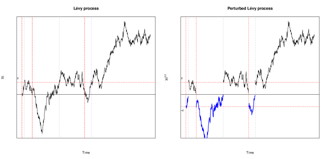
Figure 1: Left: Sample path of $X$. Right: Sample path of the perturbed process $X^{(\varepsilon)}$. The red vertical lines correspond to the sequence of stopping times $\{\rho_{k,\varepsilon}^{-},k\geq 1\}$, whereas the grey vertical lines correspond to $\{\rho_{k,\varepsilon}^{+},k\geq 1\}$.

It is straightforward from the definition of $X^{(\varepsilon)}$ that $X_{t}-\varepsilon\leq X_{t}^{(\varepsilon)}\leq X_{t}$, and that $X^{(\varepsilon)}\uparrow X$ uniformly when $\varepsilon\downarrow 0$, i.e.,

$$\lim_{\varepsilon\downarrow 0}\sup_{t\geq 0}|X_{t}^{(\varepsilon)}-X_{t}|=0.$$

In addition, we define the last zero process $g_{\varepsilon,t}$ associated to the process $X^{(\varepsilon)}$, that is,

$$g_{\varepsilon,t}=\sup\{0\leq s\leq t:X_{s}^{(\varepsilon)}\leq 0\}$$

for $\varepsilon>0$ and $t\geq 0$. The inequality $g_{t}\leq g_{\varepsilon,t}\leq g_{t}^{(\varepsilon)}$ holds for all $t\geq 0$. Taking $\varepsilon\downarrow 0$, and by the right continuity of $x\mapsto g_{t}^{(x)}$, we obtain that $g_{\varepsilon,t}\downarrow g_{t}$ when $\varepsilon\downarrow 0$ for all $t\geq 0$. Therefore, we have that $t-g_{\varepsilon,t}=:U_{\varepsilon,t}\uparrow U_{t}$ when $\varepsilon\downarrow 0$ for all $t\geq 0$.

Recall that the local time at zero, $L=\{L_{t},t\geq 0\}$, is a continuous process defined in terms of the Itô–Tanaka formula (see Protter, (2005) Chapter IV) and its measure $\textup{d}L_{t}$ is carried by the set $\{s\geq 0:X_{s-}=X_{s}=0\}$. Note that (see e.g. Corollary 3 in Protter, (2005) on p. 219) we have that

$$L_{t}=\sigma^{2}\lim_{\varepsilon\rightarrow 0}\frac{1}{\varepsilon}\int_{0}^{t}\mathbb{I}_{\{0\leq X_{s}\leq\varepsilon\}}\textup{d}s,\qquad\mathbb{P}\text{-a.s.}$$

So then, $L_{t}=0$ $\mathbb{P}$-almost surely if $\sigma=0$. For each $\varepsilon>0$ and $t\geq 0$, we define

$$M_{t}^{(\varepsilon)}=\sum_{k=1}^{\infty}\mathbb{I}_{\{\rho_{k,\varepsilon}^{-}<t\}}.$$

Note that $M_{t}^{(\varepsilon)}-1$ is the number of downcrossings of the level zero at time $t\geq 0$ of the process $X_{t}^{(\varepsilon)}$. We simply denote $M^{(\varepsilon)}=\lim_{t\rightarrow\infty}M_{t}^{(\varepsilon)}$ for all $\varepsilon>0$. It turns out that $M_{t}^{(\varepsilon)}$ works as an approximation of the local time at zero in some sense. We have the following lemma. The proof follows an argument analogous to the one in Revuz and Yor, (1999) (see Exercise VI.1.19).

Lemma 5.1.

Suppose that $X$ is a spectrally negative Lévy process. Then for all $t\geq 0$,

$$\lim_{\varepsilon\downarrow 0}\varepsilon M_{t}^{(\varepsilon)}=\frac{1}{2}L_{t},\qquad\mathbb{P}\text{-a.s}.$$

Proof.

From the Meyer–Itô formula (see Protter, (2005) Theorem 70) we know that

$$X_{t}^{+}=X_{0}^{+}+\int_{(0,t]}\mathbb{I}_{\{X_{s-}>0\}}\textup{d}X_{s}+\int_{(0,t]}\int_{(-\infty,0)}(X_{s-}+y)^{-}\mathbb{I}_{\{X_{s-}>0\}}N(\textup{d}s\times\textup{d}y)+\frac{1}{2}L_{t},$$

where $x^{+}$ and $x^{-}$ are the positive and negative part, respectively, of $x$ defined by $x^{+}=\max\{x,0\}$ and $x^{-}=-\min\{x,0\}$. Hence, for $t\geq 0$ and $1\leq k\leq M_{t}^{(\varepsilon)}$ we get that

$$X_{\rho_{k,\varepsilon}^{+}\wedge t}^{+}-X_{\rho_{k,\varepsilon}^{-}}^{+} =\int_{(\rho_{k,\varepsilon}^{-},\rho_{k,\varepsilon}^{+}\wedge t]}\mathbb{I}_{\{X_{s-}>0\}}\textup{d}X_{s}+\int_{(\rho_{k,\varepsilon}^{-},\rho_{k,\varepsilon}^{+}\wedge t]}\int_{(-\infty,0)}(X_{s-}+y)^{-}\mathbb{I}_{\{X_{s-}>0\}}N(\textup{d}s\times\textup{d}y)$$

$$\qquad+\frac{1}{2}(L_{\rho_{k,\varepsilon}^{+}\wedge t}-L_{\rho_{k,\varepsilon}^{-}}).$$

From the definition of the stopping times $\rho_{k,\varepsilon}^{-}$, we have that $X_{r}>0$ when $r\in[\rho_{k,\varepsilon}^{+},\rho_{k+1,\varepsilon}^{-})$ for some $k\geq 1$, and, since $L$ is continuous and only charge points in the set of zeros of $X$, we have that $L_{\rho_{k,\varepsilon}^{+}}=L_{\rho_{k+1,\varepsilon}^{-}}$ and $L_{t\wedge\rho_{M_{t}^{(\varepsilon)},\varepsilon}^{+}}=L_{t}$. Using a telescopic sum and the fact that $X_{r-}^{(\varepsilon)}\leq 0$ if and only if $r\in(\rho_{k,\varepsilon}^{-},\rho_{k,\varepsilon}^{+}]$, for some $k\geq 1$, we have that

$$X_{t\wedge\rho_{M_{t}^{(\varepsilon)},\varepsilon}^{+}}^{+} -X_{\rho_{M_{t}^{(\varepsilon)},\varepsilon}^{-}}^{+}+\sum_{k=1}^{M_{t}^{(\varepsilon)}-1}(X_{\rho_{k,\varepsilon}^{+}}^{+}-X_{\rho_{k,\varepsilon}^{-}}^{+})$$

$$=\int_{(0,t]}\mathbb{I}_{\{X_{s-}^{(\varepsilon)}\leq 0\}}\mathbb{I}_{\{X_{s-}>0\}}\textup{d}X_{s}+\int_{(0,t]}\int_{(-\infty,0)}(X_{s-}+y)^{-}\mathbb{I}_{\{X_{s-}^{(\varepsilon)}\leq 0\}}\mathbb{I}_{\{X_{s-}>0\}}N(\textup{d}s\times\textup{d}y)+\frac{1}{2}L_{t}.$$

Thus, since $X_{\rho_{k,\varepsilon}^{-}}\leq 0$ and $X_{\rho_{k,\varepsilon}^{+}}=\varepsilon$ for all $k\geq 1$, we obtain

$$X_{t\wedge\rho_{M_{t}^{(\varepsilon)},\varepsilon}^{+}}^{+} +\varepsilon(M_{t}^{(\varepsilon)}-1)$$

$$=\int_{(0,t]}\mathbb{I}_{\{X_{s-}^{(\varepsilon)}\leq 0\}}\mathbb{I}_{\{X_{s-}>0\}}\textup{d}X_{s}+\int_{(0,t]}\int_{(-\infty,0)}(X_{s-}+y)^{-}\mathbb{I}_{\{X_{s-}^{(\varepsilon)}\leq 0\}}\mathbb{I}_{\{X_{s-}>0\}}N(\textup{d}s\times\textup{d}y)+\frac{1}{2}L_{t}.$$

Note that $0\leq X_{t\wedge\rho_{M_{t}^{(\varepsilon)},\varepsilon}^{+}}^{+}\leq\varepsilon$ and then $\lim_{\varepsilon\downarrow 0}X_{t\wedge\rho_{M_{t}^{(\varepsilon)},\varepsilon}^{+}}^{+}=0$. Moreover, from the dominated convergence theorem for stochastic integrals (see for example, Theorem 32 Chapter IV of Protter, (2005)), we have that the first term in the right-hand side of the equation above converges to $0$ uniformly on compacts in probability, that is, for all $t>0$,

$$\sup_{0\leq s\leq t}\left|\int_{(0,s]}\mathbb{I}_{\{X_{r-}^{(\varepsilon)}\leq 0\}}\mathbb{I}_{\{X_{r-}>0\}}\textup{d}X_{r}\right|$$

converges to $0$ in probability when $\varepsilon\downarrow 0$. Note that, for all $s\geq 0$, we have that $(X_{s-}+y)^{-}\mathbb{I}_{\{X_{s-}^{(\varepsilon)}\leq 0\}}\mathbb{I}_{\{X_{s-}>0\}}\leq(X_{s-}+y)^{-}\mathbb{I}_{\{X_{s-}>0\}}$. Hence,

$$\int_{(0,t]}\int_{(-\infty,0)}(X_{s-}+y)^{-}\mathbb{I}_{\{X_{s-}>0\}}N(\textup{d}s\times\textup{d}y)<\infty$$

for all $t\geq 0$. Then, by the dominated convergence theorem

$$\lim_{\varepsilon\downarrow 0}\int_{(0,t]}\int_{(-\infty,0)}(X_{s-}+y)^{-}\mathbb{I}_{\{X_{s-}^{(\varepsilon)}\leq 0\}}\mathbb{I}_{\{X_{s-}>0\}}N(\textup{d}s\times\textup{d}y)=0$$

for any $t\geq 0$. Thus, for fixed $t\geq 0$, we have that $\varepsilon M_{t}^{(\varepsilon)}$ converges to $L_{t}/2$ in probability when $\varepsilon\downarrow 0$. We know that there exists a decreasing sub-sequence $\{\varepsilon_{n},n\geq 1\}$ converging to $0$ such that $\lim_{n\rightarrow\infty}\varepsilon_{n}M_{t}^{(\varepsilon_{n})}=L_{t}/2$, $\mathbb{P}$-a.s. From the fact that $M_{t}^{(\varepsilon)}$ increases when $\varepsilon$ decreases, we have that for each $\varepsilon\in[\varepsilon_{n+1},\varepsilon_{n}]$,

$$\varepsilon_{n+1}M_{t}^{(\varepsilon_{n})}\leq\varepsilon M_{t}^{(\varepsilon)}\leq\varepsilon_{n}M_{t}^{(\varepsilon_{n+1})}.$$

Hence, we conclude that $\lim_{\varepsilon\downarrow 0}\varepsilon M_{t}^{(\varepsilon)}=L_{t}/2$ $\mathbb{P}$-a.s as claimed. ∎

Let $\textbf{e}_{p}$ be an independent exponential random variable with parameter $p\geq 0$ (here we understand $\textbf{e}_{0}=\infty$). In the following Lemma, we calculate explicitly the probability mass function of the random variable $M_{\textbf{e}_{p}}$.

Lemma 5.2.

Let $\varepsilon>0$ fixed. We have that the probability mass function of the random variable $M_{\textbf{e}_{p}}^{(\varepsilon)}$ is given by

$$\mathbb{P}_{x}(M_{\textbf{e}_{p}}^{(\varepsilon)}=n)=\left\{\begin{array}[]{lc}1-\mathcal{I}^{(p,0)}(\varepsilon)e^{-\Phi(p)(\varepsilon-x)},&n=1,\\ \mathcal{I}^{(p,0)}(\varepsilon)e^{-\Phi(p)(\varepsilon-x)}[\mathcal{I}^{(p,\Phi(p))}(\varepsilon)]^{n-2}[1-\mathcal{I}^{(p,\Phi(p))}(\varepsilon)],&n\geq 2,\end{array}\right.$$ (28)

for all $x<\varepsilon$.

Proof.

We calculate the probability of the event $\{M_{\textbf{e}_{p}}^{(\varepsilon)}\geq n\}$, for $n\geq 2$, which happens if and only if $\{\rho_{n,\varepsilon}^{-}<\textbf{e}_{p}\}$. For any $x<\varepsilon$, we first calculate

$$\mathbb{P}_{x}(M_{\textbf{e}_{p}}^{(\varepsilon)}\geq 2) =\mathbb{P}_{x}(\rho_{2,\varepsilon}^{-}<\textbf{e}_{p})$$

$$=\mathbb{E}_{x}(\mathbb{P}_{x}(\rho_{2,\varepsilon}^{-}<\textbf{e}_{p},\rho_{1,\varepsilon}^{+}<\textbf{e}_{p}|\mathcal{F}_{\rho_{1,\varepsilon}^{+}}))$$

$$=\mathbb{E}_{\varepsilon}(e^{-p\tau_{0}^{-}}\mathbb{I}_{\{\tau_{0}^{-}<\infty\}})\mathbb{E}_{x}(e^{-p\tau_{\varepsilon}^{+}}\mathbb{I}_{\{\tau_{\varepsilon}^{+}<\infty\}})$$

$$=\mathcal{I}^{(p,0)}(\varepsilon)e^{-\Phi(p)(\varepsilon-x)},$$

where the second last equality follows from the strong Markov property and the lack of memory property of the exponential distribution, and the last equality by equations (1) and (4). Similarly, for $n\geq 3$ and $x<\varepsilon$,

$$\mathbb{P}_{x}(M_{\textbf{e}_{p}}^{(\varepsilon)}\geq n) =\mathbb{P}_{x}(\rho_{n,\varepsilon}^{-}<\textbf{e}_{p})$$

$$=\mathbb{E}_{x}(\mathbb{P}_{x}(\rho_{n,\varepsilon}^{-}<\textbf{e}_{p},\rho_{n-1,\varepsilon}^{+}<\textbf{e}_{p}|\mathcal{F}_{\rho_{n-1,\varepsilon}^{+}}))$$

$$=\mathbb{E}_{\varepsilon}(e^{-p\tau_{0}^{-}}\mathbb{I}_{\{\tau_{0}^{-}<\infty\}})\mathbb{E}_{x}(e^{-p\rho_{n-1,\varepsilon}^{+}}\mathbb{I}_{\{\rho_{n-1,\varepsilon}^{+}<\infty\}})$$

$$=\mathcal{I}^{(p,0)}(\varepsilon)\mathbb{E}_{x}(e^{-p\rho_{n-1,\varepsilon}^{+}}\mathbb{I}_{\{\rho_{n-1,\varepsilon}^{+}<\infty\}}).$$ (29)

Applying the strong Markov property at the stopping time $\rho_{n-1,\varepsilon}^{-}$, we get

$$\mathbb{P}_{x}(M_{\textbf{e}_{p}}^{(\varepsilon)}\geq n) =\mathcal{I}^{(p,0)}(\varepsilon)\mathbb{E}_{x}(e^{-p\rho_{n-1,\varepsilon}^{+}}\mathbb{I}_{\{\rho_{n-1,\varepsilon}^{+}<\infty\}})$$

$$=\mathcal{I}^{(p,0)}(\varepsilon)\mathbb{E}_{x}(e^{-p\rho_{n-1,\varepsilon}^{-}}\mathbb{I}_{\{\rho_{n-1,\varepsilon}^{-}<\infty\}}\mathbb{E}_{X_{\rho_{n-1,\varepsilon}^{-}}}(e^{-p\tau_{\varepsilon}^{+}}\mathbb{I}_{\{\tau_{0}^{+}<\infty\}}))$$

$$=\mathcal{I}^{(p,0)}e^{-\Phi(p)\varepsilon}(\varepsilon)\mathbb{E}_{x}(e^{-p\rho_{n-1,\varepsilon}^{-}+\Phi(p)X_{\rho_{n-1,\varepsilon}^{-}}}\mathbb{I}_{\{\rho_{n-1,\varepsilon}^{-}<\infty\}}),$$

where the last equality follows from equation (1). We apply again the strong Markov property at $\rho_{n-2,\varepsilon}^{+}$, and we use the fact that $X_{\rho_{k,\varepsilon}^{+}}=\varepsilon$ on the event $\{0<\rho_{k,\varepsilon}^{+}<\infty\}$, for all $k\geq 2$, to deduce for all $n\geq 3$ that

$$\mathbb{P}_{x}(M_{\textbf{e}_{p}}^{(\varepsilon)}\geq n) =\mathcal{I}^{(p,0)}(\varepsilon)e^{-\Phi(p)\varepsilon}\mathbb{E}_{\varepsilon}(e^{-p\tau_{0}^{-}+\Phi(p)X_{\tau_{0}^{-}}}\mathbb{I}_{\{\tau_{0}^{-}<\infty\}})\mathbb{E}_{x}(e^{-p\rho_{n-2,\varepsilon}^{+}}\mathbb{I}_{\{\rho_{n-2,\varepsilon}^{+}<\infty\}})$$

$$=\mathcal{I}^{(p,\Phi(p))}(\varepsilon)\mathbb{P}_{x}(M_{\textbf{e}_{p}}^{(\varepsilon)}\geq n-1),$$

where last equality follows from equations (4) and (29). Then by an induction argument we get that for all $n\geq 2$ and $x<\varepsilon$

$$\mathbb{P}_{x}(M_{\textbf{e}_{p}}^{(\varepsilon)}\geq n) =\mathcal{I}^{(p,0)}(\varepsilon)e^{-\Phi(p)(\varepsilon-x)}[\mathcal{I}^{(p,\Phi(p))}(\varepsilon)]^{n-2}.$$ (30)

The result then follows. ∎

Remark 5.3.

For all $\varepsilon>0$ fixed, we can describe the paths of the process $\{g_{\varepsilon,t},t\geq 0\}$ in terms of the stopping times $\{(\rho_{k,\varepsilon}^{-},\rho_{k,\varepsilon}^{+}),k\geq 1\}$. When $X_{t}^{(\varepsilon)}\leq 0$ we have that $\rho_{k,\varepsilon}^{-}\leq t<\rho_{k,\varepsilon}^{+}$, for some $k\geq 1$, and then $g_{\varepsilon,t}=t$. Similarly, when $X_{t}^{(\varepsilon)}>0$, there exists $k\geq 1$ such that $\rho_{k,\varepsilon}^{+}\leq t<\rho_{k+1,\varepsilon}^{-}$, and hence, $g_{\varepsilon,t}=\rho_{k,\varepsilon}^{+}$. The reader can refer to Figure 1 for a graphical representation of this fact.

5.2 Proof of Theorem 3.3

Suppose that $X_{t}>0$ and choose $\varepsilon<X_{t}$. Then, there exists $k\geq 1$ such that $\rho_{k,\varepsilon}^{+}\leq t<\rho_{k+1,\varepsilon}^{-}$ and $M_{t}^{(\varepsilon)}=k$. Using a telescopic sum, we have that

$$F(g_{\varepsilon,t},t,X_{t}^{(\varepsilon)}) =F(g_{\varepsilon,0},0,X^{(\varepsilon)}_{0})+\sum_{k=1}^{M_{t}^{(\varepsilon)}}[F(g_{\varepsilon,(\rho_{k,\varepsilon}^{+})-},\rho_{k,\varepsilon}^{+},X^{(\varepsilon)}_{(\rho_{k,\varepsilon}^{+})-})-F(g_{\varepsilon,\rho_{k,\varepsilon}^{-}},\rho_{k,\varepsilon}^{-},X^{(\varepsilon)}_{\rho_{k,\varepsilon}^{-}})]$$

$$\qquad+\sum_{k=1}^{M_{t}^{(\varepsilon)}}[F(g_{\varepsilon,\rho_{k,\varepsilon}^{+}},\rho_{k,\varepsilon}^{+},X^{(\varepsilon)}_{\rho_{k,\varepsilon}^{+}})-F(g_{\varepsilon,(\rho_{k,\varepsilon}^{+})-},\rho_{k,\varepsilon}^{+},X^{(\varepsilon)}_{(\rho_{k,\varepsilon}^{+})-})]$$

$$\qquad+\sum_{k=1}^{M_{t}^{(\varepsilon)}-1}[F(g_{\varepsilon,(\rho_{k+1,\varepsilon}^{-})-},\rho_{k+1,\varepsilon}^{-},X^{(\varepsilon)}_{(\rho_{k+1,\varepsilon}^{-})-})-F(g_{\varepsilon,\rho_{k,\varepsilon}^{+}},\rho_{k,\varepsilon}^{+},X^{(\varepsilon)}_{\rho_{k,\varepsilon}^{+}})]$$

$$\qquad+\sum_{k=1}^{M_{t}^{(\varepsilon)}-1}[F(g_{\varepsilon,\rho_{k+1,\varepsilon}^{-}},\rho_{k+1,\varepsilon}^{-},X^{(\varepsilon)}_{\rho_{k+1,\varepsilon}^{-}})-F(g_{\varepsilon,(\rho_{k+1,\varepsilon}^{-})-},\rho_{k+1,\varepsilon}^{-},X^{(\varepsilon)}_{(\rho_{k+1,\varepsilon}^{-})-})]$$

$$\qquad+[F(g_{\varepsilon,t},t,X^{(\varepsilon)}_{t})-F(g_{\varepsilon,\rho_{M_{t}^{(\varepsilon)},\varepsilon}^{+}},\rho_{M_{t}^{(\varepsilon)},\varepsilon}^{+},X^{(\varepsilon)}_{\rho_{M_{t}^{(\varepsilon)},\varepsilon}^{+}})].$$

Note that $g_{\varepsilon,(\rho_{k+1,\varepsilon}^{-})^{-}}=\rho_{k,\varepsilon}^{+}$, $g_{\varepsilon,\rho_{k,\varepsilon}^{-}}=\rho_{k,\varepsilon}^{-}$ and $g_{\varepsilon,(\rho_{k,\varepsilon}^{+})^{-}}=g_{\varepsilon,\rho_{k,\varepsilon}^{+}}=\rho_{k,\varepsilon}^{+}$ for all $k\geq 1$. Thus,

$$F(g_{\varepsilon,t},t,X_{t}^{(\varepsilon)}) =F(g_{\varepsilon,0},0,X^{(\varepsilon)}_{0})+\sum_{k=1}^{M_{t}^{(\varepsilon)}}[F(\rho_{k,\varepsilon}^{+},\rho_{k,\varepsilon}^{+},X_{\rho_{k,\varepsilon}^{+}}-\varepsilon)-F(\rho_{k,\varepsilon}^{-},\rho_{k,\varepsilon}^{-},X_{\rho_{k,\varepsilon}^{-}}-\varepsilon)]$$

$$\qquad+\sum_{k=1}^{M_{t}^{(\varepsilon)}}[F(\rho_{k,\varepsilon}^{+},\rho_{k,\varepsilon}^{+},X_{\rho_{k,\varepsilon}^{+}})-F(\rho_{k,\varepsilon}^{+},\rho_{k,\varepsilon}^{+},X_{\rho_{k,\varepsilon}^{+}}-\varepsilon)]$$

$$\qquad+\sum_{k=1}^{M_{t}^{(\varepsilon)}-1}[F(\rho_{k,\varepsilon}^{+},\rho_{k+1,\varepsilon}^{-},X_{(\rho_{k+1,\varepsilon}^{-})^{-}})-F(\rho_{k,\varepsilon}^{+},\rho_{k,\varepsilon}^{+},X_{\rho_{k,\varepsilon}^{+}})]$$

$$\qquad+\sum_{k=1}^{M_{t}^{(\varepsilon)}-1}[F(\rho_{k+1,\varepsilon}^{-},\rho_{k+1,\varepsilon}^{-},X_{\rho_{k+1,\varepsilon}^{-}}-\varepsilon)-F(\rho_{k,\varepsilon}^{+},\rho_{k+1,\varepsilon}^{-},X_{(\rho_{k+1,\varepsilon}^{-})^{-}})]$$

$$\qquad+[F(\rho_{M_{t}^{(\varepsilon)},\varepsilon}^{+},t,X_{t})-F(\rho_{M_{t}^{(\varepsilon)},\varepsilon}^{+},\rho_{M_{t}^{(\varepsilon)},\varepsilon}^{+},X_{\rho_{M_{t}^{(\varepsilon)},\varepsilon}^{+}})],$$

where we also used that $X^{(\varepsilon)}_{s}=X_{s}$ when $s\in[\rho_{k,\varepsilon}^{+},\rho_{k+1,\varepsilon}^{-})$ and $X^{(\varepsilon)}_{s}=X_{s}-\varepsilon$ when $s\in[\rho_{k,\varepsilon}^{-},\rho_{k,\varepsilon}^{+})$ for $k\geq 1$. Applying Itô formula (see Theorem 71 on Protter, (2005)) on intervals of the form $(\rho_{k,\varepsilon}^{-},\rho_{k,\varepsilon}^{+}]$ we have that

$$\sum_{k=1}^{M_{t}^{(\varepsilon)}}[F(\rho_{k,\varepsilon}^{+},\rho_{k,\varepsilon}^{+},X_{\rho_{k,\varepsilon}^{+}}-\varepsilon)-F(\rho_{k,\varepsilon}^{-},\rho_{k,\varepsilon}^{-},X_{\rho_{k,\varepsilon}^{-}}-\varepsilon)]$$

$$=\sum_{k=1}^{M_{t}^{(\varepsilon)}}\left[\int_{\rho_{k,\varepsilon}^{-}}^{\rho_{k,\varepsilon}^{+}}\frac{\partial}{\partial t}F_{g}(s,X_{s}-\varepsilon)\textup{d}s+\frac{1}{2}\sigma^{2}\int_{\rho_{k,\varepsilon}^{-}}^{\rho_{k,\varepsilon}^{+}}\frac{\partial^{2}}{\partial x^{2}}F(s,s,X_{s}-\varepsilon)\textup{d}s+\int_{(\rho_{k,\varepsilon}^{-},\rho_{k,\varepsilon}^{+}]}\frac{\partial}{\partial x}F(s,s,X_{s-}-\varepsilon)\textup{d}X_{s}\right]$$

$$\qquad+\sum_{k=1}^{M_{t}^{(\varepsilon)}}\int_{(\rho_{k,\varepsilon}^{-},\rho_{k,\varepsilon}^{+}]}\int_{(-\infty,0)}\left(F(s,s,X_{s-}+y-\varepsilon)-F(s,s,X_{s-}-\varepsilon)-y\frac{\partial}{\partial x}F(s,s,X_{s-}-\varepsilon)\right)N(\textup{d}s\times\textup{d}y)$$

$$=\int_{0}^{t}\frac{\partial}{\partial t}F_{g}(s,X_{s}^{(\varepsilon)})\mathbb{I}_{\{X_{s}^{(\varepsilon)}\leq 0\}}\textup{d}s+\frac{1}{2}\sigma^{2}\int_{0}^{t}\frac{\partial^{2}}{\partial x^{2}}F(g_{\varepsilon,s},s,X_{s}^{(\varepsilon)})\mathbb{I}_{\{X_{s}^{(\varepsilon)}\leq 0\}}\textup{d}s$$

$$\qquad+\int_{[0,t]}\frac{\partial}{\partial x}F(g_{\varepsilon,s-},s,X_{s-}^{(\varepsilon)})\mathbb{I}_{\{X_{s}^{(\varepsilon)}\leq 0\}}\textup{d}X_{s}-\int_{[0,t]}y\frac{\partial}{\partial x}F(g_{\varepsilon,s-},s,X_{s-}^{(\varepsilon)})\mathbb{I}_{\{X_{s-}^{(\varepsilon)}>0\}}\mathbb{I}_{\{X_{s-}^{(\varepsilon)}+y<0\}}N(\textup{d}s\times\textup{d}y)$$

$$\qquad+\int_{[0,t]}\int_{(-\infty,0)}\left(F(g_{\varepsilon,s-},s,X_{s-}^{(\varepsilon)}+y)-F(g_{\varepsilon,s-},s,X_{s-}^{(\varepsilon)})-y\frac{\partial}{\partial x}F(g_{\varepsilon,s-},s,X_{s-}^{(\varepsilon)})\right)\mathbb{I}_{\{X_{s-}^{(\varepsilon)}\leq 0\}}N(\textup{d}s\times\textup{d}y),$$

where the last equality follows since $X_{s}^{(\varepsilon)}\leq 0$ if and only if $s\in[\rho_{k,\varepsilon}^{-},\rho_{k,\varepsilon}^{+})$, for some $k\geq 1$ (and hence $g_{\varepsilon,s}=s$), $X$ has a jump at time $s$ on the event $\{X_{s-}^{(\varepsilon)}>0\}\cap\{X_{s}^{(\varepsilon)}<0\}$, and there are no jumps at time $\rho_{k,\varepsilon}^{+}$, for all $k\geq 1$. Similarly, applying Itô formula on intervals of the form $(\rho_{k,\varepsilon}^{+},\rho_{k+1}^{-})$, for $k\geq 1$, from the fact that $X$ does not jump at time $\rho_{k,\varepsilon}^{+}$, and since $X_{s}^{(\varepsilon)}>0$ if and only if $s\in[\rho_{k,\varepsilon}^{+},\rho_{k+1,\varepsilon}^{-})$ (and hence $g_{\varepsilon,s}=g_{\varepsilon,s-}=\rho_{k,\varepsilon}^{+}$) we have that

$$\sum_{k=1}^{M_{t}^{(\varepsilon)}-1}[F(\rho_{k,\varepsilon}^{+},\rho_{k+1,\varepsilon}^{-},X_{(\rho_{k+1,\varepsilon}^{-})^{-}})-F(\rho_{k,\varepsilon}^{+},\rho_{k,\varepsilon}^{+},X_{\rho_{k,\varepsilon}^{+}})]+[F(\rho_{M_{t}^{(\varepsilon)},\varepsilon}^{+},t,X_{t})-F(\rho_{M_{t}^{(\varepsilon)},\varepsilon}^{+},\rho_{M_{t}^{(\varepsilon)},\varepsilon}^{+},X_{\rho_{M_{t}^{(\varepsilon)},\varepsilon}^{+}})]$$

$$=\int_{0}^{t}\frac{\partial}{\partial t}F(g_{\varepsilon,s},s,X_{s}^{(\varepsilon)})\mathbb{I}_{\{X_{s}^{(\varepsilon)}>0\}}\textup{d}s$$

$$\qquad+\frac{1}{2}\sigma^{2}\int_{0}^{t}\frac{\partial^{2}}{\partial x^{2}}F(g_{\varepsilon,s},s,X_{s}^{(\varepsilon)})\mathbb{I}_{\{X_{s}^{(\varepsilon)}>0\}}\textup{d}s+\int_{[0,t]}\frac{\partial}{\partial x}F(g_{\varepsilon,s-},s,X_{s-}^{(\varepsilon)})\mathbb{I}_{\{X_{s}^{(\varepsilon)}>0\}}\textup{d}X_{s}$$

$$\qquad+\int_{[0,t]}\int_{(-\infty,0)}\left(F(g_{\varepsilon,s-},s,X_{s-}^{(\varepsilon)}+y)-F(g_{\varepsilon,s-},s,X_{s-}^{(\varepsilon)})-y\frac{\partial}{\partial x}F(g_{\varepsilon,s-},s,X_{s-}^{(\varepsilon)})\right)\mathbb{I}_{\{X_{s}^{(\varepsilon)}>0\}}N(\textup{d}s\times\textup{d}y).$$

Hence, we obtain that

$$F(g_{\varepsilon,t},t,X_{t}^{(\varepsilon)})=F(g_{\varepsilon,0},0,X^{(\varepsilon)}_{0})+\int_{0}^{t}\frac{\partial}{\partial t}F_{g}(s,X_{s}^{(\varepsilon)})\mathbb{I}_{\{X_{s}^{(\varepsilon)}\leq 0\}}\textup{d}s$$

$$\qquad+\int_{0}^{t}\frac{\partial}{\partial t}F(g_{\varepsilon,s},s,X_{s}^{(\varepsilon)})\mathbb{I}_{\{X_{s}^{(\varepsilon)}>0\}}\textup{d}s+\frac{1}{2}\sigma^{2}\int_{0}^{t}\frac{\partial^{2}}{\partial x^{2}}F(g_{\varepsilon,s},s,X_{s}^{(\varepsilon)})\textup{d}s$$

$$\qquad+\int_{0}^{t}\frac{\partial}{\partial x}F(g_{\varepsilon,s-},s,X^{(\varepsilon)}_{s-})\textup{d}X_{s}-\int_{[0,t]}\int_{(-\infty,0)}y\frac{\partial}{\partial x}F(g_{\varepsilon,s-},s,X^{(\varepsilon)}_{s-})\mathbb{I}_{\{X_{s-}^{(\varepsilon)}>0\}}\mathbb{I}_{\{X_{s-}^{(\varepsilon)}+y<0\}}N(\textup{d}s\times\textup{d}y)$$

$$\qquad+\int_{[0,t]}\int_{(-\infty,0)}\left(F(g_{\varepsilon,s-},s,X_{s-}^{(\varepsilon)}+y)-F(g_{\varepsilon,s-},s,X_{s-}^{(\varepsilon)})-y\frac{\partial}{\partial x}F(g_{\varepsilon,s-},s,X_{s-}^{(\varepsilon)})\right)\mathbb{I}_{\{X_{s}^{(\varepsilon)}>0\}}N(\textup{d}s\times\textup{d}y)$$

$$\qquad+\int_{[0,t]}\int_{(-\infty,0)}\left(F(g_{\varepsilon,s-},s,X_{s-}^{(\varepsilon)}+y)-F(g_{\varepsilon,s-},s,X_{s-}^{(\varepsilon)})-y\frac{\partial}{\partial x}F(g_{\varepsilon,s-},s,X_{s-}^{(\varepsilon)})\right)\mathbb{I}_{\{X_{s-}^{(\varepsilon)}\leq 0\}}N(\textup{d}s\times\textup{d}y)$$

$$\qquad+\sum_{k=1}^{M_{t}^{(\varepsilon)}}[F(\rho_{k,\varepsilon}^{+},\rho_{k,\varepsilon}^{+},X_{\rho_{k,\varepsilon}^{+}})-F(\rho_{k,\varepsilon}^{+},\rho_{k,\varepsilon}^{+},X_{\rho_{k,\varepsilon}^{+}}-\varepsilon)]$$

$$\qquad+\sum_{k=1}^{M_{t}^{(\varepsilon)}-1}[F(\rho_{k+1,\varepsilon}^{-},\rho_{k+1,\varepsilon}^{-},X_{\rho_{k+1,\varepsilon}^{-}}-\varepsilon)-F(\rho_{k,\varepsilon}^{+},\rho_{k+1,\varepsilon}^{-},X_{(\rho_{k+1,\varepsilon}^{-})^{-}})].$$

Since $X_{\rho_{k,\varepsilon}^{+}}=\varepsilon$ and $X$ can cross below $0$ either by creeping or by a jump, we have that the last two terms in the expression above become

$$\sum_{k=1}^{M_{t}^{(\varepsilon)}} [F(\rho_{k,\varepsilon}^{+},\rho_{k,\varepsilon}^{+},\varepsilon)-F(\rho_{k,\varepsilon}^{+},\rho_{k,\varepsilon}^{+},0)+\sum_{k=1}^{M_{t}^{(\varepsilon)}-1}[F(\rho_{k+1,\varepsilon}^{-},\rho_{k+1,\varepsilon}^{-},X_{\rho_{k+1,\varepsilon}^{-}}-\varepsilon)-F(\rho_{k,\varepsilon}^{+},\rho_{k+1,\varepsilon}^{-},X_{(\rho_{k+1,\varepsilon}^{-})^{-}})]$$

$$=\sum_{k=1}^{M_{t}^{(\varepsilon)}-1}[F(\rho_{k+1,\varepsilon}^{+},\rho_{k+1,\varepsilon}^{+},\varepsilon)-F(\rho_{k+1,\varepsilon}^{+},\rho_{k+1,\varepsilon}^{+},0)]+F(\rho_{1,\varepsilon}^{+},\rho_{1,\varepsilon}^{+},\varepsilon)-F(\rho_{1,\varepsilon}^{+},\rho_{1,\varepsilon}^{+},0)$$

$$\qquad+\sum_{k=1}^{M_{t}^{(\varepsilon)}-1}[F(\rho_{k+1,\varepsilon}^{-},\rho_{k+1,\varepsilon}^{-},-\varepsilon)-F(\rho_{k+1,\varepsilon}^{-},\rho_{k+1,\varepsilon}^{-},0)]\mathbb{I}_{\{X_{\rho_{k+1,\varepsilon}^{-}}=0\}}$$

$$\qquad+\int_{[0,t]}\int_{(-\infty,0)}[F(s,s,X_{s-}+y-\varepsilon)-F(g_{\varepsilon,s-},s,X_{s-})]\mathbb{I}_{\{X_{s-}^{(\varepsilon)}>0\}}\mathbb{I}_{\{X_{s-}^{(\varepsilon)}+y\leq 0\}}N(\textup{d}s\times\textup{d}y),$$

where we used the assumption that $\lim_{h\downarrow 0}F(\gamma,t,h)=F(t,t,0)$ for all $0\leq\gamma\leq t$, when $\rho>0$, $F$ is continuous and that $X_{(\rho_{k+1,\varepsilon}^{-})^{-}}=0$ on the event of creeping. Without loss of generality assume that $\varepsilon<1$. By the mean value theorem we have that, for each $k\geq 1$, there exist $c_{1,k}\in(0,\varepsilon)$ and $c_{2,k}\in(-\varepsilon,0)$ such that

$$\left|\sum_{k=1}^{M_{t}^{(\varepsilon)}-1}[F(\rho_{k+1,\varepsilon}^{+},\rho_{k+1,\varepsilon}^{+},\varepsilon)-F(\rho_{k+1,\varepsilon}^{+},\rho_{k+1,\varepsilon}^{+},0)]\right.$$

$$\qquad+\left.\sum_{k=1}^{M_{t}^{(\varepsilon)}-1}[F(\rho_{k+1,\varepsilon}^{-},\rho_{k+1,\varepsilon}^{-},-\varepsilon)-F(\rho_{k+1,\varepsilon}^{-},\rho_{k+1,\varepsilon}^{-},0)]\mathbb{I}_{\{X_{\rho_{k+1,\varepsilon}^{-}}=0\}}\right|$$

$$\leq\sum_{k=1}^{M_{t}^{(\varepsilon)}-1}\left|\frac{\partial}{\partial x}F(\rho_{k,\varepsilon}^{+},\rho_{k,\varepsilon}^{+},c_{1,k})-\frac{\partial}{\partial x}F(\rho_{k+1,\varepsilon}^{-},\rho_{k+1,\varepsilon}^{-},c_{2,k})\mathbb{I}_{\{X_{\rho_{k+1,\varepsilon}^{-}}=0\}}\right|\varepsilon$$

$$\leq 2K_{t}\varepsilon(M_{t}^{(\varepsilon)}-1),$$

where we used the fact that $(t,x)\mapsto\frac{\partial}{\partial x}F(t,t,x)$ exists and it is continuous on $[0,\infty)\times(-\infty,0]$ and on $[0,\infty)\times[0,\infty)$, and then $(s,x)\mapsto|\frac{\partial}{\partial x}F(s,s,x)|$ is bounded in the set $[0,t]\times[-1,1]$ by a constant, namely $K_{t}>0$. Moreover, we know that $\varepsilon M_{t}^{(\varepsilon)}\rightarrow L_{t}/2$, $\mathbb{P}$-a.s. when $\varepsilon\downarrow 0$ (see Lemma 5.1). Recall that $L_{t}=0$ $\mathbb{P}$-a.s. when $\sigma=0$ and that we are assuming (14) when $\sigma>0$. Hence, due to the dominated convergence and the mean value theorem, we see that

$$\left|\sum_{k=1}^{M_{t}^{(\varepsilon)}-1}[F(\rho_{k,\varepsilon}^{+},\rho_{k,\varepsilon}^{+},\varepsilon)-F(\rho_{k,\varepsilon}^{+},\rho_{k,\varepsilon}^{+},0)]+[F(\rho_{k+1,\varepsilon}^{-},\rho_{k+1,\varepsilon}^{-},-\varepsilon)-F(\rho_{k+1,\varepsilon}^{-},\rho_{k+1,\varepsilon}^{-},0)]\mathbb{I}_{\{X_{\rho_{k+1,\varepsilon}^{-}}=0\}}\right|\xrightarrow[a.s.]{\varepsilon\downarrow 0}0.$$

Therefore, by the dominated convergence theorem for stochastic integrals, we deduce that

$$F(g_{t}, t,X_{t})=F(g_{0},0,X_{0})+\int_{0}^{t}\frac{\partial}{\partial t}F_{g}(s,X_{s})\mathbb{I}_{\{X_{s}\leq 0\}}\textup{d}s+\int_{0}^{t}\frac{\partial}{\partial t}F(g_{s},s,X_{s})\mathbb{I}_{\{X_{s}>0\}}\textup{d}s$$

$$+\int_{0}^{t}\frac{\partial}{\partial x}F(g_{s-},s,X_{s-})\textup{d}X_{s}+\frac{1}{2}\sigma^{2}\int_{0}^{t}\frac{\partial^{2}}{\partial x^{2}}F(g_{s},s,X_{s})\textup{d}s$$

$$+\int_{[0,t]}\int_{(-\infty,0)}\left(F(g_{s-},s,X_{s^{-}}+y)-F(g_{s-},s,X_{s^{-}})-y\frac{\partial}{\partial x}F(g_{s-},s,X_{s^{-}})\right)\mathbb{I}_{\{X_{s}>0\}}N(\textup{d}s\times\textup{d}y)$$

$$+\int_{[0,t]}\int_{(-\infty,0)}\left(F(g_{s-},s,X_{s-}+y)-F(g_{s-},s,X_{s-})-y\frac{\partial}{\partial x}F(g_{s-},s,X_{s-})\right)\mathbb{I}_{\{X_{s-}\leq 0\}}N(\textup{d}s\times\textup{d}y)$$

$$+\int_{[0,t]}\int_{(-\infty,0)}\left(F(s,s,X_{s-}+y)-F(g_{s-},s,X_{s-})-y\frac{\partial}{\partial x}F(g_{s-},s,X_{s-})\right)\mathbb{I}_{\{0<X_{s-}<-y\}}N(\textup{d}s\times\textup{d}y).$$ (31)

From the fact that $g_{t}$ is continuous in the set $\{t\geq 0:X_{t}>0\text{ or }X_{t-}\leq 0\}$, we obtain the desired result. The case when $X_{t}\leq 0$ is similar, and the proof is omitted.

5.3 Proof of Theorem 3.6

First, note that, since $|K(U_{s},X_{s})|\leq C(U_{s},X_{s})$ for all $s\geq 0$ and $\mathbb{E}_{u,x}\left(\int_{0}^{\infty}e^{-qr}C(U_{r},X_{r}+y)\textup{d}r\right)<\infty$ for all $(u,x)\in E$ and $y\in\mathbb{R}$, we have that $K^{+}$ and $K^{-}$ are finite. Moreover, since $u\mapsto C(u,x)$ is monotone for all $x\in\mathbb{R}$ and non-negative, we have that for all $r\geq 0$ and $\varepsilon>0$,

$$|K(U_{\varepsilon,r},X_{r}^{(\varepsilon)})|\leq C(U_{\varepsilon,r},X_{r}^{(\varepsilon)})\leq C(U_{r},X_{r})+C(U_{r},X_{r}-\varepsilon)+C(U_{r}^{(\varepsilon)},X_{r})+C(U_{r}^{(\varepsilon)},X_{r}-\varepsilon),$$

where $U_{r}^{(\varepsilon)}=r-g_{t}^{(\varepsilon)}=r-\sup\{0\leq s\leq r:X_{s}\leq\varepsilon\}$ and we used that $U_{t}\geq U_{\varepsilon,t}\geq U_{t}^{(\varepsilon)}$, for all $t\geq 0$. It follows from integrability of $e^{-qr}C(U_{r},X_{r}+y)$ with respect to the product measure $\mathbb{P}_{u,x}\times\textup{d}r$, for all $(u,x)\in E$, by dominated convergence theorem and left-continuity in each argument of $K$ that for $x\leq 0$,

$$\mathbb{E}_{x}\left(\int_{0}^{\infty}e^{-qr}K(U_{r},X_{r})\textup{d}r\right)=\lim_{\varepsilon\downarrow 0}\mathbb{E}_{x}\left(\int_{0}^{\infty}e^{-qr}K(U_{\varepsilon,r},X_{r}^{(\varepsilon)})\textup{d}r\right).$$

Then we calculate the right-hand side of the equation above. Fix $\varepsilon>0$, using the fact that $\{M^{(\varepsilon)}=n\}=\{\rho_{n,\varepsilon}^{-}<\infty\}\cap\{\rho_{n+1,\varepsilon}^{-}=\infty\}$ for $n\geq 1$, we have for any $x\leq 0$ that

$$\mathbb{E}_{x}\left(\int_{0}^{\infty}e^{-qr}K(U_{\varepsilon,r},X_{r}^{(\varepsilon)})\textup{d}r\right) =\sum_{n=1}^{\infty}\mathbb{E}_{x}\left(\mathbb{I}_{\{M^{(\varepsilon)}=n\}}\int_{0}^{\infty}e^{-qr}K(U_{\varepsilon,r},X_{r}^{(\varepsilon)})\textup{d}r\right)$$

$$=\sum_{n=1}^{\infty}\sum_{k=1}^{n}\mathbb{E}_{x}\left(\mathbb{I}_{\{\rho_{n,\varepsilon}^{-}<\infty\}}\mathbb{I}_{\{\rho_{n+1,\varepsilon}^{-}=\infty\}}\int_{\rho_{k,\varepsilon}^{-}}^{\rho_{k,\varepsilon}^{+}}e^{-qr}K(0,X_{r}^{(\varepsilon)})\textup{d}r\right)$$

$$\qquad+\sum_{n=2}^{\infty}\sum_{k=1}^{n-1}\mathbb{E}_{x}\left(\mathbb{I}_{\{\rho_{n,\varepsilon}^{-}<\infty\}}\mathbb{I}_{\{\rho_{n+1,\varepsilon}^{-}=\infty\}}\int_{\rho_{k,\varepsilon}^{+}}^{\rho_{k+1,\varepsilon}^{-}}e^{-qr}K(r-\rho_{k,\varepsilon}^{+},X_{r}^{(\varepsilon)})\textup{d}r\right)$$

$$\qquad+\sum_{n=1}^{\infty}\mathbb{E}_{x}\left(\mathbb{I}_{\{\rho_{n,\varepsilon}^{+}<\infty\}}\mathbb{I}_{\{\rho_{n+1,\varepsilon}^{-}=\infty\}}\int_{\rho_{n,\varepsilon}^{+}}^{\rho_{n+1,\varepsilon}^{-}}e^{-qr}K(r-\rho_{n,\varepsilon}^{+},X_{r}^{(\varepsilon)})\textup{d}r\right),$$

where the last equality follows from the fact that $g_{\varepsilon,r}=r$ when $r\in[\rho_{k,\varepsilon}^{-},\rho_{k,\varepsilon}^{+}]$ and $g_{\varepsilon,r}=\rho_{k,\varepsilon}^{+}$ when $r\in[\rho_{k,\varepsilon}^{+},\rho_{k+1,\varepsilon}^{-})$, for some $k\geq 1$. We first analyse the first double sum on the right-hand side of the expression above. Conditioning with respect to the filtration at the stopping time $\rho_{k,\varepsilon}^{+}$, the strong Markov property and the fact that $X$ creeps upwards we get

$$\sum_{n=1}^{\infty} \sum_{k=1}^{n}\mathbb{E}_{x}\left(\mathbb{I}_{\{\rho_{n,\varepsilon}^{-}<\infty\}}\mathbb{I}_{\{\rho_{n+1,\varepsilon}^{-}=\infty\}}\int_{\rho_{k,\varepsilon}^{-}}^{\rho_{k,\varepsilon}^{+}}e^{-qr}K(0,X_{r}^{(\varepsilon)})\textup{d}r\right)$$

$$=K^{-}(x-\varepsilon)+\sum_{n=3}^{\infty}\sum_{k=2}^{n-1}\mathbb{E}_{x}\left(\mathbb{I}_{\{\rho_{k,\varepsilon}^{+}<\infty\}}\int_{\rho_{k,\varepsilon}^{-}}^{\rho_{k,\varepsilon}^{+}}e^{-qr}K(0,X_{r}-\varepsilon)\textup{d}r\right)\mathbb{P}_{\varepsilon}(M^{(\varepsilon)}=n-k+1)$$

$$\qquad+\sum_{n=2}^{\infty}\mathbb{E}_{x}\left(\mathbb{I}_{\{\rho_{n,\varepsilon}^{-}<\infty\}}\mathbb{I}_{\{\rho_{n,\varepsilon}^{+}=\infty\}}\int_{\rho_{n,\varepsilon}^{-}}^{\rho_{n,\varepsilon}^{+}}e^{-qr}K(0,X_{r}-\varepsilon)\textup{d}r\right)$$

$$\qquad+\sum_{n=2}^{\infty}\mathbb{E}_{x}\left(\mathbb{I}_{\{\rho_{n,\varepsilon}^{+}<\infty\}}\int_{\rho_{n,\varepsilon}^{-}}^{\rho_{n,\varepsilon}^{+}}e^{-qr}K(0,X_{r}-\varepsilon)\textup{d}r\right)\mathbb{P}_{\varepsilon}(M^{(\varepsilon)}=1),$$

where the first term in the last equality corresponds to the first excursion of $X^{(\varepsilon)}$ below zero (case $k=1$) and we used the fact that $X_{r}^{(\varepsilon)}=X_{r}-\varepsilon$ for $r\in[\rho_{k,\varepsilon}^{-},\rho_{k,\varepsilon}^{+}]$ for any $k\geq 1$. For $x\in\mathbb{R}$, we define the auxiliary functions

$$K_{1}^{-}(x) :=\mathbb{E}_{x}\left(\mathbb{I}_{\{\tau_{0}^{+}<\infty\}}\int_{0}^{\tau_{0}^{+}}e^{-qr}K(0,X_{r})\textup{d}r\right),$$

$$K_{2}^{-}(x) :=\mathbb{E}_{x}\left(\mathbb{I}_{\{\tau_{0}^{+}=\infty\}}\int_{0}^{\tau_{0}^{+}}e^{-qr}K(0,X_{r})\textup{d}r\right).$$

Then we have that $K^{-}(x)=K_{1}^{-}(x)+K_{2}^{-}(x)$ for all $x\in\mathbb{R}$. Conditioning with respect to the filtration at time $\rho_{k,\varepsilon}^{-}$ (resp. $\rho_{n,\varepsilon}^{-}$), we obtain that

$$\sum_{n=1}^{\infty}\sum_{k=1}^{n}\mathbb{E}_{x}\left(\mathbb{I}_{\{\rho_{n,\varepsilon}^{-}<\infty\}}\mathbb{I}_{\{\rho_{n+1,\varepsilon}^{-}=\infty\}}\int_{\rho_{k,\varepsilon}^{-}}^{\rho_{k,\varepsilon}^{+}}e^{-qr}K(0,X_{r}^{(\varepsilon)})\textup{d}r\right)$$

$$=K^{-}(x-\varepsilon)+\sum_{n=3}^{\infty}\sum_{k=2}^{n-1}\mathbb{E}_{x}\left(\mathbb{I}_{\{\rho_{k,\varepsilon}^{-}<\infty\}}e^{-q\rho_{k,\varepsilon}^{-}}K_{1}^{-}(X_{\rho_{k,\varepsilon}^{-}}-\varepsilon)\right)\mathbb{P}_{\varepsilon}(M^{(\varepsilon)}=n-k+1)$$

$$\qquad+\sum_{n=2}^{\infty}\mathbb{E}_{x}\left(\mathbb{I}_{\{\rho_{n,\varepsilon}^{-}<\infty\}}e^{-q\rho_{n,\varepsilon}^{-}}K_{2}^{-}(X_{\rho_{k,\varepsilon}^{-}}-\varepsilon)\right)+\sum_{n=2}^{\infty}\mathbb{E}_{x}\left(\mathbb{I}_{\{\rho_{n,\varepsilon}^{-}<\infty\}}e^{-q\rho_{n,\varepsilon}^{-}}K_{1}^{-}(X_{\rho_{k,\varepsilon}^{-}}-\varepsilon)\right)\mathbb{P}_{\varepsilon}(M^{(\varepsilon)}=1)$$

$$=K^{-}(x-\varepsilon)+\sum_{n=3}^{\infty}\sum_{k=2}^{n-1}\mathbb{E}_{\varepsilon}(\mathbb{I}_{\{\tau_{0}^{-}<\infty\}}e^{-q\tau_{0}^{-}}K_{1}^{-}(X_{\tau_{0}^{-}}-\varepsilon))\mathbb{E}_{x}\left(\mathbb{I}_{\{\rho_{k-1,\varepsilon}^{+}<\infty\}}e^{-q\rho_{k-1,\varepsilon}^{+}}\right)\mathbb{P}_{\varepsilon}(M^{(\varepsilon)}=n-k+1)$$

$$\qquad+\sum_{n=2}^{\infty}\mathbb{E}_{\varepsilon}\left(\mathbb{I}_{\{\tau_{0}^{-}<\infty\}}e^{-q\tau_{0}^{-}}K_{2}^{-}(X_{\tau_{0}^{-}}-\varepsilon)\right)\mathbb{E}_{x}\left(\mathbb{I}_{\{\rho_{n-1,\varepsilon}^{+}<\infty\}}e^{-q\rho_{n-1,\varepsilon}^{+}}\right)$$

$$\qquad+\sum_{n=2}^{\infty}\mathbb{E}_{\varepsilon}\left(\mathbb{I}_{\{\tau_{0}^{-}<\infty\}}e^{-q\tau_{0}^{-}}K_{1}^{-}(X_{\tau_{0}^{-}}-\varepsilon)\right)\mathbb{E}_{x}\left(\mathbb{I}_{\{\rho_{n-1,\varepsilon}^{+}<\infty\}}e^{-q\rho_{n-1,\varepsilon}^{+}}\right)\mathbb{P}_{\varepsilon}(M^{(\varepsilon)}=1)$$

$$=K^{-}(x-\varepsilon)+\sum_{n=3}^{\infty}\sum_{k=2}^{n-1}\mathbb{E}_{\varepsilon}(\mathbb{I}_{\{\tau_{0}^{-}<\infty\}}e^{-q\tau_{0}^{-}}K_{1}^{-}(X_{\tau_{0}^{-}}-\varepsilon))\frac{\mathbb{P}_{x}(M_{\textbf{e}_{q}}^{(\varepsilon)}\geq k)}{\mathcal{I}^{(q,0)}(\varepsilon)}\mathbb{P}_{\varepsilon}(M^{(\varepsilon)}=n-k+1)$$

$$\qquad+\sum_{n=2}^{\infty}\mathbb{E}_{\varepsilon}\left(\mathbb{I}_{\{\tau_{0}^{-}<\infty\}}e^{-q\tau_{0}^{-}}K_{2}^{-}(X_{\tau_{0}^{-}}-\varepsilon)\right)\frac{\mathbb{P}_{x}(M_{\textbf{e}_{q}}^{(\varepsilon)}\geq n)}{\mathcal{I}^{(q,0)}(\varepsilon)}$$

$$\qquad+\sum_{n=2}^{\infty}\mathbb{E}_{\varepsilon}\left(\mathbb{I}_{\{\tau_{0}^{-}<\infty\}}e^{-q\tau_{0}^{-}}K_{1}^{-}(X_{\tau_{0}^{-}}-\varepsilon)\right)\frac{\mathbb{P}_{x}(M_{\textbf{e}_{q}}^{(\varepsilon)}\geq n)}{\mathcal{I}^{(q,0)}(\varepsilon)}\mathbb{P}_{\varepsilon}(M^{(\varepsilon)}=1),$$

where the second equality follows from conditioning with respect to time $\rho_{k-1,\varepsilon}^{+}$ (resp. $\rho_{n-1,\varepsilon}^{+}$) and the Markov property of $X$, and the last equality from equation (29). From Lemma 5.2 and solving the corresponding geometric series, we get

$$\sum_{n=1}^{\infty} \sum_{k=1}^{n}\mathbb{E}_{x}\left(\mathbb{I}_{\{\rho_{n,\varepsilon}^{-}<\infty\}}\mathbb{I}_{\{\rho_{n+1,\varepsilon}^{-}=\infty\}}\int_{\rho_{k,\varepsilon}^{-}}^{\rho_{k,\varepsilon}^{+}}e^{-qr}K(0,X_{r}^{(\varepsilon)})\textup{d}r\right)$$

$$=K^{-}(x-\varepsilon)+\mathbb{E}_{\varepsilon}\left(\mathbb{I}_{\{\tau_{0}^{-}<\infty\}}e^{-q\tau_{0}^{-}}K^{-}(X_{\tau_{0}^{-}}-\varepsilon)\right)\frac{e^{-\Phi(q)(\varepsilon-x)}}{1-\mathcal{I}^{(q,\Phi(q))}(\varepsilon)}.$$

Similarly, from the strong Markov property, the fact that $X$ creeps upwards, equation (4) and Lemma 5.2, we can see that

$$\sum_{n=2}^{\infty} \sum_{k=1}^{n-1}\mathbb{E}_{x}\left(\mathbb{I}_{\{\rho_{n,\varepsilon}^{-}<\infty\}}\mathbb{I}_{\{\rho_{n+1,\varepsilon}^{-}=\infty\}}\int_{\rho_{k,\varepsilon}^{+}}^{\rho_{k+1,\varepsilon}^{-}}e^{-qr}K(r-\rho_{k,\varepsilon}^{+},X_{r}^{(\varepsilon)})\textup{d}r\right)$$

$$\qquad+\sum_{n=1}^{\infty}\mathbb{E}_{x}\left(\mathbb{I}_{\{\rho_{n,\varepsilon}^{+}<\infty\}}\mathbb{I}_{\{\rho_{n+1,\varepsilon}^{-}=\infty\}}\int_{\rho_{n,\varepsilon}^{+}}^{\rho_{n+1,\varepsilon}^{-}}e^{-qr}K(r-\rho_{n,\varepsilon}^{+},X_{r}^{(\varepsilon)})\textup{d}r\right)$$

$$=K^{+}(0,\varepsilon)\frac{e^{-\Phi(q)(\varepsilon-x)}}{1-\mathcal{I}^{(q,\Phi(q))}(\varepsilon)}.$$

Therefore, by the dominated convergence theorem we have that for all $x\leq 0$,

$$\mathbb{E}_{x} \left(\int_{0}^{\infty}e^{-qr}K(U_{r},X_{r})\textup{d}r\right)$$

$$=\lim_{\varepsilon\downarrow 0}\left\{K^{-}(x-\varepsilon)+\frac{e^{-\Phi(q)(\varepsilon-x)}}{1-\mathcal{I}^{(q,\Phi(q))}(\varepsilon)}\left[\mathbb{E}_{\varepsilon}\left(\mathbb{I}_{\{\tau_{0}^{-}<\infty\}}e^{-q\tau_{0}^{-}}K^{-}(X_{\tau_{0}^{-}}-\varepsilon)\right)+K^{+}(0,\varepsilon)\right]\right\}.$$

When $u,x>0$ we deduce that,

$$\mathbb{E}_{u,x} \left(\int_{0}^{\infty}e^{-qr}K(U_{r},X_{r})\textup{d}r\right)$$

$$=\mathbb{E}_{x}\left(\int_{0}^{\tau_{0}^{-}}e^{-qr}K(u+r,X_{r})\textup{d}r\right)+\mathbb{E}_{x}\left(\mathbb{I}_{\{\tau_{0}^{-}<\infty\}}\int_{\tau_{0}^{-}}^{\infty}e^{-qr}K(U_{r},X_{r})\textup{d}r\right)$$

$$=K^{+}(u,x)+\lim_{\varepsilon\downarrow 0}\mathbb{E}_{x}\left(\mathbb{I}_{\{\tau_{0}^{-}<\infty\}}e^{-q\tau_{0}^{-}}K^{-}(X_{\tau_{0}^{-}}-\varepsilon)\right)$$

$$\qquad+e^{\Phi(q)x}\mathcal{I}^{(q,\Phi(q))}(x)\lim_{\varepsilon\downarrow 0}\frac{e^{-\Phi(q)\varepsilon}}{1-\mathcal{I}^{(q,\Phi(q))}(\varepsilon)}\left[\mathbb{E}_{\varepsilon}\left(\mathbb{I}_{\{\tau_{0}^{-}<\infty\}}e^{-q\tau_{0}^{-}}K^{-}(X_{\tau_{0}^{-}}-\varepsilon)\right)+K^{+}(0,\varepsilon)\right],$$ (32)

where the last equality follows from conditioning at time $\tau_{0}^{-}$, the strong Markov property and equation (4). Using Fubini’s theorem and equation (9) we have that for all $x<0$,

$$K^{-}(x)=\int_{(-\infty,0)}K(0,y)\int_{0}^{\infty}e^{-qr}\mathbb{P}_{x}(X_{r}\in\textup{d}y,r<\tau_{0}^{+})\textup{d}r=\int_{-\infty}^{0}K(0,y)[e^{\Phi(q)x}W^{(q)}(-y)-W^{(q)}(x-y)]\textup{d}y.$$

Then, for any $x>0$ and $\varepsilon>0$, we deduce from Fubini’s theorem and equation (4) that

$$\mathbb{E}_{x}\left(\mathbb{I}_{\{\tau_{0}^{-}<\infty\}}e^{-q\tau_{0}^{-}}K^{-}(X_{\tau_{0}^{-}}-\varepsilon)\right)$$

$$=e^{\Phi(q)(x-\varepsilon)}\mathcal{I}^{(q,\Phi(q))}(x)\int_{-\varepsilon}^{0}K(0,y)W^{(q)}(-y)\textup{d}y$$

$$\qquad+\int_{-\infty}^{-\varepsilon}K(0,y)\left[e^{\Phi(q)(x-\varepsilon)}\mathcal{I}^{(q,\Phi(q))}(x)W^{(q)}(-y)-\mathbb{E}_{x}\left(\mathbb{I}_{\{\tau_{0}^{-}<\infty\}}e^{-q\tau_{0}^{-}}W^{(q)}(X_{\tau_{0}^{-}}-\varepsilon-y)\right)\right]\textup{d}y.$$

Let $x,\varepsilon>0$ and $y<-\varepsilon$. From the monotone convergence theorem and (3) we have that

$$\mathbb{E}_{x} \left(\mathbb{I}_{\{\tau_{0}^{-}<\infty\}}e^{-q\tau_{0}^{-}}W^{(q)}(X_{\tau_{0}^{-}}-\varepsilon-y)\right)$$

$$=\lim_{a\rightarrow\infty}\mathbb{E}_{x}\left(\mathbb{I}_{\{\tau_{0}^{-}<\tau_{a}^{+}\}}e^{-q\tau_{0}^{-}}W^{(q)}(X_{\tau_{0}^{-}}-\varepsilon-y)\right)$$

$$=\lim_{a\rightarrow\infty}\mathbb{E}_{x}\left(e^{-q\tau_{0}^{-}\wedge\tau_{a}^{+}}W^{(q)}(X_{\tau_{0}^{-}\wedge\tau_{a}^{+}}-\varepsilon-y)\right)-\lim_{a\rightarrow\infty}\mathbb{E}_{x}\left(\mathbb{I}_{\{\tau_{a}^{+}<\tau_{0}^{-}\}}e^{-q\tau_{a}^{+}}W^{(q)}(a-\varepsilon-y)\right)$$

$$=\lim_{a\rightarrow\infty}\mathbb{E}_{x-\varepsilon-y}\left(e^{-q\tau_{-\varepsilon-y}^{-}\wedge\tau_{a-\varepsilon-y}^{+}}W^{(q)}(X_{\tau_{-\varepsilon-y}^{-}\wedge\tau_{a-\varepsilon-y}^{+}})\right)-\lim_{a\rightarrow\infty}W^{(q)}(a-\varepsilon-y)\frac{W^{(q)}(x)}{W^{(q)}(a)}$$

$$=W^{(q)}(x-\varepsilon-y)-e^{-\Phi(q)(\varepsilon+y)}W^{(q)}(x),$$

where the last equality follows since, for any $a\geq 0$, the process $e^{-q(t\wedge\tau_{0}^{-}\wedge\tau_{a}^{+})}W^{(q)}(X_{t\wedge\tau_{0}^{-}\wedge\tau_{a}^{+}})$ is a martingale, the optional sampling theorem (note that $\tau_{-\varepsilon-y}^{-}\leq\tau_{0}^{-}$) and since $\lim_{a\rightarrow\infty}W^{(q)}(a-z)/W^{(q)}(a)=e^{-\Phi(q)z}$ for $z\leq a$ and $a\geq 0$ (see Exercises 8.5 and 8.12 in Kyprianou, (2014)). Hence, we obtain that for any $x>0$,

$$\mathbb{E}_{x}\left(\mathbb{I}_{\{\tau_{0}^{-}<\infty\}}e^{-q\tau_{0}^{-}}K^{-}(X_{\tau_{0}^{-}}-\varepsilon)\right)$$

$$=e^{\Phi(q)(x-\varepsilon)}\mathcal{I}^{(q,\Phi(q))}(x)\int_{-\varepsilon}^{0}K(0,y)W^{(q)}(-y)\textup{d}y$$

$$\qquad+\int_{-\infty}^{-\varepsilon}K(0,y)\left[e^{\Phi(q)(x-\varepsilon)}\mathcal{I}^{(q,\Phi(q))}(x)W^{(q)}(-y)-W^{(q)}(x-\varepsilon-y)+e^{-\Phi(q)(\varepsilon+y)}W^{(q)}(x)\right]\textup{d}y.$$

Substituting the expression above in (5.3) and taking $\varepsilon\downarrow 0$ we obtain that for all $u,x>0$,

$$\mathbb{E}_{u,x}\left(\int_{0}^{\infty}e^{-qr}K(U_{r},X_{r})\textup{d}r\right) =K^{+}(u,x)+\int_{-\infty}^{0}K(0,y)\left[e^{\Phi(q)(x-y)}\Phi^{\prime}(q)-W^{(q)}(x-y)\right]\textup{d}y$$

$$\qquad+e^{\Phi(q)x}\left[1-\psi^{\prime}(\Phi(q)+)e^{-\Phi(q)x}W^{(q)}(x)\right]\lim_{\varepsilon\downarrow 0}\frac{K^{+}(0,\varepsilon)}{\psi^{\prime}(\Phi(q)+)W^{(q)}(\varepsilon)}.$$

The proof is now complete.

5.4 Proof of Theorem 4.1

We first state a verification Lemma that provides sufficient conditions for the optimality of a given candidate solution $\tau^{*}$.

Lemma 5.4.

Suppose that $\tau^{*}$ is candidate solution to the optimal stopping problem and let $V^{*}$ its corresponding value function, i.e., $V^{*}(u,x)=\mathbb{E}_{x,u}\left(\int_{0}^{\tau^{*}}e^{-rs}G(U_{s},X_{s})\textup{d}s\right)$. Assume that

1. $V^{*}(u,x)\geq 0$ for all $(u,x)\in E$.

2. For each $(u,x)\in E$ and $N>0$, the stochastic process $\{Z_{t\wedge\tau_{N}^{+}},t\geq 0\}$ is a supermartingale under the measure $\mathbb{P}_{u,x}$, where

   $$Z_{t}=e^{-rt}V^{*}(U_{t},X_{t})+\int_{0}^{t}e^{-rs}G(U_{s},X_{s})\textup{d}s.$$

Then $V=V^{*}$ and the stopping time $\tau^{*}$ is an optimal stopping time for (21).

Proof.

From the definition of $V$ we deduce that $V\geq V^{*}$. On the other hand, due to the optimal sampling theorem we have that, for any $t\geq 0$, $N>0$ and any stopping time $\tau\in\mathcal{T}$, the stopped process $Z_{t\wedge\tau\wedge\tau_{N}^{+}}$ is a supermartingale. This implies that for any $t\geq 0$, $N>0$ and $\tau\in\mathcal{T}$,

$$V^{*}(u,x)\geq\mathbb{E}_{u,x}\left(e^{-r(T\wedge\tau)}V^{*}(U_{T\wedge\tau},X_{T\wedge\tau})+\int_{0}^{T\wedge\tau}e^{-rs}G(U_{s},X_{s})\textup{d}s\right)\geq\mathbb{E}_{u,x}\left(\int_{0}^{T\wedge\tau}e^{-rs}G(U_{s},X_{s})\textup{d}s\right),$$

where $T=t\wedge\tau_{N}^{+}$ and the last inequality follows since $V^{*}\geq 0$, by assumption. From the dominated convergence theorem we conclude (see (20)), by taking $t,N\rightarrow\infty$ in the equation above, that

$$V^{*}(u,x)\geq\mathbb{E}_{u,x}\left(\int_{0}^{\tau}e^{-rs}G(U_{s},X_{s})\textup{d}s\right)$$

for all $(u,x)\in E$ and $\tau\in\mathcal{T}$. Hence, we have that $V\leq V^{*}$, implying that $V=V^{*}$. Therefore, the supremum in (21) is attained by $\tau^{*}$ as claimed. ∎

For $z\leq 0$ fixed, we define the function

$$V_{z}(u,x):=\mathbb{E}_{x,u}\left(\int_{0}^{\tau_{z}^{-}}e^{-rs}G(U_{s},X_{s})\textup{d}s\right),$$

for $(u,x)\in E$. The following lemma gives a semi-explicit expression for $V_{z}$ in terms of the scale functions.

Lemma 5.5.

For any $z<0$ and $(u,x)\in E$ such that $x\geq z$ we have that

$$V_{z}(u,x) =K^{+}(u,x)+\left[e^{\Phi(r)z}W^{(r)}(x-z)-W^{(r)}(x)\right]\int_{(0,\infty)}\int_{0}^{\infty}G(v,y)\frac{y}{v}e^{-rv}\mathbb{P}(X_{v}\in\textup{d}y)\textup{d}v$$

$$\qquad+e^{\Phi(r)z}W^{(r)}(x-z)\int_{z}^{0}G(0,y)e^{-\Phi(r)y}\textup{d}y-\int_{z}^{0}G(0,y)W^{(r)}(x-y)\textup{d}y.$$ (33)

Proof.

Note that for any $(u,x)\in E$,

$$V_{z}(u,x)=\mathbb{E}_{x,u}\left(\int_{0}^{\tau_{z}^{-}}e^{-rs}G(U_{s},X_{s})\mathbb{I}_{\{X_{s}>0\}}\textup{d}s\right)+\mathbb{E}_{x}\left(\int_{0}^{\tau_{z}^{-}}e^{-rs}G(0,X_{s})\mathbb{I}_{\{X_{s}\leq 0\}}\textup{d}s\right),$$

where the two terms on the right-hand side above are finite due to equation (20). Using equation (10) and Fubini’s theorem we deduce that for any $x\geq z$,

$$\mathbb{E}_{x}\left(\int_{0}^{\tau_{z}^{-}}e^{-rs}G(0,X_{s})\mathbb{I}_{\{X_{s}\leq 0\}}\textup{d}s\right) =\mathbb{E}_{x-z}\left(\int_{0}^{\tau_{0}^{-}}e^{-rs}G(0,X_{s}+z)\mathbb{I}_{\{X_{s}+z\leq 0\}}\textup{d}s\right)$$

$$=\int_{(0,-z]}G(0,y+z)\int_{0}^{\infty}e^{-rs}\mathbb{P}_{x-z}\left(X_{s}\in\textup{d}y,s<\tau_{0}^{-}\right)\textup{d}s$$

$$=\int_{0}^{-z}G(0,y+z)\left[e^{-\Phi(r)y}W^{(r)}(x-z)-W^{(r)}(x-z-y)\right]\textup{d}y$$

$$=e^{\Phi(r)z}W^{(r)}(x-z)\int_{z}^{0}G(0,y)e^{-\Phi(r)y}\textup{d}y-\int_{z}^{0}G(0,y)W^{(r)}(x-y)\textup{d}y.$$

On the other hand, from the strong Markov property, we have that for $(u,x)\in E$ such that $x\geq z$,

$$\mathbb{E}_{x,u}\left(\int_{0}^{\tau_{z}^{-}}e^{-rs}G(U_{s},X_{s})\mathbb{I}_{\{X_{s}>0\}}\textup{d}s\right) =H(u,x)-\mathbb{E}_{x}(e^{-r\tau_{z}^{-}}\mathbb{I}_{\{\tau_{z}^{-}<\infty\}}H(0,X_{\tau_{z}^{-}})),$$

where

$$H(u,x) :=\mathbb{E}_{u,x}\left(\int_{0}^{\infty}e^{-rs}G(U_{s},X_{s})\mathbb{I}_{\{X_{s}>0\}}\textup{d}s\right).$$ (34)

It follows from (20) that $|H(u,x)|<\infty$ for all $(u,x)\in E$. Hence, by using the potential measure of $(U,X)$ given in Corollary 3.10 we see that for any $(u,x)\in E$,

$$H(u,x) =\int_{(0,\infty)}\int_{0}^{\infty}G(v,y)\int_{0}^{\infty}e^{-rs}\mathbb{P}_{u,x}(X_{s}\in\textup{d}y,U_{s}\in\textup{d}v)\textup{d}s$$

$$=\int_{(0,\infty)}\int_{u}^{\infty}G(v,y)e^{-r(v-u)}\mathbb{P}_{x}(X_{v-u}\in\textup{d}y,v-u<\tau_{0}^{-})\textup{d}v$$

$$\qquad+\left[e^{\Phi(r)x}\Phi^{\prime}(r)-W^{(r)}(x)\right]\int_{(0,\infty)}\int_{0}^{\infty}G(v,y)\frac{y}{v}e^{-rv}\mathbb{P}(X_{v}\in\textup{d}y)\textup{d}v$$

$$=K^{+}(u,x)+\left[e^{\Phi(r)x}\Phi^{\prime}(r)-W^{(r)}(x)\right]\int_{(0,\infty)}\int_{0}^{\infty}G(v,y)\frac{y}{v}e^{-rv}\mathbb{P}(X_{v}\in\textup{d}y)\textup{d}v.$$ (35)

So that, by using (4), we deduce that for any $x\in\mathbb{R}$,

$$\mathbb{E}_{x}(e^{-r\tau_{z}^{-}}\mathbb{I}_{\{\tau_{z}^{-}<\infty\}}H(0,X_{\tau_{z}^{-}})) =\Phi^{\prime}(r)\mathbb{E}_{x}\left(e^{-r\tau_{z}^{-}+\Phi(r)X_{\tau_{z}^{-}}}\mathbb{I}_{\{\tau_{z}^{-}<\infty\}}\right)\int_{(0,\infty)}\int_{0}^{\infty}G(v,y)\frac{y}{v}e^{-rv}\mathbb{P}(X_{v}\in\textup{d}y)\textup{d}v$$

$$=\left(\Phi^{\prime}(r)e^{\Phi(r)x}-e^{\Phi(r)z}W^{(r)}(x-z)\right)\int_{(0,\infty)}\int_{0}^{\infty}G(v,y)\frac{y}{v}e^{-rv}\mathbb{P}(X_{v}\in\textup{d}y)\textup{d}v.$$ (36)

Therefore, we get that

$$\mathbb{E}_{x,u} \left(\int_{0}^{\tau_{z}^{-}}e^{-rs}G(U_{s},X_{s})\mathbb{I}_{\{X_{s}>0\}}\textup{d}s\right)$$

$$=H(u,x)-\mathbb{E}_{x}(e^{-r\tau_{z}^{-}}\mathbb{I}_{\{\tau_{z}^{-}<\infty\}}H(0,X_{\tau_{z}^{-}}))$$

$$=K^{+}(u,x)+\left[e^{\Phi(r)z}W^{(r)}(x-z)-W^{(r)}(x)\right]\int_{(0,\infty)}\int_{0}^{\infty}G(v,y)\frac{y}{v}e^{-rv}\mathbb{P}(X_{v}\in\textup{d}y)\textup{d}v$$

for any $(u,x)\in E$. The result follows. ∎

It is common for optimal stopping problems to choose candidate solutions to satisfy the principle of smooth fit. Recall that we are assuming that $\sigma>0$ so that, in this case, $W^{(r)}$ is $C^{2}$ on $(0,\infty)$ with $W^{(r)\prime}(0+)=2/\sigma^{2}$ (see e.g. Theorem 3.10 and Lemma 3.2 Kyprianou et al., (2011)). Then, by differentiating $V_{z}(u,x)$ with respect to $x$, we obtain for $z<x<0$ that,

$$\frac{\partial}{\partial x}V_{z}(0,x) =e^{\Phi(r)z}W^{(r)\prime}(x-z)\left[\int_{(0,\infty)}\int_{0}^{\infty}G(v,y)\frac{y}{v}e^{-rv}\mathbb{P}(X_{v}\in\textup{d}y)\textup{d}v+\int_{z}^{0}G(0,y)e^{-\Phi(r)y}\textup{d}y\right]$$

$$\qquad-\int_{z}^{x}G(0,y)W^{(r)\prime}(x-y)\textup{d}y.$$

Then, by letting $x\downarrow z$, we see that the equation

$$\frac{\partial}{\partial x}V_{z}(0,z-)=0$$

is satisfied if and only if $z$ is solution to the equation

$$\int_{(0,\infty)}\int_{0}^{\infty}G(v,y)\frac{y}{v}e^{-rv}\mathbb{P}(X_{v}\in\textup{d}y)\textup{d}v+\int_{z}^{0}G(0,y)e^{-\Phi(r)y}=0.$$

That is, if $z=z^{*}$. In the next lemma we verify that the characterization of $z^{*}$ given in the statement of Theorem 4.1 indeed holds and that condition i) given in Lemma 5.4 holds when $z\geq z^{*}$.

Lemma 5.6.

For $z\leq 0$, we define the function

$$f(z)=\int_{(0,\infty)}\int_{0}^{\infty}G(v,y)\frac{y}{v}e^{-rv}\mathbb{P}(X_{v}\in\textup{d}y)\textup{d}v+\int_{z}^{0}G(0,y)e^{-\Phi(r)y}\textup{d}y.$$

Then the equation $f(z)=0$ has a unique solution $z^{*}$ on $(-\infty,0)$ such that $z^{*}\leq y_{0}$. Moreover, we have that $V_{z}(u,x)\geq 0$ for all $z\geq z^{*}$ and $(u,x)\in E$.

Proof.

From Corollary 3.10 and by assumption (20) we know that

$$0\leq f(0)=\int_{(0,\infty)}\int_{0}^{\infty}G(v,y)\frac{y}{v}e^{-rv}\mathbb{P}(X_{v}\in\textup{d}y)\textup{d}v=\frac{1}{\Phi^{\prime}(r)}\mathbb{E}\left(\int_{0}^{\infty}e^{-rs}G(U_{s},X_{s})\mathbb{I}_{\{X_{s}>0\}}\textup{d}s\right)<\infty.$$

On the other hand, since $G(0,y)$ is non positive on $(-\infty,y_{0})$, we have that $f(z)$ is increasing on $(-\infty,y_{0})$ with $f(z)>0$ for all $y_{0}\leq z\leq 0$ and $\lim_{y\rightarrow-\infty}f(z)=-\infty$, where the latter follows due to the assumption $\lim_{y\rightarrow-\infty}G(0,y)<0$. Then, due to the continuity of $f$, we see that the equation $f(z)=0$ has a unique solution $z^{*}$ on $(-\infty,y_{0})$.

Next, we proceed to show the statement on $V_{z}$. Since $G(u,x)$ is non negative for all $(u,x)\in E$ such that $x\geq y_{0}$, we see that $V_{z}(x,u)\geq 0$ for all $(u,x)\in E$ and $z\geq y_{0}$. Take $z<0$ and $(u,x)\in E$ such that $x>z$, we see from (33) that

$$\frac{\partial}{\partial z}V_{z}(u,x)=f(z)\frac{\partial}{\partial z}(e^{\Phi(r)z}W^{(r)}(x-z)).$$

Note that we can write $e^{\Phi(r)z}W^{(r)}(x-z)=e^{\Phi(r)x}W_{\Phi(r)}(x-z)$, where $W_{\Phi(0)}$ is the $0$-scale function under the measure $\mathbb{P}^{\Phi(0)}$ (see e.g. the proof of Theorem 8.1 in Kyprianou, (2014)). Then we see that the mapping $z\mapsto e^{\Phi(r)z}W^{(r)}(x-z)$ is non increasing on $\mathbb{R}$, and then, $\frac{\partial}{\partial z}V_{z}(u,x)\leq 0$ for all $(u,x)\in E$ and $z^{*}\leq z<0$ such that $x>z$. We conclude that, for $(u,x)\in E$ fixed such that $x>z^{*}$, the mapping $z\mapsto V_{z}(x,u)$ is non increasing on $[z^{*},x\wedge 0)$. Hence,

$$V_{z}(x,u)\geq\lim_{z\uparrow x\wedge 0}V_{z}(u,x)\geq 0$$

for any $z^{*}\leq z\leq 0$ and $(u,x)\in E$ such that $x>z$. The proof is now complete. ∎

For ease of notation we denote $V^{*}=V_{z^{*}}$. Note that for any $(u,x)\in E$,

$$V^{*}(u,x)=K^{+}(u,x)-W^{(r)}(x)\int_{(0,\infty)}\int_{0}^{\infty}G(v,y)\frac{y}{v}e^{-rv}\mathbb{P}(X_{v}\in\textup{d}y)\textup{d}v-\int_{z^{*}}^{0}G(0,y)W^{(r)}(x-y)\textup{d}y.$$ (37)

Next, we show that the supermartingale property holds for $V^{*}$.

Lemma 5.7.

For any $N>0$ we have that the process $\{Z_{t\wedge\tau_{N}^{+}}^{*},t\geq 0\}$ is a supermartingale under $\mathbb{P}_{u,x}$, for each $(u,x)\in E$, where

$$Z_{t}^{*}=e^{-rt}V^{*}(U_{t},X_{t})+\int_{0}^{t}e^{-rs}G(U_{s},X_{s})\textup{d}s.$$

Proof.

Due to the fact that $X$ is of infinite variation, we have that $\mathbb{P}(\tau_{0}^{-}=0)=1$ and $W^{(r)}$ is continuous on $\mathbb{R}$. Thus, $V_{z}$ is continuous on $E$ and $\lim_{h\downarrow 0}V^{*}(u,h)=V^{*}(0,0)$ for any $u\geq 0$. Moreover, since we are assuming that $\rho>0$, we have that $W^{(r)}\in C^{2}(0,\infty)$ with $W^{(r)\prime}(0+)=2/\sigma^{2}$ (see Lemma 3.2 and Theorem 3.10 in Kyprianou et al., (2011)). Hence, we have that $V_{z}(u,x)$ is $C^{1,1}$ function on $[0,\infty)\times[0,\infty)$ and the second derivative $\frac{\partial^{2}}{\partial x^{2}}V^{*}(u,x)$ exists on $(0,\infty)$ for all $u\geq 0$ (recall that we are assuming that $K^{+}$ is $C^{1,2}$ function on $[0,\infty)\times[0,\infty)$). On the other hand, for $z^{*}<x<0$ we have that

$$\frac{\partial}{\partial x}V^{*}(0,x) =\int_{z^{*}}^{x}G(0,y)W^{(r)\prime}(x-y)\textup{d}y,$$ (38)

$$\frac{\partial^{2}}{\partial x^{2}}V^{*}(0,x) =\int_{z^{*}}^{x}G(0,y)W^{(r)\prime\prime}(x-y)\textup{d}y+G(0,x)W^{(r)\prime}(0+).$$ (39)

Hence, we see that $V_{z}$ is $C^{1}$ function on $(-\infty,0]$ and its second derivative exists on $(-\infty,0]\setminus\{z^{*}\}$. Furthermore, by applying formula (3.6) to $H(0,0)$ (see equation (34)) and from (35) we see that

$$\Phi^{\prime}(r)\int_{(0,\infty)}\int_{0}^{\infty}G(v,y)e^{-rv}\frac{y}{v}\mathbb{P}(X_{v}\in\textup{d}y)\textup{d}v=H(0,0)=\lim_{\varepsilon\downarrow 0}\frac{K^{+}(0,\varepsilon)}{\psi^{\prime}(\Phi(r))W^{(r)}(\varepsilon)}=\Phi^{\prime}(r)\frac{\sigma^{2}}{2}\frac{\partial}{\partial x}K^{+}(0,0+).$$ (40)

Hence, from the equality above and (37) we deduce that

$$\frac{\partial}{\partial x}V^{*}(0,0+)=\frac{\partial}{\partial x}V^{*}(0,0-).$$

It can be easily seen that the process $\{Z_{t\wedge\tau_{z^{*}}^{-}}^{*},t\geq 0\}$ is a martingale. Hence, by using standard arguments (cf. Peskir and Shiryaev, (2006), Section III.7.2 or Lamberton and Mikou, (2008), Proposition 2.4), we deduce that

$$\mathcal{A}_{U,X}(V^{*})(u,x)+G=rV^{*}$$ (41)

for all $(u,x)\in E$ such that $x\geq z^{*}$, where from Corollary 3.5 we obtain that

$$\mathcal{A}_{(U,X)}(V^{*})(u,x) =\frac{\partial}{\partial u}V^{*}(u,x)\mathbb{I}_{\{x>0\}}-\mu\frac{\partial}{\partial x}V^{*}(u,x)+\frac{1}{2}\sigma^{2}\frac{\partial^{2}}{\partial x^{2}}V^{*}(u,x)$$

$$\qquad+\int_{(-\infty,0)}\left(V^{*}(u,x+y)-V^{*}(u,x)-y\mathbb{I}_{\{y>-1\}}\frac{\partial}{\partial x}V^{*}(u,x)\right)\mathbb{I}_{\{x+y>0\}}\Pi(\textup{d}y)$$

$$\qquad+\int_{(-\infty,0)}\left(V^{*}(0,x+y)-V^{*}(0,x)-y\mathbb{I}_{\{y>-1\}}\frac{\partial}{\partial x}V^{*}(0,x)\right)\mathbb{I}_{\{x\leq 0\}}\Pi(\textup{d}y)$$

$$\qquad+\int_{(-\infty,0)}\left(V^{*}(0,x+y)-V^{*}(0,x)-y\mathbb{I}_{\{y>-1\}}\frac{\partial}{\partial x}V^{*}(u,x)\right)\mathbb{I}_{\{x>0\}}\mathbb{I}_{\{x+y<0\}}\Pi(\textup{d}y).$$

Hence, for any $(u,x)\in E$, $t\geq 0$ and $N>0$, by applying the version of Itô formula derived in Theorem 3.3 and letting $T=t\wedge\tau_{N}^{+}$, we deduce that, under $\mathbb{P}_{u,x}$,

$$e^{-rT} V^{*}(U_{T},X_{T})$$

$$=V^{*}(u,x)-\int_{0}^{T}e^{-rs}rV^{*}(U_{s},X_{s})\textup{d}s+\int_{0}^{T}e^{-rs}\frac{\partial}{\partial u}V^{*}(U_{s},X_{s})\mathbb{I}_{\{X_{s}>0\}}\textup{d}s$$

$$\qquad+\int_{0}^{T}e^{-rs}\frac{\partial}{\partial x}V^{*}(U_{s-},X_{s-})\textup{d}X_{s}+\frac{1}{2}\sigma^{2}\int_{0}^{T}e^{-rs}\frac{\partial^{2}}{\partial x^{2}}V^{*}(U_{s},X_{s})\textup{d}s$$

$$\qquad+\int_{[0,T]}e^{-rs}\int_{(-\infty,0)}\left(V^{*}(U_{s},X_{s^{-}}+y)-V^{*}(U_{s-},X_{s-})-y\frac{\partial}{\partial x}V^{*}(U_{s-},X_{s-})\right)N(\textup{d}s\times\textup{d}y)$$

$$=M_{T}-\int_{0}^{T}e^{-rs}[\mathcal{A}_{(U,X)}(V^{*})(U_{s},X_{s})-rV^{*}(U_{s},X_{s})]\textup{d}s$$

$$=M_{T}-\int_{0}^{T}e^{-rs}G(U_{s},X_{s})\mathbb{I}_{\{X_{s}>z^{*}\}}\textup{d}s,$$

where $\{M_{t\wedge\tau_{N}^{+}},t\geq 0\}$ is a martingale and the last equality follows since $V^{*}(0,x)=0$ for all $x\leq z^{*}$ and then $\mathcal{A}_{U,X}(V^{*})(0,x)=0$ for all $x\leq z^{*}$. Hence, we deduce that, for each $t\geq 0$ and $N>0$,

$$Z^{*}_{t\wedge\tau_{N}^{+}}=e^{-r(t\wedge\tau_{N}^{+})}V^{*}(U_{t\wedge\tau_{N}^{+}},X_{t\wedge\tau_{N}^{+}})+\int_{0}^{t\wedge\tau_{N}^{+}}e^{-rs}G(U_{s},X_{s})\textup{d}s=M_{t\wedge\tau_{N}^{+}}+\int_{0}^{t\wedge\tau_{N}^{+}}e^{-rs}G(0,X_{s})\mathbb{I}_{\{X_{s}\leq z^{*}\}}\textup{d}s.$$

Hence, since $G(0,x)\leq 0$ for all $x\leq z^{*}\leq y_{0}$, we conclude that $\{Z_{t\wedge\tau_{N}^{+}}^{*},t\geq 0\}$ is a supermartingale as claimed. ∎

Then the statements in Theorem 4.1 follow from Lemmas 5.4, 5.6 and 5.7. Finally, note from (38) that the smooth fit property holds in this case.

References

- Alili and Kyprianou, (2005) Alili, L. and Kyprianou, A. E. (2005). Some remarks on first passage of Lévy processes, the American put and pasting principles. The Annals of Applied Probability, 15(3):2062–2080.
- Avram et al., (2004) Avram, F., Kyprianou, A. E., and Pistorius, M. R. (2004). Exit problems for spectrally negative Lévy processes and applications to (Canadized) Russian options. The Annals of Applied Probability, 14(1):215–238.
- Azéma and Yor, (1989) Azéma, J. and Yor, M. (1989). Étude d’une martingale remarquable. Séminaire de probabilités de Strasbourg, 23:88–130.
- Baurdoux, (2009) Baurdoux, E. J. (2009). Last exit before an exponential time for spectrally negative Lévy processes. Journal of Applied Probability, 46(2):542–558.
- Baurdoux et al., (2016) Baurdoux, E. J., Kyprianou, A. E., and Ott, C. (2016). Optimal prediction for positive self-similar Markov processes. Electron. J. Probab., 21:24 pp.
- (6) Baurdoux, E. J. and Pedraza, J. M. (2020a). optimal prediction of the last zero of a spectrally negative Lévy process.
- (7) Baurdoux, E. J. and Pedraza, J. M. (2020b). Predicting the last zero of a spectrally negative Lévy process. In XIII Symposium on Probability and Stochastic Processes, pages 77–105. Springer.
- Baurdoux and Van Schaik, (2014) Baurdoux, E. J. and Van Schaik, K. (2014). Predicting the time at which a Lévy process attains its ultimate supremum. Acta applicandae mathematicae, 134(1):21–44.
- Bertoin, (1998) Bertoin, J. (1998). Lévy processes, volume 121. Cambridge university press.
- Bichteler, (2002) Bichteler, K. (2002). Stochastic integration with jumps. Encyclopedia of Mathematics and its Applications. Cambridge University Press.
- Bingham, (1975) Bingham, N. H. (1975). Fluctuation theory in continuous time. Advances in Applied Probability, 7(4):705–766.
- Chan, (2004) Chan, T. (2004). Some Applications of Lévy Process in insurance and finance. Finance, 25:71–94.
- Chiu and Yin, (2005) Chiu, S. N. and Yin, C. (2005). Passage times for a spectrally negative Lévy process with applications to risk theory. Bernoulli, 11(3):511–522.
- Cont and Tankov, (2003) Cont, R. and Tankov, P. (2003). Financial modelling with jump processes. Chapman and Hall/CRC.
- Dassios and Wu, (2011) Dassios, A. and Wu, S. (2011). Double-barrier Parisian options. J. Appl. Probab., 48(1):1–20.
- du Toit and Peskir, (2008) du Toit, J. and Peskir, G. (2008). Predicting the time of the ultimate maximum for Brownian motion with drift. In Mathematical Control Theory and Finance, pages 95–112. Springer Berlin Heidelberg.
- du Toit et al., (2008) du Toit, J., Peskir, G., and Shiryaev, A. N. (2008). Predicting the last zero of Brownian motion with drift. Stochastics, 80(2-3):229–245.
- Dynkin, (1965) Dynkin, E. B. (1965). Markov processes, Vols. I, II. Springer-Verlag Berlin Heidelberg.
- Glover and Hulley, (2014) Glover, K. and Hulley, H. (2014). Optimal prediction of the last-passage time of a transient diffusion. SIAM Journal on Control and Optimization, 52(6):3833–3853.
- Glover et al., (2013) Glover, K., Hulley, H., and Peskir, G. (2013). Three-dimensional Brownian motion and the golden ratio rule. Ann. Appl. Probab., 23(3):895–922.
- (21) Huzak, M., Perman, M., Šikić, H., and Vondraček, Z. (2004a). Ruin probabilities and decompositions for general perturbed risk processes. The Annals of Applied Probability, 14(3):1378–1397.
- (22) Huzak, M., Perman, M., Šikić, H., and Vondraček, Z. (2004b). Ruin probabilities for competing claim processes. Journal of applied probability, 41(3):679–690.
- Jacka, (1991) Jacka, S. D. (1991). Optimal stopping and the American put. Mathematical Finance, 1(2):1–14.
- Klüppelberg et al., (2004) Klüppelberg, C., Kyprianou, A. E., and Maller, R. A. (2004). Ruin probabilities and overshoots for general Lévy insurance risk processes. The Annals of Applied Probability, 14(4):1766–1801.
- Kyprianou et al., (2011) Kyprianou, A., Kuznetsov, A., and Rivero, V. (2011). The theory of scale functions for spectrally negative Lévy processes. Lévy Matters, Springer Lecture Notes in Mathematics.
- Kyprianou et al., (2006) Kyprianou, A., Schoutens, W., and Wilmott, P. (2006). Exotic option pricing and advanced Lévy models. John Wiley & Sons.
- Kyprianou and Surya, (2005) Kyprianou, A. and Surya, B. (2005). On the Novikov-Shiryaev optimal stopping problems in continuous time. Electronic Communications in Probability, 10:146–154.
- Kyprianou, (2014) Kyprianou, A. E. (2014). Fluctuations of Lévy processes with applications. Springer Berlin Heidelberg.
- Kyprianou and Surya, (2007) Kyprianou, A. E. and Surya, B. A. (2007). A note on a change of variable formula with local time-space for Lévy processes of bounded variation. In Séminaire de Probabilités XL, pages 97–104. Springer.
- Lamberton and Mikou, (2008) Lamberton, D. and Mikou, M. (2008). The critical price for the American put in an exponential Lévy model. Finance and Stochastics, 12(4):561–581.
- Leland, (1994) Leland, H. E. (1994). Corporate debt value, bond covenants, and optimal capital structure. The journal of finance, 49(4):1213–1252.
- Manso et al., (2010) Manso, G., Strulovici, B., and Tchistyi, A. (2010). Performance-sensitive debt. The Review of Financial Studies, 23(5):1819–1854.
- Mordecki, (1999) Mordecki, E. (1999). Optimal stopping for a diffusion with jumps. Finance and Stochastics, 3(2):227–236.
- Mordecki, (2002) Mordecki, E. (2002). Optimal stopping and perpetual options for Lévy processes. Finance and Stochastics, 6(4):473–493.
- Paroissin and Rabehasaina, (2013) Paroissin, C. and Rabehasaina, L. (2013). First and last passage times of spectrally positive Lévy processes with application to reliability. Methodology and Computing in Applied Probability, 17(2):351–372.
- Peskir, (2007) Peskir, G. (2007). A change-of-variable formula with local time on surfaces. In Séminaire de probabilités XL, pages 70–96. Springer.
- Peskir and Shiryaev, (2006) Peskir, G. and Shiryaev, A. (2006). Optimal stopping and free-boundary problems. Birkhäuser Basel.
- Protter, (2005) Protter, P. E. (2005). Stochastic integration and differential equations. Springer Berlin Heidelberg.
- Quah and Strulovici, (2013) Quah, J. K.-H. and Strulovici, B. (2013). Discounting, values, and decisions. Journal of Political Economy, 121(5):896–939.
- Revuz and Yor, (1999) Revuz, D. and Yor, M. (1999). Continuous martingales and Brownian motion. Springer Berlin Heidelberg.
- Salminen, (1988) Salminen, P. (1988). On the first hitting time and the last exit time for a Brownian motion to/from a moving boundary. Advances in Applied Probability, 20(2):411–426.
- Sato, (1999) Sato, K.-i. (1999). Lévy processes and infinitely divisible distributions. Cambridge university press.
- Schoutens, (2003) Schoutens, W. (2003). Lévy processes in finance: pricing financial derivatives. Wiley Online Library.
- Shiryaev, (2009) Shiryaev, A. N. (2009). On conditional-extremal problems of the quickest detection of nonpredictable times of the observable Brownian motion. Theory of Probability & Its Applications, 53(4):663–678.