Diffusion properties of self-propelled particles in cellular flows

Abstract

We study the dynamics of a self-propelled particle advected by a steady laminar flow. The persistent motion of the self-propelled particle is described by an active Ornstein-Uhlenbeck process. We focus on the diffusivity properties of the particle as a function of persistence time and free-diffusion coefficient, revealing non-monotonic behaviors, with the occurrence of a minimum and steep growth in the regime of large persistence time. In the latter limit, we obtain an analytical prediction for the scaling of the diffusion coefficient with the parameters of the active force. Our study sheds light on the effect of an inhomogeneous environment on the diffusion of active particles, such as living microorganisms and motile phytoplankton in fluids.

I Introduction

In recent years, great interest has been raised by the complex dynamics of biological microorganisms or artificial microswimmers, which convert energy from the environment into systematic motion Bechinger et al. (2016); Marchetti et al. (2013). Nowadays, these non-equilibrium systems are classified as self-propelled particles (SPP), a subclass of dry active matter. The behavior of SPP without environmental constraints has been largely studied and has shown a very fascinating phenomenology, such as: swarming, clustering Buttinoni et al. (2013); Palacci et al. (2013); Ginot et al. (2018), phase-separation Fily and Marchetti (2012); Bialké et al. (2015); Cates and Tailleur (2015); Digregorio et al. (2018); Solon et al. (2018); Chiarantoni et al. (2020), spontaneous velocity alignments Caprini et al. (2020); Lam et al. (2015); Ginelli et al. (2010) and vortex formation Sumino et al. (2012). These phenomena have not a passive Brownian counterpart, because of the intrinsic non-equilibrium nature of the self-propelled motion, characterized by a persistence time $\tau$, and, in particular, due to the peculiar interplay between active forces and interactions among particles. Even in non-interacting cases, the diffusive properties of SPP have been a matter of intense study both experimentally and numerically since the self-propulsion enhances the diffusivity with respect to any passive tracers ten Hagen et al. (2011); Sevilla and Nava (2014); Basu et al. (2018); Scholz et al. (2018); Sevilla and Castro-Villarreal (2019); Caprini and Marconi (2019).

The dynamics of SPP in complex and non-homogeneous environments constitute a central issue for its great biological interest. Indeed, in Nature, microswimmers or bacteria, when encounter soft or solid obstacles Miño et al. (2018) or even hard walls Li and Tang (2009), accumulate in front of them producing interesting patterns Wensink and Löwen (2008); Elgeti and Gompper (2013); Wittmann and Brader (2016); Das et al. (2020); Caprini et al. (2019a). Morover, the swimming in porous soil Ford and Harvey (2007), blood flow Engstler et al. (2007) or biological tissues Ribet and Cossart (2015) constitute other contexts of investigation. Thus, going beyond the description of the active dynamics into homogeneous environments represents a great challenge towards the comprehension of the life of microorganisms in their own habitat. Moreover, the recent technological advances have led to the possibility of manufacturing complex patterns of irregular or regular structures of micro-obstacles that mimic the cellular environment or, more generally, the medium where SPP move Chepizhko and Peruani (2013); Chepizhko et al. (2013); Majmudar et al. (2012); Brown et al. (2016); Volpe et al. (2011). The dynamics in complex environments has been studied for instance in mazes Khatami et al. (2016), pinning substrates Sándor et al. (2017), arrays of funnels Kaiser et al. (2012); Tailleur and Cates (2009); Wan et al. (2008); Volpe et al. (2014); Galajda et al. (2007), comb lattices Bénichou et al. (2015), fixed arrays of pillars Jakuszeit et al. (2019); Pattanayak et al. (2019); Reichhardt and Reichhardt (2018); Morin et al. (2017) or even in systems with random moving obstacles Zeitz et al. (2017); Aragones et al. (2018), leading in some cases to anomalous diffusion Barkai et al. (2012); Shaebani et al. (2014); Woillez et al. (2019a).

Another important issue concerns the dynamics and diffusion properties of SPP in environments which are non-homogeneous because of the presence of a non-uniform velocity field. In the case of passive Brownian particles, the problem has been largely studied, both for laminar and turbulent flows Shraiman (1987). The simplest example of the interplay between advection and molecular diffusion is the Taylor dispersion Taylor (1953) which is observed in a channel with a Poiseuille flow. In the case of SPP, similar studies have great relevance in describing the behavior of microscopic living organisms such as certain kinds of motile plankton and microalgae. For instance, the distribution of SPP in convective fluxes is a problem that comes from the observations that plankton is subject to Langmuir circulation Thorpe (2004); Alonso-Matilla et al. (2019). For gyrotactic swimmers, such as certain motile phytoplanktons and microalgae, the motion in the presence of flow fields, both in laminar and turbulent regimes, has been studied in Durham et al. (2013); Santamaria et al. (2014), showing that strong heterogeneity in the distribution of particles can occur. Interaction between laminar flow and motility has been studied also in bacteria, with the observation of interesting trapping phenomena Rusconi et al. (2014) and complex particle trajectories Junot et al. (2019).

From the theoretical point of view, in the passive Brownian case, the effective diffusion coefficient, $D_{\mathrm{eff}}$, of a tracer advected by a laminar flow has been computed analytically in the limit of small diffusivity by Shraiman Shraiman (1987). In this case, $D_{\mathrm{eff}}$ is larger than the free-diffusion coefficient $D_{0}$ (the diffusivity in the absence of convective flow). A first-order correction accounting for the noise persistence has been computed by Castiglione and Crisanti Castiglione and Crisanti (1999), who estimated asymptotically $D_{\mathrm{eff}}$ for vanishing persistence time, finding a further enhancement of diffusivity.

In this manuscript, we generalize the study of the diffusion of SPP in the presence of laminar flows, for large values of the persistence time $\tau$. The effect of an underlying cellular flow has been considered for instance in Torney and Neufeld (2007), revealing non-trivial effects such as negative differential and absolute mobility when the particles are subject to an external force Sarracino et al. (2016); Cecconi et al. (2017, 2018). At variance with Torney and Neufeld (2007), where concentration in some flow regions was investigated, we focus here on the transport properties, such as the diffusion coefficient and the mean square displacement. Our analysis unveils a rich phenomenology, characterized by a nonmonotonic behavior of $D_{\mathrm{eff}}$ as a function of the persistence time of the active force, which implies that, in some cases, the coupling of the active force with the underlying velocity field can trap the SPP, resulting in a decrease of diffusivity. The dynamics of active particles in convective rolls has recently been considered in Li et al. (2020) where the authors focus on the role of chirality.

The paper is structured as follows: after the introduction of the model in Sec. II, we present our numerical results in Sec.III, focusing on the mean square displacement and effective diffusion coefficient as a function of the model parameters. In Sec.IV, we present an analytical computation which explains the behavior of $D_{\mathrm{eff}}$ in the large persistence regime. Then, we summarize the result in the conclusive section.

II The Model

We consider a dilute system of active particles in two dimensions diffusing in a cellular flow. The position, $\mathbf{r}=(x,y)$, of the tagged SPP is described by the following stochastic differential equation:

$$\dot{\mathbf{r}}=\mathbf{A}(\mathbf{r})+\mathbf{w}\,,$$ (1)

where we have neglected the thermal Brownian motion due to the solvent as also any inertial effects, as usual in these systems Bechinger et al. (2016). The self-propulsion mechanism is represented by the term $\mathbf{w}$, evolving according to the Active Ornstein-Uhlenbeck particle (AOUP) dynamics. AOUP is an established model to describe the behavior of SPP Das et al. (2018); Fodor et al. (2016); Caprini et al. (2019b); Wittmann et al. (2019); Berthier et al. (2019); Woillez et al. (2019b); Marconi et al. (2016) or passive particles immersed into an active bath Maggi et al. (2014, 2017). The colored noise, $\mathbf{w}$, models the persistent motion of a SPP conferring time-persistence to a single trajectory and evolves according to the equation

$$\tau\dot{\mathbf{w}}=-\mathbf{w}+\sqrt{2D_{0}}\;\boldsymbol{\xi}\,,$$ (2)

where $\tau$ is the auto-correlation time of $\mathbf{w}$ and sets the persistence of the dynamics, while the constant $D_{0}$ represents the effective diffusion due to the self-propulsion in a homogeneous environment. The ratio $\sqrt{D_{0}/\tau}$ determines the average velocity induced by the self-propulsion, being $D_{0}/\tau$ the variance of $\mathbf{w}$.

The cellular flow, $\mathbf{A}$, is chosen as a periodic, divergenceless field obtained from the stream function

$$\psi(\mathbf{r})=\dfrac{U_{0}}{k}\sin(kx)\sin(ky)\,,$$ (3)

where $U_{0}$ sets the maximal intensity of the field, while $k=2\pi/L$ determines the cell periodicity, with $L$ the cell size. The flow is obtained from the stream function as

$$(A_{x},A_{y})=\{\partial_{y}\psi(\mathbf{r}),-\partial_{x}\psi(\mathbf{r})\}\,.$$ (4)

Basically, the flow is a square lattice of convective cells (vortices) with alternated directions of rotation. The boundary lines separating neighboring cells are called “separatrices”: along a separatrix, the flow has a maximal velocity in the parallel direction and zero in the perpendicular one. The structure of the cellular flow introduces a time-scale in the dynamics of the system, the turnover time $T_{U}=L/U_{0}$, i.e. the time needed by a particle, in the absence of any other forces, to explore the whole periodicity of the system. The self-propulsion is characterized by the typical time $\tau$, whose interplay with $T_{U}$ determines a complex phenomenology, both at the level of a single particle trajectory and at the diffusive level, as it will be illustrated in the next sections.

We remark that a self-propelled particle immersed in flow cannot be studied employing any suitable approximations, such as the Unified Colored Noise Approximation Maggi et al. (2015); Caprini et al. (2019c), except for the small persistence regime, defined for values of $\tau$ such that $\tau<\tau^{*}=1/kU_{0}=T_{U}/2\pi$ , as shown in Appendix A. Indeed, the form of the velocity dynamics in the large persistence regime prevents the possibility of adapting the adiabatic elimination, except in the limit of small $\tau$ Caprini et al. (2019d).

III Numerical Results

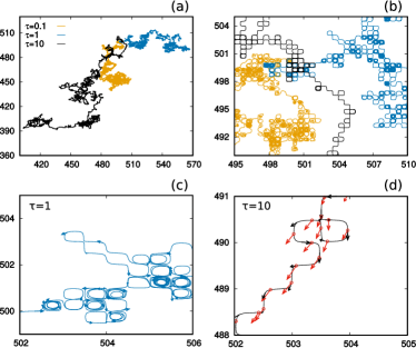
Figure 1: (a)-(b) panels: Snapshot of the trajectories for different values of $\tau=0.1,1,10$. (c)-(d) panels: enlargement for $\tau=1$ (c) and for $\tau=10$ (d). In panel (c) the arrows represent the velocity of the particle. In panel (c), the black arrows denote the velocity, while the red arrows denote the self-propulsion. The self-propulsion is rescaled for presentation reasons but here is $\sim 10^{-2}$ smaller than $U_{0}$. Simulations are realized with $D_{0}=10^{-2}$. The other parameters are $U_{0}=1$ and $L=1$.

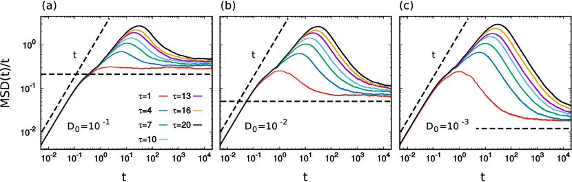
Figure 2: $\mathrm{MSD}(t)/t$ as a function of $t$ for different values of $\tau$, namely $\tau=1,4,7,10,13,16,20$ from the bottom to the top as shown in the legend. Panels (a), (b) and (c) are obtained with three different values of $D_{0}=10^{-1},10^{-2},10^{-3}$ from the left to the right. Dashed black lines mark linear and constant behaviors (corresponding on the ballistic and diffusive regimes of the $\mathrm{MSD}(t)$, respectively). The other parameters are $U_{0}=1$ and $L=1$.

We carry out a numerical study of the active dynamics (1) and (2) that are integrated via a second order stochastic Runge-Kutta algorithm Honeycutt (1992) with a time step $h=10^{-3}$ and for a time at least $2\times 10^{2}\,\tau$. Simulations are performed keeping fixed the cellular structure, $L=1$, $U_{0}=1$, in such a way that $T_{U}=1$, and evaluating the influence of the parameters $\tau$ and $D_{0}$ on the dynamics.

III.1 Single particle trajectories

We start by studying qualitatively the typical trajectories of the SPP in different relevant regimes. These observations will help us to understand the average properties showed by the mean square displacement and by the diffusion coefficient. In particular, in Fig. 1 (a), we compare different single-particle trajectories obtained for three different values of $\tau=10^{-1},1,10$ at fixed $D_{0}=10^{-2}$. For $\tau\ll T_{U}$ (yellow trajectory), the persistence feature of the self-propulsion is not relevant since $\mathbf{w}$ changes direction many times inside a single cell. As a consequence, the self-propulsion is indistinguishable from a thermal one and $\mathbf{w}$ behaves as a thermal noise with diffusivity $D_{0}$ (see Sec. III C).

For $\tau\gg T_{U}$ (black trajectory), the self-propulsion changes only after that the particle has crossed many cells. In these regimes, the average speed of self-propulsion is very small, decreasing as $1/\sqrt{\tau}$, since $D_{0}$ is fixed. As shown in panels (b) and (d) of Fig. 1, the particle proceeds along the separatrix between different vortices, and explores the regions where the cellular flow assumes its maximal value. The particle does not explore the region inside the cell and quite rarely becomes trapped in a vortex. This event is rarer as $\tau$ is increased. As a consequence, the self-propelled particle moves in a zig-zag-like way with a trajectory displaying an almost deterministic behavior that follows the flow field as shown in Fig. 1 (d). Due to the small value of the self-propulsion compared to $U_{0}$, $\mathbf{w}$ plays a role only in a small region near the nodes of the separatrix (where the flow field is zero). In those regions, the direction of $\mathbf{w}$ determines which one of the two separatrices the particle will follow. Moreover, since the average change of the self-propulsion direction is ruled by $\tau$, the same separatrix will be preferred for times smaller than $\tau$. This results in a unidirectional motion (along the separatrices) for small times ($<\tau$), in analogy with a free active particle with velocity $U_{0}$, while a diffusive-like behavior will be obtained for times larger than $T_{U}$.

For intermediate values of $\tau$, i.e. when $\tau\sim T_{U}$, the trajectory is more complicated, as illustrated in Fig.1 (c). The self-propulsion can deviate the trajectory from the cellular flow and push the SPP inside a vortex. The exit from the vortex can be determined by a fluctuation of the self-propulsion. A particle needs more time with respect to the thermal case to escape and proceed along the separatrix.

III.2 Mean Square Displacement

The rescaled mean square displacement (MSD) of the SPP, $\langle[x(t)-x(0)]^{2}\rangle/t$, averaged over thousands of realizations, is reported for several values of $\tau$ and three values of $D_{0}$ (Fig. 2 (a)-(c)). The $\mathrm{MSD}(t)$ reflects the behaviors of the single-particle trajectories: we identify short-time ballistic, intermediate-time anomalous diffusive and long-time diffusive regimes. In the small-$\tau$ limit, such that $\tau<\tau^{*}$, ballistic regimes occur for $t<\tau$ (not shown in the figure), in analogy with active particles in a homogeneous environment Caprini and Marconi (2019). When $\tau>\tau^{*}$, deviations from ballistic regimes occur for $t>\tau^{*}$, as reported in Fig. 2 (a)-(c). As shown in each panel, this regime weakly depends on $\tau$ and $D_{0}$ since for small $t$ the MSD collapses onto the same curve, at variance with active particles in homogeneous environments. A second regime occurs in the range of times $\tau^{*}<t<\tau$ where diffusion is slower but still superdiffusive, until a maximum of $\langle[x(t)-x(0)]^{2}\rangle/t$ is observed for $t\sim\tau$. After this maximum, the diffusivity slows down (the crossover appears as a transient sub-diffusion) and gets to normal diffusion asymptotically. The comparison between the different panels of Fig. 2 suggests that the anomalous diffusive regimes are less pronounced as $D_{0}$ increases even if, in all the cases, the anomalous diffusion region enlarges as $\tau$ grows. At large times, after $t>\tau_{D}$, the diffusive behavior is reached. Remarkably, the transient regime has a quite long duration, and the typical time $\tau_{D}$ increases with $\tau$ and decreases with $D_{0}$. We remark that the slowing down of the dynamics at intermediate times is related to the trapping effect due to the vortices of the cellular flow, which confines the particle motion in a limited region for a certain time.

III.3 Diffusion coefficient

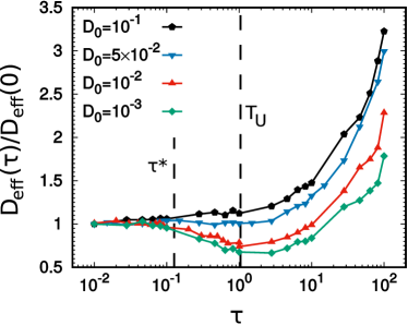
Figure 3: Effective diffusion coefficient as a function of $\tau$, for several values of $D_{0}$ as shown in the legend. The two dashed black lines are eye-guides which mark the value of $\tau^{*}$ and $T_{U}$. The other parameters are $U_{0}=1$ and $L=1$.

To unveil the effect of the self-propulsion force on the long-time diffusive dynamics, we study the diffusion coefficient

$$D_{\mathrm{eff}}=\lim_{t\to\infty}\frac{1}{2t}\langle[x(t)-x(0)]^{2}\rangle\,,$$ (5)

as a function of the activity parameters, $\tau$ and $D_{0}$. The case $\tau=0$ corresponds to the passive Brownian limit, where the leading contribution to the diffusion comes from the particles which move on the separatrices, and for which an analytical prediction has been computed by Shraiman in Shraiman (1987):

$$D_{\mathrm{eff}}(\tau=0)=\frac{S(k=1)}{\sqrt{\pi}}\sqrt{\dfrac{U_{0}LD_{0}}{2\pi}}\,.$$ (6)

Here, the function $S(k)$ depends on the cell geometry and is reported in Ref. Shraiman (1987). For the setup employed in the numerical study of this manuscript, we have $S(k=1)/\sqrt{\pi}\simeq 1.07$. We remark that the cellular flow enhances the diffusivity at small $D_{0}$, with respect to the case of homogeneous environments, producing a scaling $\sim\sqrt{D_{0}}$ instead of $\sim D_{0}$.

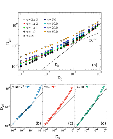
Figure 4: Effective diffusion coefficient, $D_{\mathrm{eff}}$, vs. $D_{0}$ for different values of $\tau$, as shown in the legend (panel (a)). The dashed black lines are eye guides showing the behavior $\sim D_{0}$ and $\sim\sqrt{D_{0}}$. Panels (b), (c) and (d) compare a curve of $D_{\mathrm{eff}}$ (for a given $\tau$) with the behavior $\propto\sqrt{D_{0}}$. The other parameters are $U_{0}=1$ and $L=1$.

In Fig. 3, we plot $D_{\mathrm{eff}}(\tau)/D_{\mathrm{eff}}(0)$ as a function of $\tau$ for four values of $D_{0}$ to show the role of the self-propulsion persistence. As expected, at small values of $\tau$, the prediction (6) is in agreement with numerical simulations since the self-propulsion acts as an effective thermal noise, in this regime. Depending on the value of $D_{0}$, we observe a different phenomenology. In particular, for the larger values of $D_{0}$, for instance $D_{0}=10^{-1}$ (or larger), $D_{\mathrm{eff}}$ grows with $\tau$ and, thus, the effect of increasing the persistence time is to enhance the diffusivity, even if the effective velocity decreases as $\sqrt{D_{0}/\tau}$. More surprisingly, for the smaller values of $D_{0}$, we obtain a non-monotonic behavior: In a regime of $\tau$ comparable with $T_{U}$, starting from $\tau^{*}=1/kU_{0}$, we observe that $D_{\mathrm{eff}}$ decreases down to a minimum value which is reached at times close to $T_{U}$. We remark that $\tau^{*}$ is the value of $\tau$ for which the overdamped approach for small $\tau$ does not hold, as shown in detail in Appendix A. After the minimum is reached, $D_{\mathrm{eff}}$ grows indefinitely. In particular, for $\tau$ large enough we observe $D_{\mathrm{eff}}>D_{\mathrm{eff}}(\tau=0)$ as in cases with larger $D_{0}$.

These observations are in agreement with the phenomenology characterizing the single-particle trajectories (Fig. 1). Indeed, the possibility of being trapped into a vortex for long times - seen for values of $\tau\sim T_{U}$ - is coherent with the observed reduction of $D_{\mathrm{eff}}$ in a range of $\tau$. Also, the observation of trajectories running fast along the separatrices for large values of $\tau$ is compatible with the final growth of $D_{\mathrm{eff}}$ (asymptotically for large $\tau$). Using this information, in the next section, we will derive an analytical prediction for $D_{\mathrm{eff}}$, in the regime $\tau\gg T_{U}$.

In panel (a) of Fig. 4, we show $D_{\mathrm{eff}}$ as a function of $D_{0}$ for several values of $\tau$ to test Shraiman’s scaling with $D_{0}$. As shown in panel (b) of Fig. 4, for $\tau\ll T_{U}$, $D_{\mathrm{eff}}\sim\sqrt{D_{0}}$, in agreement with Eq. (6). Shraiman’s scaling breaks down for large values of $D_{0}$, where $D_{\mathrm{eff}}\propto D_{0}$, occurring when $\mathbf{w}$ becomes comparable with $U_{0}$ and the cellular-flow plays a marginal role in the transport process. In Fig. 4 (c), we observe that Shraiman’s scaling does not hold for the intermediate values of $\tau$ (the region of $\tau$ corresponding to the minimum in Fig. 3), while it is recovered in the regime of large $\tau$, namely for $\tau\gg T_{U}$, even if the values of $D_{\mathrm{eff}}$ are quite larger with respect to Eq. (6), see panel (d).

IV Analytical prediction of $D_{\mathrm{eff}}$ for large persistence

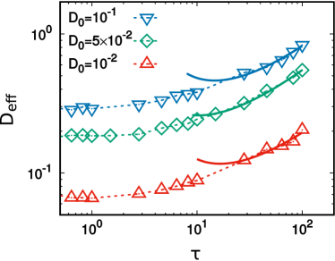
Figure 5: Effective diffusion coefficient vs. $\tau$ for two different values of $D_{0}$ (colored data). The solid lines are obtained from numerical fits of the prediction (10), namely $g(\tau)=a*\tau/\log^{2}(2U_{0}^{2}\tau/D_{0}/b)$, where $a$ and $b$ are two parameters. In particular, $b\approx 6$ does not depend on $D_{0}$ and $T_{U}$ and is just a numerical factor. The parameters of the numerical study are $U_{0}=1$ and $L=1$.

In the large persistence regime, $\tau\gg T_{U}$, the study of the single-particle trajectory has revealed that the SPP runs almost deterministically along the separatrices choosing the “same” direction for a time of order $\tau$. The change of direction occurs after a time $\sim\tau$, as it happens for an active particle in a homogeneous environment. In this simple case, the MSD, at large times, is given by

$$\mathrm{MSD}(t\gg\tau)\approx{\mathcal{L}}^{2}n=\left(\sqrt{D_{0}\tau}\right)^{2}\frac{t}{\tau}\,,$$ (7)

where ${\mathcal{L}}=\sqrt{D_{0}\tau}$ is the persistence length and $n=t/\tau$ counts the number of persistence lengths covered by the free-particle in the time $t$.

We consider the MSD of a self-propelled particle in the absence of cellular flow and replace the persistence length in a homogeneous environment ${\mathcal{L}}$ with the persistence length ${\mathcal{L}}_{\mathrm{eff}}$ of a particle moving in the laminar flow along the separatrices, with velocity $U_{0}\sin{\left(kx\right)}$ for $x\in[0,L/2]$ (obtained from Eq. (1)). Thus, at large times, we get the estimate

$$\mathrm{MSD}(t\gg\tau)\approx{\mathcal{L}}_{\mathrm{eff}}^{2}\frac{t}{\tau}=\left(\frac{L}{2\sqrt{2}}\frac{\tau}{t_{U}}\right)^{2}\frac{t}{\tau}\,,$$ (8)

where $t_{U}$ is the typical time to run for $L/2$ along a separatrix and is calculated in Appendix B. We remark that the validity of Eq. (8) is restricted to $\tau\gg T_{U}$, a regime where $\mathbf{w}$ plays a role only on the nodes of the separatrices because $|\mathbf{w}|<U_{0}$.

This argument suggests that the diffusion coefficient increases linearly with $\tau$ and does not depend on $D_{0}$, except for a dependence contained in $t_{U}$. In particular, we get (see Appendix B)

$$t_{U}\approx\frac{L}{U_{0}2\pi}\log{\left[\frac{2}{b}\frac{\tau}{D_{0}}{U_{0}^{2}}\right]}\,,$$ (9)

in the limit $\sqrt{D_{0}}/\sqrt{\tau}\ll U_{0}$. The parameter $b$ is just a numerical factor which does not depend on $\tau$, $D_{0}$ and $T_{U}$. In this regime, the prediction for the diffusion coefficient, for $\tau\gg t_{U}$ (calculated for $t\gg\tau$), reads:

$$D_{\mathrm{eff}}\propto\dfrac{U_{0}^{2}\,\tau}{\log^{2}{\left[\frac{2}{b}{U_{0}^{2}}\frac{\tau}{D_{0}}\right]}}\,.$$ (10)

The comparison between prediction and numerical data is reported in Fig. 5 as a function of $\tau$ for three different values of $D_{0}$. The results are in good agreement for $\tau\gg T_{U}$, while marked deviations emerge for $\tau\sim T_{U}$, where the main hypothesis behind Eq. (10) does not apply.

V Conclusion

In this manuscript, we have studied the diffusive properties of a self-propelled particle moving in a steady laminar flow, evaluating the effect of the self-propulsion. The diffusion coefficient displays a non-monotonic behavior as a function of the persistence time $\tau$: in particular, a minimum occurs for a large range of $D_{0}$ when $\tau$ is comparable with the turnover time, followed by a sharp increase, faster than $\tau$, such that the value of the diffusion coefficient exceeds Shraiman’s prediction valid in the passive Brownian case. Such a mechanism is discussed and connected to the single-particle trajectory, specifically to the occurrence of a trapping mechanism into the vortices. Additionally, Shraiman’s scaling with the diffusion coefficient is tested in the active case, revealing an intriguing scenario.

Our study shows that the presence of the self-propulsion affects the diffusion in a complex environment and could represent a mechanism naturally developed by self-propelled agents to improve the efficiency of the transport. Testing the presence of similar nonmonotonic behaviors in other inhomogeneous environments, going beyond the specific functional form of a laminar flow field, could be a promising research line to understand the behavior of self-propelled microorganisms in their complex habitats.

Appendix A Failure of the UCNA approximation

By taking the time derivative of the equation of motion (1), we get:

$$\ddot{\mathbf{r}} =\nabla\mathbf{A}(\mathbf{r})\;\dot{\mathbf{r}}+\dot{\mathbf{w}}$$ (11)

$$\tau\dot{\mathbf{w}} =-\mathbf{w}+\sqrt{2D_{0}}\;\boldsymbol{\xi}\,,$$ (12)

where the matrix $\nabla\mathbf{A}$ reads:

$$\nabla\mathbf{A} =kU_{0}\begin{bmatrix}\cos{\left(kx\right)}\cos{\left(ky\right)}\quad&-\sin{\left(kx\right)}\sin{\left(ky\right)}\\ \\ \sin{\left(kx\right)}\sin{\left(ky\right)}\quad&-\cos{\left(kx\right)}\cos{\left(ky\right)}\end{bmatrix}$$

$$=k^{2}\left[\begin{array}[]{cc}\phi{}&-\psi\\ \psi{}&-\phi\end{array}\right]\,,$$

being $\psi$ the stream function defined by Eq. (3) and

$$\phi(\mathbf{r})=\frac{U_{0}}{k}\cos{(kx)}\cos{(ky)}\,.$$

Adopting the usual change of variable $\mathbf{v}=\dot{\mathbf{r}}$, $\mathbf{v}=\mathbf{A}(\mathbf{r})+\mathbf{w}$, we obtain

$$\tau\dot{\mathbf{v}}=\boldsymbol{\Gamma}\mathbf{v}+\mathbf{A}(\mathbf{r})+\sqrt{2D_{0}}\boldsymbol{\xi}\,,$$ (13)

where the matrix $\boldsymbol{\Gamma}$ assumes the simple form:

$$\boldsymbol{\Gamma}(\mathbf{r})=\mathcal{I}-\tau\nabla\mathbf{A}(\mathbf{r})\,,$$ (14)

and $\mathcal{I}$ is the identity matrix. For those values of $\tau$ such that the matrix $\boldsymbol{\Gamma}$ is no longer positive-defined, the overdamped limit needed for UCNA becomes meaningless. We recall that a diagonalizable matrix is positive-defined when all its eigenvalues are positive. The eigenvalues of the matrix $\boldsymbol{\Gamma}$ (Eq. (14)) read:

$$\lambda_{1} =1-\tau k^{2}\sqrt{\phi^{2}-\psi^{2}}$$

$$\lambda_{2} =1+\tau k^{2}\sqrt{\phi^{2}-\psi^{2}}\,.$$

Using the definition of $\psi(x,y)$ and $\phi(x,y)$, after some algebraic manipulations, we obtain

$$\lambda_{1} =1-\tau kU_{0}\sqrt{\cos[k(x-y)]\cos[k(x+y)]}$$

$$\lambda_{2} =1+\tau kU_{0}\sqrt{\cos[k(x-y)]\cos[k(x+y)]}$$

When $\tau\geq\tau^{*}=1/(U_{0}k)$, the eigenvalue $\lambda_{1}$ has no possibility to be positive globally in space, then $\boldsymbol{\Gamma}$ cannot be positive definte and the overdamped regime turns to be undefined. In the opposite regime, $\tau<\tau^{*}$, which we call small-$\tau$ limit, the overdamped regime could be assumed. Only, in the latter case, the dynamics can be recast onto:

$$\boldsymbol{\Gamma}\,{\mathbf{v}}={\mathbf{A}}({\mathbf{r}})+\sqrt{2D_{0}}\;{\mathbf{\xi}}\,.$$ (15)

By inversion we obtain:

$$\dot{\mathbf{r}}={\mathbf{v}}=\boldsymbol{\Gamma}^{-1}\bigg{(}{\mathbf{A}}({\mathbf{r})}+\sqrt{2D_{0}}\;{\mathbf{\xi}}\bigg{)}\,,$$ (16)

which corresponds to the UCNA dynamics Maggi et al. (2015) adapted to the current case.

We remark that $\tau^{*}$ roughly corresponds to the value of $\tau$ at which $D_{\mathrm{eff}}$ starts to consistently change with respect to the Shraiman’s prediction, as shown in Fig. 3.

Appendix B Computation of $t_{U}$ in the regime of large $\tau$

The typical time $t_{U}$ contained in Eqs. (8) and (9) can be obtained by integrating Eq. (1) without the self-propulsion in a given direction along a separatrix, for instance:

$$t_{U}=\frac{1}{U_{0}}\int_{0}^{L/2}\frac{dx}{\sin{(2\pi x/L)}}\,.$$ (17)

This procedure is justified because the active force is negligible along the separatrices, except for the nodes, in the large persistence regime. The integral defining $t_{U}$ is not converging, unless we introduce two cut-offs

$$t_{U} =\frac{1}{U_{0}}\int_{x_{m}}^{L/2-x_{m}}\frac{dx}{\sin{(2\pi x/L)}}\,.$$ (18)

The length scale $x_{m}$ is chosen such as:

$$U_{0}\sin{\left(kx_{m}\right)}=\sqrt{2\,b\,\frac{D_{0}}{\tau}}\,,$$ (19)

i.e. when the force along a separatrix is roughly equal to the typical value of the activity, estimated by its standard deviation, $\sqrt{D_{0}/\tau}$. The factor $b$ is a parameter that does not depend on $\tau$, $D_{0}$ and $T_{U}$, being just a numerical factor. Inverting Eq. (19), we get

$$x_{m}=\frac{L}{2\pi}\arcsin{\left(\sqrt{\frac{2\,b\,D_{0}}{\tau}}\frac{1}{U_{0}}\right)}\approx\frac{L}{U_{0}\pi}\sqrt{\frac{b\,D_{0}}{2\tau}}\,,$$

where we have used the condition $\sqrt{D_{0}/\tau}\ll U_{0}=1$ holding in the large persistence regime. Solving the integral, we obtain the final expression for $t_{U}$,

$$t_{U}\frac{U_{0}\pi}{L}= \log{\left(\frac{1}{\tan{\left[\sqrt{\frac{b\,D_{0}}{2\tau}}\frac{1}{U_{0}}\right]}}\right)}\approx\frac{1}{2}\log{\left(\frac{2U^{2}_{0}}{b}\frac{\tau}{D_{0}}\right)}\,,$$

which is positive since $U_{0}\sqrt{\tau/D_{0}}\gg 1$. Thus, from Eq. (B), $t_{U}$ contains a dependence on $D_{0}/\tau$ which scales as $\log{(\tau/D_{0})}$, as reported in Eq. (9).

References

- Bechinger et al. (2016) C. Bechinger, R. Di Leonardo, H. Löwen, C. Reichhardt, G. Volpe, and G. Volpe, Reviews of Modern Physics 88, 045006 (2016).
- Marchetti et al. (2013) M. C. Marchetti, J. F. Joanny, S. Ramaswamy, T. B. Liverpool, J. Prost, M. Rao, and R. A. Simha, Rev. Mod. Phys. 85, 1143 (2013).
- Buttinoni et al. (2013) I. Buttinoni, J. Bialké, F. Kümmel, H. Löwen, C. Bechinger, and T. Speck, Phys. Rev. Lett. 110, 238301 (2013).
- Palacci et al. (2013) J. Palacci, S. Sacanna, A. Steinberg, D. Pine, and P. Chaikin, Science , 1230020 (2013).
- Ginot et al. (2018) F. Ginot, I. Theurkauff, F. Detcheverry, C. Ybert, and C. Cottin-Bizonne, Nat. Comm. 9, 696 (2018).
- Fily and Marchetti (2012) Y. Fily and M. C. Marchetti, Phys. Rev. Lett. 108, 235702 (2012).
- Bialké et al. (2015) J. Bialké, T. Speck, and H. Löwen, J. Non-Cryst. Solids 407, 367 (2015).
- Cates and Tailleur (2015) M. E. Cates and J. Tailleur, Annu. Rev. Condens. Matter Phys. 6, 219 (2015).
- Digregorio et al. (2018) P. Digregorio, D. Levis, A. Suma, L. F. Cugliandolo, G. Gonnella, and I. Pagonabarraga, Physical review letters 121, 098003 (2018).
- Solon et al. (2018) A. P. Solon, J. Stenhammar, M. E. Cates, Y. Kafri, and J. Tailleur, New Journal of Physics 20, 075001 (2018).
- Chiarantoni et al. (2020) P. Chiarantoni, F. Cagnetta, F. Corberi, G. Gonnella, and A. Suma, arXiv preprint arXiv:2001.08500 (2020).
- Caprini et al. (2020) L. Caprini, U. M. B. Marconi, and A. Puglisi, Physical Review Letters 124, 078001 (2020).
- Lam et al. (2015) K.-D. N. T. Lam, M. Schindler, and O. Dauchot, New Journal of Physics 17, 113056 (2015).
- Ginelli et al. (2010) F. Ginelli, F. Peruani, M. Bär, and H. Chaté, Phys. Rev. Lett. 104, 184502 (2010).
- Sumino et al. (2012) Y. Sumino, K. H. Nagai, Y. Shitaka, D. Tanaka, K. Yoshikawa, H. Chaté, and K. Oiwa, Nature 483, 448 (2012).
- ten Hagen et al. (2011) B. ten Hagen, S. van Teeffelen, and H. Löwen, Journal of Physics: Condensed Matter 23, 194119 (2011).
- Sevilla and Nava (2014) F. J. Sevilla and L. A. G. Nava, Physical Review E 90, 022130 (2014).
- Basu et al. (2018) U. Basu, S. N. Majumdar, A. Rosso, and G. Schehr, Physical Review E 98, 062121 (2018).
- Scholz et al. (2018) C. Scholz, S. Jahanshahi, A. Ldov, and H. Löwen, Nature communications 9, 1 (2018).
- Sevilla and Castro-Villarreal (2019) F. J. Sevilla and P. Castro-Villarreal, arXiv preprint arXiv:1912.03425 (2019).
- Caprini and Marconi (2019) L. Caprini and U. M. B. Marconi, Soft matter 15, 2627 (2019).
- Miño et al. (2018) G. Miño, M. Baabour, R. Chertcoff, G. Gutkind, E. Clément, H. Auradou, and I. Ippolito, Adv. Microbiol. 8, 451 (2018).
- Li and Tang (2009) G. Li and J. X. Tang, Phys. Rev. Lett. 103, 078101 (2009).
- Wensink and Löwen (2008) H. Wensink and H. Löwen, Phys. Rev. E 78, 031409 (2008).
- Elgeti and Gompper (2013) J. Elgeti and G. Gompper, EuroPhysics Lett. 101, 48003 (2013).
- Wittmann and Brader (2016) R. Wittmann and J. M. Brader, EPL (Europhysics Letters) 114, 68004 (2016).
- Das et al. (2020) S. Das, S. Ghosh, and R. Chelakkot, arXiv preprint arXiv:2001.04654 (2020).
- Caprini et al. (2019a) L. Caprini, F. Cecconi, and U. Marconi Marini Bettolo, J. Chem. Phys. 150 (2019a).
- Ford and Harvey (2007) R. M. Ford and R. W. Harvey, Advances in Water Resources 30, 1608 (2007).
- Engstler et al. (2007) M. Engstler, T. Pfohl, S. Herminghaus, M. Boshart, G. Wiegertjes, N. Heddergott, and P. Overath, Cell 131, 505 (2007).
- Ribet and Cossart (2015) D. Ribet and P. Cossart, Microbes and Infection 17, 173 (2015).
- Chepizhko and Peruani (2013) O. Chepizhko and F. Peruani, Physical review letters 111, 160604 (2013).
- Chepizhko et al. (2013) O. Chepizhko, E. G. Altmann, and F. Peruani, Physical review letters 110, 238101 (2013).
- Majmudar et al. (2012) T. Majmudar, E. E. Keaveny, J. Zhang, and M. J. Shelley, Journal of the Royal Society Interface 9, 1809 (2012).
- Brown et al. (2016) A. T. Brown, I. D. Vladescu, A. Dawson, T. Vissers, J. Schwarz-Linek, J. S. Lintuvuori, and W. C. Poon, Soft Matter 12, 131 (2016).
- Volpe et al. (2011) G. Volpe, I. Buttinoni, D. Vogt, H.-J. Kümmerer, and C. Bechinger, Soft Matter 7, 8810 (2011).
- Khatami et al. (2016) M. Khatami, K. Wolff, O. Pohl, M. R. Ejtehadi, and H. Stark, Scientific reports 6, 37670 (2016).
- Sándor et al. (2017) C. Sándor, A. Libál, C. Reichhardt, and C. Olson Reichhardt, The Journal of chemical physics 146, 204903 (2017).
- Kaiser et al. (2012) A. Kaiser, H. Wensink, and H. Löwen, Physical review letters 108, 268307 (2012).
- Tailleur and Cates (2009) J. Tailleur and M. Cates, EPL (Europhysics Letters) 86, 60002 (2009).
- Wan et al. (2008) M. Wan, C. O. Reichhardt, Z. Nussinov, and C. Reichhardt, Physical review letters 101, 018102 (2008).
- Volpe et al. (2014) G. Volpe, S. Gigan, and G. Volpe, American Journal of Physics 82, 659 (2014).
- Galajda et al. (2007) P. Galajda, J. Keymer, P. Chaikin, and R. Austin, Journal of bacteriology 189, 8704 (2007).
- Bénichou et al. (2015) O. Bénichou, P. Illien, G. Oshanin, A. Sarracino, and R. Voituriez, Phys. Rev. Lett. 115, 220601 (2015).
- Jakuszeit et al. (2019) T. Jakuszeit, O. A. Croze, and S. Bell, Physical Review E 99, 012610 (2019).
- Pattanayak et al. (2019) S. Pattanayak, R. Das, M. Kumar, and S. Mishra, The European Physical Journal E 42, 62 (2019).
- Reichhardt and Reichhardt (2018) C. Reichhardt and C. O. Reichhardt, Physical Review E 97, 052613 (2018).
- Morin et al. (2017) A. Morin, N. Desreumaux, J.-B. Caussin, and D. Bartolo, Nature Physics 13, 63 (2017).
- Zeitz et al. (2017) M. Zeitz, K. Wolff, and H. Stark, The European Physical Journal E 40, 23 (2017).
- Aragones et al. (2018) J. L. Aragones, S. Yazdi, and A. Alexander-Katz, Physical Review Fluids 3, 083301 (2018).
- Barkai et al. (2012) E. Barkai, Y. Garini, and R. Metzler, Phys. Today 65, 29 (2012).
- Shaebani et al. (2014) M. R. Shaebani, Z. Sadjadi, I. M. Sokolov, H. Rieger, and L. Santen, Physical Review E 90, 030701 (2014).
- Woillez et al. (2019a) E. Woillez, Y. Kafri, and N. Gov, arXiv preprint arXiv:1910.02667 (2019a).
- Shraiman (1987) B. I. Shraiman, Physical Review A 36, 261 (1987).
- Taylor (1953) G. I. Taylor, Proceedings of the Royal Society of London. Series A. Mathematical and Physical Sciences 219, 186 (1953).
- Thorpe (2004) S. Thorpe, Annu. Rev. Fluid Mech. 36, 55 (2004).
- Alonso-Matilla et al. (2019) R. Alonso-Matilla, B. Chakrabarti, and D. Saintillan, Physical Review Fluids 4, 043101 (2019).
- Durham et al. (2013) W. M. Durham, E. Climent, M. Barry, F. D. Lillo, G. Boffetta, M. Cencini, and R. Stocker, Nat. Comm. 4, 2148 (2013).
- Santamaria et al. (2014) F. Santamaria, F. D. Lillo, M. Cencini, and G. Boffetta, Phys. Fluids 26, 111901 (2014).
- Rusconi et al. (2014) R. Rusconi, J. S. Guasto, and R. Stocker, Nat. Phys. 10, 212 (2014).
- Junot et al. (2019) G. Junot, N. Figueroa-Morales, T. Darnige, A. Lindner, R. Soto, H. Auradou, and E. Clément, EPL (Europhysics Letters) 126, 44003 (2019).
- Castiglione and Crisanti (1999) P. Castiglione and A. Crisanti, Physical Review E 59, 3926 (1999).
- Torney and Neufeld (2007) C. Torney and Z. Neufeld, Physical review letters 99, 078101 (2007).
- Sarracino et al. (2016) A. Sarracino, F. Cecconi, A. Puglisi, and A. Vulpiani, Physical review letters 117, 174501 (2016).
- Cecconi et al. (2017) F. Cecconi, A. Puglisi, A. Sarracino, and A. Vulpiani, The European Physical Journal E 40, 81 (2017).
- Cecconi et al. (2018) F. Cecconi, A. Puglisi, A. Sarracino, and A. Vulpiani, Journal of Physics: Condensed Matter 30, 264002 (2018).
- Li et al. (2020) Y. Li, L. Li, F. Marchesoni, D. Debnath, and P. K. Ghosh, arXiv preprint arXiv:2002.06113 (2020).
- Das et al. (2018) S. Das, G. Gompper, and R. Winkler, New J. Phys. 20, 015001 (2018).
- Fodor et al. (2016) E. Fodor, C. Nardini, M. E. Cates, J. Tailleur, P. Visco, and F. van Wijland, Phys. Rev. Lett. 117, 038103 (2016).
- Caprini et al. (2019b) L. Caprini, U. M. B. Marconi, A. Puglisi, and A. Vulpiani, Journal of Statistical Mechanics: Theory and Experiment 2019, 053203 (2019b).
- Wittmann et al. (2019) R. Wittmann, F. Smallenburg, and J. M. Brader, The Journal of chemical physics 150, 174908 (2019).
- Berthier et al. (2019) L. Berthier, E. Flenner, and G. Szamel, The Journal of chemical physics 150, 200901 (2019).
- Woillez et al. (2019b) E. Woillez, Y. Kafri, and V. Lecomte, arXiv preprint arXiv:1912.04010 (2019b).
- Marconi et al. (2016) U. M. B. Marconi, N. Gnan, M. Paoluzzi, C. Maggi, and R. Di Leonardo, Sci. Rep. 6, 23297 (2016).
- Maggi et al. (2014) C. Maggi, M. Paoluzzi, N. Pellicciotta, A. Lepore, L. Angelani, and R. Di Leonardo, Physical review letters 113, 238303 (2014).
- Maggi et al. (2017) C. Maggi, M. Paoluzzi, L. Angelani, and R. Di Leonardo, Scientific reports 7, 1 (2017).
- Maggi et al. (2015) C. Maggi, U. M. B. Marconi, N. Gnan, and R. Di Leonardo, Scientific reports 5, 10742 (2015).
- Caprini et al. (2019c) L. Caprini, U. M. B. Marconi, and A. Puglisi, Sci. Rep. 9, 1386 (2019c).
- Caprini et al. (2019d) L. Caprini, U. Marini Bettolo Marconi, A. Puglisi, and A. Vulpiani, The Journal of Chemical Physics 150, 024902 (2019d).
- Honeycutt (1992) R. L. Honeycutt, Physical Review A 45, 600 (1992).