Abstract

Bayesian statistical inference loses predictive optimality when generative models are misspecified.

Working within an existing coherent loss-based generalisation of Bayesian inference, we show existing Modular/Cut-model inference is coherent, and write down a new family of Semi-Modular Inference (SMI) schemes, indexed by an influence parameter, with Bayesian inference and Cut-models as special cases. We give a meta-learning criterion and estimation procedure to choose the inference scheme. This returns Bayesian inference when there is no misspecification.

The framework applies naturally to Multi-modular models. Cut-model inference allows directed information flow from well-specified modules to misspecified modules, but not vice versa. An existing alternative power posterior method gives tunable but undirected control of information flow, improving prediction in some settings. In contrast, SMI allows tunable and directed information flow between modules.

We illustrate our methods on two standard test cases from the literature and a motivating archaeological data set.

1 Introduction

Consider statistical inference in a multi-modular setting. The model for the available data is assembled from several component modules. Each module describes a probabilistic relation between observable variables (data) and unknown quantities (parameters, latent variables, missing data). Modules may share parameters, missing data and other latent variables. Fig. 1 illustrates a simple two-module model with a shared parameter $\varphi$ (ignore the dashed line explained in Sec. 2.1). The first module has data $Z$ and one parameter, $\varphi$, while the second module has data $Y$ and two parameters, $\theta$ and $\varphi$.

Figure 1: Graphical representation of a simple multi-modular model.

In conventional Bayesian inference, parameters are jointly informed by the data and model assumptions shared across the modules. As a consequence, large-scale multi-modular analyses are particularly susceptible to problems arising from model misspecification, as any bad module may distort inference in the model as a whole (Liu et al.,, 2009).

This drawback has motivated alternative inferential approaches that modify conventional Bayesian learning in order to regulate feedback between modules. Modular inference (Liu et al.,, 2009; Jacob et al., 2017a, ) also known as a Cut-model inference (Spiegelhalter et al.,, 2014; Plummer,, 2015) completely eliminates the contribution from some modules to the posterior distribution of parameters in other modules (see Section 2.1). However, we may do better to moderate, rather than eliminate, the influence of misspecified modules.

We give a new Semi-Modular Inference (SMI) which smoothly regulates the influence of modules on the overall inference. The procedure effectively expands the space of candidate distributions in such a way that Bayesian inference and Cut-model inference are particular cases.

When it comes to expanding the inference framework, an “anything goes” approach is clearly suspect. We stay within the class of inference schemes defined by Bissiri et al., (2016). Those authors define and characterise coherent loss-based inference and note that Bayesian inference and the power posterior (Walker and Hjort,, 2001) are coherent. We set out existing Cut-model and Power-posterior inference in Sections 2.1 and 2.2, introduce SMI in Section 3 and then describe the encompassing framework of Bissiri et al., (2016) in Section 4.1, where we show that SMI and Cut-model inference are coherent.

The SMI posterior interpolates candidate distributions between the conventional Bayesian posterior and the Cut-model posterior. Candidate distributions are indexed by a continuous degree of influence parameter $\eta$. This controls the contribution of a module to the candidate distribution. When $\eta$=0 the candidate distribution is the Cut-model posterior and when $\eta$=1 it is the Bayesian posterior. The SMI posterior is not a scheme for model elaboration with an extra parameter. SMI-based inference with any value of $\eta$ other than $\eta=1$ is not Bayesian inference.

In Section 5, we apply SMI to model-based inference for simulated and real-world datasets and evaluate its performance. It is easy to understand why it outperforms Bayesian and Modular inference in these examples. The supplementary material provides proofs and additional numerical experiments. All results are reproducible using the accompanying R package.

2 Background methods

2.1 Modular Inference: cut model

The Cut model is an alternative to Bayesian inference designed to remove unwanted feedback from poorly specified modules. The OpenBUGS manual (Spiegelhalter et al.,, 2014) describes the cut function with the words “The cut function acts as a kind of valve in the graph: prior information is allowed to flow downwards through the cut, but likelihood information is prevented from flowing upwards”. Cut model inference is a form of Bayesian multiple imputation.

Consider again the two-module configuration of Fig. 1. In standard joint or “full” Bayesian inference, information from the two modules informs every parameter, so in particular the values of $Y$ will in general influence the posterior distribution of $\varphi$. The posterior distribution of $(\varphi,\theta)$ in Bayesian inference is

$$p(\varphi,\theta\mid Z,Y)=p(\varphi\mid Z,Y)p(\theta\mid Y,\varphi).$$ (1)

The marginal distribution of $\varphi$ depends on $Y$.

Now, suppose that for some reason (usually because we suspect some model misspecification) we want the parameter $\varphi$ to learn only from module 1, cutting the influence from module 2 on $\varphi$. The cut is represented in Fig. 1 by a dashed line on the edge from $\varphi$ to $Y$; it denotes an inference structure in which $\varphi$ influences $Y$ but not vice versa (following Lunn et al., (2009)).

Under this modified scheme, the Cut-model “posterior” for $(\varphi,\theta)$ is

$$p_{cut}(\varphi,\theta\mid Z,Y)=p(\varphi\mid Z)p(\theta\mid Y,\varphi).$$ (2)

Notice that the marginal distribution of $\varphi$ no longer depends on $Y$.

Cut-model inference is a form of Bayesian Multiple Imputation (Lunn et al.,, 2009; Styring et al.,, 2017) in which we make multiple imputation of $\varphi$ and then analysis of $\theta$ given the imputated distribution of $\varphi$. The literature identifies potential advantages: cut models may simplify inference (Cox,, 1975); prevent unwanted feedback from suspect models (Lunn et al.,, 2009); improve MCMC mixing (Plummer,, 2015); reduce the MSE in estimates (Liu et al.,, 2009); increase predictive performance (Jacob et al., 2017a, ); answer the need in some settings to make a sequential analysis in which the data $Z$ is not shared with the analyst carrying out inference for $\theta$.

2.2 Power posterior

In the power posterior we raise the likelihood to a power, seeking to improve robustness under model misspecification (Walker and Hjort, (2001); Bissiri et al., (2016); Holmes and Walker, (2017); Grünwald and van Ommen, (2017); Miller and Dunson, (2018)).

Consider independent data $Y=(Y_{1},\ldots,Y_{n})$ generated from an unknown true distribution $f^{*}(Y)$. Assume we have a data model $f(Y|\theta)$ and a prior distribution $p(\theta)$. For a fixed $\eta\in\mathbb{R}$, we define the $\eta$-powered posterior $p_{pow,\eta}(\theta|x)$ as

$$p_{pow,\eta}(\theta|Y)=\frac{f(Y|\theta)^{\eta}p(\theta)}{p_{\eta}(Y)}\\$$ (3)

with $p_{\eta}(Y)=\int f(Y|\theta)^{\eta}p(\theta)d\theta$ the powered normalising constant.

The new parameter $\eta$ is called the learning rate, following Grünwald, (2012). The learning rate calibrates the influence of the prior relative to that of the data; if $\eta\in[0,1]$ the prior is given more influence and the data less. When $\eta>1$ the data is given more prominence, and in the extreme case when $\eta$ is very large the posterior accumulates around the maximum likelihood estimate for the model. For the misspecification we encounter, we tend to be interested in the case $\eta\in[0,1]$.

A key point emphasised by Grünwald and van Ommen, (2017) among others is that this is not simply model elaboration. We do not put a prior on $\eta$ and learn it in the usual Bayesian way. Roughly speaking the learning rate “corrects” Bayesian inference and should not be chosen using Bayesian inference but according to other “external” criteria, for example, a predictive loss on test data. Grünwald, (2012) and Grünwald and van Ommen, (2017) propose the SafeBayes algorithm to find the optimal learning rate. In that work, the learning rate $\eta$ is chosen to maximise the “sequentially randomised” Bayesian marginal log-likelihood. This can be interpreted as measure of predictive accuracy. In contrast Holmes and Walker, (2017) choose the learning rate by matching the prior expected gain in information between the prior and posterior. This gain in information is quantified by the expected divergence in Fisher information.

3 Semi-Modular Inference

In this section, we define Semi-Modular Inference (SMI), a modification of Bayesian inference in multi-modular settings which allows us to adjust the flow of information between data and parameters in separate modules. Referring to the two-module example in Fig. 1, we allow the data from module 1 to dominate in inference for $\varphi$ without entirely discarding the joint structure provided by the full model.

Our approach is motivated by the observation in Plummer, (2015) that cut-model inference is Bayesian multiple imputation: we might expect to do better at the second analysis stage of cut-model inference if we can more accurately impute missing values in the first stage. A two stage analysis resembling Cut-model analysis, but using a power posterior in the first stage delivers this. First, we update our beliefs about $\varphi$ using a power likelihood, with power $\eta\in[0,1]$ on module 2. The power-posterior improves Bayesian multiple imputation of $\varphi$ at the expense of $\theta$. In the second stage, we re-learn our beliefs on $\theta$ conditional on the learnt distribution of $\varphi$.The degree of influence, $\eta$, controls the contribution of the suspect module in the inference.

3.1 SMI distributions

Let $p(Z|\varphi)$ and $p(Y|\varphi,\theta)$ denote the observation models for the two modules. We introduce an auxiliary parameter $\tilde{\theta}$, expanding the model parameters from $(\varphi,\theta)$ to $(\varphi,\theta,\tilde{\theta})$.

We define the $\eta$-smi posterior as

$$p_{smi,\eta}(\varphi,\theta,\tilde{\theta}|Z,Y)=p_{pow,\eta}(\varphi,\tilde{\theta}|Z,Y)p(\theta|Y,\varphi)$$ (4)

where $p_{pow,\eta}(\varphi,\tilde{\theta}\mid Z,Y)$ is the power posterior

$$p_{pow,\eta}(\varphi,\tilde{\theta}\mid Z,Y)\propto p(Z|\varphi)p(Y\mid\varphi,\tilde{\theta})^{\eta}\;p(\varphi,\tilde{\theta}).$$ (5)

Expanding in terms of model elements (details in supplement),

$$p_{smi,\eta}(\varphi,\theta,\tilde{\theta}|Z,Y)\propto \;p(Z\mid\varphi)\;p(Y\mid\varphi,\tilde{\theta})^{\eta}\;p(Y\mid\varphi,\theta)$$

$$\times\quad\frac{1}{p(Y\mid\varphi)}\;p(\varphi,\theta,\tilde{\theta}),$$

where $p(Y\mid\varphi)=\frac{1}{p(\varphi)}\int p(Y\mid\varphi,\theta)\;p(\varphi,\theta)d\theta$.

The $\eta$-smi posterior of the original parameters is just the marginal,

$$p_{smi,\eta}(\varphi,\theta|Z,Y)=\int p_{smi,\eta}(\varphi,\theta,\tilde{\theta}|Z,Y)d\tilde{\theta}.$$ (6)

The posterior distribution $p_{smi,\eta}(\varphi,\theta|Z,Y)$ interpolates between the Bayesian posterior and the Cut model posterior. When $\eta=1$ the SMI posterior is the usual Bayesian posterior (Eq. 1),

$$p_{smi,1}(\varphi,\theta|Z,Y) =p(\varphi|Z,Y)p(\theta|Y,\varphi)$$

$$=p(\varphi,\theta|Z,Y),$$

whereas if $\eta=0$, the SMI posterior of $\varphi$ gives back the Cut model (Eq. 2),

$$p_{smi,0}(\varphi,\theta|Z,Y) =p(\varphi|Z)p(\theta|Y,\varphi)$$

$$=p_{cut}(\varphi,\theta|Z,Y).$$

Semi-modular inference is defined for a fixed degree of influence $\eta\in[0,1]$. Each value of $\eta$ yields a different candidate distribution, $p_{smi,\eta}$, which we call the SMI posterior, representing posterior belief on $(\varphi,\theta)$. Natural questions now are, how to choose in a principled manner the “best” degree of influence, and how and why does SMI help? The answer to the latter question is in a sense straightforward. If a generalised inference scheme achieves a better score, according to some agreed external criterion, we should use it, and not otherwise. This approach is taken in Jacob et al., 2017a . We answer the first question in the next section.

4 Analysis with (Semi-)Modular Inference

In this section we show that inference with the SMI posterior distribution at fixed $\eta$ is valid (in the sense of Bissiri et al., (2016)) and give an MCMC algorithm targeting $p_{smi,\eta}(\varphi,\theta|Z,Y)$. We give criteria and estimation procedures for choosing $\eta$, and comment on relations with cut-models and the power posterior.

4.1 Coherence of (Semi-)Modular Inference

We apply the general framework for updating belief distributions in Bissiri et al., (2016) to show that the SMI posterior - and hence also the cut posterior - are valid and coherent updates of beliefs. This framework is based on a loss function $l(\theta;y)$ connecting information in the data to the parameters of interest. The log-likelihood is one such loss, but Bissiri et al., (2016) give examples where other losses may be relevant, and Cut-models and SMI prove to be further examples.

Bissiri et al., (2016) characterise a valid belief update. They list a number of axiomatic requirements. We verify that our SMI-update satisfies these axioms in the supplement. The most demanding of these conditions, in our setting, is the coherence condition.

In Coherent inference we reach the same posterior distribution, whether we update belief using all data simultaneously or update belief taking the data sequentially in independent blocks. In our two-module setting, this applies in several ways: we can observe responses from different modules one after the other (e.g. first $Z$, and then $Y$); we can observe sequential data fragments within the same module (e.g. first $Z_{1}$, and then $Z_{2}$, with $Z=(Z_{1},Z_{2})$); any mixture of these.

The generalised update of belief in Bissiri et al., (2016) follows a decision theoretic approach. In single module notation, the generalised posterior distribution $p_{l_{\rho}}$ arising from a loss $l_{\rho}(\theta;y)$ in a family of loss functions indexed by $\rho$, is the probability measure minimising a cumulative loss function $L_{\rho}(\nu;p_{0},Y)$ over choices of probability measure $\nu$,

$$p_{l_{\rho}}(\theta\mid Y)=\operatorname*{arg\,min}_{\nu}L_{\rho}(\nu;p_{0},Y).$$

The cumulative loss function, $L_{\rho}(\nu;p,Y)$ balances the expected loss in the fit to data and the Kullback-Leibler divergence from the posterior to the prior distribution (generically $p_{0}$ say), and is defined by

$$L_{\rho}(\nu;p_{0},Y)=\int l_{\rho}(\theta,Y)\nu(d\theta)+d_{KL}(\nu,p_{0}).$$

Bissiri et al., (2016) show that the optimal, valid and coherent update of beliefs from prior to posterior is given by

$$p_{l_{\rho}}(\theta\mid Y)\propto\exp\{-l_{\rho}(\theta;Y)\}p_{0}(\theta)$$

The canonical case in the single-module setting is the logarithmic loss function $l(\theta;Y)=-\log f(Y\mid\theta)$, which yields the conventional Bayesian update of beliefs given by the posterior distribution. The power posterior is obtained by taking the loss function $l_{pow,\rho}(\theta;Y)=-\rho\log f(Y\mid\theta)$.

In the Supplementary material we prove that, for the model in Fig. 1, the loss function which yields the Cut model posterior is

$$l_{cut}((\varphi,\theta);(Z,Y))= -\log p(Z\mid\varphi)$$ (7)

$$-\log p(Y\mid\varphi,\theta)+\log p(Y\mid\varphi),$$

and the loss function yielding the SMI posterior is

$$l_{smi,\eta}((\varphi,\theta,\tilde{\theta}); (Z,Y))=-\log p(Z\mid\varphi)$$ (8)

$$-\eta\log p(Y\mid\varphi,\tilde{\theta})$$

$$-\log p(Y\mid\varphi,\theta)+\log p(Y\mid\varphi).$$

The $p(Y\mid\varphi)$ terms in each expression are the loss-function expression of the idea of cutting feedback from $Y$ to $\varphi$.

We prove that both Cut-model inference and SMI are coherent when we update using the correct associated loss function given above. Detailed proofs are given in the supplementary material.

4.2 Targeting the modular posterior

Plummer, (2015) and Jacob et al., 2017a explain that an MCMC algorithm that correctly targets the cut distribution cannot usually be implemented, due to the presence of the intractable normalising constant $p(Y\mid\varphi)$. A SMI sampler faces the same issue.

In order to sample the SMI-posterior in a single MCMC run we need, refering to Eq. 4, a standard MCMC sampler for $p_{pow,\eta}(\varphi,\tilde{\theta}\mid Z,Y)$ and an exact sampler for $p(\theta\mid Y,\varphi)$. It is straightforward to check that the transition kernel given by a two-stage update using these two conditional distributions satisfies detailed balance. A proof is given in the supplement.

Exact simulation of $p(\theta\mid Y,\varphi)$ may be impracticable. In practice, there are currently three options, nested MCMC, unbiased MCMC via couplings (Jacob et al., 2017b, ), and tempered transitions (Plummer,, 2015).

Unbiased MCMC via couplings simulates samples unbiased in expectation from the Cut-model posterior. The approach uses coupled pairs of Markov Chains sharing a common transition kernel, which almost-surely meet at some finite time $\tau\geq 1$ and stay together thereafter. The same approach applies to SMI, though we have not implemented this.

In our examples we use nested MCMC, described in Algorithm 1: sample $N_{1}$ draws from $p_{pow,\eta}(\varphi,\tilde{\theta}\mid Z,Y)$; for each sampled value of $\varphi$, run a sub-chain targeting $p(\theta\mid\varphi,Z)$ for $N_{2}$ steps, where $N_{2}$ is large enough to avoid initialisation bias; keep only the last sampled value in this sub-chain. The resulting joint samples $(\varphi,\tilde{\theta},\theta)$ are approximately distributed according to the SMI posterior. We typically ignore the output for $\tilde{\theta}$ as we target the marginal in Eq. 6. The validity of this algorithm relies on a double asymptotic regime in $N_{1}$ and $N_{2}$ (Jacob et al., 2017a, ). This works well, with standard MCMC convergence checks, if convergence of the MCMC targeting $p(\theta\mid Y,\varphi)$ is rapid.

Algorithm 1 Nested MCMC for SMI posterior Eq. 4

  Input: influence $\eta\in[0,1]$, Data $(Z,Y)=\{(Z_{i},Y_{i})\}_{i=1}^{n}$; observational models $f(Z\mid\varphi)$ and $f(Y\mid\varphi,\theta)$; prior $p(\varphi,\theta)$; run-lengths $N_{1}$ and $N_{2}$.

  Output: Samples $\{(\theta^{(s)},\varphi^{(s)})\}_{s=1}^{N_{1}}$ distributed approximately according to the SMI posterior $p_{smi,\eta}(\varphi,\theta\mid Z,Y)$ with influence parameter $\eta$.

  for $s=1,\ldots,N_{1}$ do

     Sample $(\tilde{\theta}^{(s)},\varphi^{(s)})\sim p_{\eta-pow}(\varphi,\tilde{\theta}|Z,Y)$, using any standard sampler.

  end for

  Let $\{\varphi^{(s)}\}_{s=1}^{N_{1}}$ be samples after burn-in and thinning

  for $s=1,\ldots,N_{1}$ do

     for $r=1,\ldots,N_{2}$ do

        Sample $(\theta^{(s,r)})\sim p(\theta\mid Y,\varphi^{(s)})$, using any standard sampler.

     end for

     Let $\theta^{(s)}=\theta^{(s,N_{2})}$ (final state)

  end for

  return  $\{(\theta^{(s)},\varphi^{(s)})\}_{s=1}^{N_{1}}$

4.3 Choosing the influence parameter

We work in a $\mathcal{M}$-open setting (Bernardo and Smith,, 2000), as model misspecification is our motivation for Semi-Modular Inference. Conventional Bayesian inference is optimal for prediction (for the objective defined below) under an idealised scenario of correct model specification, full availability of data, and no computational restrictions. In the $\mathcal{M}$-open setting the conventional posterior may be outperformed by another candidate distribution (Jacob et al., 2017a, ).

The class of SMI candidate posteriors is indexed by $\eta$, so we need to give a procedure to choose a belief update operation from the set of candidate models $\mathcal{M}=\{p_{smi,\eta};\eta\in[0,1]\}$. Following (Bernardo and Smith,, 2000), we should determine $\eta$ on the basis of expected utility, provided some utility function.

We consider out-of-sample predictive accuracy of the model as our utility function. Our criterion is the expected log pointwise predictive density or “elpd ”,

$$elpd(\eta)=\int\int p^{*}(z,y)\cdot$$

$$\log p_{smi,\eta}(z,y\mid Z,Y)dzdy,$$ (9)

where $p^{*}$ is the distribution representing the true data-generating process and

$$p_{smi,\eta}(z,y\mid Z,Y)=\int\int p(z,y\mid\varphi,\theta)\cdot$$

$$p_{smi,\eta}(\varphi,\theta\mid Y,Z)\,d\varphi\,d\theta$$

is a candidate posterior predictive distribution, indexed by $\eta$. See Vehtari et al., (2017) for further discussion of this measure. We take the value, $\eta=\eta^{*}$ say, which maximizes the estimated $elpd$-function.

We expect this criterion to yield $\eta\simeq 1$ when there is no model misspeciication and the data are informative of parameters. The $elpd$ is a KL-divergence, up to a constant not depending on $\eta$. If the posterior distribution of the parameters concentrates on the true values, as it may when there is no model misspeciication, then $p_{smi,\eta}(z,y\mid Z,Y)$ coincides with $p^{*}(z,y)$ when $\eta\simeq 1$ and this choice will minimise the divergence, and maximise the $elpd$. This is supported by our experiments.

In practice, $p^{*}$ is unknown, so we use cross-validation and WAIC (Watanabe,, 2009) estimators to approximate the $elpd$ at a grid of $J$ values of $\eta$. We tried both $elpd$-estimators as a check, and found good agreement. Leave-one-out cross-validation is natural but expensive. Other estimators are available (Vehtari et al.,, 2017) and we are exploring these.

4.4 The computational cost of SMI

We compare the computational cost, $W_{smi}$ say, of SMI inference (using nested MCMC at $J$ values of $\eta$ and determining $\eta^{*}$) to the cost, $W_{bm}$ say, of doing regular Bayes-MCMC on the original problem.

The first stage of Algorithm 1 uses the same MCMC updates as Bayesian MCMC and a similar target, so it costs about $W_{bm}=N_{1}$ units. The second stage uses the same $\theta$-update as Bayes-MCMC so costs no more than $N_{2}W_{bm}$. This is not quadratic in $N_{1}$ as $N_{2}$ is chosen to ensure that the stage two sampler converges but then produces just one draw from its target. The $J$ nested MCMC runs determining $\eta^{*}$ parallelise essentially perfectly across cores, and estimation of the WAIC and $\eta^{*}$ is in our experience a fast output analysis, so the overall cost is about $W_{smi}=W_{bm}+N_{2}W_{bm}$.

A more careful analysis considering thinning of MCMC chains (run the second half of Algorithm 1 on thinned output from the first half) shows that an overall SMI-cost $W_{smi}=KW_{bm}$ with $K\simeq 10$ should typically by achievable. This is justified in more detail in the Supplementary Material where the mixing times of the chains are taken into account.

4.5 SMI and the Power Likelihood

SMI is a two-stage procedure, fitting a power likelihood for $\phi$ and $\tilde{\theta}$, and then recalibrating $\theta$ conditional on $\phi$. Does the second stage improve the inference or should we simply stick with $\tilde{\theta}$? The answer depends on the purpose of the inference. If interest lies purely in estimation of $\phi$, we should stay with the power posterior, as the second stage has no effect on the posterior for $\varphi$. However, if we are interested in $\theta$ or in prediction of $Z$ or $Y$, the best SMI candidate posterior may have a bigger $elpd$ and be selected over the power posterior. In Sections 5.1 and 5.2 we give examples where SMI improves prediction of new data (both sections) and mean square error (Sec. 5.1, on synthetic data).

4.6 SMI and Bayesian Multiple Imputation

In a Bayesian setting missing observations are unknown quantities inferred jointly with unknown parameters. However, in some circumstances, there is an advantage in adopting different models for imputation and analysis, a situation known as uncongeniality (Meng,, 1994; Xie and Meng,, 2016; Little and Rubin,, 2002). This leads to Bayesian Multiple imputation. Since SMI reduces to the Cut-model at $\eta=0$, we improve on multiple imputation (according to our criterion) if our procedure gives $\eta>0$. Our analysis in Section 5.2 illustrates this.

SMI address a phenomenon known, in the sense of Knuiman et al., (1998)), as "dilution". This is associated with “imputation noise” from uncongenial models. This noise typically causes the analyst to shrink the estimated effect of interest towards zero. Cut-model inference is multiple imputation and suffers from this problem. SMI tends to reduce imputation-noise and dilution. This is picked up in the examples below.

5 Examples

Here we present three reproducible examples. In the first two cases, candidate distributions made available by Semi-Modular Inference outperform conventional Bayesian inference and the Cut-model. In the last, the Cut-model, or Bayesian inference are selected. These are special cases of SMI, so the extended inference is doing its job and returning the inference schemes with the best predictive performance.

5.1 Simulation study: Biased data

This is a simple synthetic example in which the source of the “misspecification” is a poorly chosen prior. Suppose we have two datasets informing an unknown parameter $\varphi$. The first is a “reliable” small sample $Z=(Z_{1},\ldots,Z_{n}),\ Z_{i}\sim N(\varphi,\sigma_{z}^{2})$, iid for $i=1,...,n$ distribution, with $\sigma_{z}$ known; the second is a larger sample $Y=(Y_{1},\ldots,Y_{m}),Y_{i}\sim N(\varphi+\theta,\sigma_{y}^{2})$ iid for $i=1,...,m$, with $\sigma_{y}$ known. The “bias” $\theta$ is unknown.

This model was used by Liu et al., (2009) and Jacob et al., 2017a as an example where modular/Cut-model approaches improve on Bayesian inference. We show that Semi-Modular Inference outperforms these inference schemes (which are special cases).

We choose true parameter values in such a way that each dataset offers apparent advantages to estimate $\varphi$. One dataset is unbiased but has a small sample size, $n=$25, whereas the second has an unknown bias but more samples, $m=$50, and smaller variance. Suppose the true generative parameters are $\varphi^{*}=$0, $\theta^{*}=$1, and we know $\sigma_{z}=$2 and $\sigma_{y}=$1. We assign a constant prior for $\varphi$, while $\theta$ is subjectively assessed to have a $N(0,\sigma_{\theta}^{2})$ prior. We are over-optimistic about the size of the bias and set $\sigma_{\theta}=$0.5.

We calculate the SMI posterior and predictive distributions for each $\eta\in[0,1]$. The data are synthetic, so we calculate the Squared Errors (SE) $(\hat{\varphi}-\varphi^{*})^{2}$ and $(\hat{\theta}-\theta^{*})^{2}$ between the posterior mean and truth, and $-elpd$ as measures of performance. In the left column of Fig. 2 we display these metrics for $\eta\in[0,1]$, averaged across 1000 synthetic datasets.

As noted in Liu et al., (2009) and Jacob et al., 2017a , the cut model posterior outperforms full-Bayes on average elpd (Fig. 2: point A<B). SMI offers new candidate distributions which (on average) outperform the cut model and full-Bayes on prediction (point C v.s. A,B), estimating $\varphi^{*}$ (F v.s. D,E), and estimating $\theta$ (I v.s. G,H). The histogram of optimal $\eta^{*}$-values, for each synthetic dataset, is displayed top-right in Fig. 2. In 36% of the synthetic datasets, $\eta^{*}$ is not zero (cut model) or one (full-bayes). The two histograms at lower right show the distribution of the SE differences over datasets (the mean is the MSE difference), for estimating $\varphi^{*}$: SMI at $\eta^{*}$ against cut model (middle right), and cut model against full-Bayes (bottom right). SMI outperformed the cut model in 46% of datasets (smaller SE), equal in 53.8%, and beaten in 0.2%, while the cut outperformed full-bayes in 61.7% of datasets. See the supplement for further details.

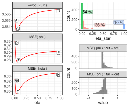
Figure 2: Model assessment for biased data example. Left column: average $-elpd$ and MSE for estimates under the SMI posterior with $\eta\in[0,1]$. Top-right: Histogram of optimal $\eta^{*}$ chosen for 1000 synthetic datasets. Bottom-Right: Histograms of differences in MSE between smi, cut and full-bayes.

5.2 Agricultural data

In our second example, we apply SMI to the agricultural dataset introduced by Styring et al., (2017), and analysed using a Cut-model. The authors test for specific agricultural practices in the first urban centres in Mesopotamia. Details of the model are given in Styring et al., (2017). We give a brief outline here with more detail in the supplement, including a graphical representation.

The observation model has a normal response, $Y$, and regression parameters, variances and random effects we collect together as a parameter vector $\psi$. It has a three-level categorical variable “manure-level” $M$ with the same dimension as $Y$. Manure-level is missing data in roughly half the observations. The generative model for the missing values in $M$ is a proportional odds model with intercept parameters $(\alpha_{1},\alpha_{2})$ and the effect $\gamma$ for a higher-level covariate, “site size”. Bayesian analysis suggests that the proportional odds module is misspecified. The parameter of scientific interest is $\gamma$; the authors test for $\gamma<0$. In our notation $M$ plays the role of $\varphi$ above, and $\gamma$ plays the role of $\theta$.

In Fig. 3 we plot density estimates for the posterior distribution of $\gamma$ at a grid of values of $\eta$. The cut posterior is at the bottom ($\eta=0$). We can see the effect of dilution (see Section 4.6) as the mean $\gamma$ drifts towards zero as $\eta$ approaches zero. The Bayesian posterior is at the top ($\eta=1$). The estimated $elpd$ is plotted as a function of $\eta$ in the top panel of Fig. 4. The $\eta$-value minimising the negative $elpd$ is 0.82. The evidence for $\gamma<0$ is much stronger at the candidate posterior as it suffers less dilution than the cut posterior. This is quantified in the lower graph in Fig. 4 where we plot the posterior odds for $\gamma<0$ against $\eta$. These odds are the Bayes Factor (BF) at $\eta=1$, because the prior for $\gamma$ is symmetric about zero. We see the evidence for $\gamma<0$ is far stronger at the selected $\eta$-value (BF=117.11) than it is at the cut-model (BF=5.54).

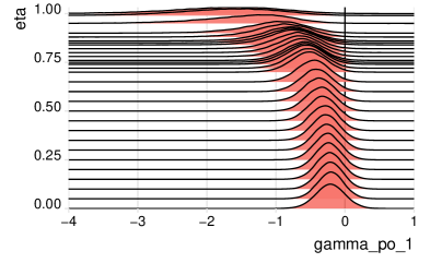
Figure 3: Posterior distribution of $\gamma$ in the PO module for different values of $\eta\in[0,1]$

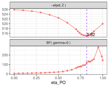
Figure 4: Top: Estimated elpd as predictive criteria for choosing the value of $\eta\in[0,1]$ The maximum is reached near to $\eta=0.8$. Bottom: The Bayes Factor for the hypothesis $H_{o}:\gamma<0$

5.3 Epidemiological data

In our final example, we apply SMI to an epidemiological dataset introduced by Maucort-Boulch et al., (2008), studying the correlation between human papilloma virus (HPV) prevalence and cervical cancer incidence, revisited by Plummer, (2015) and Jacob et al., 2017a in the context of cut vs full Bayes models.

The model has two modules: in each population $i=1,...,13$, a Poisson response for the number of cancer cases $Y_{i}$ in $T_{i}$ women-years of followup, and a Binomial model for the number $Z_{i}$ of women infected with HPV in a sample of size $N_{i}$ from the $i$’th population,

$$Y_{i}\sim Poisson(\mu_{i})$$

$$\mu_{i}=T_{i}\exp(\theta_{1}+\theta_{2}\phi_{i})$$

$$Z_{i}\sim Binomial(N_{i},\phi_{i}).$$

In Fig. 5 we show the posterior distribution for the parameters $\theta_{1},\theta_{2}$. The top panel shows posterior samples for the cut model posterior ($\eta=0$) in black and the full posterior ($\eta=1$) in yellow. The graph agrees with an equivalent plot appearing in Jacob et al., 2017a . SMI interpolates between these two distributions. The two panels at the bottom of Fig. 5 show the approximate marginal SMI posteriors for the two parameters.

Lastly, we follow Jacob et al., 2017a and evaluate the predictive performance of the various SMI candidate distributions for $\eta\in[0,1]$. Our criterion is the elpd, estimated using the WAIC, and plotted against $\eta$ in Fig. 6. Results expand on but support those reported by Jacob et al., 2017a : For the task of predicting the Binomial data, the cut model performs best (lower -elpd at $\eta=0$ on the left panel of Fig. 6). This is expected as the Poisson module is suspected of being misspecified. Eliminating contamination improves prediction of $Z$. For the task of predicting the Poisson module, full Bayesian analysis performs best (lower -elpd at $\eta=1$ in the right panel of Fig. 6) as the information contained in the Binomial data is reliable and helps correct the misspecified module.

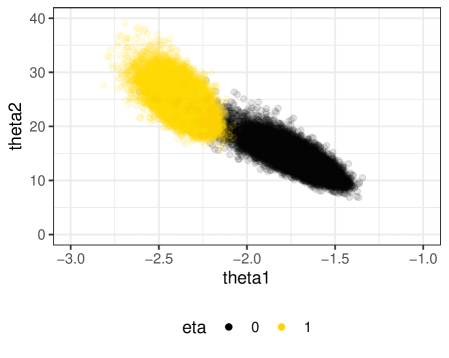
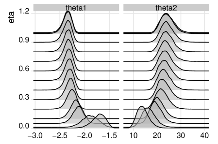
Figure 5: Joint SMI posterior for $\theta_{1}$ and $\theta_{2}$ for the HPV model using MCMC on the SMI posterior with $\eta\in[0,1]$

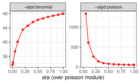
Figure 6: Estimated elpd (using $WAIC$) as predictive criteria for selection of $\eta\in[0,1]$ for the HPV model. The full model ($\eta=1$) performs better for prediction of the Poisson data, while the cut model ($\eta=0$) dominates for the Binomial.

6 Discussion

We have given an extension of Bayesian inference to a family of inference procedures indexed by an influence parameter. Our inference procedures bring together Bayesian inference and two qualitatively different inference schemes, power-posteriors and Modular inference/Cut-models, used to treat model misspecification. We show the new family is coherent and falls within the larger loss-based inference framework of Bissiri et al., (2016).

We gave a straightforward procedure for choosing the inference scheme according to an external $elpd$ criterion, which we implemented using the WAIC and LOOCV. In different examples this selects Bayesian inference, Cut-model inference and interpolating candidate distributions.

When we encounter model misspecification we may consider model elaboration to improve the fit, but we may alternatively expand the inference framework.

References

- Bernardo and Smith, (2000) Bernardo, J. M. and Smith, A. F. (2000). Bayesian Theory. Wiley Series in Probability and Statistics. John Wiley & Sons, Inc., Hoboken, NJ, USA, 3 edition.
- Bissiri et al., (2016) Bissiri, P. G., Holmes, C. C., and Walker, S. G. (2016). A general framework for updating belief distributions. Journal of the Royal Statistical Society: Series B (Statistical Methodology), 78(5):1103–1130.
- Cox, (1975) Cox, D. R. (1975). Partial likelihood. Biometrika, 62(2):269–276.
- Grünwald, (2012) Grünwald, P. (2012). The Safe Bayesian. In Bshouty, N. H., Stoltz, G., Vayatis, N., and Zeugmann, T., editors, Algorithmic Learning Theory: 23rd International Conference, ALT 2012, Lyon, France, October 29-31, 2012. Proceedings, volume 7568 LNAI, pages 169–183. Springer Berlin Heidelberg.
- Grünwald and van Ommen, (2017) Grünwald, P. and van Ommen, T. (2017). Inconsistency of Bayesian Inference for Misspecified Linear Models, and a Proposal for Repairing It. Bayesian Analysis, 12(4):1069–1103.
- Holmes and Walker, (2017) Holmes, C. C. and Walker, S. G. (2017). Assigning a value to a power likelihood in a general Bayesian model. Biometrika, 104(2):497–503.
- (7) Jacob, P. E., Murray, L. M., Holmes, C. C., and Robert, C. P. (2017a). Better together? Statistical learning in models made of modules.
- (8) Jacob, P. E., O’Leary, J., and Atchadé, Y. F. (2017b). Unbiased Markov chain Monte Carlo with couplings.
- Knuiman et al., (1998) Knuiman, M. W., Divitini, M. L., Buzas, J. S., and Fitzgerald, P. E. (1998). Adjustment for Regression Dilution in Epidemiological Regression Analyses. Annals of Epidemiology, 8(1):56–63.
- Little and Rubin, (2002) Little, R. J. A. and Rubin, D. B. (2002). Statistical Analysis with Missing Data. John Wiley & Sons, Inc., Hoboken, NJ, USA, 2nd edition.
- Liu et al., (2009) Liu, F., Bayarri, M. J., and Berger, J. O. (2009). Modularization in Bayesian analysis, with emphasis on analysis of computer models. Bayesian Analysis, 4(1):119–150.
- Lunn et al., (2009) Lunn, D., Best, N., Spiegelhalter, D., Graham, G., and Neuenschwander, B. (2009). Combining MCMC with ‘sequential’ PKPD modelling. Journal of Pharmacokinetics and Pharmacodynamics, 36(1):19–38.
- Maucort-Boulch et al., (2008) Maucort-Boulch, D., Franceschi, S., and Plummer, M. (2008). International Correlation between Human Papillomavirus Prevalence and Cervical Cancer Incidence. Cancer Epidemiology Biomarkers & Prevention, 17(3):717–720.
- Meng, (1994) Meng, X.-L. (1994). Multiple-Imputation Inferences with Uncongenial Sources of Input. Statistical Science, 9(4):538–558.
- Miller and Dunson, (2018) Miller, J. W. and Dunson, D. B. (2018). Robust Bayesian Inference via Coarsening. Journal of the American Statistical Association, pages 1–13.
- Plummer, (2015) Plummer, M. (2015). Cuts in Bayesian graphical models. Statistics and Computing, 25(1):37–43.
- Spiegelhalter et al., (2014) Spiegelhalter, D. J., Thomas, A., Best, N., and Lunn, D. (2014). OpenBUGS User Manual.
- Styring et al., (2017) Styring, A. K., Charles, M., Fantone, F., Hald, M. M., McMahon, A., Meadow, R. H., Nicholls, G. K., Patel, A. K., Pitre, M. C., Smith, A., So?tysiak, A., Stein, G., Weber, J. A., Weiss, H., and Bogaard, A. (2017). Isotope evidence for agricultural extensification reveals how the world’s first cities were fed. Nature Plants, 3(6).
- Vehtari et al., (2017) Vehtari, A., Gelman, A., and Gabry, J. (2017). Practical Bayesian model evaluation using leave-one-out cross-validation and WAIC. Statistics and Computing, 27(5):1413–1432.
- Walker and Hjort, (2001) Walker, S. and Hjort, N. L. (2001). On Bayesian consistency. Journal of the Royal Statistical Society: Series B (Statistical Methodology), 63(4):811–821.
- Watanabe, (2009) Watanabe, S. (2009). Algebraic Geometry and Statistical Learning Theory. Cambridge Monographs on Applied and Computational Mathematics. Cambridge University Press.
- Xie and Meng, (2016) Xie, X. and Meng, X.-L. (2016). Dissecting multiple imputation from a multi-phase inference perspective: what happens when God’s, imputer’s and analyst’s models are uncongenial? Statistica Sinica, 27:1485–1594.