Towards automated kernel selection in machine learning systems: A SYCL case study

Abstract

Automated tuning of compute kernels is a popular area of research, mainly focused on finding optimal kernel parameters for a problem with fixed input sizes. This approach is good for deploying machine learning models, where the network topology is constant, but machine learning research often involves changing network topologies and hyperparameters. Traditional kernel auto-tuning has limited impact in this case; a more general selection of kernels is required for libraries to accelerate machine learning research.

In this paper we present initial results using machine learning to select kernels in a case study deploying high performance SYCL kernels in libraries that target a range of heterogeneous devices from desktop GPUs to embedded accelerators. The techniques investigated apply more generally and could similarly be integrated with other heterogeneous programming systems. By combining auto-tuning and machine learning these kernel selection processes can be deployed with little developer effort to achieve high performance on new hardware.

I Introduction

Modern machine learning systems, especially deep neural networks, rely heavily on a small number of compute intensive routines including convolutions and matrix multiplication. As such, improving the performance of these routines by tuning kernel parameters can have a significant impact on the time required to train large machine learning models.

Automatic kernel selection for GPUs is a well studied area especially since the rise of GPGPU programming. Many auto-tuning techniques concentrate on achieving maximum performance for a problem with given input sizes, with the expectation that when deployed these systems will carry out computations on different data of the same sizes.

Modern machine learning research often involves training models and continually tweaking the model architecture and hyperparameters to obtain the best results. As the models keep changing, standard auto-tuning techniques are of limited use, and only come into their own when the final models are deployed. As such autotuning techniques in machine learning frameworks tend to be dynamic, doing trial runs the first time an input size is used and choosing the best for subsequent runs.

Codeplay [1] has been developing an ecosystem of libraries to accelerate machine learning using SYCL [2] and aims to provide close to optimal performance on a range of compute tasks. A typical SYCL implementation converts kernels into an intermediate representation that is bundled with the final SYCL library. Supporting many different kernel instantiations in these libraries adds complexity and a cost in terms of library size and build times.

In this paper we discuss machine learning techniques to prune the number of kernel configurations that need to be provided in a library while preserving performance, and show that simple decision processes can be used to choose the best of these kernels at runtime. The discussion is based around how these techniques apply to a matrix multiply case study provided by SYCL-DNN [3].

I-A Related work

Auto-tuners such as clTune [4] and Kernel Tuner [5] have been developed optimize heterogeneous compute kernels. These tuning systems establish the best kernel parameters for a given set of inputs, but the whole tuning process has to be run for any new inputs. This can be partially mitigated by using machine learning [6, 7] to reduce the size of the parameter space that must be searched.

Auto-tuning in this form has been applied to various problems including matrix multiplication [8, 9], convolution [10], FFTs [11] and stencils [12, 13].

II A matrix multiply case study

Figure 1: Performance of each configuration for all matrix sizes in the dataset, with configurations listed in increasing mean performance. Some configurations consistently perform poorly for any set of matrix sizes, while those that perform optimally on some sizes still perform poorly on other sizes. A few of the configurations that perform poorly on the majority of cases can be seen to perform well on a small number of specific matrix sizes.

A standard kernel tuning example is a general matrix multiply. Such a kernel often has parameters describing the tile sizes used both at a work group level for programmatically caching values, and at the work item level with values in registers. Further parameters include the vector widths used to load and store values from memory and the sizes of the work groups.

The matrix multiply kernel used in this case study is provided as part of the SYCL-DNN [3] library. SYCL [2] is a royalty-free, cross-platform parallel programming framework designed to abstract the complexity of traditional parallel programming models like OpenCL, allowing developers to use modern C++ features within kernels. In particular, C++ templates are used throughout SYCL-DNN to provide specializations for data types, tile sizes and other constants with little additional code.

In the matrix multiply kernel each work item computes a tile of the output, accumulating a given number of values in each step. This gives three compile time parameters: the two dimensions of the output tile and the size of the accumulator step. An additional two parameters describe the size of the work group, however these can be set at runtime and do not require additional kernels to be compiled.

For each of the tile sizes we considered values of 1, 2, 4 and 8, giving a total of 64 possible kernels. In addition to this we compared the following work group sizes: (1, 64), (1, 128), (8, 8), (8, 16), (8, 32), (16, 8), (16,16), (32,8), (64, 1), (128, 1); giving a total of 640 possible configurations to select from.

Such a small number of configurations allows us to brute-force the performance for a number of different matrix sizes, however this is not feasible for more general kernels that have significantly more parameters or for problems where less strict heuristics are used to limit the number of configurations. For these cases more complex tuning algorithms have been proposed, such as basin hopping and evolutionary algorithms; a good discussion of these can be found in [5].

II-A The dataset

Convolutional layers in neural network models can be computed using a matrix multiply through transformations such as the im2col and Winograd, while fully connected layers are comprised of a matrix multiply and a bias add. We extracted the sizes of matrix multiplies arising from three popular neural networks: VGG [14], ResNet [15] and MobileNet [16], giving 78, 66 and 26 combinations of matrix sizes to consider respectively (170 combinations total). For each of these sizes we ran a benchmark for each of the kernel configurations, recording the runtime of the kernel and number of flops attained over a number of iterations. The benchmark platform was an AMD R9 Nano GPU.

The full dataset is shown in Figure 1, with the relative performance of each benchmark run for every configuration, sorted by their overall mean performance. With so many different configurations it is hard to isolate any individual in the figure, but it is useful to consider the distribution of performance across the matrix sizes.

There are some configurations that perform badly for all matrix sizes, with those at the far left never achieving above 30% of the optimal performance. The configurations on the far right performed well on average, but still perform poorly on some matrix sizes. Some configurations in the middle have a low average performance, but can achieve close to optimal performance on certain sizes.

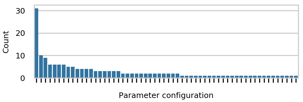
Figure 2: The number of times a configuration of kernel parameters achieves optimal performance in the dataset. One configuration is best in 32 cases, but 58 distinct configurations are best in at least one case.

Figure 2 shows that a single configuration performs best more than 3 times as often as the next best configuration, however across the full dataset there are 58 different configurations that give optimal performance for at least one set of matrix sizes. This long tail causes problems with trying to prune the number of configurations as it is hard to justify which of the configurations should be chosen to include in the selection process.

The dataset and the corresponding code is available online [17]. The machine learning routines were provided by scikit-learn [18].

II-B Determining the target number of configurations

In order to effectively deploy SYCL kernels in a library, only a restricted number of kernels can be provided without significantly inflating library size. Principal component analysis (PCA) [19, 20] can be used to help determine a good number of kernels to provide to cover the majority of cases encountered in the dataset.

PCA provides a coordinate system that concentrates the variance of the dataset in as few components as it can. By comparing the number of components required to account for a given threshold of the total variance we can estimate how many different clusters would be required to effectively encompass this variance in the dataset.

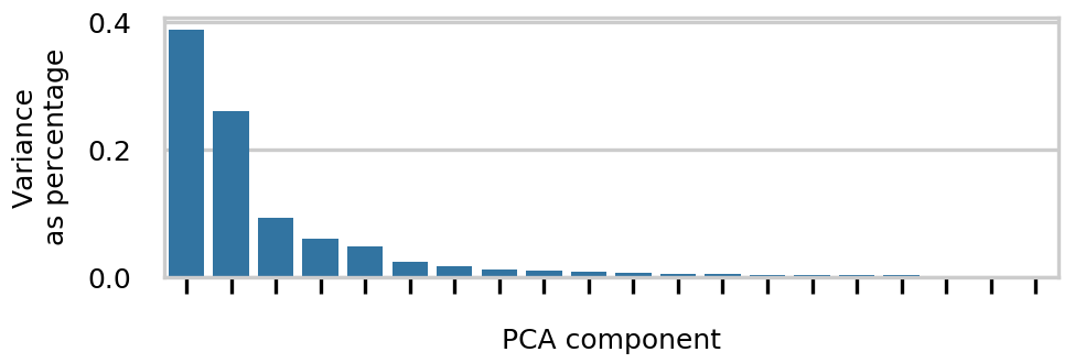
Figure 3: The percentage of the variance of the dataset accounted for by each PCA component. Over 80% of the variance is accounted for in the 4 main components, 90% is accounted for in 8 components, and 95% in 15.

Figure 3 shows the ratio of variance accounted for by each of the components identified by PCA. The first 4 components account for over 80% of the variance, 8 components account for 90% and 15 account for 95%, and so we investigate limiting the number of kernels between 4 and 15.

III Configuration pruning approaches

We compared five approaches to pruning the available kernel configurations. The simplest pruning method is choosing the top $N$ configurations that obtained optimal results.

Alongside this we compared methods of clustering the vectors of normalized performance to give a set of representatives. For each set of matrix sizes (the input features) in the dataset we have a vector of 640 normalized performance scores coming from the 640 different kernel configurations. The assumption made in this paper is that these vectors contain enough structure to provide a good basis for pruning the number of kernel configurations. Each of the following techniques uses clustering to establish a set of representatives from the dataset that exhibit different performance behavior. The kernel configurations that gives the best performance result for each of the representatives are chosen as the set of configurations to provide in the compute library.

The first clustering method evaluated is $k$-means clustering, a well known and relatively simple clustering algorithm that iteratively tries to find clusters around centroids, and the second is HDBScan [21, 22], a more complex density based clustering method. PCA can be used to reduce the dimensionality of the data and so provide a better coordinate system for $k$-means clustering, which struggles with high dimensional data. The centroids identified by $k$-means in this new coordinate system can be mapped back to the original coordinate space to give representatives of the clusters.

Finally we used a decision tree to do regression on the dataset that maps a set of matrix sizes to a vector of the expected normalized performance for each configuration. Limiting the number of leaf nodes in the decision tree ensures the tree only produces a restricted number of such vectors which are used as the cluster representatives.

III-A The results

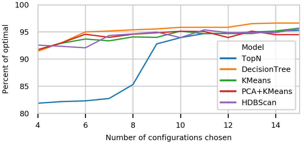
Figure 4: The performance of each pruning technique in Section III as a percentage of the optimal obtainable performance.

In order to test how well any of the following approaches generalize to unseen matrix sizes the data set was randomly segmented into a training and a test dataset of 136 and 34 elements respectively.

The different kernel configuration selection techniques were trained on the training dataset to generate a set of kernel configurations limited to a fixed upper bound. The performance of the clustering technique was measured by taking the geometric mean of the optimal result achievable given that selection for each set of matrix sizes in the test set. A score of 100% would only be obtained by selecting the best kernel for every matrix size in the test set.

The results are shown in Figure 4. When the number of configurations is very limited, the clustering methods all perform significantly better than the naive method of selecting the top kernels by count alone. With a limit of 6 kernels, the decision tree and PCA + $k$-means clustering could both achieve close to 95% of the optimal performance. As more configurations were allowed all techniques improved, achieving around 95% of the optimal performance on the test set. The decision tree consistently provided the best results when 6 or more kernel configurations were allowed, achieving 96.6% of the optimal performance in the best case.

IV Deploying the kernels

Once a set of kernels has been chosen we still need to provide a process to select which of these kernels should be run for a set of parameters. Integrating this process into a library allows the best kernel to be selected that matches the workload requested by users.

The main challenge in developing a kernel selection process is that it must balance how good the choice of kernel is with how much time it must spend in doing the selection. There is little to be gained by choosing a complex process to achieve slightly better performance if this leads to significantly more time being spent in that selection process.

Decision trees can be implemented as a series of nested if statements and so are a good target for deployment provided they do not sacrifice too much performance. To establish whether decision trees are sufficiently good at choosing kernel configurations we compare them to other classification methods that may require more computation to obtain potentially better results.

Table I shows the performance of the various classifiers tested on the dataset, which include a linear support vector machine (SVM), a radial SVM, $k$-nearest neighbors and a random forest ensemble. Despite the maximum obtainable performance achievable by the kernel configurations chosen ranging from 93% to 96.6% for different numbers of configurations, none of the models achieve over 89% performance.

The decision tree outperforms or comes close to the performance of all other classifiers, except when the model has to choose between 15 configurations. Overall the classifiers performed worse as the number of configurations grew, suggesting that the dataset is too small to correctly learn a generalization encompassing large numbers of classes.

TABLE I: The performance results for the classifiers as a percentage of the absolute optimal performance, for the kernel configurations selected by a decision tree. Note that the maximum achievable performance for the selection of configurations is limited to 92.99%, 94.98%, 95.37% and 96.61% for the 5, 6, 8 and 15 configurations respectively.

	Number of configurations
Classifier	5	6	8	15
DecisionTree	86.43	84.29	86.82	83.54
RandomForest	82.99	83.70	87.99	88.13
1NearestNeighbor	80.45	78.44	78.30	78.21
3NearestNeighbors	76.41	77.95	76.34	75.45
LinearSVM	85.88	84.17	87.96	82.50
RadialSVM	54.95	55.01	55.01	55.01

V Conclusions

In this paper we evaluated a number of general methods to prune and deploy kernel configurations in a compute library, using matrix multiply as a case study. Section III showed that clustering is effective at choosing representatives of the kernel configurations that provide good performance for a range of different input parameters. In particular the use of a decision tree consistently performed better than the other clustering methods evaluated. Section IV showed that a decision tree choosing the configuration at runtime provides very similar performance to other selection techniques while being easier to implement in the compute library, so is a good candidate to deploy in high performance libraries where low latencies are important.

This work is preliminary with two main areas that will be addressed in the future. The datasets used in this paper are fairly small, causing the models to fail to generalize which would be mitigated with larger datasets. The brute-force techniques used are infeasible for larger problems, where more intelligent parameter search methods must be used and it is unclear how well the techniques discussed here generalize to sparse data.

References

- [1] “Codeplay Software Ltd: The heterogeneous system experts,” https://codeplay.com/, accessed: 2019-11-08.
- [2] “SYCL: C++ single-source heterogeneous programming for OpenCL,” https://www.khronos.org/sycl/, accessed: 2019-03-11.
- [3] R. Burns, J. Lawson, D. McBain, and D. Soutar, “Accelerated neural networks on OpenCL devices using SYCL-DNN,” in Proceedings of the International Workshop on OpenCL, ser. IWOCL’19. New York, NY, USA: ACM, 2019, pp. 10:1–10:4. [Online]. Available: http://doi.acm.org/10.1145/3318170.3318183
- [4] C. Nugteren and V. Codreanu, “Cltune: A generic auto-tuner for opencl kernels,” in 2015 IEEE 9th International Symposium on Embedded Multicore/Many-core Systems-on-Chip, Sep. 2015, pp. 195–202.
- [5] B. van Werkhoven, “Kernel tuner: A search-optimizing gpu code auto-tuner,” Future Generation Computer Systems, vol. 90, pp. 347 – 358, 2019. [Online]. Available: http://www.sciencedirect.com/science/article/pii/S0167739X18313359
- [6] T. L. Falch and A. C. Elster, “Machine learning based auto-tuning for enhanced opencl performance portability,” in 2015 IEEE International Parallel and Distributed Processing Symposium Workshop, May 2015, pp. 1231–1240.
- [7] J. Bergstra, N. Pinto, and D. Cox, “Machine learning for predictive auto-tuning with boosted regression trees,” in 2012 Innovative Parallel Computing (InPar), May 2012, pp. 1–9.
- [8] Y. Li, J. Dongarra, and S. Tomov, “A note on auto-tuning gemm for gpus,” in Computational Science – ICCS 2009, G. Allen, J. Nabrzyski, E. Seidel, G. D. van Albada, J. Dongarra, and P. M. A. Sloot, Eds. Berlin, Heidelberg: Springer Berlin Heidelberg, 2009, pp. 884–892.
- [9] C. Nugteren, “CLBlast: A tuned OpenCL BLAS library,” in Proceedings of the International Workshop on OpenCL, ser. IWOCL ’18. New York, NY, USA: ACM, 2018, pp. 5:1–5:10. [Online]. Available: http://doi.acm.org/10.1145/3204919.3204924
- [10] B. van Werkhoven, J. Maassen, H. E. Bal, and F. J. Seinstra, “Optimizing convolution operations on gpus using adaptive tiling,” Future Generation Computer Systems, vol. 30, pp. 14 – 26, 2014, special Issue on Extreme Scale Parallel Architectures and Systems, Cryptography in Cloud Computing and Recent Advances in Parallel and Distributed Systems, ICPADS 2012 Selected Papers. [Online]. Available: http://www.sciencedirect.com/science/article/pii/S0167739X13001829
- [11] A. Nukada and S. Matsuoka, “Auto-tuning 3-d fft library for cuda gpus,” in Proceedings of the Conference on High Performance Computing Networking, Storage and Analysis, ser. SC ’09. New York, NY, USA: ACM, 2009, pp. 30:1–30:10. [Online]. Available: http://doi.acm.org/10.1145/1654059.1654090
- [12] A. Mametjanov, D. Lowell, C. Ma, and B. Norris, “Autotuning stencil-based computations on gpus,” in 2012 IEEE International Conference on Cluster Computing, Sep. 2012, pp. 266–274.
- [13] Y. Zhang and F. Mueller, “Auto-generation and auto-tuning of 3d stencil codes on gpu clusters,” in Proceedings of the Tenth International Symposium on Code Generation and Optimization, ser. CGO ’12. New York, NY, USA: ACM, 2012, pp. 155–164. [Online]. Available: http://doi.acm.org/10.1145/2259016.2259037
- [14] K. Simonyan and A. Zisserman, “Very deep convolutional networks for large-scale image recognition,” CoRR, vol. abs/1409.1556, 2014.
- [15] K. He, X. Zhang, S. Ren, and J. Sun, “Deep residual learning for image recognition,” in 2016 IEEE Conference on Computer Vision and Pattern Recognition (CVPR), June 2016, pp. 770–778.
- [16] M. Sandler, A. Howard, M. Zhu, A. Zhmoginov, and L. Chen, “Mobilenetv2: Inverted residuals and linear bottlenecks,” in 2018 IEEE/CVF Conference on Computer Vision and Pattern Recognition, June 2018, pp. 4510–4520.
- [17] “Towards automated kernel selection in macine learning systems: Supplementary code and dataset,” https://github.com/jwlawson/tuning_kernels, accessed: 2020-02-07.
- [18] F. Pedregosa, G. Varoquaux, A. Gramfort, V. Michel, B. Thirion, O. Grisel, M. Blondel, P. Prettenhofer, R. Weiss, V. Dubourg, J. Vanderplas, A. Passos, D. Cournapeau, M. Brucher, M. Perrot, and E. Duchesnay, “Scikit-learn: Machine learning in Python,” Journal of Machine Learning Research, vol. 12, pp. 2825–2830, 2011.
- [19] K. P. F.R.S., “Liii. on lines and planes of closest fit to systems of points in space,” The London, Edinburgh, and Dublin Philosophical Magazine and Journal of Science, vol. 2, no. 11, pp. 559–572, 1901. [Online]. Available: https://doi.org/10.1080/14786440109462720
- [20] M. E. Tipping and C. M. Bishop, “Probabilistic principal component analysis,” Journal of the Royal Statistical Society. Series B (Statistical Methodology), vol. 61, no. 3, pp. 611–622, 1999. [Online]. Available: http://www.jstor.org/stable/2680726
- [21] R. J. G. B. Campello, D. Moulavi, and J. Sander, “Density-based clustering based on hierarchical density estimates,” in Advances in Knowledge Discovery and Data Mining, J. Pei, V. S. Tseng, L. Cao, H. Motoda, and G. Xu, Eds. Berlin, Heidelberg: Springer Berlin Heidelberg, 2013, pp. 160–172.
- [22] L. McInnes and J. Healy, “Accelerated hierarchical density based clustering,” in 2017 IEEE International Conference on Data Mining Workshops (ICDMW), Nov 2017, pp. 33–42.