Coarsening in the two-dimensional incompressible Toner-Tu equation: Signatures of turbulence

Abstract

We investigate coarsening dynamics in the two-dimensional, incompressible Toner-Tu equation. We show that coarsening proceeds via vortex merger events, and the dynamics crucially depend on the Reynolds number Re. For low Re, the coarsening process has similarities to Ginzburg-Landau dynamics. On the other hand, for high Re, coarsening shows signatures of turbulence. In particular, we show the presence of an enstrophy cascade from the intervortex separation scale to the dissipation scale.

I Introduction

Active matter theories have made remarkable progress in understanding the dynamics of suspension of active polar particles (SPP) such as fish schools, locust swarms, and bird flocks Ramaswamy (2010); Marchetti et al. (2013); Ramaswamy (2019). The particle based Vicsek model Vicsek et al. (1995) and the hydrodynamic Toner-Tu (TT) equation Toner and Tu (1998) provide the simplest setting to investigate the dynamics of SPP. Variants of the TT equation have been used to model bacterial turbulence Wensink et al. (2012); Linkmann et al. (2019) and pattern formation in active fluids Sankararaman et al. (2004); Gowrishankar and Rao (2016); Goff et al. (2016); Husain and Rao (2017); Alert et al. (2020). An important prediction of these theories is the presence of a liquid-gas-like transition from a disordered gas phase to an orientationally ordered liquid phase Ramaswamy (2010); Cates and Tailleur (2015); Chaté (2020). This picture is dramatically altered if the density fluctuations are suppressed by imposing an incompressibility constraint. Toner and colleagues Chen et al. (2015, 2016), using dynamical renormalization group studies, showed that for the incompressible Toner-Tu (ITT) equation the order-disorder transition becomes continuous. The near ordered state of the wet SPP on a substrate or under confinement Bricard et al. (2013); Chen et al. (2016); Maitra et al. (2020) belongs to the same universality class as the two-dimensional (2D) ITT equation.

Investigating coarsening dynamics from a disordered state to an ordered state in systems showing phase transitions has been the subject of intense investigation Kibble (1980); Bray (1994); Chuang et al. (1991); Damle et al. (1996); Puri (2009); Perlekar (2019). In active matter coarsening has been studied either in systems showing motility-induced phase separation Cates and Tailleur (2015); Tiribocchi et al. (2015) or for dry aligning dilute active matter (DADAM) Chaté (2020); Mishra et al. (2010); Das et al. (2018); Katyal et al. (2020). A key challenge in understanding coarsening in DADAM comes from the fact that the density and the velocity field are strongly coupled to each other. Indeed, Ref. Mishra et al. (2010) used both the density and the velocity correlations to study coarsening in the TT equation. The authors observed that the coarsening length scale grew faster than equilibrium systems with the vector order parameter and argued that the accelerated dynamics are because of the advective nonlinearity in the TT equation. However, how nonlinearity alters energy transfer between different scales remains unanswered.

The incompressible limit, where the velocity field is the only dynamical variable, provides an ideal platform to investigate the role of advection. Therefore, in this paper, we investigate coarsening dynamics using the ITT equation Chen et al. (2016):

$$\partial_{t}\bm{u}+\lambda\bm{u}\cdot\nabla\bm{u}=-\nabla P+\nu\nabla^{2}\bm{u}+\bm{f},$$ (1)

where $\bm{u}(\bm{x},t)$ is the velocity field at position $\bm{x}$ and time $t$, $\lambda$ is the advection coefficient, $\nu$ is the viscosity, $\bm{f}\equiv\left(\alpha-\beta|\bm{u}|^{2}\right)\bm{u}$ is the active driving term with coefficients $\alpha,\beta>0$, and the pressure $P({\bm{x}},t)$ enforces the incompressibility criterion $\nabla\cdot\bm{u}=0$. We do not consider the random driving term in (1) because we are interested in coarsening under a sudden quench to zero noise. For $\lambda=0$ and in the absence of the pressure term, (1) reduces to the Ginzburg-Landau (GL) equation. On the other hand, (1) reduces to the Navier-Stokes (NS) equation on fixing $\alpha=0$, $\beta=0$, and $\lambda=1$. Since most studies of dry active matter are done on a substrate, we investigate coarsening in two space dimensions.

By rescaling $\bm{x}\to\bm{x}/L$ , $t\to\alpha t$, $\bm{u}\to\bm{u}/U$ and $P\to P/\alpha UL$, we find that the Reynolds number $\mbox{Re}=\lambda UL/\nu$ and the Cahn number $\mbox{Cn}={\ell_{c}}/L$ completely characterize the flow (see Appendix A). Here $U=\sqrt{\alpha/\beta}$ is the characteristic speed, and ${\ell_{c}}=\sqrt{\nu/\alpha}$ is the length scale above which fluctuations in the disordered state $\bm{u}=0$ are linearly unstable.

We use a pseudospectral method Perlekar and Pandit (2009); Perlekar et al. (2010) to perform direct numerical simulation (DNS) of (1) in a periodic square box of length $L$. The simulation domain is discretized with $N^{2}$ collocation points. We use a second-order exponential time differencing (ETD2) scheme Cox and Matthews (2002) for time marching. Unless stated otherwise, we set $L=2\pi$ and $N=2048$. We initialize our simulations with a disordered configuration, randomly oriented velocity vectors drawn from a Gaussian distribution with zero mean and standard deviation $\sigma=U/3$, and monitor the coarsening dynamics. Our main findings are as follows:

1. Coarsening proceeds via vortex mergers.

2. For low Re, advective nonlinearities can be ignored, and the dynamics resembles coarsening in the GL equation.

3. For high Re, we find signatures of 2D turbulence, and the coarsening accelerates with increasing Re. We also provide evidence of a forward enstrophy cascade which is a hallmark of 2D turbulence.

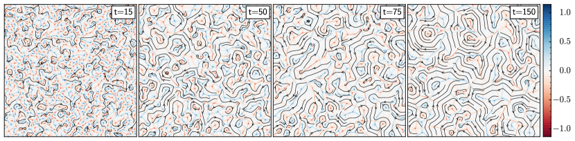
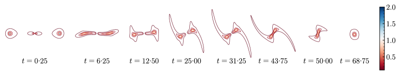
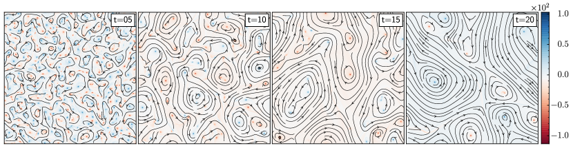
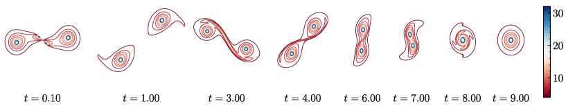
Figure 1: Pseudocolor plots of the vorticity field $\omega=\hat{z}\cdot\nabla\times\bm{u}$ superimposed on the velocity streamlines at different times for (a) $\mbox{Re}=2\pi\times 10^{2}$ and (c) $\mbox{Re}=2\pi\times 10^{4}$ in the coarsening regime. Contour plots of the vorticity field $\omega$ showing the merger of two isolated corotating vortices (vortex-saddle-vortex configuration) at (b) $\mbox{Re}=2\pi\times 10^{2}$ and (d) $\mbox{Re}=2\pi\times 10^{4}$.

In the following sections we discuss our results on the coarsening dynamics and then present conclusions in Section IV.

II Results

In the following, we quantity how the vortex dynamics controls coarsening. The pseudocolor plot of the vorticity field in Fig. 1(a) and (c) shows different stages of coarsening at low $\mbox{Re}=2\pi\times 10^{2}$ and high $\mbox{Re}=2\pi\times 10^{4}$. During coarsening, vortices merge and the inter-vortex spacing continues increasing. For low $\mbox{Re}=2\pi\times 10^{2}$ [see Fig. 1(a)], the dynamics in the coarsening regime resembles defect dynamics in the Ginzburg-Landau equation Bray (1994); Onuki (2002); Puri (2009). On the other hand, for high $\mbox{Re}=2\pi\times 10^{4}$, vorticity snapshots resemble 2D turbulence. In particular, similar to vortex merger events in 2D Meunier et al. (2005); Dizès and Verga (2002); Leweke et al. (2016); Swaminathan et al. (2016), it is easy to identify a pair of corotating vortices undergoing a merger and the surrounding filamentary structure. Earlier studiesNielsen et al. (1996); Kevlahan and Farge (1997); Swaminathan et al. (2016) on the vortex merger in two-dimensional Navier-Stokes equations showed that the filamentary structures formed during the merger process lead to an enstrophy cascade. Because the ITT equation structure is similar to NS equations, we expect that the vortex merger at high Re will also lead to an enstrophy cascade.

To further investigate the vortex merger, we perform DNS of the isolated vortex-saddle-vortex configuration at various Reynolds numbers. For these simulations we use $N=4096$ collocation points. Furthermore, to minimize the effect of periodic boundaries, we set $\alpha=-10$ for $r>0.9L/2$ and keep $\alpha=1$ otherwise, where $r\equiv\sqrt{(x-L/2)^{2}+(y-L/2)^{2}}$. This ensures that the velocity decays to zero for $r\geq 0.9L/2$. Note that a vortex in the 2D ITT equation is a point defect with unit topological charge and core radius ${\ell_{c}}$ (see Appendix B).

We observe that during the evolution of a vortex-saddle-vortex configuration [see Fig. 1(b) and (d)]: (i) similar to defect dynamics in the GL equation Yurke et al. (1993); Chaikin and Lubensky (1998); Onuki (2002), each vortex gets attracted to the saddle due to the opposite topological charge, (ii) the two vortices rotate around each other, similar to convective merging in NS Swaminathan et al. (2016); Leweke et al. (2016), and (iii) the flexure of the vortex trajectory depends on Re (see Appendix C). Thus, a vortex merger event in the two-dimensional ITT equation has ingredients from both the NS and GL equations. In Appendix C, we provide a more detailed investigation of the vortex merger with varying Re.

To quantify coarsening dynamics, we conduct a series of high-resolution DNSs ($N=2048$) of the ITT equation by varying Re while keeping $\mbox{Cn}=1/(100L)$ fixed. For ensemble averaging, we evolve $48$ independent realizations at every Re. We monitor the evolution of the energy spectrum $E_{k}(t)\equiv\frac{1}{2}\sum_{k-1/2\leq p<k+1/2}\langle|\hat{\bm{u}}_{\bm{p}}(t)|^{2}\rangle$, and the energy dissipation rate (or equivalently the excess free energy) $\epsilon(t)\equiv\left<2\nu\sum_{k}k^{2}E_{k}(t)\right>$. Here $\hat{\bm{u}}_{\bm{k}}(t)\equiv\sum_{\bm{x}}\bm{u}(\bm{x},t)\exp(-i\bm{k}\cdot\bm{x})$, $i=\sqrt{-1}$, and the angular brackets indicate the ensemble average .

II.1 Energy Dissipation Rate

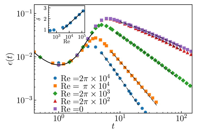
Figure 2: Plot of the energy dissipation rate $\epsilon(t)$ vs time at various Reynolds numbers. The early time evolution of $\epsilon(t)$ is well approximated by (2) (solid black line). At late times, $\epsilon(t)$ decays as $\epsilon(t)\sim t^{-\delta}\ln(t)$ (black solid lines), with $\delta$ obtained using a least-squares fit. Inset: Plot of Re vs $\delta$ and the fit $\delta\sim-2.71+0.46\ln(\mbox{Re})$ for $\mbox{Re}>>1$. For $\mbox{Re}\rightarrow 0$, consistent with Ginzburg-Landau scaling, we obtain $\delta\to 1$.

The time evolution of the energy dissipation rate $\epsilon(t)$ is shown in Fig. 2. For the initial disordered configuration, because the statistics of velocity separation is Gaussian, we approximate the fourth-order correlations in terms of the product of second-order correlations to get the following equation for the early time evolution of the energy spectrum Bratanov et al. (2015):

$$\partial_{t}E_{k}(t)\approx[2\alpha-8\beta E(t)]E_{k}(t)-2\nu k^{2}E_{k}(t),$$ (2)

where $E(t)=\sum_{k}E_{k}(t)$. In Fig. 2 we show that the early-time evolution of the energy dissipation rate $\epsilon(t)$ obtained from (2) is in good agreement with the DNS.

For late times, coarsening proceeds via vortex (defect) mergers. For GL equations in two dimensions, Refs. Yurke et al. (1993); Qian and Mazenko (2003) show that $\epsilon(t)\propto t^{-1}\ln(t)$. In our simulations, we find that $\epsilon(t)\propto t^{-\delta}\ln(t)$, where $\delta$ is now Re dependent. For low Re, where the effect of the advective nonlinearity can be ignored, we recover GL scaling ($\delta\rightarrow 1$ as $\mbox{Re}\rightarrow 0$). For high Re, coarsening dynamics is accelerated with $\delta\sim-2.71+0.46\ln(\mbox{Re})$ [see Fig. 2, inset].

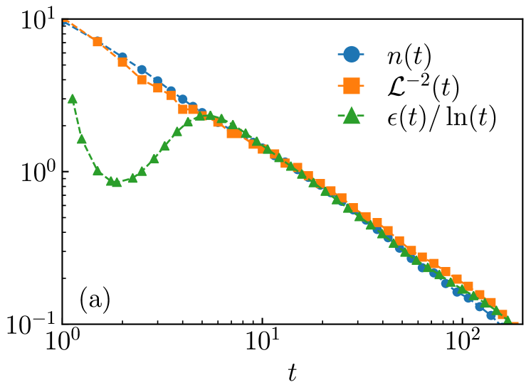
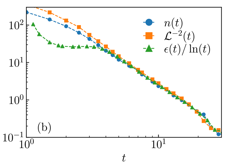
Figure 3: Plots comparing the time evolution of $n(t)$, $\mathcal{L}(t)$, and $\epsilon(t)$ for (a) $\mbox{Re}=2\pi\times 10^{2}$, and (b) $\mbox{Re}=2\pi\times 10^{4}$. The curves are vertically shifted to highlight identical scaling behavior [$n(t)\propto\mathcal{L}^{-2}(t)\propto\epsilon(t)\ln(t)\propto t^{-\delta}$] in the coarsening regime.

II.1.1 Energy dissipation rate and the coarsening length scale

We now discuss the relationship between the energy dissipation rate, the defect number density, and the coarsening length scale. The coarsening length scale Onuki (2002); Puri (2009); Perlekar et al. (2014, 2017); Perlekar (2019)

$$\mathcal{L}(t)\equiv 2\pi\frac{\sum_{k}E_{k}(t)}{\sum_{k}kE_{k}(t)}$$ (3)

has been used to monitor inter-defect separation during the dynamics.

We identify defects from the local minima of the $|{\bm{u}}|$ field in our DNS of the ITT equation and define the defect number density as $n(t)\equiv{\cal N}_{d}(t)/L^{2}$, where ${\cal N}_{d}$ denotes the number of defects at time $t$ . In Fig. 3, we show that in the coarsening regime $n(t)\propto\mathcal{L}^{-2}(t)\propto\epsilon(t)/\ln(t)$ for low $\mbox{Re}=2\times 10^{2}$ as well as high $\mbox{Re}=2\times 10^{4}$. As discussed above, the energy dissipation rate decays as $\epsilon(t)\sim t^{-\delta}\ln(t)$ in the coarsening regime. Similar to GL dynamics, we find that $n(t)\propto\mathcal{L}^{-2}(t)$ even for the ITT equation. However, both $n(t)$ and $\mathcal{L}^{-2}(t)$ show a power-law decay ($n\propto{\mathcal{L}}^{-2}\sim t^{-\delta}$) without any logarithmic correction.

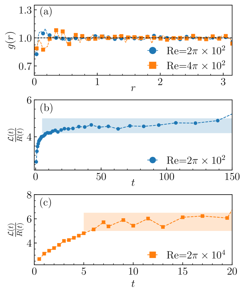
Figure 4: (a) Plot of the radial distribution function $g(r)$ for $\mbox{Re}=2\pi\times 10^{2}$ at time $t=40$ and $\mbox{Re}=2\pi\times 10^{4}$ at time $t=10$ in the coarsening regime. The dashed black line indicates theoretical prediction $g(r)=1$ for uniformly distributed points. Plots showing $\mathcal{L}(t)/R(t)$ for (b) $\mbox{Re}=2\pi\times 10^{2}$ and (c) $\mbox{Re}=2\pi\times 10^{4}$. $\mathcal{L}(t)/R(t)$ is fairly constant in the coarsening regime (shaded region).

A purely geometrical argument can be constructed to explain the observed relation between $n(t)$ and $\mathcal{L}(t)$. As we start our simulations from a disordered configuration, defects are expected to be uniformly distributed over the entire simulation domain. In Fig. 4(a), we plot the radial distribution function Allen and Tildesley (2017)

$$g(r)\equiv\frac{1}{2\pi rdrn(t)}\sum_{i\neq j}\delta(r-r_{ij}).$$ (4)

Here $r_{ij}=|\bm{r}_{i}-\bm{r}_{j}|$, $\bm{r}_{i}$ are the defect coordinates and $dr$ is the bin width used to calculate $g(r)$. Consistent with our assumption above, we find $g(r)=1$, indicating defects are uniformly distributed in the coarsening regime. Then following Refs. Chandrasekhar (1943); Hertz (1909) we get $R(t)=1/2\sqrt{n(t)}$, where $R(t)$ is the average nearest-neighbor distance at time $t$. Consistent with the dynamic scaling hypothesis Bray (1994), in Fig. 4(b) and (c) we show that ${\mathcal{L}}(t)\propto R(t)$ in the coarsening regime. Using this, we get ${\mathcal{L}}(t)\propto 1/\sqrt{n(t)}$ independent of Re.

For systems with topological defects, the energy dissipation rate (or the excess free energy) is proportional to the defect number density $n(t)$ Bray (1994); Chaikin and Lubensky (1995, 1998); Yurke et al. (1993); Qian and Mazenko (2003). Thus, consistent with Fig. 3, we get ${\cal L}(t)\propto 1/\sqrt{\epsilon(t)}$ (apart from the logarithmic factor).

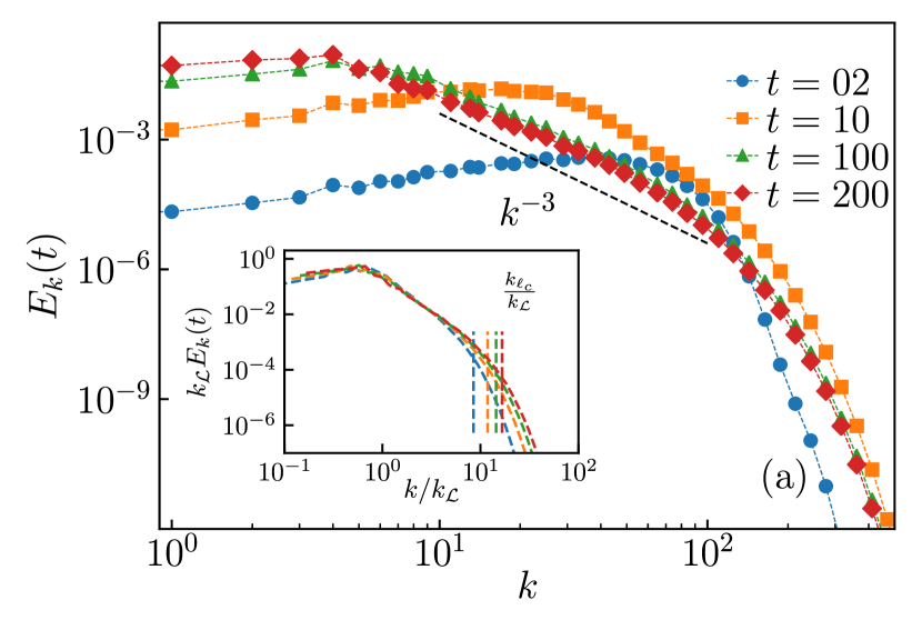
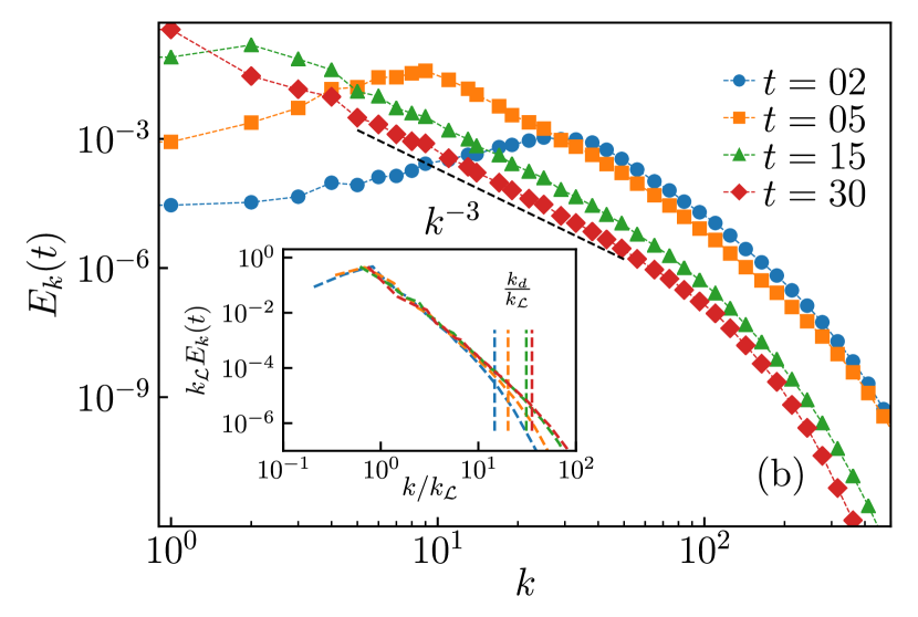
Figure 5: Time evolution of the energy spectra for (a) $\mbox{Re}=2\pi\times 10^{2}$, and (b) $\mbox{Re}=2\pi\times 10^{4}$. Inset: The scaled energy spectrum $k_{\mathcal{L}}E_{k}(t)$ versus $k/k_{\mathcal{L}}$ shows an excellent collapse between wave numbers $k_{\mathcal{L}}$ and $k_{\ell_{c}}(k_{d})$ for $\mbox{Re}=2\pi\times 10^{2}$ ($\mbox{Re}=2\pi\times 10^{4}$), confirming the dynamical scaling hypothesis. The wave numbers $k_{\ell_{c}}$ and $k_{d}$ at different times are marked by vertical dashed lines (same colors as the spectra).

II.2 Energy spectrum

The plots in Fig. 5(a) and (b) show the energy spectrum $E_{k}(t)$ versus $k$ at different times for low $\mbox{Re}=2\pi\times 10^{2}$ and high $\mbox{Re}=2\pi\times 10^{4}$. In both cases, the energy spectrum in the coarsening regime shows a power-law scaling $E_{k}(t)\propto k^{-3}$. We find that consistent with the dynamic scaling hypothesis Bray (1994), the scaled spectrum collapses between wave numbers $k_{\mathcal{L}}\equiv 1/\mathcal{L}$ and $k_{\ell_{c}}\equiv\ell_{c}^{-1}$ for low Re. At high Re the collapse is between $k_{\mathcal{L}}$ and the dissipation wave number $k_{d}$ [see insets in Fig. 5(a) and (b)].

The observed $k^{-3}$ scaling for the energy spectrum can appear because of (i) the modulation of the velocity field around the topological defects (Porod’s tail) Onuki (2002) and (ii) the enstrophy cascade, similar to two-dimensional turbulence, due to the advective nonlinearity in (1).

II.3 Enstrophy Budget

To investigate the dominant balances between different scales, we use the scale-by-scale enstrophy budget equation

$$\partial_{t}\Omega_{k}(t)+T_{k}(t)=-2\nu k^{2}\Omega_{k}(t)+{\mathcal{F}}_{k}(t),$$ (5)

where $\Omega_{k}\equiv k^{2}E_{k}$ is the enstrophy, $\mathcal{F}_{k}(t)\equiv k^{2}(\hat{\bm{u}}_{-k}\cdot\hat{\bm{f}}_{k}+\hat{\bm{u}}_{k}\cdot\hat{\bm{f}}_{-k})$ is the net enstrophy injected because of active driving, $T_{k}\equiv dZ_{k}(t)/dt$ is the enstrophy transfer function, and $Z_{k}\equiv\sum_{|\bm{p}|\leq|{\bm{k}}|}^{N/2}\hat{\omega}_{\bm{p}}\cdot\widehat{(\bm{u}\cdot\nabla\omega)}_{-\bm{p}}$ is the enstrophy flux.

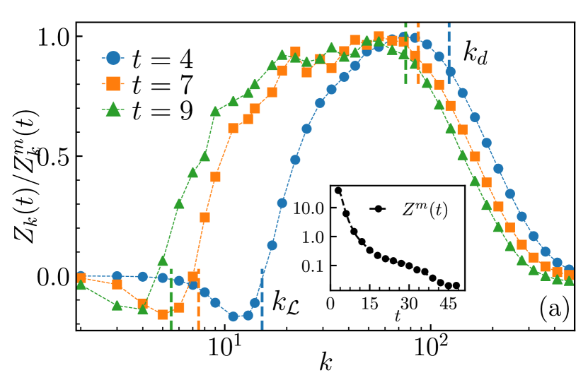
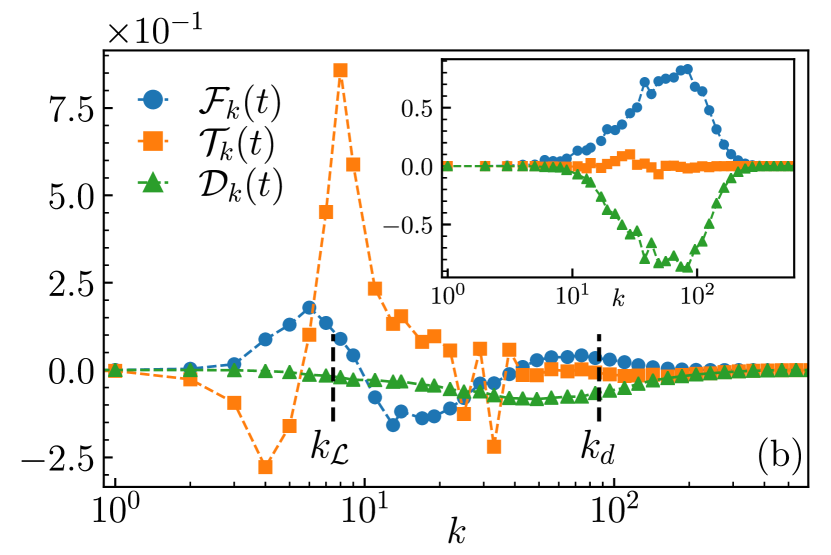
Figure 6: (a) Plot of the enstrophy flux $Z_{k}(t)/Z^{m}(t)$ versus $k$ at $\mbox{Re}=2\pi\times 10^{4}$ for different times in the coarsening regime. Wave numbers $k_{\mathcal{L}}$ and ${k_{d}}$ are marked with vertical dashed lines (same colors as the main plot). Inset: Time evolution of $Z^{m}(t)$. (b) Enstrophy budget: Plot of the transfer function ${\mathcal{T}}_{k}\equiv dZ_{k}/dk$, enstrophy injection due to the active driving ${\mathcal{F}}_{k}$, and the enstrophy dissipation $\mathcal{D}_{k}=-2\nu k^{2}\Omega_{k}$ for $\mbox{Re}=2\pi\times 10^{4}$ and at time $t=7$ in the coarsening regime. Inset: Plot of different terms in the enstrophy budget for low $\mbox{Re}=2\pi\times 10^{2}$ and at time $t=25$ in the coarsening regime.

The classical theory of 2D turbulence Kraichnan (1967); Leith (1968); Batchelor (1969); Pandit et al. (2009); Boffetta and Ecke (2012); Pandit et al. (2017) assumes the presence of an inertial range with constant enstrophy flux at scales smaller than the forcing scale and larger than the dissipation scale. Indeed, for high $\mbox{Re}=2\pi\times 10^{4}$, in Fig. 6(a) we confirm the presence of a positive enstrophy flux $Z_{k}$ between wave number $k_{\mathcal{L}}\equiv 1/{\mathcal{L}}$, corresponding to the intervortex, separation and the dissipation wave number $k_{d}\equiv{\left({8\nu^{3}}/{Z^{m}}\right)}^{-1/6}$ for $2\leq t<30$ in the coarsening regime. As the coarsening proceeds, the region of positive flux becomes broader, and $k_{\mathcal{L}}$ shifts to smaller wave numbers, but the maximum value of the flux $Z^{m}(t)$ decreases [Fig. 6(a), inset]. In Fig. 6(b) we plot different terms in the enstrophy budget equation (5). We find that the active driving primarily injects enstrophy (${\mathcal{F}}_{k}>0$) around wave number $k_{\mathcal{L}}$ but, unlike classical turbulence, it is not zero in the region of constant enstrophy flux ($k_{\mathcal{L}}<k<k_{d}$). Viscous dissipation is active only at small scales $k\geq k_{d}$. At late times $t>30$, the enstrophy flux is negligible [Fig. 6(a,inset)].

For low Re, the enstrophy transfer $T_{k}$ is negligible, and the enstrophy dissipation $\mathcal{D}_{k}(t)$ balances the injection because of the active driving ${\mathcal{F}}_{k}(t)$ [see Fig. 6(b), inset]. Therefore, the $k^{-3}$ scaling in the energy spectrum [Fig. 5(a)] is due to Porod’s tail.

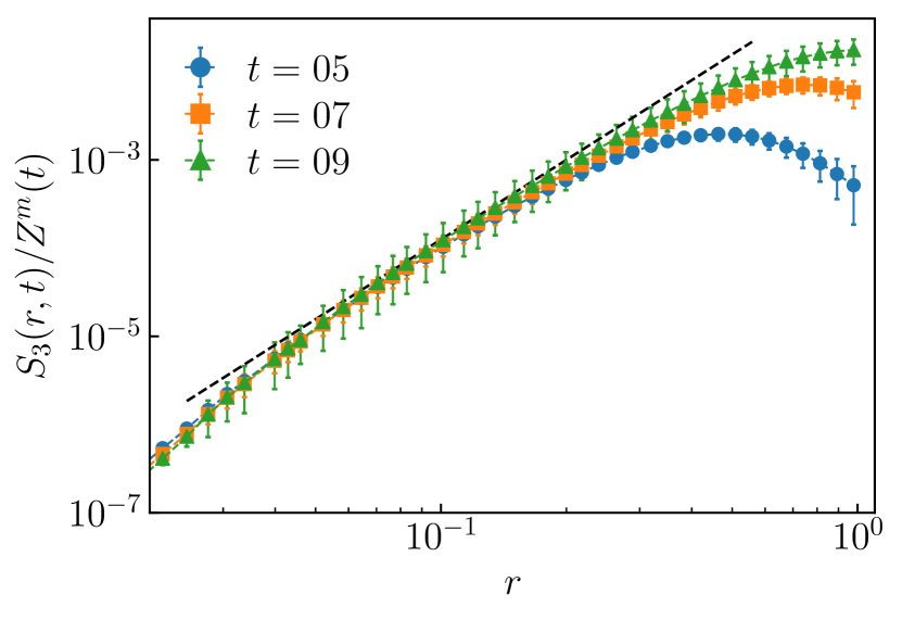
Figure 7: Plot of the third-order velocity structure function $S_{3}(r,t)$ scaled by the maxima of enstrophy flux $Z^{m}(r)$ for $t=5-9$ in the coarsening regime. The dashed black line shows the theoretical prediction $S_{3}(r)/Z^{m}(t)=\frac{1}{8}r^{3}$ for comparison.

II.4 Third-order Velocity Structure Function

The real-space indicator of the enstrophy flux in 2D turbulence is the following exact relation for the third-order velocity structure function:

$$S_{3}(r,t)=\frac{1}{8}Z_{k\sim 1/r}r^{3}.$$ (6)

Here $S_{3}(r,t)\equiv\langle\left[\delta_{r}u\right]^{3}\rangle$, $\delta_{r}u\equiv\left[\bm{u}(\bm{x}+\bm{r},t)-\bm{u}(\bm{x},t)\right].\hat{\bm{r}}$, and the angular brackets indicate spatial and ensemble averaging Cerbus and Chakraborty (2017); Lindborg (1996). In the statistically steady turbulence, the enstrophy flux $Z_{k}$ is constant in the inertial range and is equal to the enstrophy dissipation rate. During coarsening in ITT, we observe a nearly uniform flux $Z_{k}$ for $k_{\mathcal{L}}\leq k\leq k_{d}$, albeit with decreasing magnitude [see Fig. 6(a)]. Therefore, for ITT we choose $Z_{k\sim 1/r}=Z^{m}(t)$ in (6). In Fig. 7, we show the compensated plot of $S_{3}(r,t)$ in the coarsening regime and find the inertial range scaling to be consistent with the exact result (6).

II.5 Effect of noise on the coarsening dynamics

To investigate the effect of noise on the coarsening dynamics, we add a Gaussian noise ${{\bm{\eta}}({\bm{x}},t)}$ to the ITT equation Chen et al. (2016),

$$\partial_{t}\bm{u}+\lambda\bm{u}\cdot\nabla\bm{u}=-\nabla P+\nu\nabla^{2}\bm{u}+\bm{f}+\bm{\eta},$$ (7)

where $\left<{{\bm{\eta}}(\bm{x},t)}\right>=0$ and $\left<\eta_{i}(\bm{x},t)\eta_{j}(\bm{x}^{\prime},t^{\prime})\right>=A\delta_{ij}\bm{\delta}(\bm{x}-\bm{x}^{\prime})\delta(t-t^{\prime})$, where $A$ controls the noise strength. In Fig. 8, we show that the evolution of the energy dissipation rate $\epsilon(t)$ for $\mbox{Re}=2\pi\times 10^{4}$, averaged over $16$ independent noise realizations, remains unchanged for different values of $A=0,0.1,$ and $0.01$. Clearly, the presence of noise in the ITT equation does not alter the coarsening dynamics.

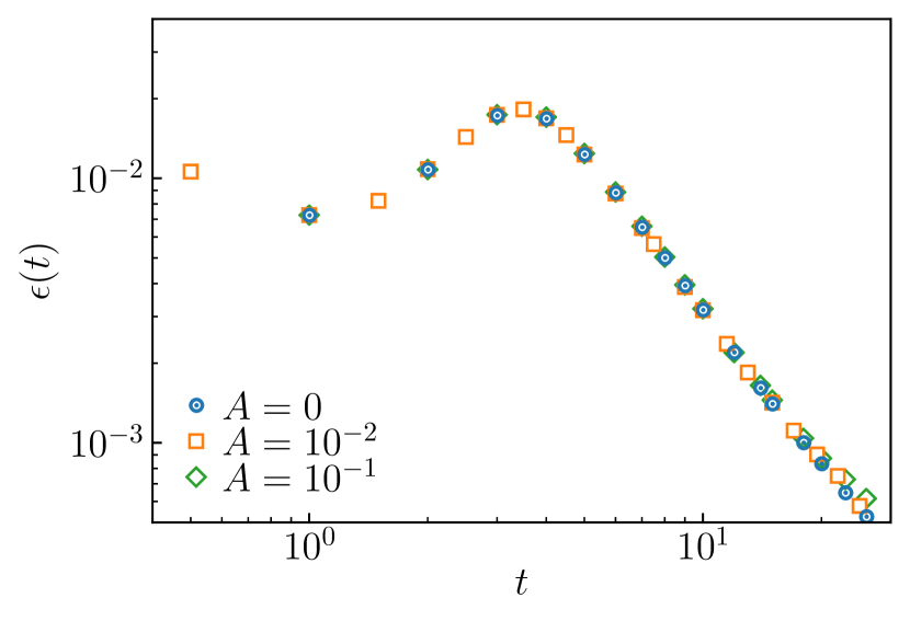
Figure 8: Plot comparing the evolution of the energy dissipation rate at different noise strengths for $\mbox{Re}=2\pi\times 10^{4}$. For ensemble averaging, we evolve 16 independent realizations at $A=10^{-1}$ and $A=10^{-2}$.

III Coarsening in ITT versus bacterial turbulence

Bacterial turbulence (BT) refers to the chaotic spatiotemporal flows generated by dense suspensions of motile bacteria Dombrowski et al. (2004); Wensink et al. (2012). The dynamics of a turbulent bacterial suspension is modeled by the ITT equation, albeit with the viscous dissipation in ITT replaced with a Swift-Hohenberg-type fourth-order term to mimic energy injection due to bacterial swimming Dunkel et al. (2013); Wensink et al. (2012); Bratanov et al. (2015); Linkmann et al. (2019, 2020),

$$\partial_{t}{\bm{u}}+\lambda{\bm{u}}\cdot\nabla{\bm{u}}=-\nabla P-\nu\nabla^{2}{\bm{u}}+\Gamma\nabla^{4}{\bm{u}}+{\bm{f}},$$ (8)

where $\nu>0$ and the parameter $\Gamma>0$.

In contrast to BT (8) , the ITT is a model of flocking dynamics. Indeed the homogeneous, ordered state is a stable solution of the ITT (1) but not of BT (8). Furthermore, (8) and its variants show an inverse energy transfer from small scales to large scales, whereas during coarsening in ITT we observe a forward enstrophy cascade from the coarsening length scale ${\mathcal{L}}$ to small scales.

IV Conclusion

In conclusion, we have investigated coarsening dynamics in ITT equations. We find that at low Reynolds number the dynamics is similar to coarsening in the Ginzburg-Landau equation, whereas for high Reynolds numbers coarsening shows signatures of 2D turbulence. Specifically, for high Reynolds numbers, we showed the presence of an enstrophy cascade which accelerates the coarsening dynamics and verified the exact relation for the structure function. Our results would also be experimentally relevant to a dense suspension of active polar particles that undergo a flocking transition, such as suspensions of active polar rods Kudrolli et al. (2008); Kumar et al. (2014).

Appendix A Dimensionless ITT equation

Consider the incompressible Toner-Tu (ITT) equation

$$\partial_{t}\bm{u}+\lambda\bm{u}\cdot\nabla\bm{u}=-\nabla P+\nu\nabla^{2}\bm{u}+\left(\alpha-\beta|\bm{u}|^{2}\right)\bm{u}.$$

By rescaling the space ${\bm{x}^{\prime}}\to{\bm{x}}/L$, the time $t^{\prime}\to\alpha t$, the pressure $P^{\prime}\rightarrow{P}/{\alpha LU}$, and the velocity field $\bm{u^{\prime}}\to\bm{u}/U$, the ITT equation becomes

$$\alpha U\partial_{t^{\prime}}{\bm{u^{\prime}}}+\frac{\lambda U^{2}}{L}\bm{u^{\prime}}\cdot\nabla^{\prime}\bm{u^{\prime}}=-\alpha U\nabla^{\prime}P^{\prime}+\frac{\nu U}{L^{2}}\nabla^{\prime 2}\bm{u^{\prime}}$$

$$+\left(\alpha-\beta U^{2}|\bm{u^{\prime}}|^{2}\right)U\bm{u^{\prime}},$$

where $U^{2}=\alpha/\beta$. Ignoring the primed index for convenience, we arrive at the dimensionless form of the ITT equation:

$$\partial_{t}\bm{u}+\mbox{Re}\mbox{Cn}^{2}\bm{u}\cdot\nabla\bm{u}=-\nabla P+\mbox{Cn}^{2}\nabla^{2}\bm{u}+\left(1-|\bm{u}|^{2}\right)\bm{u}.$$

Here $\mbox{Re}\equiv\lambda LU/\nu$ is the Reynolds number, $\mbox{Cn}\equiv{{\ell_{c}}}/{L}$ is the Cahn number, and ${\ell_{c}}=\sqrt{\nu/\alpha}$ is the length scale above which fluctuations in the homogeneous disordered state ${\bm{u}}=0$ are linearly unstable.

Appendix B Vortex Solution

Consider the radially symmetric velocity field of an isolated unbounded vortex ${\bm{u}}({\bm{x}},t)\equiv f(r)\hat{\theta}$, where $\hat{\theta}$ is the unit vector along the angular direction, $f(0)=0$, and $f^{\prime}(1)=0$. Substituting in the ITT equation, we get the following equations:

$$\left(f^{\prime\prime}+\frac{f^{\prime}}{r}-\frac{f}{r^{2}}\right) = \frac{1}{\mbox{Cn}^{2}}(f^{2}-1)f,$$ (9)

$$P = \mbox{Re}\mbox{Cn}^{2}\int_{0}^{r}\frac{f^{2}(r^{\prime})}{r^{\prime}}dr^{\prime},$$ (10)

where the prime indicates the derivative with respect to $r$. Note that (9) does not depend on Re and is identical to the equation of a defect in the Ginzburg-Landau equation Onuki (2002). In Fig. 9 we plot the numerical solution of $f(r)$ for different values of Cn. For $\mbox{Cn}<<1$, a regular perturbation analysis reveals that $f(r)\to Ar(1-r^{2}/8\mbox{Cn}^{2})$.

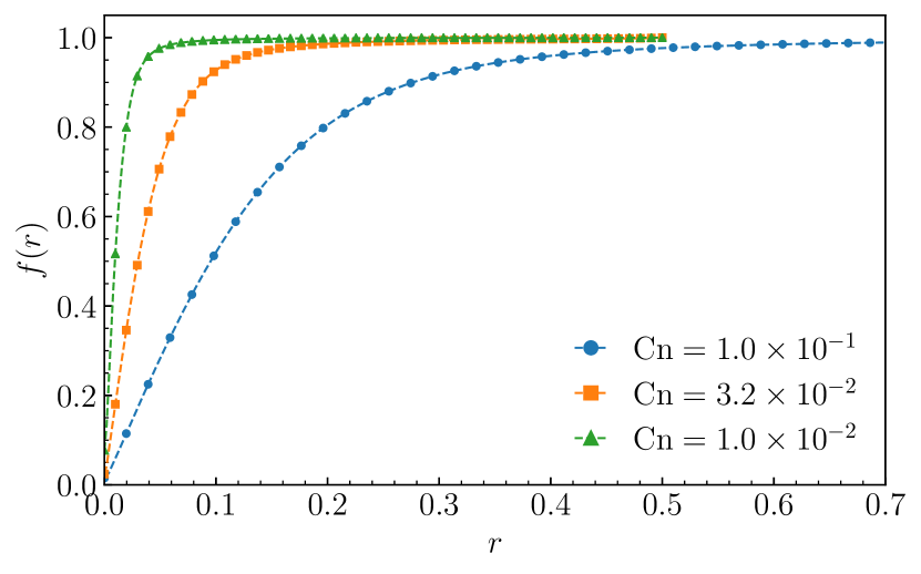
Figure 9: Plot of $f(r)$ vs $r$ for different values of Cn.

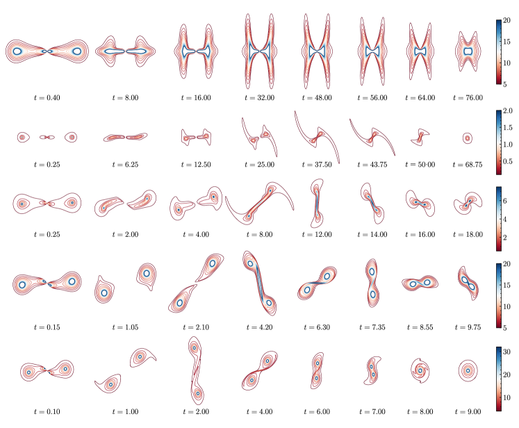
Figure 10: (a)-(e) Contour plots of the vorticity field $\omega$ at various times during the merger process for different values of the Reynolds number $\mbox{Re}=0,\,2\pi\times 10^{2},\,2\pi\times 10^{3},\,\pi\times 10^{4},\,\rm{and}\;2\pi\times 10^{4}$.

Appendix C Vortex Merger Dynamics

To investigate the merger of two corotating vortices, we perform a DNS of an isolated vortex-saddle-vortex configuration at various Reynolds numbers. We use a square domain of area $L^{2}=4\pi^{2}$ and discretize it with $N^{2}=4096^{2}$ collocation points. Furthermore, to minimize the effect of periodic boundaries, we set $\alpha=-10$ for $r>0.9L/2$ and keep $\alpha=1$ otherwise, where $r\equiv\sqrt{(x-L/2)^{2}+(y-L/2)^{2}}$. This ensures that the velocity decays to zero for $r\geq 0.9L/2$. The initial condition constitutes a saddle at the center of the square domain and two vortices placed at coordinates $[(L-1)/2,L/2]$ and $[(L+1)/2,L/2]$. As discussed in the main text, it is important to note that (i) similar to the GL equation Yurke et al. (1993); Onuki (2002), vortices in ITT have a topological charge and (ii) similar to the NS equation Doering and Gibbon (1995), the ITT equation has an advective nonlinearity and the presence of pressure leads to nonlocal interactions.

In Fig. 10(a)-(e), we plot vorticity contours during different stages of the vortex merger for different Re. Since the saddle is at an equal distance away from the two vortices, its position does not change during evolution. For low $\mbox{Re}=0$, the vortex dynamics has similarities to the overdamped motion of defects with opposite topological charge in the Ginzburg-Landau equation. Vortices get attracted to the saddle and move along a straight-line path. On increasing $\mbox{Re}\geq 2\pi\times 10^{2}$, similar to Navier-Stokes, advective nonlinearity in the ITT becomes crucial. Not only are the vortices attracted to the saddle, but they also go around each other.

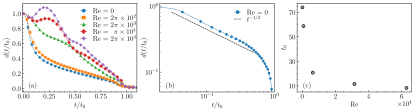
Figure 11: (a) Plot of inter vortex distance $d(t)$ vs time $t$ at various Reynolds numbers. The time axis is scaled by the merger time $t_{0}$. (b) Log-log plot of $d(t)$ vs $t$ for $\mbox{Re}=0$; the black dashed line shows the $1/\sqrt{t}$ scaling. (c) Plot of merger time $t_{0}$ versus Re. As Re increases, merger time decreases.

In Fig. 11(a) we plot the intervortex separation $d(t)$ versus time for different Re. Because of long-range hydrodynamic interactions due to incompressibility, the merger dynamics is accelerated even for $\mbox{Re}=0$. The intervortex separation decreases as $d(t)\sim 1/\sqrt{t}$ [see Fig. 11(b)], in contrast to the much slower $d(t)\sim\sqrt{t_{0}-t}$ observed in the GL dynamics Chaikin and Lubensky (1995); Denniston (1996). On increasing the Re number, inertia becomes dominant, vortices rotate around each other, and $d(t)$ decreases in an oscillatory manner. The time for the merger $t_{0}$ decreases with increasing Re [see Fig. 11(c)].

References

- Ramaswamy (2010) S. Ramaswamy, Annu. Rev. Condens. Matter Phys. 1, 323 (2010).
- Marchetti et al. (2013) M. C. Marchetti, J. F. Joanny, S. Ramaswamy, T. B. Liverpool, J. Prost, M. Rao, and R. A. Simha, Rev. Mod. Phys. 85, 1143 (2013).
- Ramaswamy (2019) S. Ramaswamy, Nat. Rev. Phys. 1, 640 (2019).
- Vicsek et al. (1995) T. Vicsek, A. Czirók, E. Ben-Jacob, I. Cohen, and O. Shochet, Phys. Rev. Lett. 75, 1226 (1995).
- Toner and Tu (1998) J. Toner and Y. Tu, Phys. Rev. E 58, 4828 (1998).
- Wensink et al. (2012) H. H. Wensink, J. Dunkel, S. Heidenreich, K. Drescher, R. E. Goldstein, H. Lowen, and J. M. Yeomans, PNAS 109, 14308 (2012).
- Linkmann et al. (2019) M. Linkmann, G. Boffetta, M. C. Marchetti, and B. Eckhardt, Phys. Rev. Lett. 122, 214503 (2019).
- Sankararaman et al. (2004) S. Sankararaman, G. I. Menon, and P. B. Sunil Kumar, Phys. Rev. E 70, 031905 (2004).
- Gowrishankar and Rao (2016) K. Gowrishankar and M. Rao, Soft Matter 12, 2040 (2016).
- Goff et al. (2016) T. L. Goff, B. Liebchen, and D. Marenduzzo, Phys. Rev. Lett. 117, 238002 (2016).
- Husain and Rao (2017) K. Husain and M. Rao, Phys. Rev. Lett. 118, 078104 (2017).
- Alert et al. (2020) R. Alert, J.-F. Joanny, and J. Casademunt, Nature Physics 16, 682 (2020).
- Cates and Tailleur (2015) M. E. Cates and J. Tailleur, Annu. Rev. Condens. Matter Phys. 6, 219 (2015).
- Chaté (2020) H. Chaté, Annu. Rev. Condens. Matter Phys. 11, 189 (2020).
- Chen et al. (2015) L. Chen, C. F. Lee, and J. Toner, New J. Phys. 17, 042002 (2015).
- Chen et al. (2016) L. Chen, C. F. Lee, and J. Toner, Nat. Comm. 7, 12215 (2016).
- Bricard et al. (2013) A. Bricard, J.-B. Caussin, N. Desreumaux, O. Dauchot, and D. Bartolo, Nature 503, 95 (2013).
- Maitra et al. (2020) A. Maitra, P. Srivastava, M. C. Marchetti, S. Ramaswamy, and M. Lenz, Phys. Rev. Lett. 124, 028002 (2020).
- Kibble (1980) T. Kibble, Physics Reports 67, 183 (1980).
- Bray (1994) A. J. Bray, Adv. Phys. 43, 357 (1994).
- Chuang et al. (1991) I. Chuang, R. Durrer, N. Turok, and B. Yurke, Science 251, 1336 (1991).
- Damle et al. (1996) K. Damle, S. Majumdar, and S. Sachdev, Phys. Rev. A 54, 5037 (1996).
- Puri (2009) S. Puri, in Kinetics of Phase Transitions, Vol. 6, edited by S. Puri and V. Wadhawan (CRC Press, Boca Raton, US, 2009) p. 437.
- Perlekar (2019) P. Perlekar, J. Fluid Mech. 873, 459 (2019).
- Tiribocchi et al. (2015) A. Tiribocchi, R. Wittkowski, D. Marenduzzo, and M. E. Cates, Phys. Rev. Lett. 115, 188302 (2015).
- Mishra et al. (2010) S. Mishra, A. Baskaran, and M. C. Marchetti, Phys. Rev. E 81, 061916 (2010).
- Das et al. (2018) R. Das, S. Mishra, and S. Puri, EPL 121, 37002 (2018).
- Katyal et al. (2020) N. Katyal, S. Dey, D. Das, and S. Puri, Eur. Phys. J. E 43, 1 (2020).
- Perlekar and Pandit (2009) P. Perlekar and R. Pandit, New J. Phys. 11, 073003 (2009).
- Perlekar et al. (2010) P. Perlekar, D. Mitra, and R. Pandit, Phys. Rev. E 82, 066313 (2010).
- Cox and Matthews (2002) S. M. Cox and P. C. Matthews, Journal of Computational Physics 176, 430 (2002).
- Onuki (2002) A. Onuki, Phase Transition Dynamics (Cambridge University Press, Cambridge, UK, 2002).
- Meunier et al. (2005) P. Meunier, S. Le Dizès, and T. Leweke, Comptes Rendus Physique 6, 431 (2005).
- Dizès and Verga (2002) S. L. Dizès and A. Verga, Journal of Fluid Mechanics 467, 389 (2002).
- Leweke et al. (2016) T. Leweke, S. Le Dizès, and C. H. Williamson, Annu. Rev. Fluid. Mech. 48, 507 (2016).
- Swaminathan et al. (2016) R. V. Swaminathan, S. Ravichandran, P. Perlekar, and R. Govindarajan, Phys. Rev. E 94, 013105 (2016).
- Nielsen et al. (1996) A. Nielsen, X. He, J. J. Rasmussen, and T. Bohr, Phys. Fluids 8, 2263 (1996).
- Kevlahan and Farge (1997) N. K.-R. Kevlahan and M. Farge, J. Fluid Mech. 346, 49 (1997).
- Yurke et al. (1993) B. Yurke, A. N. Pargellis, T. Kovacs, and D. A. Huse, Phys. Rev. E 47, 1525 (1993).
- Chaikin and Lubensky (1998) P. Chaikin and T. Lubensky, Principles of condensed matter physics (Cambridge, Cambridge University Press, UK, 1998).
- Note (1) The energy spectrum and the structure factor are related to each other as .
- Bratanov et al. (2015) V. Bratanov, F. Jenko, and E. Frey, PNAS 112, 15048 (2015).
- Qian and Mazenko (2003) H. Qian and G. F. Mazenko, Phys. Rev. E 68, 021109 (2003).
- Perlekar et al. (2014) P. Perlekar, R. Benzi, H. Clercx, D. Nelson, and F. Toschi, Phys. Rev. Lett. 112, 014502 (2014).
- Perlekar et al. (2017) P. Perlekar, N. Pal, and R. Pandit, Scientific Reports 7, 44589 (2017).
- Note (2) We use scikit-image library van der Walt et al. (2014) to identify local minima.
- Allen and Tildesley (2017) M. P. Allen and D. J. Tildesley, Computer Simulation of Liquids, second edition ed. (Oxford University Press, Oxford, United Kingdom, 2017).
- Chandrasekhar (1943) S. Chandrasekhar, Rev. Mod. Phys. 15, 1 (1943).
- Hertz (1909) P. Hertz, Math. Ann. 67, 387 (1909).
- Chaikin and Lubensky (1995) P. M. Chaikin and T. C. Lubensky, Principles of Condensed Matter Physics (Cambridge University Press, 1995).
- Kraichnan (1967) R. Kraichnan, Physics of Fluids 10, 1417 (1967).
- Leith (1968) C. Leith, Physics of Fluids 11, 671 (1968).
- Batchelor (1969) G. K. Batchelor, Phys. Fluids Suppl. II 12, 233 (1969).
- Pandit et al. (2009) R. Pandit, P. Perlekar, and S. S. Ray, Pramana 73, 179 (2009).
- Boffetta and Ecke (2012) G. Boffetta and R. E. Ecke, Annu. Rev. Fluid. Mech. 44, 427 (2012).
- Pandit et al. (2017) R. Pandit, D. Banerjee, A. Bhatnagar, M. Brachet, A. Gupta, D. Mitra, N. Pal, P. Perlekar, S. Ray, V. Shukla, and D. Vincenzi, Phys. Fluids 29, 111112 (2017).
- Cerbus and Chakraborty (2017) R. T. Cerbus and P. Chakraborty, Phys. Fluids 29, 111110 (2017).
- Lindborg (1996) E. Lindborg, J. Fluid Mech. 326, 343 (1996).
- Dombrowski et al. (2004) C. Dombrowski, L. Cisneros, S. Chatkaew, R. Goldstein, and J. Kessler, Phys. Rev. Lett. 98, 098103 (2004).
- Dunkel et al. (2013) J. Dunkel, S. Heidenreich, K. Drescher, H. Wensink, M. Br, and R. Goldstein, Physical Review Letters 110, 228102 (2013).
- Linkmann et al. (2020) M. Linkmann, M. C. Marchetti, G. Boffetta, and B. Eckhardt, Phys. Rev. E 101, 022609 (2020).
- Kudrolli et al. (2008) A. Kudrolli, G. Lumay, D. Volfson, and L. Tsimring, Phys. Rev. Lett. 100, 058001 (2008).
- Kumar et al. (2014) N. Kumar, H. Soni, S. Ramaswamy, and A. K. Sood, Nat. Comm. 5, 4688 (2014).
- Doering and Gibbon (1995) C. Doering and J. Gibbon, Applied Analysis of the Navier-Stokes equations (Cambridge University Press, Cambridge, 1995).
- Denniston (1996) C. Denniston, Phys. Rev. B 54, 6272 (1996).
- van der Walt et al. (2014) S. van der Walt, J. L. Schönberger, J. Nunez-Iglesias, F. Boulogne, J. D. Warner, N. Yager, E. Gouillart, T. Yu, and the scikit-image contributors, PeerJ 2, e453 (2014).