Influence of kinetic energy on the metrology of Rabi frequency

Abstract

The interacting model describing the Rabi transition is essential in studying atom-photon interactions, where the kinetic energy term is often neglected for the convenience of analysis. We first study the approximation through the fidelity approach and verify its valid region in the parameter space of detuning and momentum. We find that as the radiation field’s momentum and the absolute value of detuning decrease, the approximation becomes valid. We further discover that the omission of the kinetic energy term will overestimate the measuring accuracy of the Rabi frequency in some parameter regions and underestimate the precision in other regimes with Fisher information tools’ help. Notably, a specific choice of the initial Gaussian state’s variance in position space will improve the measuring accuracy when we take the kinetic energy term into account. We also study the realistic measurement of the Rabi frequency for cases with and without the kinetic energy.

1 Introduction

J-C model, describing the interaction between light and matter [1, 2, 3], has been studied for many years. However, in the original J-C model, the homogeneity of the optical fields has always been assumed. As a result, the optical field is often thought to be independent of the position and evaluated at the atomic center-of-mass location. So in this model, the motional state of the atom, e.g., the center-of-mass motion, has been omitted directly. Nevertheless, since many systems deal with both internal energy levels and the external motional states [2, 4, 5, 6, 7], we wonder if the kinetic energy term influences the measurement of the Rabi frequency?

Quantum Fisher information (QFI), $F$, corresponding to the classical Fisher information (CFI) which is widely used in statistics and other fields [8, 9], is the key indicator of how useful a quantum state is for quantum metrology. It can give a lower bound on the sensitivity $\Delta^{2}\phi\geq 1/F$ for a parameter $\phi$ [10, 11, 12, 13]. So if we can get larger quantum Fisher information, we will gain a more precise estimation of the parameter. That is the spirit of quantum metrology, and the calculation of QFI has been studied for many years [14, 15, 16, 17]. We can see the future application of the Fisher information in quantum sensing [18, 19, 20], too.

Considering the importance of the Rabi frequency [21, 22, 35, 36, 37], precise measurement of the Rabi frequency is crucial, which is the main discussion in this article. From the perspective of QFI, we try to understand the influence of the kinetic energy term on measuring Rabi frequency under different parameters. In numerous studies, we have noticed that the kinetic energy term is omitted in some cases [6] (e.g., Raman-Nath regime). However, for many cases, it can not be omitted directly (Bragg regime). We try to figure out the mechanism in a general light-atom interaction Hamiltonian.

Fisher information has been used in many atom-light interaction cases, including fundamental two-level system dynamics [23, 24, 25], Raman transition [26, 27], or the spin squeezing context [28]. However, either they did not consider the metrology on Rabi frequency, or the effect of motional state was excluded. Here we use the Hamiltonian considering the inhomogeneous field, and this means that the spatial motion of the atomic center of mass plays an important role in the interacting Hamiltonian between the field and the atom [29, 30, 31, 32, 33, 34]. We deal with this kind of Hamiltonian with or without the kinetic energy term to figure out whether this term is crucial for the metrology of Rabi frequency. We have found that in some regimes, e.g., the detuning is larger than zero at a given wave vector, ignoring the kinetic term will increase the QFI, which means we can measure the Rabi frequency more precisely, but the neglect will decrease the QFI in other areas. In addition, we work out the corresponding CFIs to see how the specific measurements match the theoretical maximum. Our analytical results will help determine when the omission is valid in different regimes of parameters, and the comparison between QFI and CFI will make us know if some specific measurements can attain the best sensitivity under certain parameters.

The main content of this article is divided into four parts. The first part is Section 2, where we compare the final states with or without kinetic energy term directly through fidelity. The above two cases become similar when the momentum of radiation field and the absolute value of the detuning go down, which means the kinetic energy becomes less critical. Then, in Section 3, we give our main results about the influence on QFI when the kinetic energy term is eliminated. We compare the two cases with or without the kinetic energy term via changing the parameters. The Section 4 mainly talks about the possibility of attaining QFI in measurement (CFI) without the kinetic energy term. The Section 5 discusses QFI and CFI when the kinetic energy term is present [38, 39].

Actually, we mainly choose the detuning and the wave vector to see the effect of kinetic energy term. It can be seen that the decrease in both two parameters can increase the QFI and CFI. However, there are also other parameters that influence the result. It is evident that the bigger the atomic mass is, the less critical the kinetic energy term is. Besides, if the initial state is Gaussian type in the position space, the appropriate choice of the variance of the Gaussian state will enhance the Fisher information while taking the kinetic energy into account.

2 Direct comparison of final states with respect to kinetic energy term

In this section, we will briefly discuss the effect of kinetic energy term in Hamiltonian on the fidelity. We will utilize the two-level system interacting with light and set $|b\rangle$ and $|a\rangle$ as the upper and lower states, respectively. We set the lower energy of $|a\rangle$ as zero and the general form of Hamiltonian under the rotating wave approximation is

$$\hat{H}=\frac{\hat{p}^{2}}{2m}+\hbar\omega_{ba}|b\rangle\langle b|+\frac{\hbar\Omega}{2}(|b\rangle\langle a|\mathrm{e}^{\mathrm{i}(k_{0}\hat{z}-\omega_{L}t)}+|a\rangle\langle b|\mathrm{e}^{-\mathrm{i}(k_{0}\hat{z}-\omega_{L}t)}),$$ (1)

where the $\omega_{ba}$ is the level difference, $k_{0}$ is the wave vector, and $\omega_{L}$ is the laser frequency. The first two terms are the motional and internal Hamiltonian of the atom, respectively, and the last term represents the interaction between the running wave and the atom. Such kind of Hamiltonian is the semi-classical version of that in [34], and can be also found in [2, 38]. In the frame rotating at the laser frequency, i.e., using the unitary transformation $\hat{U}=\mathrm{e}^{-\mathrm{i}\omega_{L}t|b\rangle\langle b|}$, our Hamiltonian will be written as

$$\hat{H}_{1}=\frac{\hat{p}^{2}}{2m}+\hbar\Delta|b\rangle\langle b|+\frac{\hbar\Omega}{2}(|b\rangle\langle a|\mathrm{e}^{\mathrm{i}k_{0}\hat{z}}+|a\rangle\langle b|\mathrm{e}^{-\mathrm{i}k_{0}\hat{z}}),$$ (2)

where $\Delta=\omega_{ba}-\omega_{L}$. The parameters are initially set as $\hbar\sim 10^{-34}\ \mathrm{J\cdot s},\ \Omega\sim 10^{3}\ \mathrm{s^{-1}},\ m\sim 1.44\times 10^{-25}\ \mathrm{kg}$ [38, 39, 40, 41], and we will constantly use these parameters below. We will see below these initial parameters are not good enough for the metrology of the Rabi frequency. However, we will figure out the better region of specific parameters to enhance the measuring precision.

In order to simplify the calculations under the evolution of the above Hamiltonian, we need to use a unitary transformation [34]

$$\hat{W}=|b\rangle\langle b|\mathrm{e}^{\mathrm{i}\frac{k_{0}\hat{z}}{2}}+|a\rangle\langle a|\mathrm{e}^{-\mathrm{i}\frac{k_{0}\hat{z}}{2}}$$ (3)

to get a $su$(2)-type effective Hamiltonian

$$\hat{H}_{e1} =\hat{W}^{\dagger}\hat{H}_{1}\hat{W}$$ (4)

$$=\frac{\hat{p}^{2}}{2m}+\frac{\hbar^{2}k_{0}^{2}}{8m}+\frac{\hbar\Delta}{2}+(\frac{\hbar k_{0}\hat{p}}{2m}+\frac{\hbar\Delta}{2})\sigma_{z}+\frac{\hbar\Omega}{2}\sigma_{x}.$$

Then the evolution operator can be written as

$$\hat{U}_{1}=\mathrm{e}^{-\mathrm{i}\frac{t}{\hbar}\hat{H}_{1}}=\hat{W}\mathrm{e}^{-\mathrm{i}\frac{t}{\hbar}\hat{H}_{e1}}\hat{W}^{\dagger}.$$ (5)

The advantage of the above effective Hamiltonian is that it has eliminated the $\hat{z}$ spatial component, which does not commute with $\hat{z}$-direction momentum $\hat{p}$. We then try to omit the kinetic energy term. This situation is suitable for relatively large coupling strength, big atomic mass, or shorter time evolution. The Hamiltonian can be written as

$$\hat{H}_{2}=\hbar\Delta|b\rangle\langle b|+\frac{\hbar\Omega}{2}(|b\rangle\langle a|\mathrm{e}^{\mathrm{i}k_{0}\hat{z}}+|a\rangle\langle b|\mathrm{e}^{-\mathrm{i}k_{0}\hat{z}}),$$ (6)

After the same unitary transformation

$$\hat{W}=|b\rangle\langle b|\mathrm{e}^{\mathrm{i}\frac{k_{0}\hat{z}}{2}}+|a\rangle\langle a|\mathrm{e}^{-\mathrm{i}\frac{k_{0}\hat{z}}{2}},$$ (7)

we get an effective $su$(2)-type Hamiltonian

$$\hat{H}_{e2} =\hat{W}^{\dagger}\hat{H}_{2}\hat{W}$$ (8)

$$=\frac{\hbar\Delta}{2}+\frac{\hbar\Delta}{2}\sigma_{z}+\frac{\hbar\Omega}{2}\sigma_{x}$$

This effective Hamiltonian does not even consist of the momentum operator, which means we can obtain a more straightforward expression. Then we have the evolution operator

$$\hat{U}_{2}=\mathrm{e}^{-\mathrm{i}\frac{t}{\hbar}\hat{H}_{2}}=\hat{W}\mathrm{e}^{-\mathrm{i}\frac{t}{\hbar}\hat{H}_{e2}}\hat{W}^{\dagger}.$$ (9)

Before calculating the QFI, we first compare the two final states under the evolution of the two Hamiltonians. Here, we assume the initial state is $|\psi_{in}\rangle=|a\rangle|\psi_{0}\rangle$, where the motional state in position space is

$$\langle z|\psi_{0}\rangle=\exp(-z^{2}/2\sigma^{2})/(\pi\sigma^{2})^{1/4},$$ (10)

where $\sigma\sim 4\times 10^{-5}\ \mathrm{m}$ [38]. To show the exact influence of the kinetic energy term on the evolved final state, we calculate the fidelity

$$\mathcal{F} =|\langle\psi_{f1}|\psi_{f2}\rangle|^{2}$$ (11)

$$=|\langle\psi_{in}|\hat{U}_{1}^{\dagger}\hat{U}_{2}|\psi_{in}\rangle|^{2}$$

$$=|\langle\psi_{0}|\langle a|\hat{W}\mathrm{e}^{\mathrm{i}\frac{t}{\hbar}\hat{H}_{e1}}\mathrm{e}^{-\mathrm{i}\frac{t}{\hbar}\hat{H}_{e2}}\hat{W}^{\dagger}|a\rangle|\psi_{0}\rangle|^{2},$$

and give the contour plot in figure 1 (refer to B for details). We can see the general trend: the fidelity becomes larger as the absolute value of the $\Delta$ or $k_{0}$ goes down, leading to the valid omission of kinetic energy in the Hamiltonian. We will see below this trend basically satisfies our calculation of QFI.

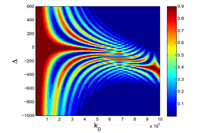
Figure 1: Contour plot of the fidelity between final states of the two cases.

3 The effect of kinetic energy term on QFI

Now let us turn back to the calculation of the QFI. For the $su$(2)-type Hamiltonian, a general solution for the QFI has been discussed [14]. We can define a Hermitian operator independent of the initial state

$$\mathcal{H}_{1}=\mathrm{i}(\partial_{\Omega}\hat{U}_{1}^{\dagger})\hat{U}_{1}.$$ (12)

If the initial state is pure state, the QFI can be expressed as

$$F=4\langle\psi_{in}|\Delta^{2}\mathcal{H}_{1}|\psi_{in}\rangle.$$ (13)

In fact, the momentum representation will facilitate our computation, as will see in A. We still use the initial state (10). After the evolution of the Hamiltonian (2), we finally get the integral formalism of QFI

$$F =4\Biggl{[}\frac{\sigma}{\hbar\sqrt{\pi}}\int_{-\infty}^{\infty}\mathrm{d}p\ \mathrm{e}^{-\frac{p^{2}\sigma^{2}}{\hbar^{2}}}\Biggl{\{}\left(\frac{\Omega^{2}\left(\sin\left(\omega t\right)-\omega t\right)}{2\omega^{3}}-\frac{\sin\left(\omega t\right)}{2\omega}\right)^{2}$$ (14)

$$+\left(\frac{\sqrt{\omega^{2}-\Omega^{2}}\left(1-\cos\left(\omega t\right)\right)}{2\omega^{2}}\right)^{2}+\left(\frac{\Omega\sqrt{\omega^{2}-\Omega^{2}}(\sin\left(\omega t\right)-\omega t)}{2\omega^{3}}\right)^{2}\Biggl{\}}\Biggl{]}$$

$$-4\Biggl{[}\frac{\sigma}{\hbar\sqrt{\pi}}\int_{-\infty}^{\infty}\mathrm{d}p\ \mathrm{e}^{-\frac{p^{2}\sigma^{2}}{\hbar^{2}}}\Biggl{(}\frac{\Omega\sqrt{\omega^{2}-\Omega^{2}}(\sin\left(\omega t\right)-\omega t)}{2\omega^{3}}\Biggr{)}\Biggr{]}^{2},$$

where

$$\omega=\sqrt{\left(\Delta+\frac{k_{0}\left(\frac{k_{0}\hbar}{2}+p\right)}{m}\right)^{2}+\Omega^{2}}.$$ (15)

Again, as for the case without the kinetic energy term, we can define a Hermitian operator independent of the initial state

$$\mathcal{H}_{2}=\mathrm{i}(\partial_{\Omega}\hat{U}_{2}^{\dagger})\hat{U}_{2}.$$ (16)

The whole procedure is similar to the above case, and we will continue to use the initial state $|\psi_{in}\rangle=|a\rangle|\psi_{0}\rangle$. Notably, when the kinetic energy term is absent, the calculation will be much easier, and we can get an analytical expression for the QFI written in A. After the evolution of the Hamiltonian (6), the QFI at $t$ will be:

$$F=\frac{\left(\Omega^{2}\omega^{\prime}t+\Delta^{2}\sin\left(\omega^{\prime}t\right)\right)^{2}+\Delta^{2}\omega^{\prime 2}\left(\cos\left(\omega^{\prime}t\right)-1\right)^{2}}{\omega^{\prime 6}},$$ (17)

where

$$\omega^{\prime}=\sqrt{\Delta^{2}+\Omega^{2}}.$$ (18)

We compare it with the QFI with kinetic energy term in figure 2 concerning the detuning and light’s momentum. Obviously, the QFI without the kinetic energy term does not dependent on $k_{0}$. When the kinetic energy term is taken into account, enhancing $k_{0}$ will lower the QFI drastically. We also conclude from the figures that if the detuning is positive at the given wave vector, the QFI without the kinetic energy term is always larger than that with the kinetic energy term, which means we will overestimate the precision of the Rabi frequency if we omit the kinetic energy. However, if the detuning is negative, the situation will become different and we will discuss it later. In addition, we can see that decreasing the absolute value of the detuning $\Delta$ will increase the QFI in both cases.

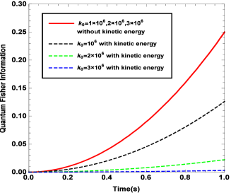
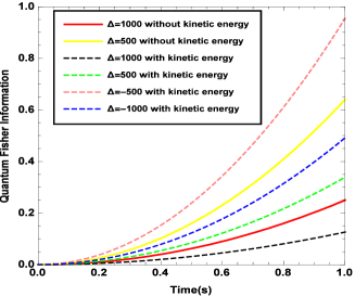
Figure 2: (a) QFI with (dashed line) or without (solid lines) kinetic energy using $k_{0}=10^{6},2\times 10^{6},2\times 10^{6}~{}\mathrm{m}^{-1}$ while setting $\Delta=1000\ \mathrm{s^{-1}}$. (b) QFI with (dashed lines) or without (solid lines) kinetic energy using $\Delta=1000,500,100~{}\mathrm{s}^{-1}$ while setting $\ k_{0}=10^{6}\ \mathrm{m^{-1}}$.

In order to see the influence of the detuning on the QFI more precisely, we plot the curve of QFI with respect to the detuning in figure 3. We can obtain the fact that the QFI without the kinetic energy term depends only on the absolute value of the detuning while that with the kinetic energy has an axis of symmetry slightly deviating from zero. That is the reason why the QFI without the kinetic energy term is larger when $\Delta>0$. When the detuning is negative and smaller than a specific value (about -200$\mathrm{s}^{-1}$) at the given $k_{0}$, the QFI without kinetic energy term is smaller than that with kinetic energy. It means we will underestimate the measurement precision if we neglect the kinetic energy term when detecting the Rabi frequency.

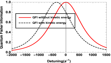
Figure 3: QFI with respect to $\Delta$, here we set $t=1\mathrm{s}$ and$\ k_{0}=10^{6}\ \mathrm{m^{-1}}$.

Nevertheless, unlike the case without the kinetic energy, in figure 4 we show how the Gaussian state’s variance $\sigma$ influences the QFI with the kinetic energy term.

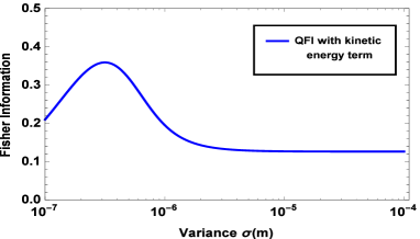
Figure 4: QFI with respect to $\sigma$, here we set $t=1\mathrm{s}$ ,$\ k_{0}=10^{6}\ \mathrm{m^{-1}}$, and $\Delta=10^{3}\ \mathrm{s^{-1}}$.

4 Practical measurement of Rabi frequency without kinetic energy

In general, we do not know if the QFI will be saturated in practical measurement. Although the QFI gives the theoretical best sensitivity, we still need to choose a particular measurement scheme to attain it. The CFI gives the sensitivity of a parameter (in our case $\Omega$), whose information is hidden in the probability distribution of an observable’s outcome. Therefore, we will find a realistic observable and examine the parameter sensitivity provided by measuring the given observable values. For simplicity, we will firstly check out the case without kinetic energy term in this section.

The definition of CFI in terms of a parameter $\theta$ is

$$I=\int P(\lambda|\theta)(\frac{\partial\ln P(\lambda|\theta)}{\partial\theta})^{2}\mathrm{d}\lambda,$$ (19)

where $P(\lambda|\theta)$ is the probability of obtaining $\lambda$ when we measure the observable $\hat{\Lambda}$ with the parameter being $\theta$. For example, if we carry out the population-difference measurement (PDM) $\hat{\Lambda}=\hat{S}_{z}$, then the CFI will be denoted as

$$I_{PDM}=\Sigma_{i=a,b}(\partial_{\Omega}P_{i})^{2}/P_{i}.$$ (20)

In the case of continuous variables, such as momentum measurement (MM) $\hat{\Lambda}=\hat{p}$, the analytical expression of the corresponding CFI is given below

$$I_{MM}=\int(\partial_{\Omega}P(p))^{2}/P(p)\mathrm{d}p.$$ (21)

To calculate the CFI with the $\hat{S}_{z}$, since we already know

$$I_{PDM}=\Sigma_{i=a,b}(\partial_{\Omega}P_{i})^{2}/P_{i}=(\partial_{\Omega}P_{a})^{2}/[P_{a}(1-P_{a})],$$ (22)

we can use $P_{a}=\langle\psi_{a}|\psi_{a}\rangle=|\langle a|\psi_{out}\rangle|^{2}$ to represent the probability of finding the final state in the internal state $|a\rangle$. Due to the result

$$|\psi_{a}\rangle =\langle a|\mathrm{e}^{-\mathrm{i}\frac{t}{\hbar}\hat{H}_{2}}|a\rangle|\psi_{0}\rangle=\langle a|W\mathrm{e}^{-\mathrm{i}\frac{t}{\hbar}\hat{H}_{e2}}W^{\dagger}|a\rangle|\psi_{0}\rangle$$ (23)

$$=\mathrm{e}^{-\mathrm{i}\frac{k_{0}\hat{z}}{2}}\langle a|\mathrm{e}^{-\mathrm{i}\frac{t}{\hbar}\hat{H}_{e2}}\mathrm{e}^{\mathrm{i}\frac{k_{0}\hat{z}}{2}}|a\rangle|\psi_{0}\rangle$$

$$=\langle a|\mathrm{e}^{-\mathrm{i}\frac{t}{\hbar}\hat{H}_{e2}}|a\rangle|\psi_{0}\rangle,$$

the probability is

$$P_{a}=|\langle a|\mathrm{e}^{-\mathrm{i}\frac{t}{\hbar}\hat{H}_{e2}}|a\rangle|^{2}=\cos^{2}c_{1}+n_{z1}^{2}\sin^{2}c_{1},$$ (24)

where

$$c_{1}=-\frac{t}{2}\omega^{\prime},n_{z1}=\frac{\Delta}{\omega^{\prime}}.$$ (25)

So we finally get our analytical solution of CFI:

$$I_{PDM}=\frac{2\left(2\Delta^{2}\omega^{\prime}\sin\left(\frac{1}{2}\omega^{\prime}t\right)+\omega^{\prime 2}t\Omega^{2}\cos\left(\frac{1}{2}\omega^{\prime}t\right)\right)^{2}}{\omega^{\prime 6}\left(2\Delta^{2}+\Omega^{2}\cos\left(\omega^{\prime}t\right)+\Omega^{2}\right)}.$$ (26)

In the following, we summarize the Fisher information (QFI, CFI for $\hat{S}_{z}$ ) in figure 5.

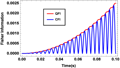
Figure 5: Fisher Information, in which the parameters are defaultly set as$\ k_{0}=10^{6}\ \mathrm{m^{-1}}$, and $\Delta=10^{3}\ \mathrm{s^{-1}}$.

We can see the Fisher information is so small that the final state almost does not contain information of $\Omega$. The situations become different when the parameters change, such as $\Delta$ for different values in figure 6.

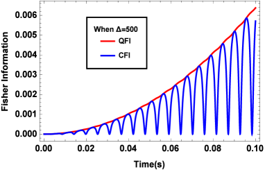
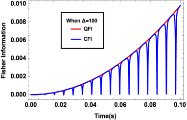
Figure 6: QFI and CFI when the kinetic energy term is absent for different detunings: $\Delta=500,100~{}\mathrm{s^{-1}}$ while keeping$\ k_{0}=10^{6}\ \mathrm{m^{-1}}$. We can see that the Fisher information basically become larger as the detuning decreases.

We obtain when the detuning becomes sufficiently small, the Fisher information becomes considerable. Fortunately, in the case where the kinetic energy term is omitted, the QFI will be saturated only through the population-difference measurement. Moreover, it appears that as the detuning goes down, the CFI matches QFI with higher probability. Actually, in the case of near resonance, the CFI of population-difference measurement coincides precisely with the results of QFI.

5 Practical measurement of Rabi frequency with kinetic energy

We will now turn to the case with the kinetic energy term to see if the QFI will be saturated. The same as the QFI, the CFI with the kinetic energy term is a little bit cumbersome. To calculate $I_{PDM}=(\partial_{\Omega}P_{a})^{2}/[P_{a}(1-P_{a})]$, we need to know $|\psi_{a}\rangle=\langle a|\psi_{out}\rangle$:

$$|\psi_{a}\rangle =\langle a|W\mathrm{e}^{-\mathrm{i}\frac{t}{\hbar}\hat{H}_{e1}}W^{\dagger}|a\rangle|\psi_{0}\rangle$$ (27)

$$=\langle a|\mathrm{e}^{-\mathrm{i}\frac{k_{0}}{2}\hat{z}}\mathrm{e}^{-\mathrm{i}\frac{t}{\hbar}\hat{H}_{e1}}\mathrm{e}^{\mathrm{i}\frac{k_{0}}{2}\hat{z}}|a\rangle|\psi_{0}\rangle$$

$$=\mathrm{e}^{-\mathrm{i}\frac{k_{0}}{2}\hat{z}}\mathrm{e}^{-\mathrm{i}\frac{t}{\hbar}(\frac{\hat{p}^{2}}{2m}+\frac{\hbar^{2}k_{0}^{2}}{8m}+\frac{\hbar\Delta}{2})}(\cos c_{2}-\mathrm{i}n_{z2}\sin c_{2})\mathrm{e}^{\mathrm{i}\frac{k_{0}}{2}\hat{z}}|\psi_{0}\rangle,$$

where the operators read

$$\hat{c}_{2}=-\frac{t}{\hbar}\sqrt{(\frac{\hbar\Omega}{2})^{2}+(\frac{\hbar k_{0}}{2m}\hat{p}+\frac{\hbar\Delta}{2})^{2}},$$ (28)

$$\hat{n}_{z2}=\frac{\frac{\hbar k_{0}}{2m}\hat{p}+\frac{\hbar\Delta}{2}}{\sqrt{(\frac{\hbar\Omega}{2})^{2}+(\frac{\hbar k_{0}}{2m}\hat{p}+\frac{\hbar\Delta}{2})^{2}}}.$$ (29)

As a result, we can get the probability:

$$P_{a} =\langle\psi_{0}|\mathrm{e}^{-\mathrm{i}\frac{k_{0}}{2}\hat{z}}(\cos^{2}c_{2}+n_{z2}^{2}\sin^{2}c_{2})\mathrm{e}^{\mathrm{i}\frac{k_{0}}{2}\hat{z}}|\psi_{0}\rangle$$ (30)

$$=\int\mathrm{d}p\langle\psi_{0}|\mathrm{e}^{-\mathrm{i}\frac{k_{0}}{2}\hat{z}}(\cos^{2}c_{2}+n_{z2}^{2}\sin^{2}c_{2})\mathrm{e}^{\mathrm{i}\frac{k_{0}}{2}\hat{z}}|p\rangle\langle p|\psi_{0}\rangle$$

$$=\int\mathrm{d}p|\langle\psi_{0}|p\rangle|^{2}(\cos^{2}c^{\prime}+n_{z}^{\prime 2}\sin^{2}c^{\prime}),$$

where

$$c^{\prime}=-\frac{t}{\hbar}\sqrt{(\frac{\hbar\Omega}{2})^{2}+(\frac{\hbar k_{0}}{2m}p+\frac{\hbar^{2}k_{0}^{2}}{4m}+\frac{\hbar\Delta}{2})^{2}},$$ (31)

$$n_{z}^{\prime}=\frac{\frac{\hbar k_{0}}{2m}p+\frac{\hbar^{2}k_{0}^{2}}{4m}+\frac{\hbar\Delta}{2}}{\sqrt{(\frac{\hbar\Omega}{2})^{2}+(\frac{\hbar k_{0}}{2m}p+\frac{\hbar^{2}k_{0}^{2}}{4m}+\frac{\hbar\Delta}{2})^{2}}}.$$ (32)

Then we can get the integral formalism of CFI for population-difference measurement. Nevertheless, in this case, the CFI is extremely small compared to the QFI, which means the population-difference measurement is not a good candidate for estimating $\Omega$. However, since the QFI, as the maximum of CFI, is large, we can believe some measurement should facilitate the ascent of CFI. If we carry out a combined measurement (CM) that resolves the internal states and the momentum distribution $\hat{\Lambda}=(\hat{S}_{z},\hat{p})$, the CFI is

$$I_{CM}=\sum_{s=a,b}\int\mathrm{d}p\frac{[\partial_{\Omega}P_{s}(p)]^{2}}{P_{s}(p)},$$ (33)

where

$$P_{s}(p)=|\langle\psi_{0}|p\rangle|^{2}(\cos^{2}c^{\prime}+n_{z}^{\prime 2}\sin^{2}c^{\prime}).$$ (34)

As a result of this kind of measurement, we continue to maintain $\ k_{0}=10^{6}\ \mathrm{m^{-1}}$, $\Delta=10^{3}\ \mathrm{s^{-1}}$, and we show the CFI becomes larger in figure 7, meaning we will gain more information about the parameter.

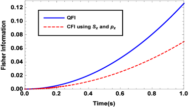
Figure 7: Fisher Information with kinetic energy while measuring $S_{z}$ and $p_{z}$.

Notably, this is the region where the kinetic energy term cannot be neglected, so it is just an illusion that using population-difference measurement alone can saturate the maximal QFI according to the last section. As a result, when we take the kinetic energy into account, we need to choose different measurement schemes to reach or just approach the maximal QFI. Our result indicates that the neglect of the kinetic energy term will make people carry out incorrect measurements, which they thought has attained the maximal measuring accuracy of Rabi frequency, whereas they are not in some regimes.

6 Conclusion

In summary, we have theoretically investigated the effect of kinetic energy on the measuring precision of the Rabi frequency. Through transforming the original Hamiltonian into a $su$(2)-type Hamiltonian, we can obtain the analytical expressions of the QFI and CFI indicating the frequency uncertainty.

We now list our main results in the following. Firstly, only when the absolute value of the detuning or the wave vector is small enough can we safely omit the kinetic energy term, which we can conclude from both the fidelity and the QFI. Meanwhile, reducing the two parameters can enhance the QFI in cases with or without the kinetic energy in Hamiltonian. Secondly, the inappropriate omission of the kinetic energy term will lead to overestimating the measuring accuracy of Rabi frequency when $\Delta>0$ or inducing underestimating the precision when $\Delta$ is smaller than some negative value at the given wave vector. Thirdly, a particular initial state’s variance in position space can attain a maximum in QFI while taking the kinetic energy term into account. Lastly, although we found that the population-difference measurement is not adequate for CFI with the kinetic energy term, inclusion of the momentum measurement will help a lot.

The Fisher information in different regions of parameters can be deduced from our expressions, and they can contribute to the precise measurement of the Rabi frequency in realistic situations. For example, to improve the measuring accuracy, experimentalists can use our method to calculate the QFI in their interested regime and determine whether the kinetic energy term can be safely omitted. If the parameters do not satisfy the valid neglect, observers need to take care of the schemes of measurement since they may not optimize the precision. Our result may exhibit its value especially in cold atom and atom interferometry [2, 42].

Appendix A Detailed calculation of the quantum Fisher information

We use the crucial result of the article [14]. For the $su$(2)-type Hamiltonian $\hat{H}=\vec{r}(\phi)\cdot\vec{J}$, we focus on a unitary parametrization $\hat{U}=\mathrm{e}^{-\mathrm{i}\hat{H}(\phi)t}$ (here we set $\hbar=1$ and we can recover it after the whole calculation using dimension analysis). Then we can define a Hermitian operator $\mathcal{H}=\mathrm{i}(\partial_{\phi}\hat{U}^{\dagger})\hat{U}$ and a velocity vector $\vec{v}=\frac{\mathrm{d}\vec{r}}{\mathrm{d}\theta}$. For an initial pure state $|\psi\rangle$, we have the QFI for the final state: $F=4(\langle\mathcal{H}^{2}\rangle-\langle\mathcal{H}\rangle^{2})$, where the

$$\mathcal{H} = \frac{(\vec{r}\cdot\vec{v})(\sin(|\vec{r}|t)-|\vec{r}|t)}{|\vec{r}|^{3}}\vec{r}\cdot\vec{J}-\frac{\sin(|\vec{r}|t)}{|\vec{r}|}\vec{v}\cdot\vec{J}$$ (35)

$$+\frac{1-\cos(|\vec{r}|t)}{|\vec{r}|^{2}}(\vec{r}\times\vec{v})\cdot\vec{J}$$

$$= \vec{R}\cdot\vec{\sigma}.$$

Case 1: the QFI with the kinetic energy

$$\mathcal{\mathcal{H}}_{1} =\mathrm{i}(\partial_{\Omega}\hat{U}_{1}^{\dagger})\hat{U}_{1}=\mathrm{i}\hat{W}(\partial_{\Omega}\mathrm{e}^{\mathrm{i}t\hat{H}_{e1}})\mathrm{e}^{-\mathrm{i}t\hat{H}_{e1}}\hat{W}^{\dagger}$$ (36)

$$=\mathrm{i}\hat{W}(\partial_{\Omega}\mathrm{e}^{\mathrm{i}t(\vec{r}\cdot\vec{J})})\mathrm{e}^{-\mathrm{i}t(\vec{r}\cdot\vec{J})}\hat{W}^{\dagger}$$

$$=\hat{W}\mathcal{H}^{{}^{\prime}}\hat{W}^{\dagger},$$

where $\vec{r}=(\Omega,0,\frac{k_{0}}{m}\hat{p}+\Delta)$, $\vec{v}=(1,0,0)$.

So $\mathcal{H}^{{}^{\prime}}=\vec{R}\cdot\vec{\sigma}$,

$$\vec{R}= \biggl{(}\frac{\Omega^{2}(\sin(|\vec{r}|t)-|\vec{r}|t)}{2|\vec{r}|^{3}}-\frac{\sin(|\vec{r}|t)}{2|\vec{r}|},$$ (37)

$$\frac{1-\cos(|\vec{r}|t)}{2|\vec{r}|^{2}}(\frac{k_{0}}{m}\hat{p}+\Delta),\frac{\Omega(\sin(|\vec{r}|t)-|\vec{r}|t)}{2|\vec{r}|^{3}}(\frac{k_{0}}{m}\hat{p}+\Delta)\biggr{)}.$$

We use the following initial state:

$$\langle p|\psi_{0}\rangle =\int_{-\infty}^{\infty}\langle p|z\rangle\langle z|\psi_{0}\rangle=\frac{\sqrt{\sigma}}{\sqrt[4]{\pi}}\mathrm{e}^{-\frac{p^{2}\sigma^{2}}{2\hbar^{2}}}.$$ (38)

Then,

$$\hat{W}^{\dagger}|a,\psi_{0}\rangle =\int_{-\infty}^{\infty}\mathrm{e}^{\mathrm{i}\frac{k_{0}\hat{z}}{2}}|p\rangle\mathrm{d}p\langle p|\psi_{0}\rangle|a\rangle$$ (39)

$$=\int_{-\infty}^{\infty}\mathrm{d}p\frac{\sqrt{\sigma}}{\sqrt[4]{\pi}}\mathrm{e}^{-\frac{p^{2}\sigma^{2}}{2\hbar^{2}}}\mathrm{e}^{\mathrm{i}\frac{k_{0}\hat{z}}{2}}|p\rangle|a\rangle,$$

we can simplify the above as

$$\hat{W}^{\dagger}|a,\psi_{0}\rangle =\int_{-\infty}^{\infty}\mathrm{d}p\frac{\sqrt{\sigma}}{\sqrt[4]{\pi}}\mathrm{e}^{-\frac{p^{2}\sigma^{2}}{2\hbar^{2}}}|p+\frac{\hbar k_{0}}{2}\rangle|a\rangle.$$ (40)

Finally we obtain

$$\langle\mathcal{\mathcal{H}}_{1}\rangle =-\frac{\sigma}{\sqrt{\pi}}\int_{-\infty}^{\infty}\mathrm{d}p\mathrm{e}^{-\frac{p^{2}\sigma^{2}}{\hbar^{2}}}\langle p+\frac{\hbar k_{0}}{2}|\hat{R}_{z}|p+\frac{\hbar k_{0}}{2}\rangle,$$ (41)

and

$$\langle\mathcal{H}_{1}^{2}\rangle =\frac{\sigma}{\sqrt{\pi}}\int_{-\infty}^{\infty}\mathrm{d}p\mathrm{e}^{-\frac{p^{2}\sigma^{2}}{\hbar^{2}}}\langle p+\frac{\hbar k_{0}}{2}|\hat{R}^{2}|p+\frac{\hbar k_{0}}{2}\rangle.$$ (42)

$$F= 4\Biggl{[}\frac{\sigma}{\hbar\sqrt{\pi}}\int_{-\infty}^{\infty}\mathrm{d}p\ \mathrm{e}^{-\frac{p^{2}\sigma^{2}}{\hbar^{2}}}\Biggl{\{}\left(\frac{\Omega^{2}\left(\sin\left(\omega t\right)-\omega t\right)}{2\omega^{3}}-\frac{\sin\left(\omega t\right)}{2\omega}\right)^{2}$$ (43)

$$+\left(\frac{\sqrt{\omega^{2}-\Omega^{2}}\left(1-\cos\left(\omega t\right)\right)}{2\omega^{2}}\right)^{2}+\left(\frac{\Omega\sqrt{\omega^{2}-\Omega^{2}}(\sin\left(\omega t\right)-\omega t)}{2\omega^{3}}\right)^{2}\Biggl{\}}\Biggl{]}$$

$$-4\Biggl{[}\frac{\sigma}{\hbar\sqrt{\pi}}\int_{-\infty}^{\infty}\mathrm{d}p\ \mathrm{e}^{-\frac{p^{2}\sigma^{2}}{\hbar^{2}}}\Biggl{(}\frac{\Omega\sqrt{\omega^{2}-\Omega^{2}}(\sin\left(\omega t\right)-\omega t)}{2\omega^{3}}\Biggr{)}\Biggr{]}^{2}.$$

where

$$\omega=\sqrt{\left(\Delta+\frac{k_{0}\left(\frac{k_{0}\hbar}{2}+p\right)}{m}\right)^{2}+\Omega^{2}}.$$ (44)

Case 2: the QFI without the kinetic energy

$$\mathcal{H}_{2} =\mathrm{i}(\partial_{\Omega}\hat{U}_{2}^{\dagger})U_{2}=\mathrm{i}\hat{W}(\partial_{\Omega}\mathrm{e}^{\mathrm{i}t\hat{H}_{e2}})\mathrm{e}^{-\mathrm{i}t\hat{H}_{e2}}\hat{W}^{\dagger}$$ (45)

$$=\mathrm{i}\hat{W}(\partial_{\Omega}\mathrm{e}^{\mathrm{i}t(\vec{r}\cdot\vec{J})})\mathrm{e}^{-\mathrm{i}t(\vec{r}\cdot\vec{J})}\hat{W}^{\dagger}$$

$$=\hat{W}\mathcal{H}^{{}^{\prime}}\hat{W}^{\dagger},$$

where $\vec{J}=\frac{\vec{\sigma}}{2}$, $\vec{r}=(\Omega,0,\Delta)$, $\vec{v}=\frac{\mathrm{d}\vec{r}}{\mathrm{d}\Omega}=(1,0,0)$.

$$\mathcal{H}^{{}^{\prime}} = \frac{\Omega(\sin(|\vec{r}|t)-|\vec{r}|t)}{|\vec{r}|^{3}}(\frac{\Omega}{2}\sigma_{x}+\frac{\Delta}{2}\sigma_{z})$$ (46)

$$-\frac{\sin(|\vec{r}|t)}{|\vec{r}|}\frac{\sigma_{x}}{2}+\frac{1-\cos(|\vec{r}|t)}{|\vec{r}|^{2}}\frac{\Delta}{2}\sigma_{y}$$

$$= \vec{R}\cdot\vec{\sigma},$$

where

$$\vec{R}= \biggl{(}\frac{\Omega^{2}(\sin(|\vec{r}|t)-|\vec{r}|t)}{2|\vec{r}|^{3}}-\frac{\sin(|\vec{r}|t)}{2|\vec{r}|},$$ (47)

$$\frac{1-\cos(|\vec{r}|t)}{2|\vec{r}|^{2}}\Delta,\frac{\Omega(\sin(|\vec{r}|t)-|\vec{r}|t)}{2|\vec{r}|^{3}}\Delta\biggr{)}.$$

Since the Fisher Information $F=4(\langle\mathcal{H}_{2}^{2}\mathcal{\rangle}-\langle\mathcal{H}_{2}\rangle^{2})$, the initial state is $|a,\psi_{0}\rangle$, where $\langle z|\psi_{0}\rangle=\frac{1}{\sqrt[4]{\pi\sigma^{2}}}\exp(-\frac{z^{2}}{2\sigma^{2}})$. Then due to $\hat{W}^{\dagger}|a,\psi_{0}\rangle=|a\rangle\mathrm{e}^{\mathrm{i}\frac{k_{0}\hat{z}}{2}}|\psi_{0}\rangle$, the z-space doesn’t contribute to the final Fisher information.

$$F=\frac{\left(\Omega^{2}\omega^{\prime}t+\Delta^{2}\sin\left(\omega^{\prime}t\right)\right)^{2}+\Delta^{2}\omega^{\prime 2}\left(\cos\left(\omega^{\prime}t\right)-1\right)^{2}}{\omega^{\prime 6}},$$ (48)

where

$$\omega^{\prime}=\sqrt{\Delta^{2}+\Omega^{2}}.$$ (49)

Appendix B Detailed Derivation of the fidelity

In this appendix, we show how the fidelity (11) is calculated in detail.

$$\mathcal{F} =|\langle\psi_{0}|\langle a|\hat{W}\mathrm{e}^{\mathrm{i}\frac{t}{\hbar}\hat{H}_{e1}}\mathrm{e}^{-\mathrm{i}\frac{t}{\hbar}\hat{H}_{e2}}\hat{W}^{\dagger}|a\rangle|\psi_{0}\rangle|^{2}$$ (50)

$$=|\langle\psi_{0}|\langle a|\mathrm{e}^{-\mathrm{i}\frac{k_{0}\hat{z}}{2}}\mathrm{e}^{\mathrm{i}\frac{t}{\hbar}\hat{H}_{e1}}\mathrm{e}^{-\mathrm{i}\frac{t}{\hbar}\hat{H}_{e2}}\mathrm{e}^{\mathrm{i}\frac{k_{0}\hat{z}}{2}}|a\rangle|\psi_{0}\rangle|^{2}$$

$$=|\langle\psi_{0}|\mathrm{e}^{-\mathrm{i}\frac{k_{0}\hat{z}}{2}}\mathrm{e}^{\mathrm{i}\frac{t}{\hbar}(\frac{\hat{p}^{2}}{2m}+\frac{\hbar^{2}k_{0}^{2}}{8m})}\langle a|\mathrm{e}^{\mathrm{i}\frac{t}{\hbar}[\frac{\hbar\Omega}{2}\sigma_{x}+(\frac{\hbar k_{0}\hat{p}}{2m}+\frac{\hbar\Delta}{2})\sigma_{z}]}\mathrm{e}^{-\mathrm{i}\frac{t}{\hbar}[\frac{\hbar\Omega}{2}\sigma_{x}+\frac{\hbar\Delta}{2}\sigma_{z}]}|a\rangle\mathrm{e}^{\mathrm{i}\frac{k_{0}\hat{z}}{2}}|\psi_{0}\rangle|^{2}$$

We set $c=\frac{t}{\hbar}\sqrt{(\frac{\hbar k_{0}\hat{p}}{2m}+\frac{\hbar\Delta}{2})^{2}+(\frac{\hbar\Omega}{2})^{2}}$, $\vec{m}=(\frac{\frac{\hbar\Omega}{2}}{\sqrt{(\frac{\hbar k_{0}\hat{p}}{2m}+\frac{\hbar\Delta}{2})^{2}+(\frac{\hbar\Omega}{2})^{2}}},0,\frac{\frac{\hbar k_{0}\hat{p}}{2m}+\frac{\hbar\Delta}{2}}{\sqrt{(\frac{\hbar k_{0}\hat{p}}{2m}+\frac{\hbar\Delta}{2})^{2}+(\frac{\hbar\Omega}{2})^{2}}})$, and using the exponential expand of the pauli matrix, we can get the expression:

$$\mathrm{e}^{\mathrm{i}\frac{t}{\hbar}[\frac{\hbar\Omega}{2}\sigma_{x}+(\frac{\hbar k_{0}\hat{p}}{2m}+\frac{\hbar\Delta}{2})\sigma_{z}]}=\cos c+\mathrm{i}(m_{1}\sigma_{x}+m_{3}\sigma_{z})\sin c.$$ (51)

Similarly, we set $d=-\frac{t}{\hbar}\sqrt{(\frac{\hbar\Delta}{2})^{2}+(\frac{\hbar\Omega}{2})^{2}}$, $\vec{n}=(\frac{\frac{\hbar\Omega}{2}}{\sqrt{(\frac{\hbar\Delta}{2})^{2}+(\frac{\hbar\Omega}{2})^{2}}},0,\frac{\frac{\hbar\Delta}{2}}{\sqrt{(\frac{\hbar\Delta}{2})^{2}+(\frac{\hbar\Omega}{2})^{2}}})$ and substitute these into the other complex exponential expand:

$$\mathrm{e}^{-\mathrm{i}\frac{t}{\hbar}[\frac{\hbar\Omega}{2}\sigma_{x}+\frac{\hbar\Delta}{2}\sigma_{z}]}=\cos d+\mathrm{i}(n_{1}\sigma_{x}+n_{3}\sigma_{z})\sin d.$$ (52)

Then the inner product of the internal states can be calculated as

$$\langle a|\mathrm{e}^{\mathrm{i}\frac{t}{\hbar}[\frac{\hbar\Omega}{2}\sigma_{x}+(\frac{\hbar k_{0}\hat{p}}{2m}+\frac{\hbar\Delta}{2})\sigma_{z}]}\mathrm{e}^{-\mathrm{i}\frac{t}{\hbar}[\frac{\hbar\Omega}{2}\sigma_{x}+\frac{\hbar\Delta}{2}\sigma_{z}]}|a\rangle$$

$$= \langle a|[\cos c+\mathrm{i}(m_{1}\sigma_{x}+m_{3}\sigma_{z})\sin c]|a\rangle\langle a|[\cos d+\mathrm{i}(n_{1}\sigma_{x}+n_{3}\sigma_{z})\sin d]|a\rangle$$

$$+\langle a|[\cos c+\mathrm{i}(m_{1}\sigma_{x}+m_{3}\sigma_{z})\sin c]|b\rangle\langle b|[\cos d+\mathrm{i}(n_{1}\sigma_{x}+n_{3}\sigma_{z})\sin d]|a\rangle$$

$$= (\cos c-\mathrm{i}m_{3}\sin c)(\cos d-\mathrm{i}n_{3}\sin d)+\mathrm{i}m_{1}\sin c\ \mathrm{i}n_{1}\sin d$$

$$= \cos c\cos d-\mathrm{i}m_{3}\sin c\cos d-\mathrm{i}n_{3}\sin d\cos c$$

$$-m_{3}\sin c\ n_{3}\sin d-m_{1}\sin c\ n_{1}\sin d$$

$$= \cos c\cos d-\mathrm{i}m_{3}\sin c\cos d$$ (53)

$$-\mathrm{i}n_{3}\sin d\cos c-(m_{3}n_{3}+m_{1}n_{1})\sin c\sin d.$$

Now we see that the overlap between the two evolved final state is

$$\langle\psi_{0}|\mathrm{e}^{-\mathrm{i}\frac{k_{0}\hat{z}}{2}}\mathrm{e}^{\mathrm{i}\frac{t}{\hbar}(\frac{\hat{p}^{2}}{2m}+\frac{\hbar^{2}k_{0}^{2}}{8m})}\langle a|\mathrm{e}^{\mathrm{i}\frac{t}{\hbar}[\frac{\hbar\Omega}{2}\sigma_{x}+(\frac{\hbar k_{0}\hat{p}}{2m}+\frac{\hbar\Delta}{2})\sigma_{z}]}\mathrm{e}^{-\mathrm{i}\frac{t}{\hbar}[\frac{\hbar\Omega}{2}\sigma_{x}+\frac{\hbar\Delta}{2}\sigma_{z}]}|a\rangle\mathrm{e}^{\mathrm{i}\frac{k_{0}\hat{z}}{2}}|\psi_{0}\rangle$$

$$= \int\mathrm{d}p|\langle\psi_{0}|p\rangle|^{2}[\mathrm{e}^{\mathrm{i}\frac{t}{\hbar}(\frac{\hat{p}^{2}}{2m}+\frac{\hbar^{2}k_{0}^{2}}{8m})}(\cos c\cos d-\mathrm{i}m_{3}\sin c\cos d$$ (54)

$$-\mathrm{i}n_{3}\sin d\cos c-(m_{3}n_{3}+m_{1}n_{1})\sin c\sin d)],$$

where $\hat{p}$ is replaced by $p+\frac{\hbar k_{0}}{2}$ ($c$ also includes $\hat{p}$). Then the modulus square, fidelity $\mathcal{F}$, can be numerically integrated.

References

References

[1] Louisell W H 1973 Quantum statistical properties of radiation (Wiley New York).
[2] Meystre P 2001 Atom optics (Springer Science & Business Media).
[3] Lukin M D 2003 Rev. Mod. Phys.75 457.
[4] Leibfried D, Blatt R, Monroe C, and Wineland D 2003 Rev. Mod. Phys.75 281.
[5] Robins N, Altin P, Debs J, and Close J 2013 Phys. Rep.529, 265-296.
[6] Müller H, Chiow S W, Long Q, Herrmann S, and Chu S 2008 Phys. Rev. Lett.100 180405.
[7] Mazzoni T, Zhang X, Del Aguila R, Salvi L, Poli N, and Tino G M 2015 Phys. Rev. A92 053619.
[8] Holevo A S 2011 Probabilistic and statistical aspects of quantum theory (Springer Science & Business Media).
[9] Helstrom C W 1976 Quantum detection and estimation theory (Academic press).
[10] Braunstein S L and Caves C M 1994 Phys. Rev. Lett.72 3439.
[11] Demkowicz-Dobrzański R, Jarzyna M and Kołodyński J 2015 Prog. Opt. vol 60 (Elsevier) pp 345-435.
[12] Dorner U 2012 New J. Phys.14 043011.
[13] Liu J, Yuan H-D, Lu X-M and Wang X-G 2019 J. Phys. A: Math. Theor.53 023001.
[14] Jing X-X, Liu J, Xiong H-N and Wang X-G 2015 Phys. Rev. A92 012312.
[15] Liu J, Jing X-X and Wang X-G 2015 Sci. Rep.5 8565.
[16] Pang S S and Brun T A 2014 Phys. Rev. A90 022117.
[17] Pezzé L, Li Y, Li W and Smerzi A 2016 Proc. Natl. Acad. Sci. U. S. A.113 11459.
[18] Chalopin T, Bouazza C, Evrard A, Makhalov V, Dreon D, Dalibard J, Sidorenkov L A and Nascimbene S 2018 Nat. Commun.9 4955.
[19] Degen C L, Reinhard F and Cappellaro P 2017 Rev. Mod. Phys.89 035002.
[20] Pezzé L, Smerzi A, Oberthaler M K, Schmied R and Treutlein R 2018 Rev. Mod. Phys.90 035005
[21] Gentile T R, Hughey B J, Kleppner D, and Ducas T W 1989 Phys. Rev. A40 5103.
[22] Knight P L and Milonni P W 1980 Phys. Rep.66 21-107.
[23] Kiilerich A H and Mølmer K 2014 Phys. Rev. A89 052110.
[24] Gammelmark S and Mølmer K 2014 Phys. Rev. Lett.112 170401.
[25] Metwally N and Hassan S S 2017 Laser Phys. Lett., 14 115204.
[26] Zhang J-H, Um M, Lv D, Zhang J-N, Duan L-M and Kim K 2018 Phys. Rev. Lett.121 160502.
[27] Tonekaboni B, Haine S A and Szigeti S S 2015 Phys. Rev. A91 033616.
[28] Li S-S 2011 Int. J. Theor. Phys.50 767.
[29] Yi X-X 1996 Commun. Theor. Phys.26 249.
[30] Kasevich M and Chu S 1992 Appl. Phys. B54 321.
[31] Edwards M, Griggs D A, Holman P L, Clark C W, Rolston S L and Phillips W D 1999 J. Phys. B32 2935.
[32] Hagley E W, Deng L, Kozuma M, Wen J, Helmerson K, Rolston S L and Phillips W D 1999 Science283 1706.
[33] Haine S A and Hope J J 2005 Phys. Rev. A72 033601.
[34] Wang X-G and Sun C-P 1995 J. Mod. Opt.42 515.
[35] Reetz-Lamour M, Deiglmayr J, Amthor T and Weidemüller M 2008 New J. Phys.10 045026.
[36] Law C K 2013 Phys. Rev. A87 045804.
[37] Sun C-P, Yi X-X, Zhao S-R, Zhang L and Wang C 1997 Quantum Semiclassic. Opt.9 119.
[38] Kritsotakis M, Szigeti S S, Dunningham J A and Haine S A 2018 Phys. Rev. A98 023629.
[39] Robins N P, Figl C, Haine S A, Morrison A K, Jeppesen M, Hope J J and Close J D 2006 Phys. Rev. Lett.96, 140403.
[40] Johnsson M T and Haine S A 2007 Phys. Rev. Lett.99 010401.
[41] Matthews M R, Anderson B P, Haljan P C, Hall D S, Holland M J, Williams J E, Wieman C E and Cornell E A 1999 Phys. Rev. Lett.83 3358.
[42] Cronin A D, Schmiedmayer J and Pritchard D E 2009 Rev. Mod. Phys.81 1051.