Microlocal analysis and characterization of Sobolev wavefront sets using shearlets

Abstract.

Sobolev wavefront sets and $2$-microlocal spaces play a key role in describing and analyzing the singularities of distributions in microlocal analysis and solutions of partial differential equations. Employing the continuous shearlet transform to Sobolev spaces, in this paper we characterize the microlocal Sobolev wavefront sets, the $2$-microlocal spaces, and local Hölder spaces of distributions/functions. We then establish the connections among Sobolev wavefront sets, $2$-microlocal spaces, and local Hölder spaces through the continuous shearlet transform.

1. Introduction and main results

The continuous wavelet transform (CWT) has many applications such as signal and image processing for providing time-scale analysis of various types of data and functions. Recall that the continuous wavelet transform of a function $f\in L^{2}(\mathbb{R})$ is defined to be

(1.1) $$\tilde{f}(a,b):=\int_{\mathbb{R}}|a|^{-\frac{1}{2}}\overline{\psi\left(\tfrac{x-b}{a}\right)}f(x)dx,\qquad a\in\mathbb{R}\backslash\{0\},b\in\mathbb{R},$$

where $\psi\in L^{2}(\mathbb{R})$ is an admissible wavelet satisfying $C_{\psi}:=\int_{\mathbb{R}}\frac{|\widehat{\psi}(\xi)|^{2}}{|\xi|}d\xi<\infty$. Here $\widehat{f}(\xi):=\int_{\mathbb{R}}f(x)e^{-2\pi ix\xi}dx$ for $\xi\in\mathbb{R}$ is the Fourier transform of $f\in L^{1}(\mathbb{R})$ and is extended to tempered distributions. The function $f$ can be recovered from its CWT through

$$f(x)=\frac{1}{C_{\psi}}\int_{\mathbb{R}}\int_{\mathbb{R}}\tilde{f}(a,b)\psi\left(\tfrac{x-b}{a}\right)\frac{dadb}{a^{2}},$$

with convergence of the integral in the weak sense. Discretizing the continuous wavelet transform by restricting $(a,b)$ in (1.1) to a discrete subset of $\mathbb{R}^{2}$, the (discretized) wavelets and their associated discrete wavelet expansions are often used to effectively and sparsely represent functions having point-like discontinuity/singularity, thanks to the good time-frequency localization and high vanishing moments of the underlying wavelet function $\psi$. In multiple dimensions, singularities of discontinuity across a curve such as edges in an image often hold the key information of a multidimensional function/signal or the solution of a partial differential equation. Though discrete wavelet expansions using classical wavelets are known to be optimal for capturing point-like singularities, using isotropic dilations of wavelet functions, they are not that effective for capturing curve-like singularities. Motivated by the ineffectiveness of wavelets for curve-like singularities, curvelets using rotation in Candés and Donoho [3] and shearlets using shear transform in [6], whose underlying systems are discrete affine systems, provide an optimally sparse approximation of a cartoon-type image with discontinuity/singularity across a $C^{2}$ smooth curve.

For a nonempty open subset $\Omega\subseteq\mathbb{R}^{d}$, the test function space $\mathcal{D}(\Omega)$ consists of all compactly supported $C^{\infty}$ functions $\varphi:\Omega\rightarrow\mathbb{C}$ such that $\operatorname{supp}(\varphi)\subseteq\Omega$. Then its dual space $\mathcal{D}^{\prime}(\Omega)$ consists of all distributions in $\Omega$. Our main goal of this paper is to characterize the Sobolev wavefront set of a distribution $f\in\mathcal{D}^{\prime}(\Omega)$ and the $2$-microlocal space of a function using the continuous shearlet transform for Sobolev spaces, and then to explore their connections with local Hölder regularity. Before presenting the main results of this paper, we first briefly review the continuous shearlet transform and Sobolev wavefront sets of a distribution.

1.1. Continuous shearlet transform

Shearlets are related to wavelets with composite dilations, which were introduced in [7]. Using shear transform to preserve the rectangular grid/lattice structure, shearlets have been introduced in [6, 20]. Let the (horizontal) shearlet $\psi\in L^{2}(\mathbb{R}^{2})$ be given by

(1.2) $$\widehat{\psi}(\xi)=\widehat{\psi}(\xi_{1},\xi_{2}):=\widehat{\psi_{1}}(\xi_{1})\widehat{\psi_{2}}\left({\xi_{2}}/{\xi_{1}}\right),\qquad\mbox{for}\;\xi=(\xi_{1},\xi_{2})\in\mathbb{R}^{2},\ \xi_{1}\neq 0,$$

where the one-dimensional functions $\psi_{1}$ and $\psi_{2}$ satisfy the following conditions:

• The function $\psi_{1}\in L^{2}(\mathbb{R})$ satisfies the Calderón condition $\int_{0}^{\infty}|\widehat{\psi_{1}}(a)|^{2}\frac{da}{a}=\int_{0}^{\infty}|\widehat{\psi_{1}}(-a)|^{2}\frac{da}{a}=1$, which is equivalent to

  (1.3) $$\int_{0}^{\infty}|\widehat{\psi_{1}}(a\xi)|^{2}\frac{da}{a}=1,\qquad\mbox{for all}\ \xi\in\mathbb{R}\backslash\{0\}$$

  and $\widehat{\psi_{1}}\in\mathcal{D}(\mathbb{R})$ with $\operatorname{supp}(\widehat{\psi_{1}})\subseteq[-2,-\frac{1}{2}]\cup[\frac{1}{2},2].$

• $\|\widehat{\psi_{2}}\|_{L^{2}}=1$ and $\widehat{\psi_{2}}\in\mathcal{D}(\mathbb{R})$ with $\operatorname{supp}(\widehat{\psi_{2}})\subseteq[-1,1]$.

If a shearlet $\psi$ is defined through (1.2), then throughout the paper we always assume that $\psi_{1}$ and $\psi_{2}$ satisfy the conditions in (C1) and (C2). Define the shear matrix $S_{s}$, the parabolic scaling matrix $D_{a}$ and the matrix $M_{as}$ by

(1.4) $$S_{s}:=\begin{bmatrix}1&-s\\ 0&1\end{bmatrix},\qquad D_{a}:=\begin{bmatrix}a&0\\ 0&\sqrt{a}\end{bmatrix},\qquad M_{as}:=S_{s}D_{a}=\begin{bmatrix}a&-\sqrt{a}s\\ 0&\sqrt{a}\end{bmatrix}.$$

We shall use the following notation for shearlet elements:

(1.5) $$\psi_{ast}:=a^{-{3}/{4}}\psi\left(M_{as}^{-1}(\cdot-t)\right)=a^{-{3}/{4}}\psi\left(D_{a}^{-1}S_{s}^{-1}(\cdot-t)\right).$$

Then $\{\psi_{ast}\;:\;a\in(0,1],\ s\in[-2,2],t\in\mathbb{R}^{2}\}$ is called a (horizontal) continuous shearlet system for $L^{2}(\mathcal{C})^{\vee}:=\{f\in L^{2}(\mathbb{R})\;:\;\operatorname{supp}(\widehat{f})\subseteq\mathcal{C}\}$, where $\mathcal{C}$ is the horizontal cone given by

(1.6) $$\mathcal{C}:=\left\{(\xi_{1},\xi_{2})\in\mathbb{R}^{2}\;:\;|\xi_{1}|\geq 2\quad\mbox{and}\quad|{\xi_{2}}/{\xi_{1}}|\leq 1\right\}.$$

The vertical continuous shearlet system is obtained by switching the role of the horizontal and vertical axes. More precisely, the (vertical) shearlet $\psi^{(v)}:=\psi(J\cdot)$ and

$$\psi^{(v)}_{ast}:=a^{-3/4}\psi^{(v)}(JM_{as}^{-1}J(\cdot-t))=a^{-3/4}\psi(M_{as}^{-1}J(\cdot-t))=\psi_{as(Jt)}(J\cdot),$$

where $J:\mathbb{R}^{2}\rightarrow\mathbb{R}^{2}$ is the matrix mapping $(x,y)$ to $(y,x)$. The (horizontal) continuous shearlet transform (CST) and the (vertical) CST of a function $f$ on $\mathbb{R}^{2}$ is defined by

$$\mathcal{SH}_{\psi}f(a,s,t):=\left\langle f,\psi_{ast}\right\rangle,\qquad\mathcal{SH}^{(v)}_{\psi}f(a,s,t):=\langle f,\psi^{(v)}_{ast}\rangle,$$

for $a\in(0,1]$, $s\in[-2,2]$, and $t\in\mathbb{R}^{2}$. Note that $\mathcal{SH}^{(v)}_{\psi}f(a,s,t)=\mathcal{SH}_{\psi}(f(J\cdot))(a,s,Jt)$. Due to the conditions in (C1) and (C2) on $\psi_{1}$ and $\psi_{2}$, the horizontal and vertical shearlets are bandlimited. See Figure 1.1 for the frequency support of the shearlets for different values of $a$ and $s$.

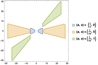
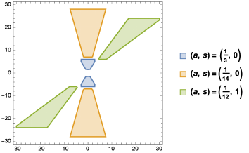
Figure 1.1. The left-hand side is the support of $\widehat{\psi_{ast}}$ for horizontal shearlet elements. Note that $|\widehat{\psi_{ast}}|=|\widehat{\psi_{as0}}|$. The right-hand side is the support of $\widehat{\psi^{(v)}_{ast}}$ for vertical shearlet elements with different values of $a$ and $s$.

Shearlets are particularly useful in representing anisotropic functions due to their properties of an affine-like system of well-localized waveforms at various scales, locations, and orientations. Candes and Donoho [4] introduced the curvelet transform to resolve the wavefront set of a distribution (see Subsection 1.2 below). Kutyniok and Labate [18] showed that the CST also characterizes the wavefront set of a distribution.

1.2. Sobolev wavefront sets

In microlocal analysis, the singularities of a distribution $f\in\mathcal{D}^{\prime}(\Omega)$ can be described through the wavefront set of $f$. Nowadays wavefront sets play an important role to represent time-machine space-times, quantum energy inequalities and cosmological models [2].

(Sobolev) wavefront sets provide more refined description of the singular support of a distribution through localizing the distribution in the spatial domain and then using the properties of the Fourier transform. They are frequently used in the study of regularities/singularities of solutions of PDEs [13]. We now recall the singular support, the $C^{\infty}$-wavefront set, and the Sobolev wavefront set of a distribution.

Recall that $\mathcal{D}^{\prime}(\Omega)$, as the dual space of the test function space $\mathcal{D}(\Omega)$, is the space of all distributions on a nonempty open subset $\Omega\subseteq\mathbb{R}^{2}$. Let $f\in\mathcal{D}^{\prime}(\Omega)$ be a distribution. A point $x_{0}\in\Omega$ is not in the singular support of $f$, denoted by $\operatorname{sing\,supp}(f)$, if there exists $\varphi\in\mathcal{D}(\Omega)$ such that $\varphi=1$ in a neighborhood of $x_{0}$ and $\varphi f\in C^{\infty}(\Omega)$. Obviously, $\operatorname{sing\,supp}(f)\subseteq\operatorname{supp}(f)$. Roughly speaking, $\operatorname{sing\,supp}(f)$ is the complement of the set of points in $\Omega$ where $f$ is microlocally $C^{\infty}$. In particular, if $x_{0}\not\in\operatorname{sing\,supp}(f)$, then $\varphi f\in\mathcal{D}(\Omega)$ and hence $\widehat{\varphi f}$ must decay rapidly at infinity:

(1.7) $$\sup_{\xi\in\mathbb{R}^{2}}(1+|\xi|)^{N}|\widehat{\varphi f}(\xi)|<\infty,\qquad\forall\ N\in\mathbb{N}_{0}:=\mathbb{N}\cup\{0\}.$$

In other words, if $x_{0}\in\operatorname{sing\,supp}(f)$, then the above fast decay property in (1.7) fails. However, it may happen that the fast decay property in (1.7) may fail only in certain directions. We shall use $\xi_{0}\in\mathbb{R}^{2}\backslash\{0\}$ for a possible direction where (1.7) may hold in an open cone with direction $\xi_{0}$. For $\xi_{0}\in\mathbb{R}^{2}\backslash\{0\}$ and $0<\epsilon<\pi/2$, an open cone $V_{\xi_{0},\epsilon}$ with its vertex at the origin and pointing to the direction $\xi_{0}$ is defined to be

(1.8) $$V_{\xi_{0},\epsilon}:=\{(r\cos\theta,r\sin\theta)\;:\;r>0,|\theta-\theta_{0}|<\epsilon\}\quad\mbox{with}\quad\theta_{0}:=\mbox{Arg}(\xi_{0}),$$

where $\mbox{Arg}(\xi_{0})$ is the principal angle of the direction $\xi_{0}$ (by identifying $\xi_{0}$ as a complex number). The wavefront set of a distribution $f\in\mathcal{D}^{\prime}(\Omega)$ describes $\operatorname{sing\,supp}(f)$ by telling us in which direction the decay property in (1.7) fails.

Definition 1.

($C^{\infty}$ wavefront set) Let $f\in\mathcal{D}^{\prime}(\Omega)$ and $x_{0}\in\operatorname{sing\,supp}(f)$. For $\xi_{0}\in\mathbb{R}^{2}\backslash\{0\}$, we say that $(x_{0},\xi_{0})$ is not in the ($C^{\infty}$) wavefront set of $f$, if there exist $\varphi\in\mathcal{D}(\Omega)$ and $0<\epsilon<\pi/2$ such that $\varphi=1$ in a neighborhood of $x_{0}$ and

(1.9) $$\sup_{\xi\in V_{\xi_{0},\epsilon}}(1+|\xi|)^{N}|\widehat{\varphi f}(\xi)|<\infty,\qquad\mbox{for all}\quad N\in\mathbb{N}_{0}.$$

The ($C^{\infty}$) wavefront set of a distribution $f\in\mathcal{D}^{\prime}(\Omega)$ is denoted by $\operatorname{WF}(f)$.

To check whether $(x_{0},\xi_{0})$ belongs to $\operatorname{WF}(f)$, we have to check infinitely many conditions in (1.9). Using a different notion of regularity other than $C^{\infty}$, the Sobolev wavefront set is effective to describe the singularity behavior of solutions of PDEs along different directions [14, 23]. Recall that $f\in H^{m}(\mathbb{R}^{2})$ with $m\in\mathbb{R}$ if $\|f\|_{H^{m}(\mathbb{R}^{2})}^{2}:=\int_{\mathbb{R}^{2}}(1+|\xi|^{2})^{m}|\widehat{f}(\xi)|^{2}d\xi<\infty$. We now recall the definition of the Sobolev wavefront set of a distribution in [14].

Definition 2.

(Sobolev wavefront set) Let $f\in\mathcal{D}^{\prime}(\Omega)$ and $x_{0}\in\operatorname{sing\,supp}(f)$. For $\xi_{0}\in\mathbb{R}^{2}\backslash\{0\}$ and $m\in\mathbb{R}$, we say that $(x_{0},\xi_{0})$ is not in the Sobolev wavefront set of order $m$ of the distribution $f$ if there exist $\varphi\in\mathcal{D}(\Omega)$ and $0<\epsilon<\pi/2$ such that $\varphi=1$ in a neighborhood of $x_{0}$ and

(1.10) $$\int_{V_{\xi_{0},\epsilon}}\left(1+|\xi|^{2}\right)^{m}\left|\widehat{\varphi f}(\xi)\right|^{2}d\xi<\infty.$$

The Sobolev wavefront set of order $m$ of a distribution $f\in\mathcal{D}^{\prime}(\Omega)$ is denoted by $\operatorname{WF}_{m}(f)$. In other words, $(x_{0},\xi_{0})\not\in\operatorname{WF}_{m}(f)$ if and only if $f$ is microlocally in the Sobolev space $H^{m}$ at $(x_{0},\xi_{0})$, written as $f\in H^{m}(x_{0},\xi_{0})$.

Since the cone $V_{\xi_{0},\epsilon}$ in (1.8) is independent of $|\xi|$, $(x_{0},\xi_{0})\in\operatorname{WF}_{m}(f)$ if and only if $(x_{0},\xi_{0}/|\xi_{0}|)\in\operatorname{WF}_{m}(f)$. If $f$ is a real-valued tempered distribution, then $\widehat{f}(-\xi)=\overline{\widehat{f}(\xi)}$ and consequently, $(x_{0},\xi_{0})\in\operatorname{WF}_{m}(f)$ if and only if $(x_{0},-\xi_{0})\in\operatorname{WF}_{m}(f)$. Note that the shearlet $\psi$ in (1.2) is often real-valued and has support symmetric about the origin.

1.3. Main results on Sobolev wavefront sets

We now state our main results Theorem 3 and Theorem 4 characterizing Sobolev wavefront sets using the continuous shearlet transform. To state our main results, we define $B_{r_{0}}(x_{0}):=\{t\in\mathbb{R}^{2}\;:\;|t-x_{0}|<r_{0}\}$, which is the open disk with center $x_{0}\in\mathbb{R}^{2}$ and radius $r_{0}>0$.

The following result characterizes the Sobolev wavefront set of a distribution through the square integrability of the continuous shearlet transform coefficients.

Theorem 3.

Let $m\in\mathbb{R}$ and $\Omega\subseteq\mathbb{R}^{2}$ be a nonempty open subset of $\mathbb{R}^{2}$. Consider the horizontal and vertical shearlets defined in the Subsection 1.1. Let $\xi_{0}\in\mathbb{R}^{2}\backslash\{0\}$ and define $s_{0}:=\tan(\mbox{Arg}(\xi_{0}))\in\mathbb{R}\cup\{\infty\}$, i.e., $s_{0}$ is the slope of the direction $\xi_{0}$. For a real-valued distribution $f\in\mathcal{D}^{\prime}(\Omega)$ and $x_{0}\in\operatorname{sing\,supp}(f)$, the two points $(x_{0},\pm\xi_{0})$ are not in the Sobolev wavefront set of the distribution $f$, i.e., $(x_{0},\pm\xi_{0})\not\in\operatorname{WF}_{m}(f)$ if and only if there exists $r_{0}>0$ such that

(1.11) $$\int_{a=0}^{a=1}\int_{s=s_{0}-r_{0}}^{s=s_{0}+r_{0}}\int_{t\in B_{r_{0}}(x_{0})}\left|\mathcal{SH}_{\psi}f(a,s,t)\right|^{2}a^{-2m-3}dtdsda<\infty\quad\mbox{if}\quad|s_{0}|<2,$$

(1.12) $$\int_{a=0}^{a=1}\int_{s=\frac{1}{s_{0}}-r_{0}}^{s=\frac{1}{s_{0}}+r_{0}}\int_{t\in B_{r_{0}}(x_{0})}\left|\mathcal{SH}_{\psi}^{(v)}f(a,s,t)\right|^{2}a^{-2m-3}dtdsda<\infty\quad\mbox{if}\quad|s_{0}|>1/2.$$

Due to the relation $\mathcal{SH}^{(v)}_{\psi}f(a,s,t)=\mathcal{SH}_{\psi}(f(J\cdot))(a,s,Jt)$, for every $0<|s_{0}|<\infty$ and sufficiently small $r_{0}>0$, (1.11) is finite if and only if (1.12) is finite. In Theorem 3, if $f\in\mathcal{D}^{\prime}(\Omega)$ cannot be regarded as a tempered distribution on $\mathbb{R}^{2}$, then it is understood that $f$ in both (1.11) and (1.12) should be replaced by $\varphi f$, where $\varphi\in\mathcal{D}(\Omega)$ takes value $1$ in a neighborhood of $x_{0}$.

For $m\in\mathbb{R}$ and $f\in\mathcal{D}^{\prime}(\Omega)$, we say that $\mathcal{SH}_{\psi}f(a,s,t)=\mathcal{O}(a^{k})$ as $a\to 0^{+}$ uniformly when $(s,t)$ is near $(s_{0},x_{0})$ if there exist $r_{0}>0$ and $C>0$ such that

(1.13) $$|\mathcal{SH}_{\psi}f(a,s,t)|\leq Ca^{k}\qquad\forall\,a\in(0,r_{0}),|s-s_{0}|<r_{0},|t-x_{0}|<r_{0}.$$

Using Theorem 3, the following result characterizes the Sobolev wavefront set of a distribution through the decay property of CST coefficients as in (1.13).

Theorem 4.

Let $m\in\mathbb{R}$ and $\Omega\subseteq\mathbb{R}^{2}$ be a nonempty open subset. For a real-valued distribution $f\in\mathcal{D}^{\prime}(\Omega)$,

(1.14) $$[\Lambda_{1}(m+1+\epsilon)\cup\Lambda_{2}(m+1+\epsilon)]\subseteq\operatorname{WF}_{m}(f)^{c},\qquad\forall\,m\in\mathbb{R},\epsilon>0$$

and

(1.15) $$\operatorname{WF}(f)^{c}=\Lambda_{1}(\infty)\cup\Lambda_{2}(\infty),$$

where the sets $\Lambda_{1}(m)$ and $\Lambda_{2}(m)$ are defined as follows:

$$\Lambda_{1}(m):=\Big{\{}(x_{0},(r,rs_{0}))\;:\; x_{0}\in\Omega,s_{0}\in(-2,2),r\in\mathbb{R}\backslash\{0\},\;|\mathcal{SH}_{\psi}f(a,s,t)|=\mathcal{O}(a^{m})$$

$$\mbox{as $a\to 0^{+}$ uniformly when $(s,t)$ is near $(s_{0},x_{0})$}\Big{\}},$$

$$\Lambda_{2}(m):=\Big{\{}(x_{0},(rs_{0},r))\;:\; x_{0}\in\Omega,s_{0}\in(-2,2),r\in\mathbb{R}\backslash\{0\},\;|\mathcal{SH}^{(v)}_{\psi}f(a,s,t)|=\mathcal{O}(a^{m})$$

$$\mbox{as $a\to 0^{+}$ uniformly when $(s,t)$ is near $(s_{0},x_{0})$}\Big{\}},$$

and $\Lambda_{1}(\infty):=(\cap_{k\in\mathbb{N}}\Lambda_{1}(k))^{\mathrm{o}}$ and $\Lambda_{2}(\infty):=(\cap_{k\in\mathbb{N}}\Lambda_{2}(k))^{\mathrm{o}}$, where $E^{\mathrm{o}}$ stands for the interior of a set $E$.

The proofs of Theorems 3 and 4 will be given in Section 4. The identity in (1.15) characterizing $C^{\infty}$ wavefront sets through $\Lambda_{1}(\infty)\cup\Lambda_{2}(\infty)$ was already given by Kutyniok and Labate [18, Theorem 5.1]. Our approach of characterizing $C^{\infty}$ wavefront sets in (1.15) is different by taking advantage of the identity in (1.14) characterizing Sobolev wavefront sets. Theorem 4 shows that the continuous shearlet transform resolves the Sobolev wavefront set precisely as $a\to 0^{+}$ asymptotically. The consistency of the result in Theorem 4 will be verified through Proposition 12.

1.4. Main results on $2$-microlocal spaces

The local pointwise Hölder exponent is a key concept in multifractal analysis and signal processing. Recall that

Definition 5.

A function $f$ on $\mathbb{R}^{d}$ belongs to a local Hölder space $C^{\tau}_{x_{0}}(\mathbb{R}^{d})$ with $\tau>0$ and $x_{0}\in\mathbb{R}^{d}$ if there exist a positive constant $C$ and a polynomial $P_{x_{0}}$ of (total) degree less than $\tau$ such that for all $x$ in a neighborhood of $x_{0}$,

(1.16) $$|f(x)-P_{x_{0}}(x)|\leq C\|x-x_{0}\|^{\tau}.$$

Using wavelet transform, Jaffard [15] characterized pointwise and uniform Hölder regularities, which can be also studied by curvelets and Hart Smith transforms in [22, 24], as well as by continuous and discrete shearlet transforms in [21]. But the local Hölder exponent fails to fully characterize regularity of a function/distribution, e.g., the stability theory through the action of pseudo-differential operators to a function/distribution. To overcome such difficulty, generalizing local Hölder spaces, Jaffard [15] (also see [16]) introduced $2$-microlocal spaces below.

Let $\varphi$ be a Schwartz function on $\mathbb{R}^{d}$ such that $\widehat{\varphi}(\xi)=1$ for $\xi\in B_{1/2}(0)$ and $\operatorname{supp}(\widehat{\varphi})\subseteq B_{1}(0)$. Define $\varphi_{j}=2^{j+1}\varphi(2^{j+1}\cdot)-2^{j}\varphi(2^{j}\cdot)$ for $j\in\mathbb{N}_{0}$. Then the Littlewood-Paley decomposition of a tempered distribution $f$ is a set of tempered distributions $\{S_{0}f,\Delta_{j}f\}_{j\in\mathbb{N}_{0}}$, where $S_{0}f:=\varphi*f$ and $\Delta_{j}f:=\varphi_{j}*f$. Note that $f=S_{0}f+\sum_{j=0}^{\infty}\Delta_{j}f$, due to $\widehat{\varphi}(\xi)+\sum_{j=0}^{\infty}\widehat{\varphi_{j}}(\xi)=1$ for all $\xi\in\mathbb{R}^{d}$.

Definition 6.

Let $x_{0}\in\mathbb{R}^{d}$ and $\tau,\tau^{\prime}\in\mathbb{R}$. A tempered distribution $f$ on $\mathbb{R}^{d}$ belongs to the $2$-microlocal space $C_{x_{0}}^{\tau,\tau^{\prime}}(\mathbb{R}^{d})$, if there exists a positive constant $C$ such that for all $x\in\mathbb{R}^{d}$ and $j\in\mathbb{N}_{0}$,

$$|S_{0}f(x)|\leq C(1+\|x-x_{0}\|)^{-\tau^{\prime}}\quad\mbox{and}\quad|\Delta_{j}f(x)|\leq C2^{-j\tau}(1+2^{j}\|x-x_{0}\|)^{-\tau^{\prime}}.$$

A 2-microlocal space is an efficient tool to study the regularity/singularity in areas such as theory of semi-linear hyperbolic partial differential equations and image processing, is stable under the action of pseudo-differential operators, and combines the local and pointwise Hölder regularities in a single condition. Jaffard [15] first described the connection between pointwise Hölder smoothness at a point and a $2$-microlocal space. He also gave an equivalent characterization of a $2$-microlocal space by means of the behavior of the (discrete or continuous) wavelet coefficients. We now state and prove some necessary and sufficient conditions on a $2$-microlocal space in terms of the behavior of the continuous shearlet transform. This helps us to derive connections between $2$-microlocal spaces and Sobolev wavefront sets of a distribution.

Theorem 7.

Let $x_{0}\in\mathbb{R}^{2}$ and $\tau,\tau^{\prime}\in\mathbb{R}$ with $\tau+\tau^{\prime}>0$ and $\tau^{\prime}<0$ such that $\tau+\tau^{\prime}\not\in\mathbb{N}$. Then the following statements hold:

1. If $f\in C_{x_{0}}^{\tau,\tau^{\prime}}(\mathbb{R}^{2})$, then there exists a positive constant $C$ such that the horizontal and vertical continuous shearlet transforms satisfy

   (1.17) $$\max\left(|\mathcal{SH}_{\psi}f(a,s,t)|,|\mathcal{SH}^{(v)}_{\psi}f(a,s,t)|\right)\leq Ca^{\frac{3}{4}+\frac{\tau+\lfloor\tau\rfloor}{2}}\left(1+\left\|\tfrac{t-x_{0}}{\sqrt{a}}\right\|^{-\tau^{\prime}}\right),$$

   for all $a\in(0,1)$, $s\in[-2,2]$ and $t\in\mathbb{R}^{2}$, where $\lfloor\tau\rfloor$ is the largest integer $\leq\tau$.

2. For a tempered distribution $f$ on $\mathbb{R}^{2}$, if there exists $C>0$ such that

   (1.18) $$\max\left(|\mathcal{SH}_{\psi}f(a,s,t)|,|\mathcal{SH}^{(v)}_{\psi}f(a,s,t)|\right)\leq Ca^{\frac{5}{4}+\tau}\left(1+\left\|\tfrac{t-x_{0}}{\sqrt{a}}\right\|^{-2\tau^{\prime}}\right),$$

   for all $a\in(0,1)$, $s\in[-2,2]$ and $t\in\mathbb{R}^{2}$, then $f\in C_{x_{0}}^{\tau,\tau^{\prime}}(\mathbb{R}^{2})$ and $f\in C_{x_{0}}^{\tau}(\mathbb{R}^{2})$.

As an application of Theorem 7, we connect $2$-microlocal spaces and local Hölder spaces with Sobolev wavefront sets.

Theorem 8.

Let $x_{0}\in\mathbb{R}^{2}$ and $\tau,\tau^{\prime}\in\mathbb{R}$ with $\tau+\tau^{\prime}>0$ and $\tau^{\prime}<0$ such that $\tau+\tau^{\prime}\not\in\mathbb{N}$. If $f\in C^{\tau,\tau^{\prime}}_{x_{0}}(\mathbb{R}^{2})$, then $(x_{0},\xi_{0})\not\in\operatorname{WF}_{m}(f)$ for all $\xi_{0}\in\mathbb{R}^{2}\backslash\{0\}$ and for all real numbers $m<\frac{\tau+\tau^{\prime}+\lfloor\tau\rfloor}{2}-\frac{1}{4}$.

We shall prove Theorems 7 and 8 on $2$-microlocal spaces in Section 5. The continuous shearlet transform employed in Theorems 3 and 7 allows us to connect $2$-microlocal spaces and local Hölder spaces with Sobolev wavefront sets in Theorem 8.

1.5. Organization

The structure of the paper is as follows. In Section 2, we review some basic properties of $C^{\infty}$ and Sobolev wavefront sets. To prove the main results Theorems 3 and 4, we shall develop in Section 3 the continuous shearlet transform in the Sobolev space $H^{m}(\mathbb{R}^{2})$ with $m\in\mathbb{R}$, including tempered distributions. In particular, some microlocal properties of the continuous shearlet transform are also developed in this section in order to prove our main results in Theorems 3 and 4, whose proofs are given in Section 4. In Section 5, we shall further study $2$-microlocal spaces and local Hölder spaces. Then we shall prove Theorems 7 and 8 in Section 5. We complete this paper by providing an example of a distribution with discontinuity along a curve such that its continuous shearlet transform has no rapid decay along some directions.

2. Some properties of Sobolev wavefront sets

In this section, we shall discuss some basic properties of the wavefront set of a distribution. From the definitions of $C^{\infty}$ and Sobolev wavefront sets in Definitions 1 and 2, it is trivial that if $(x_{0},\xi_{0})\in\operatorname{WF}(f)$ (or in $\operatorname{WF}_{m}(f)$), then $(x_{0},r\xi_{0})\in\operatorname{WF}(f)$ (or in $\operatorname{WF}_{m}(f)$) for all $r>0$. The known consistency theory on wavefront sets shows that the definitions for $(x_{0},\xi_{0})$ outside $\operatorname{WF}(f)$ or $\operatorname{WF}_{m}(f)$ are independent of the choice of $\varphi\in\mathcal{D}(\Omega)$ and $\epsilon>0$ as long as $\epsilon$ and $\operatorname{supp}(\varphi)$ are sufficiently small with $\varphi=1$ near $x_{0}$. As shown in the following known result, the condition (1.10) given in Definition 2 for Sobolev wavefront sets can be replaced by a simpler but equivalent condition.

Lemma 9.

The condition in (1.10) of Definition 2 holds if and only if

(2.1) $$\int_{U_{\xi_{0},\epsilon}}|\xi|^{2m}|\widehat{\varphi f}(\xi)|^{2}d\xi<\infty,$$

where

(2.2) $$U_{\xi_{0},\epsilon}:=\{\xi\in V_{\xi_{0},\epsilon}\;:\;|\xi|>1\}=\{(r\cos\theta,r\sin\theta)\;:\;r>1,|\theta-\mbox{Arg}(\xi_{0})|<\epsilon\}.$$

Lemma 10.

Let $f\in H^{m}(\mathbb{R}^{2})$. Then

(2.3) $$\int_{a=0}^{a=1}\int_{s=-2}^{s=2}\int_{t\in\mathbb{R}^{2}}|\mathcal{SH}_{\psi}f(a,s,t)|^{2}a^{-2m-3}dtdsda<\infty$$

and

$$\int_{a=0}^{a=1}\int_{s=-2}^{s=2}\int_{t\in\mathbb{R}^{2}}|\mathcal{SH}^{(v)}_{\psi}f(a,s,t)|^{2}a^{-2m-3}dtdsda<\infty.$$

Proof.

By the definition of $\psi_{ast}$ in (1.5), we observe

$$\mathcal{SH}_{\psi}f(a,s,t)=\langle f,\psi_{ast}\rangle=\langle\widehat{f},\widehat{\psi_{ast}}\rangle=a^{3/4}(\widehat{f}\overline{\widehat{\psi}(M_{as}^{T}\cdot)})^{\vee}(t).$$

Let $I$ stand for the integral in (2.3). By Plancherel’s identity, we have

$$I=\int_{\xi\in\mathbb{R}^{2}}|\widehat{f}(\xi)|^{2}g(\xi)d\xi\quad\mbox{with}\quad g(\xi):=\int_{a=0}^{a=1}\int_{s=-2}^{s=2}|\widehat{\psi}(M_{as}^{T}\xi)|^{2}a^{-2m-3/2}dsda.$$

We now estimate $g(\xi)$. Note that $M_{as}^{T}\xi=(a\xi_{1},\sqrt{a}\xi_{2}-s\sqrt{a}\xi_{1})$. By the definition of $\widehat{\psi}$ in (1.2),

$$\widehat{\psi}(M_{as}^{T}\xi)=\widehat{\psi_{1}}(a\xi_{1})\widehat{\psi_{2}}(a^{-1/2}(\tfrac{\xi_{2}}{\xi_{1}}-s)).$$

For simplicity of presentation, we assume $\xi_{1}>0$ and $\xi_{2}>0$. Using change of variables $a^{\prime}=a\xi_{1}$ and $s^{\prime}=a^{-1/2}(\tfrac{\xi_{2}}{\xi_{1}}-s)$, we deduce that $a=\frac{a^{\prime}}{\xi_{1}}$, $s=\frac{\xi_{2}}{\xi_{1}}-\sqrt{\frac{a^{\prime}}{\xi_{1}}}s^{\prime}$, and

$$g(\xi) =\int_{a^{\prime}=0}^{a^{\prime}=\xi_{1}}\int_{s^{\prime}=\sqrt{\frac{\xi_{1}}{a^{\prime}}}(\frac{\xi_{2}}{\xi_{1}}-2)}^{s^{\prime}=\sqrt{\frac{\xi_{1}}{a^{\prime}}}(\frac{\xi_{2}}{\xi_{1}}+2)}|\widehat{\psi_{1}}(a^{\prime})\widehat{\psi_{2}}(s^{\prime})|^{2}\left(\frac{\xi_{1}}{a^{\prime}}\right)^{2m+3/2}\frac{(a^{\prime})^{1/2}}{\xi_{1}^{3/2}}da^{\prime}ds^{\prime}$$

$$=|\xi_{1}|^{2m}\int_{a^{\prime}=0}^{a^{\prime}=\xi_{1}}\int_{s^{\prime}=\sqrt{\frac{\xi_{1}}{a^{\prime}}}(\frac{\xi_{2}}{\xi_{1}}-2)}^{s^{\prime}=\sqrt{\frac{\xi_{1}}{a^{\prime}}}(\frac{\xi_{2}}{\xi_{1}}+2)}|\widehat{\psi_{1}}(a^{\prime})\widehat{\psi_{2}}(s^{\prime})|^{2}(a^{\prime})^{-2m-1}da^{\prime}ds^{\prime}.$$

If $m\geq 0$, since $\operatorname{supp}(\widehat{\psi_{1}})\subseteq[-2,-\frac{1}{2}]\cup[\frac{1}{2},2]$, we have

$$g(\xi)\leq|\xi_{1}|^{2m}\int_{a^{\prime}=1/2}^{a^{\prime}=2}\int_{s^{\prime}\in\mathbb{R}}|\widehat{\psi_{1}}(a^{\prime})\widehat{\psi_{2}}(s^{\prime})|^{2}(a^{\prime})^{-2m-1}da^{\prime}ds^{\prime}\leq C_{m}(1+\|\xi\|^{2})^{m},$$

where $C_{m}:=\|\widehat{\psi_{2}}\|_{L^{2}}^{2}\int_{a^{\prime}=1/2}^{a^{\prime}=2}\frac{|\widehat{\psi_{1}}(a^{\prime})|^{2}}{(a^{\prime})^{2m+1}}da^{\prime}<\infty$.

If $m<0$, since $\operatorname{supp}(\widehat{\psi_{1}})\subseteq[-2,-\frac{1}{2}]\cup[\frac{1}{2},2]$, we also have

$$g(\xi)\leq\|\widehat{\psi_{2}}\|_{L^{2}}^{2}|\xi_{1}|^{2m}\int_{a^{\prime}=1/2}^{a^{\prime}=\xi_{1}}|\widehat{\psi_{1}}(a^{\prime})|^{2}(a^{\prime})^{-2m-1}da^{\prime}\leq C|\xi_{1}|^{2m}\chi_{[1/2,\infty)}(|\xi_{1}|),$$

where $C:=\|\widehat{\psi_{2}}\|_{L^{2}}^{2}\int_{a^{\prime}=1/2}^{a^{\prime}=2}|\widehat{\psi_{1}}(a^{\prime})|^{2}(a^{\prime})^{-2m-1}da^{\prime}<\infty$. Note that $\operatorname{supp}(\widehat{\psi}(M_{as}^{T}\cdot))\subseteq\Xi(a,s)$, where

(2.4) $$\Xi(a,s):=\left\{(\xi_{1},\xi_{2})\;:\;|\xi_{1}|\in\left[\tfrac{1}{2a},\tfrac{2}{a}\right],\left|\tfrac{\xi_{2}}{\xi_{1}}-s\right|\leq\sqrt{a}\right\}.$$

Hence, for $|\xi_{2}/\xi_{1}|>3$, we trivially have $g(\xi)=0$. Hence, for $|\xi_{2}/\xi_{1}|\leq 3$ and $m<0$, we conclude that

$$g(\xi)\leq C|\xi_{1}|^{2m}\chi_{E}(\xi)\leq C_{m}(1+\|\xi\|^{2})^{m},$$

where $E:=\{(x_{1},x_{2})\;:\;|\xi_{1}|\geq 1/2,|\xi_{2}/\xi_{1}|\leq 3\}$ and $C_{m}:=C\sup_{\xi\in E}(\frac{1+\|\xi\|^{2}}{|\xi_{1}|^{2}})^{m}\leq 14^{m}C$. Now we conclude that

$$I\leq\int_{\xi\in\mathbb{R}^{2}}|\widehat{f}(\xi)|^{2}g(\xi)d\xi\leq C_{m}\int_{\mathbb{R}^{2}}|\widehat{f}(\xi)|^{2}(1+\|\xi\|^{2})^{m}d\xi<\infty.$$

This completes the proof of (2.3). The second inequality can be proved similarly. ∎

We provide two examples to illustrate $C^{\infty}$ and Sobolev wavefront sets, and their characterization in Theorems 3 and 4 using the continuous shearlet transform.

Example 1.

Let $\delta$ be the Dirac delta distribution: $\delta(\varphi)=\varphi(0)$ for $\varphi\in\mathcal{D}(\mathbb{R}^{2})$. For $\varphi\in\mathcal{D}(\mathbb{R}^{2})$, we have $\varphi\delta=\varphi(0)\delta$ and hence $\widehat{\varphi\delta}(\xi)=\varphi(0)$ for all $\xi\in\mathbb{R}^{2}$. Consequently, it is trivial to conclude that $\operatorname{supp}(\delta)=\operatorname{sing\,supp}(\delta)=\{0\}$ and $\operatorname{WF}(\delta)=\{0\}\times(\mathbb{R}^{2}\backslash\{0\})$. Consider the direction $\xi_{0}=(\cos\theta_{0},\sin\theta_{0})$ with $\theta_{0}\in\mathbb{R}$ and arbitrarily small $\epsilon>0$. For $\varphi\in\mathcal{D}(\mathbb{R}^{2})$ such that $\varphi=1$ in a neighborhood of $0$, noting $\widehat{\varphi\delta}=\varphi(0)=1$ and using the polar coordinates, we have

$$\int_{U_{\xi_{0},\epsilon}}(1+|\xi|^{2})^{m}|\widehat{\varphi\delta}(\xi)|^{2}d\xi=\int_{\theta_{0}-\epsilon}^{\theta_{0}+\epsilon}\int_{1}^{\infty}(1+r^{2})^{m}rdrd\theta=2\epsilon\int_{1}^{\infty}(1+r^{2})^{m}rdr,$$

which is finite if and only if $m<-1$. Thus, $\operatorname{WF}_{m}(\delta)=\emptyset$ for $m<-1$, and $\operatorname{WF}_{m}(\delta)=\{0\}\times(\mathbb{R}^{2}\backslash\{0\})$ for $m\geq-1$. This is not surprising since $\delta\in H^{m}(\mathbb{R}^{2})$ for all $m<-1$.

We now apply Theorem 3 to calculate $\operatorname{WF}_{m}(\delta)$ instead. By definition, we have

$$\mathcal{SH}_{\psi}\delta(a,s,t)=\langle\delta,\psi_{ast}\rangle=\overline{\psi_{ast}(0)}=a^{-3/4}\overline{\psi(-M_{as}^{-1}t)}.$$

Let $\xi_{0}\in\mathbb{R}^{2}\backslash\{0\}$ and $s_{0}:=\tan(\mbox{Arg}(\xi_{0}))$. For $r_{0}>0$ and $|s_{0}|<2$, we have

$$\int_{0}^{1}\int_{s_{0}-r_{0}}^{s_{0}+r_{0}} \int_{B_{r_{0}}(0)}|\mathcal{SH}_{\psi}\delta(a,s,t)|^{2}a^{-2m-3}dtdsda$$

$$=\int_{0}^{1}\int_{s_{0}-r_{0}}^{s_{0}+r_{0}}\int_{B_{r_{0}}(0)}|\psi(-M_{as}^{-1}t)|^{2}a^{-2m-9/2}dtdsda=\int_{0}^{1}a^{-2m-3}\eta(a)da$$

with $\eta(a):=\int_{s_{0}-r_{0}}^{s_{0}+r_{0}}\int_{-M_{as}^{-1}B_{r_{0}}(0)}|\psi(t)|^{2}dtds$. It is noted that $|\psi(-M_{as}^{-1}t)|\sim O(a^{N})$ for all $N\in\mathbb{N}$ and $t\notin B_{r_{0}}(0)$ since $\psi(t)$ decays rapidly as $|t|\rightarrow\infty$. Hence the above integral is always finite for any $m$. Since $\psi$ is a Schwartz function, we have $\eta(a)\leq 2r_{0}\|\psi\|_{L^{2}}^{2}$ for all $a\in(0,1)$. For $m<-1$, we have

$$\int_{0}^{1}a^{-2m-3}\eta(a)da\leq 2r_{0}\|\psi\|_{L^{2}}^{2}\int_{0}^{1}a^{-2m-3}da=\frac{r_{0}\|\psi\|_{L^{2}}^{2}}{2(-m-1)}<\infty.$$

The case $|s_{0}|>1/2$ can be handled similarly for the vertical shearlets. By Theorem 3, $(0,\pm\xi_{0})\not\in\operatorname{WF}_{m}(\delta)$ for all $m<-1$. Hence, $\operatorname{WF}_{m}(\delta)=\emptyset$ for $m<-1$. For $m\geq-1$, we observe that $\lim_{a\to 0^{+}}\eta(a)=\int_{s_{0}-r_{0}}^{s_{0}+r_{0}}\int_{\mathbb{R}^{2}}|\psi(t)|^{2}dtds=2r_{0}\|\psi\|_{L^{2}}^{2}>0$. Since $\int_{0}^{\epsilon}a^{-2m-3}da=\infty$ for all $m\geq-1$ and $0<\epsilon\leq 1$, we conclude that for $m\geq-1$,

$$\int_{0}^{1}\int_{s_{0}-r_{0}}^{s_{0}+r_{0}}\int_{B_{r_{0}}(0)}|\mathcal{SH}_{\psi}\delta(a,s,t)|^{2}a^{-2m-3}dtdsda=\infty.$$

By Theorem 3, $(0,\pm\xi_{0})\in\operatorname{WF}_{m}(\delta)$ for all $m\geq-1$. Therefore, $\operatorname{WF}_{m}(\delta)=\{0\}\times(\mathbb{R}^{2}\backslash\{0\})$ for $m\geq-1$. Hence, we obtained the same conclusion using both the definition of Sobolev wavefront sets in Definition 2 and Theorem 3. By Theorem 4, we also conclude that $\operatorname{WF}(\delta)=\{0\}\times(\mathbb{R}^{2}\backslash\{0\})$.

To present the next example, we need an auxiliary result.

Lemma 11.

Let $g\in L^{2}(\mathbb{R})$ with $\|g\|_{L^{2}}>0$ and $\theta_{0}\in\mathbb{R}$ such that $\cos\theta_{0}=0$. Then there exists a positive constant $C$ such that

(2.5) $$\frac{C^{-1}}{r}\leq\int_{\theta_{0}-\epsilon}^{\theta_{0}+\epsilon}|\widehat{g}(r\cos\theta)|^{2}d\theta\leq\frac{C}{r}$$

for all sufficiently large $r$ and for all $0<\epsilon\leq\pi/4$.

Proof.

Using the substitution $u=r\cos\theta$, we have $du=-r\sin\theta d\theta$ and $\theta(u)=\arccos(u/r)$. Note that the interval $[\theta_{0}-\epsilon,\theta_{0}+\epsilon]$ is mapped into the interval $I_{r,\theta_{0}}$ which is the line segment connecting the points $r\cos(\theta_{0}-\epsilon)$ and $r\cos(\theta_{0}+\epsilon)$. Hence,

$$\int_{\theta_{0}-\epsilon}^{\theta_{0}+\epsilon}|\widehat{g}(r\cos\theta)|^{2}d\theta=\int_{I_{r,\theta_{0}}}\frac{|\widehat{g}(u)|^{2}}{r|\sin\theta(u)|}du.$$

Noting that $\inf_{|\theta-\theta_{0}|\leq\epsilon}|\sin\theta|\geq 2^{-1/2}$ due to $\cos\theta_{0}=0$ and $0<\epsilon\leq\pi/4$, we have

$$\frac{1}{r}\int_{I_{r,\theta_{0}}}|\widehat{g}(u)|^{2}du\leq\int_{\theta_{0}-\epsilon}^{\theta_{0}+\epsilon}|\widehat{g}(r\cos\theta)|^{2}d\theta\leq\frac{\sqrt{2}}{r}\int_{I_{r,\theta_{0}}}|\widehat{g}(u)|^{2}du.$$

Noting that $\lim_{r\to\infty}\int_{I_{r,\theta_{0}}}|\widehat{g}(u)|^{2}du=\int_{\mathbb{R}}|\widehat{g}(u)|^{2}du>0$, we conclude that there exists a positive constant $C$ such that (2.5) holds for all sufficiently large $r$. ∎

Example 2.

Let $f:=\chi_{[0,1]^{2}}$ be the characteristic function of the unit square $[0,1]^{2}$ in $\mathbb{R}^{2}$. Then $\operatorname{supp}(f)=[0,1]^{2}$ and $\operatorname{sing\,supp}(f)=\partial[0,1]^{2}:=(\{0,1\}\times[0,1])\cup([0,1]\times\{0,1\})$, the boundary of $[0,1]^{2}$. Due to symmetry, we only consider $(\tau,0)$ with $0\leq\tau<1$. Define $c:=\min(\tau,1-\tau)/4>0$ for $0<\tau<1$, and $c:=1/8$ for $\tau=0$. Take

$$\varphi_{1}\in\mathcal{D}(\mathbb{R}),\quad\varphi_{1}=1\quad\mbox{on}\quad(-c,c),\quad\mbox{and}\quad\operatorname{supp}(\varphi_{1})\subseteq(-2c,2c).$$

Now we choose $\varphi(x,y)=\varphi_{1}(x-\tau)\varphi_{1}(y)$. We first consider $0<\tau<1$. Then $(\varphi f)(x,y)=\varphi_{1}(x-\tau)\varphi_{2}(y)$ with $\varphi_{2}:=\varphi_{1}\chi_{[0,\infty)}$. Since $\varphi_{1}\in\mathcal{D}(\mathbb{R})$, $\widehat{\varphi_{1}}$ has fast decay. On the other hand, noting $\varphi_{2}=1$ on $[0,c)$ and using integration by parts, we observe $\widehat{\varphi_{2}}(\xi)=\frac{1+\widehat{\varphi_{2}^{\prime}}(\xi)}{i\xi}$. Since $\varphi_{2}^{\prime}\in\mathcal{D}(\mathbb{R})$, $\widehat{\varphi_{2}^{\prime}}$ must have fast decay with $\widehat{\varphi_{2}^{\prime}}(0)=\int_{\mathbb{R}}\varphi_{2}^{\prime}(x)dx=-1$. Hence, there exists a positive constant $C>0$ such that $|\widehat{\varphi_{2}}(\xi)|^{2}\leq\frac{2C}{1+|\xi|^{2}}$ for all $\xi\in\mathbb{R}$ and $|\widehat{\varphi_{2}}(\xi)|^{2}\geq\frac{C}{1+|\xi|^{2}}$ for sufficiently large $|\xi|$. Consider $\xi_{0}=(\cos\theta_{0},\sin\theta_{0})$ with $\theta_{0}\in\mathbb{R}$. Using the polar coordinates and the behavior of $\widehat{\varphi_{2}}(\xi)$ at infinity, we see that the integral $\int_{U_{\xi_{0},\epsilon}}(1+|\xi|^{2})^{m}|\widehat{\varphi_{1}}(\xi_{1})|^{2}|\widehat{\varphi_{2}}(\xi_{2})|^{2}d\xi_{1}d\xi_{2}$ is finite if and only if

(2.6) $$\int_{1}^{\infty}\int_{\theta_{0}-\epsilon}^{\theta_{0}+\epsilon}(1+r^{2})^{m}r\frac{|\widehat{\varphi_{1}}(r\cos\theta)|^{2}}{1+r^{2}\sin^{2}\theta}d\theta dr$$

is finite. We first consider $\cos\theta_{0}\neq 0$. We can choose $\epsilon>0$ small enough so that $\inf_{|\theta-\theta_{0}|\leq\epsilon}|\cos\theta|>0$. Since $\varphi_{1}$ is a Schwartz function, for every $k\in\mathbb{N}$, there exists a positive constant $C_{k}$ such that $|\widehat{\varphi_{1}}(r\cos\theta)|\leq C_{k}(1+r^{2})^{-k}$ for all $r\geq 1$ and $|\theta-\theta_{0}|\leq\epsilon$. The above integral in (2.6) must be finite for all $m\in\mathbb{R}$ by choosing $k\geq m+1$. Now we consider $\cos\theta_{0}=0$. Choose $0<\epsilon<\pi/4$ and we have

(2.7) $$1+\tfrac{1}{2}r^{2}\leq 1+r^{2}\sin^{2}\theta\leq 1+r^{2},\qquad\forall\;r>0,\,\theta\in[\theta_{0}-\epsilon,\theta_{0}+\epsilon].$$

Hence, the above integral in (2.6) is finite if and only if

(2.8) $$\int_{1}^{\infty}(1+r^{2})^{m-1}r\left(\int_{\theta_{0}-\epsilon}^{\theta_{0}+\epsilon}|\widehat{\varphi_{1}}(r\cos\theta)|^{2}d\theta\right)dr<\infty.$$

Since $\varphi_{1}\in L^{2}(\mathbb{R})$ with $\|\varphi_{1}\|_{L^{2}}>0$, by Lemma 11, the integral in (2.8) is finite if and only if $\int_{1}^{\infty}(1+r^{2})^{m-1}dr<\infty$, which holds if and only if $m<1/2$.

At the corner point $(0,0)$ with $\tau=0$, we have $(\varphi f)(x,y)=\varphi_{2}(x)\varphi_{2}(y)$ and similar analysis can be performed by replacing $\varphi_{1}$ with $\varphi_{2}$ in (2.6). Hence, (2.6) becomes

$$\int_{1}^{\infty}\int_{\theta_{0}-\epsilon}^{\theta_{0}+\epsilon}\frac{(1+r^{2})^{m}r}{(1+r^{2}\cos^{2}\theta)(1+r^{2}\sin^{2}\theta)}d\theta dr.$$

If $\cos\theta_{0}\neq 0$ and $\sin\theta_{0}\neq 0$, then the above integral is finite if and only if $\int_{1}^{r}(1+r^{2})^{m-2}rdr<\infty$, which holds if and only if $m<1$. If either $\cos\theta_{0}=0$ or $\sin\theta_{0}=0$, then we now claim that the above integral is finite if and only if $m<1/2$. Consider $\cos\theta_{0}=0$. Then (2.7) holds for $0<\epsilon<\pi/4$. By Lemma 11, (2.5) holds with $\widehat{g}(\xi):=\frac{1}{1+|\xi|^{2}}$. So, for $\cos\theta_{0}=0$, the above integral is finite if and only if $\int_{1}^{\infty}(1+r^{2})^{m-1}dr<\infty$, which holds if and only if $m<1/2$. The case for $\sin\theta_{0}=0$ is similar. Hence, $\operatorname{WF}_{m}(f)=\emptyset$ for all $m<1/2$. For $1/2\leq m<1$, $\operatorname{WF}_{m}(f)=S_{1}\cup S_{2}$ with

$$S_{1}:=\left\{(x_{0},(0,r))\;:\;r\in\mathbb{R}\backslash\{0\},x_{0}\in[0,1]\times\{0,1\}\right\},$$

$$S_{2}:=\left\{(x_{0},(r,0))\;:\;r\in\mathbb{R}\backslash\{0\},x_{0}\in\{0,1\}\times[0,1]\right\}.$$

For $m\geq 1$, $\operatorname{WF}_{m}(f)=S_{0}\cup S_{1}\cup S_{2}$, where

$$S_{0}:=\{(0,0),(1,0),(0,1),(1,1)\}\times\{(r\cos\theta_{0},r\sin\theta_{0})\;:\;r>0,\theta_{0}\in(-\pi,\pi]\backslash\{0,\pm\tfrac{\pi}{2},\pi\}\}.$$

We now apply Theorem 3 to estimate the wavefront set $\operatorname{WF}_{m}(f)$. By the definition of $\psi_{ast}$ in (1.5) and change of variables formula, we observe

$$\mathcal{SH}_{\psi}f(a,s,t)=\langle f,\psi_{ast}\rangle=\langle\widehat{f},\widehat{\psi_{ast}}\rangle=a^{3/4}(\widehat{f}\overline{\widehat{\psi}(M_{as}^{T}\cdot)})^{\vee}(t).$$

Therefore, we have

$$I:=\int_{a=0}^{a=1}\int_{s=s_{0}-r_{0}}^{s=s_{0}+r_{0}}\int_{t\in B_{r_{0}}(x_{0})}\left|\mathcal{SH}_{\psi}f(a,s,t)\right|^{2}a^{-2m-3}dtdsda=\int_{a=0}^{a=1}a^{-2m-3}\eta(a)da,$$

where

$$\eta(a):=\int_{s=s_{0}-r_{0}}^{s=s_{0}+r_{0}}\int_{t\in M_{as}^{-T}B_{r_{0}}(x_{0})}|(\widehat{f}(M_{as}^{-T}\cdot)\overline{\widehat{\psi}})^{\vee}(t)|^{2}dtds.$$

It is enough to show the convergence of the integral $\int_{a=0}^{a=r_{0}^{2}/4}a^{-2m-3}\eta(a)da$ since for all $m\in\mathbb{R}$ we have $\int_{a=r_{0}^{2}/4}^{a=1}a^{-2m-3}\eta(a)da<\infty$. Note that $\widehat{f}(\xi_{1},\xi_{2})=\frac{\sin(\pi\xi_{1})}{\pi\xi_{1}}\frac{\sin(\pi\xi_{2})}{\pi\xi_{2}}$. Due to symmetry, we only consider points $x_{0}=(0,\tau)\in\operatorname{sing\,supp}(f)$ with $0\leq\tau<1$. Let us first consider $s_{0}\neq 0$ and $s_{0}\neq\infty$. Using Plancherel’s identity, we deduce that

$$\eta(a)\leq\int_{s=s_{0}-r_{0}}^{s=s_{0}+r_{0}}\int_{t\in\mathbb{R}^{2}}|(\widehat{f}(M_{as}^{-T}\cdot)\overline{\widehat{\psi}})^{\vee}(t)|^{2}dtds=\int_{s=s_{0}-r_{0}}^{s=s_{0}+r_{0}}\int_{\xi\in\mathbb{R}^{2}}|\widehat{f}(M_{as}^{-T}\xi)\overline{\widehat{\psi}(\xi)}|^{2}d\xi ds$$

$$\leq\|\widehat{\psi}\|_{L^{\infty}}^{2}\int_{s=s_{0}-r_{0}}^{s=s_{0}+r_{0}}\int_{\operatorname{supp}(\widehat{\psi})}|\widehat{f}(M_{as}^{-T}\xi)|^{2}d\xi ds=a^{3/2}\|\widehat{\psi}\|_{L^{\infty}}^{2}\int_{s=s_{0}-r_{0}}^{s=s_{0}+r_{0}}\int_{\Xi(a,s)}|\widehat{f}(\xi)|^{2}d\xi ds.$$

Since $|s_{0}|>0$, for $0<r_{0}<|s_{0}|/2$, we have the following estimate

$$\eta(a)\leq\|\widehat{\psi}\|_{L^{\infty}}^{2}\frac{4a^{7/2}}{\pi^{2}}\int_{s=s_{0}-r_{0}}^{s=s_{0}+r_{0}}\int_{\tfrac{1}{2a}<|\xi_{1}|<\tfrac{2}{a}}\int_{\left|\tfrac{\xi_{2}}{\xi_{1}}-s\right|<\sqrt{a}}\left|\frac{\sin\pi\xi_{2}}{\pi\xi_{2}}\right|^{2}d\xi_{2}d\xi_{1}ds.$$

If $s_{0}>0$, then $s_{0}-r_{0}-\sqrt{a}>\tfrac{r_{0}}{2}$ and if $s_{0}<0$ then $s_{0}+r_{0}+\sqrt{a}<-\tfrac{r_{0}}{2}$ provided $\sqrt{a}<\tfrac{r_{0}}{2}$. So $\xi_{2}\neq 0$ throughout the domain. Note that the set $\{(\xi_{1},\xi_{2})\in\mathbb{R}^{2}\;:\;\frac{1}{2a}<|\xi_{1}|<\frac{2}{a},|\frac{\xi_{2}}{\xi_{1}}-s|<\sqrt{a}\}$ consists of two trapezoids with height $\frac{3}{2}a^{-1}$ and two bases of lengths $a^{-1/2}$ and $4a^{-1/2}$. Hence, this trapezoid has area $\frac{15}{4}a^{-3/2}$. Therefore, for $0<r_{0}<|s_{0}|/2$,

$$\eta(a)\leq\|\widehat{\psi}\|_{L^{\infty}}^{2}\tfrac{16a^{11/2}}{\pi^{4}(s_{0}-r_{0}-\sqrt{a})^{2}}\int_{s=s_{0}-r_{0}}^{s=s_{0}+r_{0}}\int_{\tfrac{1}{2a}<|\xi_{1}|<\tfrac{2}{a}}\int_{\left|\tfrac{\xi_{2}}{\xi_{1}}-s\right|<\sqrt{a}}d\xi_{2}d\xi_{1}ds\leq Ca^{4},$$

where $C:=2^{6}\|\widehat{\psi}\|_{L^{\infty}}^{2}\frac{15}{\pi^{4}r_{0}}$ by noting that the value of the above triple integral is $15r_{0}a^{-3/2}$. Hence, $I\leq C\int_{0}^{r_{0}^{2}/4}a^{-2m+1}da<\infty$ for all $m<1$. The case $|s_{0}|>1/2$ can be handled similarly. By Theorem 3, we conclude that $\left((0,\tau),(r\cos\theta_{0},r\sin\theta_{0})\right)\notin\operatorname{WF}_{m}(f)$ with $r>0$ and $\theta_{0}\in(-\pi,\pi]\backslash\{0,\pm\frac{\pi}{2},\pi\}$ for all $0\leq\tau<1$ and $m<1$. Note that the angles $\theta_{0}\in\{0,\pm\frac{\pi}{2},\pi\}$ correspond to $s_{0}=0$ or $s_{0}=\infty$.

We now consider $m\geq 1$. Note that

$$\mathcal{SH}_{\psi}f(a,s,t)=\langle\widehat{f},\widehat{\psi_{ast}}\rangle$$

$$=a^{\frac{3}{4}}\int_{\Xi(a,s)}\frac{\textrm{sin}\ \pi\xi_{1}}{\pi\xi_{1}}\frac{\textrm{sin}\ \pi\xi_{2}}{\pi\xi_{2}}e^{-\pi i(\xi_{1}+\xi_{2})}\widehat{\psi_{1}}(a\xi_{1})\widehat{\psi_{2}}\left(a^{-\tfrac{1}{2}}\left(\tfrac{\xi_{2}}{\xi_{1}}-s\right)\right)e^{2\pi i(\xi_{1},\xi_{2})\cdot t}d\xi_{1}d\xi_{2}$$

$$=a^{\frac{1}{4}}\int_{1/2\leq|\xi_{1}|\leq 2}\int_{|\xi_{2}/\xi_{1}|<1}\frac{\textrm{sin}\ \pi a^{-1}\xi_{1}}{\pi\xi_{1}}\frac{\textrm{sin}\ \pi\xi_{1}(a^{-\tfrac{1}{2}}\xi_{2}+a^{-1}s)}{\pi(a^{-\tfrac{1}{2}}\xi_{2}+a^{-1}s)}e^{-\pi i(a^{-1}\xi_{1}+\xi_{1}(a^{-\tfrac{1}{2}}\xi_{2}+a^{-1}s))}\times$$

$$\hskip 108.405pt\widehat{\psi_{1}}(\xi_{1})\widehat{\psi_{2}}(\xi_{2})e^{2\pi i(a^{-1}\xi_{1},\xi_{1}(a^{-\tfrac{1}{2}}\xi_{2}+a^{-1}s))\cdot t}d\xi_{1}d\xi_{2}.$$

For $0<\tau<1$ and $s_{0}\neq 0$, we take $0<r_{0}<\min(\tau,|s_{0}|)/2$. For any $N\in\mathbb{N}$, using integration by parts, we deduce from the above identity that there exists a positive constant $C_{N}$ such that $|\mathcal{SH}_{\psi}f(a,s,t)|\leq C_{N}a^{N}$ for all $t\in B_{r_{0}}(x_{0})$ and $s\in(s_{0}-r_{0},s_{0}+r_{0})$. Hence, $\eta(a)\leq 4\pi r_{0}^{2}C_{N}a^{N}$ and consequently, $I=\int_{a=0}^{a=1}a^{-2m-3}\eta(a)da<\infty$ by taking $N\geq 2m+3$. Hence, $((0,\tau),r\cos\theta_{0},r\sin\theta_{0}))\not\in\operatorname{WF}_{m}(f)$ for all $m\in\mathbb{R}$ with $r>0$ and $\theta_{0}\in(-\pi,\pi]\backslash\{0,\pi\}$ for $0<\tau<1$.

For $\tau=0,s_{0}\neq 0$ and $a>0$ sufficiently small,

$$\int_{t\in M_{as}^{-1}B_{r_{0}}(x_{0})}|(\widehat{f}(M_{as}^{-T}\cdot)\overline{\widehat{\psi}})^{\vee}(t)|^{2}dt \asymp\int_{t\in\mathbb{R}^{2}}|(\widehat{f}(M_{as}^{-T}\cdot)\overline{\widehat{\psi}})^{\vee}(t)|^{2}dt$$

$$=\int_{\xi\in\Xi(a,s)}|\widehat{f}(M_{as}^{-T}\xi)\overline{\widehat{\psi}(\xi)}|^{2}d\xi.$$

For $c>0$, we define a set $E_{c}:=\{\xi\in\mathbb{R}^{2}\;:\;|\widehat{\psi}(\xi)|\geq c\}$. Take $c>0$ small enough such that $\operatorname{supp}(\widehat{\psi})\backslash E_{c}$ is small. For $\tau=0$, there exists a positive constant $C_{1}$ such that $\lim_{a\to 0^{+}}a^{-4}\eta(a)$ $\geq C_{1}$, since by $|s|\geq|s_{0}|/2$, for $0<r_{0}<|s_{0}|/2$ and sufficiently small $a>0$,

$$\eta(a) \geq c^{2}\frac{a^{7/2}}{4\pi^{2}}\int_{s=s_{0}-r_{0}}^{s=s_{0}+r_{0}}\int_{\tfrac{1}{2a}<|\xi_{1}|<\tfrac{2}{a}}\int_{\left|\tfrac{\xi_{2}}{\xi_{1}}-s\right|<\sqrt{a}}\left|\frac{\sin\pi\xi_{2}}{\pi\xi_{2}}\right|^{2}d\xi_{2}d\xi_{1}ds$$

$$\geq c^{2}\tfrac{a^{11/2}}{16\pi^{4}(s_{0}+r_{0}+\sqrt{a})^{2}}\int_{s=s_{0}-r_{0}}^{s=s_{0}+r_{0}}\int_{\tfrac{1}{2a}<|\xi_{1}|<\tfrac{2}{a}}\int_{\left|\tfrac{\xi_{2}}{\xi_{1}}-s\right|<\sqrt{a}}d\xi_{2}d\xi_{1}ds$$

$$\geq C_{1}a^{4},$$

where $C_{1}:=c^{2}\frac{15r_{0}}{49\pi^{4}s_{0}^{2}}$ by noting that the value of the above triple integral is $15r_{0}a^{-3/2}$. Hence the integral $I$ is divergent by $\int_{0}^{1}a^{-2m-3}a^{4}da=\infty$ for $m\geq 1$. The case $|s_{0}|>1/2$ can be handled similarly. By Theorem 3, $\left((0,0),(r\cos\theta_{0},r\sin\theta_{0})\right)\in\operatorname{WF}_{m}(f)$ for all $m\geq 1$ with $r>0$ and $\theta_{0}\in(-\pi,\pi]\backslash\{0,\pm\tfrac{\pi}{2},\pi\}$. Due to symmetry, we conclude that $S_{0}\subseteq\operatorname{WF}_{m}(f)$ for all $m\geq 1$.

We now consider the second case: (ii) $s_{0}=0$. For $m<1/2$, we have $f\in H^{m}(\mathbb{R}^{2})$. By Lemma 10 and Theorem 3, we conclude that $((0,\tau),(r,0))\not\in\operatorname{WF}_{m}(f)$ with $r>0$ and $0\leq\tau<1$ for all $m<1/2$. Using Theorem 3 and the same argument for estimating in the case $s_{0}\neq 0$, for $s_{0}=0$, we have

$$\eta(a) \geq c^{2}\frac{a^{7/2}}{4\pi^{2}}\int_{s=-r_{0}}^{s=r_{0}}\int_{\tfrac{1}{2a}<|\xi_{1}|<\tfrac{2}{a}}\int_{|\frac{\xi_{2}}{\xi_{1}}-s|\leq\sqrt{a}}\left|\frac{\sin\pi\xi_{2}}{\pi\xi_{2}}\right|^{2}d\xi_{2}d\xi_{1}ds$$

$$\geq c^{2}\frac{a^{7/2}}{4\pi^{2}}\int_{s=-r_{0}}^{s=r_{0}}\int_{\tfrac{1}{2a}<|\xi_{1}|<\tfrac{2}{a}}\int_{\frac{s-\sqrt{a}}{2a}<\xi_{2}<\frac{s+\sqrt{a}}{2a}}\left|\frac{\sin\pi\xi_{2}}{\pi\xi_{2}}\right|^{2}d\xi_{2}d\xi_{1}ds$$

$$\geq c^{2}\frac{a^{7/2}}{4\pi^{2}}\int_{s=-r_{0}/4}^{s=r_{0}/4}\int_{\tfrac{1}{2a}<|\xi_{1}|<\tfrac{2}{a}}\int_{-\frac{1}{4\sqrt{a}}<\xi_{2}<\frac{1}{4\sqrt{a}}}\left|\frac{\sin\pi\xi_{2}}{\pi\xi_{2}}\right|^{2}d\xi_{2}d\xi_{1}ds$$

$$\geq c^{2}\frac{a^{7/2}}{4\pi^{2}}\int_{s=-r_{0}/4}^{s=r_{0}/4}\int_{\tfrac{1}{2a}<|\xi_{1}|<\tfrac{2}{a}}\int_{|\xi_{2}|<1/4}\left|\frac{\sin\pi\xi_{2}}{\pi\xi_{2}}\right|^{2}d\xi_{2}d\xi_{1}ds$$

$$\geq C_{2}a^{3},$$

where $C_{2}=\tfrac{3c^{2}}{8}\pi^{-2}\left(\tfrac{2\pi\operatorname{Si}(\pi/2)-4}{\pi^{2}}\right)\approx\tfrac{3c^{2}}{8}\pi^{-2}\times 0.46737$. So, $I\geq C_{4}\int_{0}^{1}a^{-2m-3}a^{3}da=\infty$ for all $m\geq 1/2$. Hence, By Theorem 3, $((0,\tau),(r,0))\in\operatorname{WF}_{m}(f)$ with $r>0$ and $0\leq\tau<1$ for all $m\geq 1/2$. Therefore, for points on the vertical edge $x_{0}\in\{0,1\}\times(0,1)$ and $s_{0}=0$, we obtain $S_{2}\subseteq\operatorname{WF}_{m}(f)$ for all $m\geq 1/2$ using similar estimates above. By symmetry for the horizontal edge, we have $S_{1}\subseteq\operatorname{WF}_{m}(f)$ for all $m\geq 1/2$. Hence, we obtain the same conclusion using both the definition of Sobolev wavefront sets in Definition 2 and Theorem 3. By Theorem 4, we also have $\operatorname{WF}(f)=S_{0}\cup S_{1}\cup S_{2}$. See Figure 2.1 for the $C^{\infty}$ wavefront set of the function $f:=\chi_{[0,1]^{2}}$.

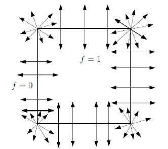
Figure 2.1. The function $f=\chi_{[0,1]^{2}}$ takes value $1$ on the unit square in $\mathbb{R}^{2}$ and $f(x)=0$ outside. The singular support, $\operatorname{sing\,supp}(f)$, is the boundary of the unit square. The directions of the ($C^{\infty}$) wavefront set of the function $f$ are shown with the arrows.

Sobolev wavefront sets have been used for studying pseudo-differential operators and non-linear partial differential operators. In particular, this concept helps to prove Hörmander’s propagation theorem, which characterizes the $C^{\infty}$ wavefront set of the distributional solution of a PDE using the principal symbol of the corresponding differential operator. Some basic properties of $C^{\infty}$ or Sobolev wavefront sets are given below (see [14, 23]) and are useful later in this paper.

Proposition 12.

For a distribution $f\in\mathcal{D}^{\prime}(\Omega)$,

$$\operatorname{WF}_{m}(f)\subseteq\operatorname{WF}_{n}(f)\subseteq\operatorname{WF}(f),\qquad\forall\;m\leq n$$

and $\operatorname{WF}(f)$ is the complement of the interior of $\cap_{m\in\mathbb{R}}(\operatorname{WF}_{m}(f)^{c})$, more precisely,

$$\operatorname{WF}(f)^{c}=\left(\bigcap_{m\in\mathbb{R}}\left(\operatorname{WF}_{m}(f)^{c}\right)\right)^{o},$$

where the superscript $o$ stands for the interior of a set.

3. Continuous shearlet transform in Sobolev spaces

To prove Theorems 3 and 4 for characterizing Sobolev wavefront sets through the continuous shearlet transform, we need to study the continuous shearlet transform $\mathcal{SH}_{\psi}f(a,s,t)$ in the Sobolev space $H^{m}(\mathbb{R}^{2})$ with $m\in\mathbb{R}$. We now extend the continuous shearlet transform from $L^{2}(\mathbb{R}^{2})$ to the Sobolev space $H^{m}(\mathbb{R}^{2})$ for tempered distributions.

Let $\mathbb{R}_{+}:=(0,\infty)$. The shearlet group $\left(\mathbb{R}_{+}\times\mathbb{R}\right)\times\mathbb{R}^{2}$ is equipped with a group multiplication: $(a,s,t)\cdot(a^{\prime},s^{\prime},t^{\prime})=(aa^{\prime},s+s^{\prime}\sqrt{a},t+M_{as}t)$. It has been studied by many researchers (e.g., [18]) that for every $f\in L^{2}(\mathbb{R}^{2})$,

(3.1) $$f(\cdot)=\int_{\mathbb{R}_{+}}\int_{\mathbb{R}}\int_{\mathbb{R}^{2}}\langle f,\psi_{ast}\rangle\psi_{ast}(\cdot)a^{-3}dtdsda$$

holds in the weak sense under the admissibility condition of the function $\psi$:

(3.2) $$\int_{\mathbb{R}_{+}}\int_{\mathbb{R}}\left|\widehat{\psi}\left(M_{as}^{T}\xi\right)\right|^{2}a^{-3/2}dsda=1,$$

where $M_{as}$ and $\psi_{ast}$ are defined in (1.4) and (1.5). Let $\psi$ be defined in (1.2), i.e., $\widehat{\psi}(\xi_{1},\xi_{2}):=\widehat{\psi_{1}}(\xi_{1})\widehat{\psi_{2}}(\xi_{2}/\xi_{1})$ with $\psi_{1},\psi_{2}$ satisfying the conditions in (C1) and (C2) in Subsection 1.1. Then it is well known that (3.2) holds. Indeed, by $\det(M_{as})=a^{3/2}$ and $\widehat{\psi}(M_{as}^{T}\xi)=\widehat{\psi_{1}}(a\xi_{1})\widehat{\psi_{2}}(\frac{1}{\sqrt{a}}(\frac{\xi_{2}}{\xi_{1}}-s))$, we have

$$\int_{\mathbb{R}_{+}}\int_{\mathbb{R}}|\widehat{\psi}(M_{as}^{T}\xi)|^{2}a^{-3/2}dsda=\int_{\mathbb{R}_{+}}\int_{\mathbb{R}}|\widehat{\psi_{1}}(a\xi_{1})|^{2}|\widehat{\psi_{2}}(\tfrac{1}{\sqrt{a}}(\tfrac{\xi_{2}}{\xi_{1}}-s))|^{2}a^{-3/2}dsda=1,$$

where we used the assumptions $\|\widehat{\psi_{2}}\|_{L^{2}}=1$ and (1.3) in (C1) and (C2).

Since $\psi$ is a Schwartz function, $\mathcal{SH}_{\psi}f(a,s,t):=\langle f,\psi_{ast}\rangle$ is well defined for any tempered distribution $f$. By (1.5), we have $\psi_{ast}=a^{-3/4}\psi(M_{as}^{-1}(\cdot-t))$ and hence

(3.3) $$\widehat{\psi_{ast}}(\xi)=a^{3/4}e^{-i2\pi t\cdot\xi}\widehat{\psi}(M_{as}^{T}\xi).$$

Therefore, by $\mathcal{SH}_{\psi}f(a,s,\cdot)=\langle f,\psi_{as\cdot}\rangle=a^{-3/4}f*\overline{\psi(-M_{as}^{-1}\cdot)}$, we obtain

(3.4) $$\left(\mathcal{SH}_{\psi}f(a,s,\cdot)\right)^{\wedge}(\xi)=a^{{3}/{4}}\widehat{f}(\xi)\overline{\widehat{\psi}\left(M_{as}^{T}\xi\right)}.$$

Since $\operatorname{supp}(\widehat{\psi})\subseteq\{(\xi_{1},\xi_{2})\;:\;1/2\leq|\xi_{1}|\leq 2,|\xi_{2}/\xi_{1}|\leq 1\}$, using (3.3), we obtain

(3.5) $$\operatorname{supp}(\widehat{\psi_{ast}})=\operatorname{supp}(\widehat{\psi}(M_{as}^{T}\cdot))=M_{as}^{-T}\operatorname{supp}(\widehat{\psi})\subseteq\Xi(a,s),$$

where $\Xi(a,s)$ is defined in (2.4). For $(a,s)\not\in(0,1]\times[-2,2]$, we have either $a>1$ or $|s|>2$. Let $(\xi_{1},\xi_{2})\in\Xi(a,s)$. If $a>1$, then $|\xi_{1}|<2$ and therefore, $(\xi_{1},\xi_{2})\not\in\mathcal{C}$, where the cone $\mathcal{C}$ is defined in (1.6). If $|s|>2$ and $0<a\leq 1$, then $|\xi_{2}/\xi_{1}|\geq|s|-\sqrt{a}>1$ and hence, $(\xi_{1},\xi_{2})\not\in\mathcal{C}$. This proves

(3.6) $$\widehat{\psi_{ast}}(\xi)=0=\widehat{\psi}\left(M_{as}^{T}\xi\right),\qquad\forall\;\xi\in\mathcal{C}\quad\mbox{and}\quad(a,s)\not\in(0,1]\times[-2,2].$$

Our main goal in this section is to develop some theory and estimate for the continuous shearlet transform in the Sobolev space $H^{m}(\mathbb{R}^{2})$ with any real number $m\in\mathbb{R}$. Firstly, since $\widehat{\psi}$ in Subsection 1.1 belongs to $\mathcal{D}(\mathbb{R}^{2})$, the shearlet $\psi_{ast}$ defined in (1.5) and all its derivatives are Schwartz functions with rapid decay at infinity. Hence, $\langle f,\psi_{ast}\rangle$ is well defined for every tempered distribution $f$ on $\mathbb{R}^{2}$. Now, we define a continuous shearlet transform (CST) associated to $\psi$ (defined in Subsection 1.1) as

$$\mathcal{SH}_{\psi}:H^{m}(\mathbb{R}^{2})\rightarrow L^{2}\left(\left(\mathbb{R}_{+}\times\mathbb{R},a^{-3}dsda\right),H^{m}(\mathbb{R}^{2})\right),$$

by

$$\mathcal{SH}_{\psi}f(a,s,t):=\left\langle f,\psi_{ast}\right\rangle,\ \mbox{for}\ f\in H^{m}(\mathbb{R}^{2})\ \mbox{and}\ (a,s,t)\in\left(\mathbb{R}_{+}\times\mathbb{R}\right)\times\mathbb{R}^{2}.$$

Here, the space $L^{2}((\mathbb{R}_{+}\times\mathbb{R},a^{-3}dsda),H^{m}(\mathbb{R}^{2}))$ is a fiber space, which is abbreviated by $\mathcal{F}^{m}$. Note that $\mathcal{F}^{m}$ is isomorphic to the tensor product $L^{2}(\mathbb{R}_{+}\times\mathbb{R},a^{-3}dsda)\widehat{\otimes}$ $H^{m}(\mathbb{R}^{2})$. The associated norm of $\mathcal{SH}_{\psi}f$ on the fiber space $\mathcal{F}^{m}$ is then defined by

$$\left\|\mathcal{SH}_{\psi}f\right\|_{\mathcal{F}^{m}}:=\left(\int_{a\in\mathbb{R}_{+}}\int_{s\in\mathbb{R}}\left\|\mathcal{SH}_{\psi}f(a,s,\cdot)\right\|_{H^{m}}^{2}a^{-3}dsda\right)^{{1}/{2}}.$$

The extended CST from $L^{2}(\mathbb{R}^{2})$ to $H^{m}(\mathbb{R}^{2})$ with $m\in\mathbb{R}$ leads to a unitary operator between the Sobolev space $H^{m}(\mathbb{R}^{2})$ and the fiber space $\mathcal{F}^{m}$. Some properties of the extended CST in the Sobolev space $H^{m}(\mathbb{R}^{2})$ are as follows:

Proposition 13.

For $f\in H^{m}(\mathbb{R}^{2})$ with $m\in\mathbb{R}$, the following statements hold:

1. For every fixed $a\in\mathbb{R}_{+}$ and $s\in\mathbb{R}$, the mapping $\mathcal{SH}_{\psi}f(a,s,\cdot)$ can be extended uniquely into a continuous mapping from $H^{m}(\mathbb{R}^{2})$ to itself.

2. $\mathcal{SH}_{\psi}$ is an isometry from $H^{m}(\mathbb{R}^{2})$ to $\mathcal{F}^{m}$, i.e., $\|\mathcal{SH}_{\psi}f\|_{\mathcal{F}^{m}}=\|f\|_{H^{m}}$.

Proof.

(i) By (3.4) and the definition of $H^{m}(\mathbb{R}^{2})$, we deduce that

$$\left\|\mathcal{SH}_{\psi}f(a,s,\cdot)\right\|_{H^{m}}^{2}=a^{{3}/{2}}\int_{\mathbb{R}^{2}}(1+|\xi|^{2})^{m}|\widehat{f}(\xi)|^{2}\left|\widehat{\psi}\left(M_{as}^{T}\xi\right)\right|^{2}d\xi,$$

from which we straightforwardly have $\left\|\mathcal{SH}_{\psi}f(a,s,\cdot)\right\|_{H^{m}}^{2}\leq a^{{3}/{2}}\|\widehat{\psi}\|_{L^{\infty}}^{2}\|f\|_{H^{m}}^{2}$.

(ii) Using (3.4) and Fubini’s theorem, by the admissibility condition in (3.2), we have

$$\left\|\mathcal{SH}_{\psi}f\right\|_{\mathcal{F}^{m}}^{2} =\int_{\mathbb{R}_{+}}\int_{\mathbb{R}}\left\|\mathcal{SH}_{\psi}f(a,s,\cdot)\right\|_{H^{m}}^{2}a^{-3}dsda$$

$$=\int_{\mathbb{R}^{2}}\left(\int_{\mathbb{R}_{+}}\int_{\mathbb{R}}a^{{3}/{2}}\left|\widehat{\psi}\left(M_{as}^{T}\ \xi\right)\right|^{2}a^{-3}dsda\right)(1+|\xi|^{2})^{m}|\widehat{f}(\xi)|^{2}d\xi$$

$$=\int_{\mathbb{R}^{2}}(1+|\xi|^{2})^{m}|\widehat{f}(\xi)|^{2}d\xi=\|f\|_{H^{m}}^{2}.$$

This completes the proof. ∎

The above result is established where the dilation and direction parameters $a$ and $s$ vary on the non-compact sets $\mathbb{R}_{+}$ and $\mathbb{R}$, respectively. Now, our aim is to obtain the above result for the Sobolev space $H^{m}(\mathbb{R}^{2})$ when both the parameters $a$ and $s$ vary on compact sets. Let $\mathcal{C}$ be the horizontal cone defined in (1.6). By switching $\xi_{1}$ with $\xi_{2}$, we define the vertical cone $\mathcal{C}^{v}:=\{(\xi_{2},\xi_{1})\;:\;(\xi_{1},\xi_{2})\in\mathcal{C}\}$. Consider the subspace $H^{m}(\mathcal{C})^{\vee}$ of $H^{m}(\mathbb{R}^{2})$ over the horizontal cone $\mathcal{C}$ as follows:

$$H^{m}(\mathcal{C})^{\vee}:=\{f\in H^{m}(\mathbb{R}^{2})\;:\;\operatorname{supp}(\widehat{f})\subseteq\mathcal{C}\}.$$

Similarly, we define $H^{m}(\mathcal{C}^{v})^{\vee}:=\{f\in H^{m}(\mathbb{R}^{2})\;:\;\operatorname{supp}(\widehat{f})\subseteq\mathcal{C}^{v}\}$ over $\mathcal{C}^{v}$. Let $R_{0}:=(0,1]\times[-2,2]$. We define the fiber spaces

$$\mathcal{F}^{m}_{\mathcal{C}}:=L^{2}((R_{0},a^{-3}dsda),H^{m}(\mathcal{C})^{\vee})\quad\mbox{and}\quad\mathcal{F}^{m}_{\mathcal{C}^{v}}:=L^{2}((R_{0},a^{-3}dsda),H^{m}(\mathcal{C}^{v})^{\vee}).$$

Now we establish the following result on restricting the continuous shearlet transform $\mathcal{SH}_{\psi}$ on the Sobolev subspaces $H^{m}(\mathcal{C})^{\vee}$ and $H^{m}(\mathcal{C}^{v})^{\vee}$.

Proposition 14.

The following identities are satisfied

(3.7) $$\|\mathcal{SH}_{\psi}f\|_{\mathcal{F}^{m}_{\mathcal{C}}}^{2}=\|f\|_{H^{m}}^{2}=\|\mathcal{SH}_{\psi}f\|_{\mathcal{F}^{m}}^{2},\qquad\forall\,f\in H^{m}(\mathcal{C})^{\vee}$$

and

$$\|\mathcal{SH}_{\psi}^{(v)}f\|_{\mathcal{F}^{m}_{\mathcal{C}^{v}}}^{2}=\|f\|_{H^{m}}^{2}=\|\mathcal{SH}_{\psi}^{(v)}f\|_{\mathcal{F}^{m}}^{2},\qquad\forall\,f\in H^{m}(\mathcal{C}^{v})^{\vee}.$$

Proof.

For $\xi\not\in\mathcal{C}$, by $\widehat{f}(\xi)=0$ and (3.4), we have $(\mathcal{SH}_{\psi}f(a,s,\cdot))^{\wedge}(\xi)=0$. For $\xi\in\mathcal{C}$ but $(a,s)\not\in I_{0}:=(0,1]\times[-2,2]$, it follows directly from (3.6) that $(\mathcal{SH}_{\psi}f(a,s,\cdot))^{\wedge}(\xi)=0$. Thus, it is now trivial to conclude that $\|\mathcal{SH}_{\psi}f\|_{\mathcal{F}^{m}_{\mathcal{C}}}^{2}=\|\mathcal{SH}_{\psi}f\|_{\mathcal{F}^{m}}^{2}$ for all $f\in H^{m}(\mathcal{C})^{\vee}$. Since we already proved $\|\mathcal{SH}_{\psi}f\|_{\mathcal{F}^{m}}^{2}=\|f\|_{H^{m}}^{2}$ in item (ii) of Proposition 13, this proves (3.7). ∎

The above result shows that a function $f$ in $H^{m}(\mathcal{C})^{\vee}$(or $H^{m}(\mathcal{C}^{v})^{\vee}$) can be continuously reproduced by using the continuous horizontal (or vertical) shearlet transform, but neither of them is sufficient to produce all $f\in H^{m}(\mathbb{R}^{2})$. To overcome this problem, noting that $\mathbb{R}^{2}=\tiny{\Box}\cup\mathcal{C}\cup\mathcal{C}^{v}$ with $\tiny{\Box}:=[-2,2]^{2}$, we decompose $f$ as follows:

(3.8) $$f=P_{\tiny{\Box}}f+P_{\mathcal{C}}f+P_{\mathcal{C}^{v}}f\quad\mbox{with}\quad\widehat{P_{\tiny{\Box}}f}=\widehat{f}\chi_{\tiny{\Box}},\quad\widehat{P_{\mathcal{C}}f}=\widehat{f}\chi_{\mathcal{C}},\quad\widehat{P_{\mathcal{C}^{v}}f}=\widehat{f}\chi_{\mathcal{C}^{v}}.$$

As a direct consequence of Proposition 14, we have

Theorem 15.

For every $f\in H^{m}(\mathbb{R}^{2})$ with $m\in\mathbb{R}$, the following identity holds:

$$\|f\|_{H^{m}}^{2}=\|P_{\tiny{\Box}}f\|_{H^{m}}^{2}+\left\|\mathcal{SH}_{\psi}(P_{\mathcal{C}}f)\right\|_{\mathcal{F}^{m}}^{2}+\left\|\mathcal{SH}_{\psi}^{v}(P_{\mathcal{C}^{v}}f)\right\|_{\mathcal{F}^{m}}^{2}.$$

Proof.

Since $\mathbb{R}^{2}$ is an almost disjoint union of $\tiny{\Box}$, $\mathcal{C}$ and $\mathcal{C}^{v}$, by definition, we have $\|f\|_{H^{m}}^{2}=\|P_{\tiny{\Box}}f\|_{H^{m}}^{2}+\|P_{\mathcal{C}}f\|_{H^{m}}^{2}+\|P_{\mathcal{C}^{v}}f\|_{H^{m}}^{2}$. Now the claim follows directly from Proposition 14. ∎

Note that the reproducing formula [18, (3.7)] holds as a corollary of Theorem 15 for $f\in H^{m}(\mathbb{R}^{2})$ with $m=0$.

4. Proofs of Theorems 3 and 4

In this section we shall prove Theorems 3 and 4, which address the relationship between the continuous shearlet transform and microlocal properties of a distribution. So we will perform microlocal analysis using the continuous shearlet transform.

According to Lemma 9, to prove Theorem 3, we have to find suitable conditions on which the microlocal Sobolev integral $\int_{U_{\xi_{0},\epsilon}}|\widehat{\varphi f}(\xi)|^{2}|\xi|^{2m}d\xi$ is finite. So, we now decompose the localized function $\varphi f$. Using the reproducing formula in (3.1) and noting $\mathcal{SH_{\psi}}(\varphi f)(a,s,t)=\langle\varphi f,\psi_{ast}\rangle$, we have

$$\widehat{\varphi f}(\xi)=\int_{\mathbb{R}_{+}}\int_{\mathbb{R}}\int_{\mathbb{R}^{2}}\widehat{\psi_{ast}}(\xi)\mathcal{SH}_{\psi}(\varphi f)(a,s,t)a^{-3}dtdsda.$$

Now by (3.6), if $\xi\in\mathcal{C}$, then $\widehat{\psi_{ast}}(\xi)=0$ for all $(a,s)\not\in(0,1]\times[-2,2]$. Therefore,

$$\widehat{\varphi f}(\xi)\chi_{\mathcal{C}}(\xi)=\chi_{\mathcal{C}}(\xi)\int_{a=0}^{a=1}\int_{s=-2}^{s=2}\int_{t\in\mathbb{R}^{2}}\widehat{\psi_{ast}}(\xi)\mathcal{SH}_{\psi}(\varphi f)(a,s,t)a^{-3}dtdsda.$$

Consequently, we have the following decomposition:

$$(\widehat{\varphi f})(\xi)= (\widehat{P_{\tiny{\Box}}(\varphi f)})(\xi)+\chi_{\mathcal{C}}(\xi)\int_{a=0}^{a=1}\int_{s=-2}^{s=2}\int_{t\in\mathbb{R}^{2}}\widehat{\psi_{ast}}(\xi)\mathcal{SH}_{\psi}(\varphi f)(a,s,t)a^{-3}dtdsda$$

(4.1) $$+\chi_{\mathcal{C}^{v}}(\xi)\int_{a=0}^{a=1}\int_{s=-2}^{s=2}\int_{t\in\mathbb{R}^{2}}\widehat{\psi^{(v)}_{ast}}(\xi)\mathcal{SH}_{\psi}^{(v)}(\varphi f)(a,s,t)a^{-3}dtdsda.$$

Let $x_{0}\in\mathbb{R}^{2}$ and $\xi_{0}\in\mathbb{R}^{2}\backslash\{0\}$. We define $s_{0}:=\tan(\mbox{Arg}(\xi_{0}))$, which is just the slope of the direction $\xi_{0}$. For small $\epsilon>0$, we observe that

(4.2) $$U_{\pm\xi_{0},\epsilon}\subseteq\left\{\tfrac{1}{a}(\cos(\arctan s),\sin(\arctan s))\;:\;|a|\in(0,1),|s-s_{0}|<r_{0}\right\}=:W_{s_{0},r_{0}},$$

where

(4.3) $$r_{0}:=\max(\tan(\mbox{Arg}(\xi_{0})+\epsilon)-s_{0},s_{0}-\tan(\mbox{Arg}(\xi_{0})-\epsilon))>0.$$

Note that $r_{0}\to 0^{+}$ as $\epsilon\to 0^{+}$. Define $N_{r_{0}}(s_{0},x_{0}):=I_{s_{0}}\times B_{r_{0}}(x_{0})$, where

$$I_{s_{0}}:=[-2,2]\cap[s_{0}-2r_{0},s_{0}+2r_{0}].$$

Then the decomposition in (4) can be rewritten as

(4.4) $$(\widehat{\varphi f})(\xi)=(\widehat{P_{\tiny{\Box}}(\varphi f)})(\xi)+\widehat{g_{1}}(\xi)+\widehat{g_{2}}(\xi)+\widehat{g_{3}}(\xi)+\widehat{g_{4}}(\xi),$$

where

(4.5) $$\widehat{g_{1}}(\xi):=\chi_{\mathcal{C}}(\xi)\int_{a=0}^{a=1}\int_{(s,t)\in I_{s_{0}}\times B_{r_{0}}(x_{0})}\widehat{\psi_{ast}}(\xi)\mathcal{SH}_{\psi}(\varphi f)(a,s,t)a^{-3}dsdtda$$

and

$$\widehat{g_{2}}(\xi):=\chi_{\mathcal{C}}(\xi)\int_{a=0}^{a=1}\int_{(s,t)\in([-2,2]\times\mathbb{R}^{2})\backslash N_{r_{0}}(s_{0},x_{0})}\widehat{\psi_{ast}}(\xi)\mathcal{SH}_{\psi}(\varphi f)(a,s,t)a^{-3}dsdtda,$$

and $g_{3},g_{4}$ are similarly defined as $g_{1},g_{2}$ by exchanging $\mathcal{SH}_{\psi}$ with $\mathcal{SH}_{\psi}^{(v)}$, respectively.

Since $\widehat{\varphi f}$ is continuous and $\widehat{P_{\tiny{\Box}}(\varphi f)}(\xi)=\widehat{(\varphi f)}(\xi)\chi_{\tiny{\Box}}(\xi)$, by the definition of $U_{\xi_{0},\epsilon}$ in (2.2), it is trivial to conclude that

$$\int_{U_{\xi_{0},\epsilon}}|\widehat{P_{\tiny{\Box}}(\varphi f)}(\xi)|^{2}|\xi|^{2m}d\xi\leq\left(\sup_{\xi\in\tiny{\Box}}|\widehat{\varphi f}(\xi)|^{2}\right)\int_{U_{\xi_{0},\epsilon}\cap\tiny{\Box}}|\xi|^{2m}d\xi<\infty,$$

for all $\xi_{0}\in\mathbb{R}^{2}\backslash\{0\}$, $\epsilon>0$ and $m\in\mathbb{R}$.

We have the following result estimating $g_{2}$.

Proposition 16.

For all $\xi_{0}\in\mathbb{R}^{2}\backslash\{0\}$, $0<\epsilon<\pi/2$ and $m\in\mathbb{R}$,

$$\int_{U_{\pm\xi_{0},\epsilon}}|\widehat{g_{2}}(\xi)|^{2}|\xi|^{2m}d\xi<\infty.$$

Proof.

We decompose $([-2,2]\times\mathbb{R}^{2})\backslash N_{r_{0}}(s_{0},x_{0})=E_{1}\cup E_{2}$ with $E_{1}:=I_{s_{0}}^{c}\times\mathbb{R}^{2}$ and $E_{2}:=I_{s_{0}}\times B_{r_{0}}(x_{0})^{c}$, where $I_{s_{0}}^{c}:=[-2,2]\backslash I_{s_{0}}$ and $B_{r_{0}}(x_{0})^{c}:=\mathbb{R}^{2}\backslash B_{r_{0}}(x_{0})$. We define $\widehat{h_{j}}:=\widehat{g_{2}}\chi_{E_{j}}$ for $j=1,2$. We first deal with $\int_{U_{\pm\xi_{0},\epsilon}}|\widehat{h_{1}}(\xi)|^{2}|\xi|^{2m}d\xi$. Note that

$$\widehat{h_{1}}(\xi)=\chi_{\mathcal{C}}(\xi)\int_{a=0}^{a=1}\int_{s\in I_{s_{0}}^{c}}\int_{t\in\mathbb{R}^{2}}\widehat{\psi_{ast}}(\xi)\mathcal{SH}_{\psi}(\varphi f)(a,s,t)a^{-3}dtdsda.$$

By (3.3), we have

$$\int_{\mathbb{R}^{2}}\widehat{\psi_{ast}}(\xi)\mathcal{SH}_{\psi}(\varphi f)(a,s,t)dt=a^{3/4}\widehat{\psi}(M_{as}^{T}\xi)(\mathcal{SH}_{\psi}(\varphi f)(a,s,\cdot))^{\wedge}(\xi).$$

Hence, by (3.4), we conclude that

$$|\widehat{h_{1}}(\xi)|\leq\chi_{\mathcal{C}}(\xi)\int_{a=0}^{a=1}\int_{s\in I_{s_{0}}^{c}}|\widehat{\psi}(M_{as}^{T}\xi)|^{2}|\widehat{\varphi f}(\xi)|a^{-3/2}dsda.$$

By (4.2), we have $U_{\pm\xi_{0},\epsilon}\subseteq W_{s_{0},r_{0}}$. For $s\in I_{s_{0}}^{c}$ (which implies $|s-s_{0}|>2r_{0}$), then $\Xi(a,s)\cap W_{s_{0},r_{0}}=\emptyset$ for $0<\sqrt{a}<|s-s_{0}|-r_{0}$. For $s\in I_{s_{0}}^{c}$, by definition we have $|s-s_{0}|>2r_{0}$ which implies $|s-s_{0}|-r_{0}>r_{0}$. Then for $\xi\in U_{\pm\xi_{0},\epsilon}$, we deduce from (3.5) that

$$|\widehat{h_{1}}(\xi)|\leq\int_{a=r_{0}^{2}}^{a=1}\int_{s\in I_{s_{0}}^{c}}|\widehat{\psi}(M_{as}^{T}\xi)|^{2}|\widehat{\varphi f}(\xi)|a^{-3/2}dsda.$$

Since $0<r_{0}<1$, we see that

(4.6) $$K_{r_{0}}:=\cup_{a\in[r_{0}^{2},1],s\in[-2,2]}\Xi(a,s)\subseteq\{(\xi_{1},\xi_{2})\;:\;\tfrac{1}{2}\leq|\xi_{1}|\leq\tfrac{2}{r_{0}^{2}},|\tfrac{\xi_{2}}{\xi_{1}}|\leq 3\}$$

is a bounded set. Because $\widehat{\varphi f}$ is continuous, we conclude that $C:=\sup_{\xi\in K_{r_{0}}}|\widehat{\varphi f}(\xi)|<\infty$. So, for $\xi\in U_{\pm\xi_{0},\epsilon}$, by (3.5), we have

$$|\widehat{h_{1}}(\xi)|\leq C\|\widehat{\psi}\|^{2}_{L^{\infty}}\int_{a=r_{0}^{2}}^{a=1}\int_{s\in I_{s_{0}}^{c}}\chi_{\Xi(a,s)}(\xi)a^{-3/2}dsda.$$

Note that $\Xi(a,s)\subseteq K_{r_{0}}$ for all $a\in[r_{0}^{2},1]$ and $s\in I_{s_{0}}^{c}$. Therefore, for $\xi\in U_{\pm\xi_{0},\epsilon}$, by (4.6), we have

$$|\widehat{h_{1}}(\xi)|\leq C\|\widehat{\psi}\|^{2}_{L^{\infty}}\int_{a=r_{0}^{2}}^{a=1}\int_{s\in I_{s_{0}}^{c}}\chi_{K_{r_{0}}}(\xi)a^{-3/2}dsda\leq C_{1}\chi_{K_{r_{0}}}(\xi),$$

where $C_{1}=8C\|\widehat{\psi}\|^{2}_{L^{\infty}}(r_{0}^{-1}-1)$. Consequently, by $U_{\pm\xi_{0},\epsilon}\subseteq W_{s_{0},r_{0}}$ and (4.6),

$$\int_{U_{\pm\xi_{0},\epsilon}}|\widehat{h_{1}}(\xi)|^{2}|\xi|^{2m}d\xi \leq C_{1}\int_{U_{\pm\xi_{0},\epsilon}\cap K_{r_{0}}}|\xi|^{2m}d\xi\leq C_{1}\int_{K_{r_{0}}}|\xi|^{2m}d\xi$$

$$\leq C_{1}\int_{\theta=-\arctan 3}^{\theta=\arctan 3}\int_{r=1/2}^{r=\frac{2\sqrt{1+3^{2}}}{r_{0}^{2}}}r^{2m+1}drd\theta<\infty.$$

Finally, we show $\int_{U_{\pm\xi_{0},\epsilon}}|\widehat{h_{2}}(\xi)|^{2}|\xi|^{2m}d\xi<\infty$. First note that

$$\widehat{h_{2}}(\xi)=\chi_{\mathcal{C}}(\xi)\int_{a=0}^{a=1}\int_{s\in I_{s_{0}}}\int_{t\in B_{r_{0}}(x_{0})^{c}}\widehat{\psi_{ast}}(\xi)\mathcal{SH}_{\psi}(\varphi f)(a,s,t)a^{-3}dtdsda.$$

By [18, Lemma 5.2] for each $k>0$, there exists a positive constant $C_{2}$ such that

(4.7) $$|\mathcal{SH}_{\psi}(\varphi f)(a,s,t)|=|\left\langle\varphi f,\psi_{ast}\right\rangle|\leq C_{2}a^{\frac{1}{4}}\left(1+\frac{d(t,B_{r_{0}^{\prime}}(x_{0}))^{2}}{a}\right)^{-k},$$

for all $a\in(0,1]$, $s\in[-2,2]$ and $t\in\mathbb{R}^{2}$, where $\operatorname{supp}(\varphi)\subseteq B_{r_{0}^{\prime}}(x_{0})\subseteq B_{r_{0}}(x_{0})\subseteq\Omega$ with $0<r_{0}^{\prime}<r_{0}$. Using (3.3), (3.5) and (4.7), we get

$$| \widehat{h_{2}}(\xi)|\leq\chi_{\mathcal{C}}(\xi)\int_{a=0}^{a=1}\int_{s\in I_{s_{0}}}\int_{t\in B_{r_{0}}(x_{0})^{c}}|\widehat{\psi_{ast}}(\xi)||\mathcal{SH}_{\psi}(\varphi f)(a,s,t)|a^{-3}dtdsda$$

$$\leq C_{2}\|\widehat{\psi}\|_{L^{\infty}}\int_{0}^{1}\int_{I_{s_{0}}}\int_{B_{r_{0}}(x_{0})^{c}}a^{\tfrac{3}{4}}\chi_{\Xi(a,s)}(\xi)a^{\tfrac{1}{4}}\left(1+\frac{d(t,B_{r_{0}^{\prime}}(x_{0}))^{2}}{a}\right)^{-k}a^{-3}dtdsda$$

$$\leq C_{2}\|\widehat{\psi}\|_{L^{\infty}}\int_{0}^{1}\left(\int_{I_{s_{0}}}\chi_{\Xi(a,s)}(\xi)ds\right)\left(\int_{B_{r_{0}}(x_{0})^{c}}\left(1+\frac{d(t,B_{r_{0}^{\prime}}(x_{0}))^{2}}{a}\right)^{-k}dt\right)a^{-2}da.$$

For $\xi\in\Xi(a,s),s\in[-2,2]$ and $a\in(0,1)$, we observe

(4.8) $$\tfrac{1}{\sqrt{2}}\leq\tfrac{\sqrt{1+(|s|-\sqrt{a})^{2}}}{2}<a|\xi|<2\sqrt{1+(|s|+\sqrt{a})^{2}}\leq 2\sqrt{10}.$$

For $a\in(0,1)$ such that $a\not\in[\frac{1}{\sqrt{2}|\xi|},\frac{2\sqrt{10}}{|\xi|}]$, then the above inequality implies $\xi\not\in\Xi(a,s)$ for all $s\in[-2,2]$, which leads to $\int_{I_{s_{0}}}\chi_{\Xi(a,s)}(\xi)ds=0$. Note that $\xi\in\Xi(a,s)$ implies $\frac{\xi_{2}}{\xi_{1}}-\sqrt{a}\leq s\leq\frac{\xi_{2}}{\xi_{1}}+\sqrt{a}$. Consequently, we conclude that $\int_{I_{s_{0}}}\chi_{\Xi(a,s)}(\xi)ds\leq 2\sqrt{a}\chi_{[\frac{1}{\sqrt{2}|\xi|},\frac{2\sqrt{10}}{|\xi|}]}(a)$. Therefore, for $k>1$,

$$|\widehat{h_{2}}(\xi)| \leq 2C_{2}\|\widehat{\psi}\|_{L^{\infty}}\int_{a=\tfrac{1}{\sqrt{2}|\xi|}}^{a=\tfrac{2\sqrt{10}}{|\xi|}}\int_{t\in B_{r_{0}}(x_{0})^{c}}\left(1+\frac{d(t,B_{r_{0}^{\prime}}(x_{0}))^{2}}{a}\right)^{-k}a^{-\tfrac{3}{2}}dtda$$

$$=4\pi C_{2}\|\widehat{\psi}\|_{L^{\infty}}\int_{a=\tfrac{1}{\sqrt{2}|\xi|}}^{a=\tfrac{2\sqrt{10}}{|\xi|}}\left(\int_{r=r_{0}-r_{0}^{\prime}}^{\infty}\left(1+a^{-1}r^{2}\right)^{-k}rdr\right)a^{-\tfrac{3}{2}}da$$

$$=\frac{2\pi C_{2}\|\widehat{\psi}\|_{L^{\infty}}}{k-1}\int_{a=\tfrac{1}{\sqrt{2}|\xi|}}^{a=\tfrac{2\sqrt{10}}{|\xi|}}a^{-\tfrac{1}{2}}\left(1+a^{-1}(r_{0}-r_{0}^{\prime})^{2}\right)^{-k+1}da$$

$$\leq C_{3}|\xi|^{-\tfrac{1}{2}}\left(1+\frac{|\xi|}{2\sqrt{10}}(r_{0}-r_{0}^{\prime})^{2}\right)^{-k+1},$$

where $C_{3}:=\frac{(4\sqrt{5}-1)\pi C_{2}\|\widehat{\psi}\|_{L^{\infty}}}{2^{1/4}(k-1)}<\infty$ for $k>1$. Consequently, taking $k>\max(m+2,1)$, we conclude that $\int_{U_{\pm\xi_{0},\epsilon}}|\widehat{h_{2}}(\xi)|^{2}|\xi|^{2m}d\xi<\infty$. ∎

The same technique in the proof of Proposition 16 for estimating $g_{2}$ can be applied to estimate $g_{4}$ for the vertical shearlet coefficients as well. We now estimate $\int_{U_{\pm\xi_{0},\epsilon}}|\widehat{g_{1}}(\xi)|^{2}|\xi|^{2m}d\xi$ as follows. The same technique can be used to estimate $g_{3}$.

Proposition 17.

There exists a positive constant $c$ such that

(4.9) $$\int_{U_{\pm\xi_{0},\epsilon}}|\widehat{g_{1}}(\xi)|^{2}|\xi|^{2m}d\xi\leq c\int_{a=0}^{a=1}\int_{s\in I_{s_{0}}}\int_{t\in B_{r_{0}}(x_{0})}\left|\mathcal{SH}_{\psi}(\varphi f)(a,s,t)\right|^{2}a^{-2m-3}dtdsda,$$

where $s_{0}:=\tan(\mbox{Arg}(\xi_{0}))$ and $r_{0}$ is defined in (4.3).

Proof.

To prove (4.9), by the definition of $\widehat{g_{1}}$ in (4.5), for $\xi\in U_{\pm\xi_{0},\epsilon}$, we get

$$\widehat{g_{1}}(\xi)|\xi|^{m}=\chi_{\mathcal{C}}(\xi)\int_{a=0}^{a=1}\int_{s\in I_{s_{0}}}\int_{t\in B_{r_{0}}(x_{0})}(a|\xi|)^{m}\widehat{\psi_{ast}}(\xi)\mathcal{SH}_{\psi}(\varphi f)(a,s,t)a^{-m-3}dsdtda$$

$$=\chi_{\mathcal{C}}(\xi)\int_{a=0}^{a=1}\int_{s\in I_{s_{0}}}\int_{t\in B_{r_{0}}(x_{0})}\mathcal{SH}_{\psi}(\varphi f)(a,s,t)a^{-m}e^{-2\pi i\xi\cdot t}(a|\xi|)^{m}\widehat{\psi_{as0}}(\xi)a^{-3}dsdtda$$

$$=\chi_{\mathcal{C}}(\xi)\int_{a=0}^{a=1}\left(\int_{s\in I_{s_{0}}}\widehat{A}(a,s,\xi)(a|\xi|)^{m}\widehat{\psi_{as0}}(\xi)a^{-2}ds\right)\frac{da}{a},$$

where we define

$$\widehat{A}(a,s,\xi):=\int_{t\in B_{r_{0}}(x_{0})}\mathcal{SH}_{\psi}(\varphi f)(a,s,t)a^{-m}e^{-2\pi i\xi\cdot t}dt,$$

which is just the Fourier transform of $\chi_{B_{r_{0}}(x_{0})}(\cdot)\mathcal{SH}_{\psi}(\varphi f)(a,s,\cdot)a^{-m}$. Because the function $\widehat{\psi_{1}}$ is supported inside $[-2,-\frac{1}{2}]\cup[\frac{1}{2},2]$, we observe that

$$\widehat{\psi_{1}}(a\xi_{1})=\widehat{\psi_{1}}(a\xi_{1})\chi_{J_{\xi}}(a)\quad\mbox{with}\quad J_{\xi}:=[\tfrac{1}{2|\xi_{1}|},\tfrac{2}{|\xi_{1}|}].$$

Using (1.2) and (3.3), we obtain

$$\widehat{g_{1}}(\xi)|\xi|^{m} =\chi_{\mathcal{C}}(\xi)\int_{a=0}^{a=1}a^{-\frac{3}{4}}(a|\xi|)^{m}\widehat{\psi_{1}}(a\xi_{1})\chi_{J_{\xi}}(a)\widehat{\mathcal{A}}(a,\xi)\frac{da}{a},$$

where $\widehat{\mathcal{A}}(a,\xi):=\int_{s\in I_{s_{0}}}\widehat{A}(a,s,\xi)\widehat{\psi_{2}}\left(a^{-\frac{1}{2}}\left(\frac{\xi_{2}}{\xi_{1}}-s\right)\right)a^{-\frac{1}{2}}ds$. Hence, for $\xi=(\xi_{1},\xi_{2})\in U_{\pm\xi_{0},\epsilon}$, we get

$$|\widehat{g_{1}}(\xi)|^{2}|\xi|^{2m} \leq \chi_{\mathcal{C}}(\xi)\left(\int_{a\in(0,1)\cap J_{\xi}}\left|a^{-\frac{3}{4}}(a|\xi|)^{m}\widehat{\psi_{1}}(a\xi_{1})\widehat{\mathcal{A}}(a,\xi)\right|\frac{da}{a}\right)^{2}$$

$$\leq \chi_{\mathcal{C}}(\xi)\left(\int_{a\in(0,1)\cap J_{\xi}}\left|a^{-\frac{3}{4}}(a|\xi|)^{m}\widehat{\psi_{1}}(a\xi_{1})\widehat{\mathcal{A}}(a,\xi)\right|^{2}\frac{da}{a}\right)\left(\int_{\frac{1}{2|\xi_{1}|}}^{\frac{2}{|\xi_{1}|}}\frac{da}{a}\right)$$

$$= (\log 4)\chi_{\mathcal{C}}(\xi)\left(\int_{a\in(0,1)\cap J_{\xi}}\left|a^{-\frac{3}{4}}(a|\xi|)^{m}\widehat{\psi_{1}}(a\xi_{1})\widehat{\mathcal{A}}(a,\xi)\right|^{2}\frac{da}{a}\right).$$

By $\operatorname{supp}(\widehat{\psi_{2}})\subseteq[-1,1]$, defining $J_{\xi,a}:=\left[\frac{\xi_{2}}{\xi_{1}}-\sqrt{a},\frac{\xi_{2}}{\xi_{1}}+\sqrt{a}\right]$, we observe that

$$\widehat{\psi}_{2}\left(a^{-\frac{1}{2}}\left(\frac{\xi_{2}}{\xi_{1}}-s\right)\right)=\widehat{\psi}_{2}\left(a^{-\frac{1}{2}}\left(\frac{\xi_{2}}{\xi_{1}}-s\right)\right)\chi_{J_{\xi,a}}(s).$$

Also by $\|\widehat{\psi_{2}}\|_{L^{2}}=1$, we deduce that

$$\int_{s\in I_{s_{0}}}\left|\widehat{\psi}_{2}\left(a^{-\frac{1}{2}}\left(\frac{\xi_{2}}{\xi_{1}}-s\right)\right)\right|^{2}\frac{ds}{a}=a^{-\frac{1}{2}}\int_{s\in a^{-\frac{1}{2}}(\frac{\xi_{2}}{\xi_{1}}-I_{s_{0}})}|\widehat{\psi_{2}}(s)|^{2}ds\leq a^{-\frac{1}{2}}.$$

Using the Cauchy-Schwartz inequality and the definition of $\widehat{\mathcal{A}}(a,\xi)$, we have

$$\left|\widehat{\mathcal{A}}(a,\xi)\right|^{2} \leq\left(\int_{s\in I_{s_{0}}}\left|\widehat{\psi}_{2}\left(a^{-\frac{1}{2}}\left(\frac{\xi_{2}}{\xi_{1}}-s\right)\right)\right|^{2}\frac{ds}{a}\right)\left(\int_{s\in I_{s_{0}}}\left|\widehat{A}(a,s,\xi)\right|^{2}\chi_{J_{\xi,a}}(s)ds\right)$$

$$\leq a^{-\frac{1}{2}}\int_{s\in I_{s_{0}}\cap J_{\xi,a}}\left|\widehat{A}(a,s,\xi)\right|^{2}ds.$$

Therefore, we proved

$$|\widehat{g_{1}}(\xi)|^{2}|\xi|^{2m}\leq(\log 4)\chi_{\mathcal{C}}(\xi)\int_{a\in(0,1)\cap J_{\xi}}\int_{s\in I_{s_{0}}\cap J_{\xi,a}}(a|\xi|)^{2m}|\widehat{\psi_{1}}(a\xi_{1})|^{2}|\widehat{\mathcal{A}}(a,s,\xi)|^{2}a^{-3}dsda.$$

Note that $|\widehat{\psi_{1}}(a\xi_{1})|^{2}\chi_{J_{\xi,a}}(s)\leq\|\widehat{\psi_{1}}\|_{L^{\infty}}^{2}\chi_{\Xi(a,s)}(\xi)$. Using the inequality in (4.8), we have

(4.10) $$(a|\xi|)^{2m}\leq\max(2^{-m},40^{m}),\qquad\forall\,\xi\in\Xi(a,s),a\in(0,1),s\in[-2,2].$$

Putting all the above estimates together we obtain the following estimate

$$\int_{U_{\pm\xi_{0},\epsilon}}|\widehat{g_{1}}(\xi)|^{2}|\xi|^{2m}d\xi \leq c\int_{\xi\in U_{\pm\xi_{0},\epsilon}\cap\mathcal{C}}\int_{a\in(0,1)\cap J_{\xi}}\int_{s\in I_{s_{0}}\cap J_{\xi,a}}|\widehat{A}(a,s,\xi)|^{2}a^{-3}dsdad\xi$$

$$\leq c\int_{a=0}^{a=1}\int_{s\in I_{s_{0}}}\left(\int_{\xi\in\mathbb{R}^{2}}|\widehat{A}(a,s,\xi)|^{2}d\xi\right)a^{-3}dsda$$

$$=c\int_{a=0}^{a=1}\int_{s\in I_{s_{0}}}\int_{t\in B_{r_{0}}(x_{0})}|\mathcal{SH}_{\psi}(\varphi f)(a,s,t)(a,s,t)|^{2}a^{-2m-3}dtdsda,$$

where $c:=(\log 4)\|\widehat{\psi_{1}}\|_{L^{\infty}}^{2}\max(2^{-m},40^{m})$ and we noticed that $\widehat{A}(a,s,\xi)$ is the Fourier transform of $\chi_{B_{r_{0}}(x_{0})}(\cdot)\mathcal{SH}_{\psi}(\varphi f)(a,s,\cdot)a^{-m}$. This proves (4.9). ∎

To prove Theorem 3, we need the following two auxiliary results.

Lemma 18.

Let $f\in\mathcal{D}^{\prime}(\Omega)$ be a distribution and $x_{0}\in\Omega$. For any $r_{0}>0$ and a bounded interval $I_{s_{0}}$ of $[-2,2]$ such that $B_{r_{0}}(x_{0})\subseteq\Omega$, if $\varphi\in\mathcal{D}(\Omega)$ satisfies $\operatorname{supp}(\varphi)\subseteq B_{r_{0}}(x_{0})$, then

(4.11) $$\int_{a=0}^{a=1}\int_{s=s_{0}-r_{0}}^{s=s_{0}+r_{0}}\int_{t\in B_{r_{0}}(x_{0})}\left|\left\langle(1-\varphi)f,\psi_{ast}\right\rangle\right|^{2}a^{-2m-3}dtdsda<\infty.$$

Consequently, for $\varphi\in\mathcal{D}(\Omega)$ with $\operatorname{supp}(\varphi)\subseteq B_{r_{0}}(x_{0})$, the following two integrals

$$\int_{a=0}^{a=1}\int_{s\in I_{s_{0}}}\int_{t\in B_{r_{0}}(x_{0})}\left|\mathcal{SH}_{\psi}(\varphi f)(a,s,t)\right|^{2}a^{-2m-3}dtdsda$$

and

$$\int_{a=0}^{a=1}\int_{s\in I_{s_{0}}}\int_{t\in B_{r_{0}}(x_{0})}\left|\mathcal{SH}_{\psi}f(a,s,t)\right|^{2}a^{-2m-3}dtdsda$$

are either both finite (i.e., convergent) or both infinite (i.e., divergent).

Proof.

By [18, Lemma 5.2], for each $k>0$, there exists a positive constant $C$ depending on $k$ and satisfying

(4.12) $$|\langle(1-\varphi)f,\psi_{ast}\rangle|\leq Ca^{\frac{1}{4}}\left(1+\tfrac{\eta^{2}}{a}\right)^{-k}=Ca^{k+\frac{1}{4}}(a+\eta^{2})^{-k}\leq C\eta^{-2k}a^{k+\frac{1}{4}}$$

for all $a\in(0,1)$, $s\in[-2,2]$ and $t\in\mathbb{R}^{2}$, where $\eta=\mbox{dist}(B_{r_{0}}(x_{0}),(\operatorname{supp}\varphi)^{c})>0$. Hence, we get

$$\int_{a=0}^{a=1}\int_{s=s_{0}-r_{0}}^{s=s_{0}+r_{0}}\int_{t\in B_{r_{0}}(x_{0})}\left|\left\langle(1-\varphi)f,\psi_{ast}\right\rangle\right|^{2}a^{-2m-3}dtdsda\leq\frac{C^{2}}{\eta^{4k}}\int_{0}^{1}a^{2k-2m-\frac{5}{2}}da.$$

Note that the above last integral $\int_{0}^{1}a^{2k-2m-\frac{5}{2}}da<\infty$ if and only if $k>m+\frac{3}{4}$. Taking $k>\max(0,m+\frac{3}{4})$, we conclude that the integral in (4.11) is finite.

On the other hand, it is trivial that

(4.13) $$\mathcal{SH}_{\psi}f(a,s,t)=\langle f,\psi_{ast}\rangle=\langle\varphi f,\psi_{ast}\rangle+\langle(1-\varphi)f,\psi_{ast}\rangle.$$

Hence, using the inequality $(b+c)^{2}\leq 2b^{2}+2c^{2}$ for all $b,c\in\mathbb{R}$, we have

$$|\langle f,\psi_{ast}\rangle|^{2}\leq 2|\langle\varphi f,\psi_{ast}\rangle|^{2}+2|\langle(1-\varphi)f,\psi_{ast}\rangle|^{2}$$

and

$$|\langle\varphi f,\psi_{ast}\rangle|^{2}\leq 2|\langle f,\psi_{ast}\rangle|^{2}+2|\langle(1-\varphi)f,\psi_{ast}\rangle|^{2}.$$

Consequently, by (4.11), the two integrals are either both finite or both infinite. ∎

Lemma 19.

Let $f$ be a tempered distribution on $\mathbb{R}^{2}$. For $x_{0}\in\mathbb{R}^{2}$ and $s_{0}\in\mathbb{R}$,

(4.14) $$\int_{a=a_{0}}^{a=1}\int_{s=s_{0}-r_{0}}^{s=s_{0}+r_{0}}\int_{t\in B_{r_{0}}(x_{0})}\left|\mathcal{SH}_{\psi}f(a,s,t)\right|^{2}a^{-2m-3}dtdsda<\infty$$

for all $a_{0}>0$, $r_{0}>0$ and $m\in\mathbb{R}$.

Proof.

For all $a\in[a_{0},1)$ and $s\in(s_{0}-r_{0},s_{0}+r_{0})$, the support $\Xi(a,s)$ of $\widehat{\psi_{ast}}$ is contained inside a finite ball $B_{R}(0)$ for some $0<R<\infty$. Take $\eta\in\mathcal{D}(\mathbb{R}^{2})$ such that $\eta=1$ on $B_{R+1}(0)$. Therefore,

$$|\langle f,\psi_{ast}\rangle|=|\langle\eta f,\psi_{ast}\rangle|=|\langle\widehat{\eta f},\widehat{\psi_{ast}}\rangle|\leq Ca^{3/4}\quad\mbox{with}\quad C:=\|\widehat{\psi}\|_{L^{\infty}}\sup_{|\xi|\leq R}|\widehat{\eta f}(\xi)|<\infty,$$

since $\eta f$ is a compactly supported distribution and hence $\widehat{\eta f}$ is continuous. Therefore,

$$\int_{a=a_{0}}^{a=1} \int_{s=s_{0}-r_{0}}^{s=s_{0}+r_{0}}\int_{t\in B_{r_{0}}(x_{0})}|\langle f,\psi_{ast}\rangle|^{2}a^{-2m-3}dtdsda$$

$$\leq C^{2}\int_{a=a_{0}}^{a=1}\int_{s=s_{0}-r_{0}}^{s=s_{0}+r_{0}}\int_{t\in B_{r_{0}}(x_{0})}a^{-2m-3/2}dtdsda<\infty,$$

since $\int_{a=a_{0}}^{a=1}a^{-2m-3/2}da<\infty$ due to $a_{0}>0$. This proves (4.14). ∎

We are now ready to prove our main results in Theorems 3 and 4.

Proof of Theorem 3.

Sufficiency. Suppose that (1.11) or (1.12) holds at $(x_{0},\xi_{0})$ for some $r_{0}>0$. Since $s_{0}:=\tan(\mbox{Arg}(\xi_{0}))$, without loss of generality, we assume $|s_{0}|<2$ and (1.11) holds. By Proposition 16, Proposition 17 and Lemma 18, we deduce from (4.4) that (2.1) holds. Hence, by Lemma 9, $(x_{0},\pm\xi_{0})\not\in\operatorname{WF}_{m}(f)$.

Necessity. Suppose that $(x_{0},\pm\xi_{0})\not\in\operatorname{WF}_{m}(f)$. Note that $s_{0}:=\tan(\mbox{Arg}(\xi_{0}))$. Without loss of generality, we assume $|s_{0}|<2$. We have to prove (1.11). To do so, we first prove that

(4.15) $$\int_{a=0}^{a=1}\int_{s=s_{0}-r_{0}}^{s=s_{0}+r_{0}}\int_{t\in B_{r_{0}}(x_{0})}\left|\left\langle\varphi f,\psi_{ast}\right\rangle\right|^{2}a^{-2m-3}dtdsda<\infty.$$

Since $(x_{0},\pm\xi_{0})\not\in\operatorname{WF}_{m}(f)$, by Lemma 9, there exists $\epsilon>0$ such that (2.1) holds, that is, $C:=\int_{U}|\widehat{\varphi f}(\xi)|^{2}|\xi|^{2m}d\xi<\infty$, where $U:=U_{\xi_{0},\epsilon}\cup(-U_{\xi_{0},\epsilon})$. To prove (4.11), using the relation $\operatorname{supp}(\widehat{\psi_{ast}})\subseteq\Xi(a,s)$ in (3.5), we observe

$$\langle\varphi f,\psi_{ast}\rangle=\langle\widehat{\varphi f},\widehat{\psi_{ast}}\rangle=\int_{\mathbb{R}^{2}}\widehat{\varphi f}(\xi)\overline{\widehat{\psi_{ast}}(\xi)}d\xi=\int_{\Xi(a,s)}\widehat{\varphi f}(\xi)\overline{\widehat{\psi_{ast}}(\xi)}d\xi.$$

Using the definition of $\Xi(a,s)$ in (2.4) and $s_{0}:=\tan(\mbox{Arg}(\xi_{0}))$, we observe that there exist sufficiently small $r_{0}>0$ and $a_{0}\in(0,1)$ such that the set $\Xi(a,s)$ must be contained inside $U$ for all $a\in(0,a_{0})$ and $s\in(s_{0}-r_{0},s_{0}+r_{0})$. Therefore, for all $a\in(0,a_{0})$ and $s\in(s_{0}-r_{0},s_{0}+r_{0})$, using $\widehat{\psi_{ast}}(\xi)=a^{3/4}e^{-i2\pi t\cdot\xi}\widehat{\psi}(M_{as}^{T}\xi)$, we have

$$|\langle\varphi f,\psi_{ast}\rangle|^{2} =\left|\int_{\Xi(a,s)}\widehat{\varphi f}(\xi)\overline{\widehat{\psi_{ast}}(\xi)}d\xi\right|^{2}\leq a^{3/2}\left(\int_{U}|\widehat{\varphi f}(\xi)\widehat{\psi}(M_{as}^{T}\xi)|d\xi\right)^{2}$$

$$\leq a^{3/2}\left(\int_{U}|\widehat{\varphi f}(\xi)|^{2}|\xi|^{2m}d\xi\right)\left(\int_{U}|\widehat{\psi}(M_{as}^{T}\xi)|^{2}|\xi|^{-2m}d\xi\right).$$

Since $U\subseteq\Xi(a,s)$ and $\|\widehat{\psi}\|_{L^{2}}=1$, using (4.10) with $m$ being replaced by $-m$, we have

$$|\langle\varphi f,\psi_{ast}\rangle|^{2} \leq Ca^{2m+3/2}\int_{U}|\widehat{\psi}(M_{as}^{T}\xi)|^{2}(a|\xi|)^{-2m}d\xi$$

$$\leq C_{1}a^{2m+3/2}\int_{U}|\widehat{\psi}(M_{as}^{T}\xi)|^{2}d\xi\leq C_{1}a^{2m+3}\int_{\mathbb{R}^{2}}|\widehat{\psi}(\xi)|^{2}d\xi=C_{1}a^{2m+3},$$

where $C_{1}:=C\max(2^{m},40^{-m})$. Therefore, we conclude that

$$\int_{a=0}^{a=a_{0}} \int_{s=s_{0}-r_{0}}^{s=s_{0}+r_{0}}\int_{t\in B_{r_{0}}(x_{0})}|\langle\varphi f,\psi_{ast}\rangle|^{2}a^{-2m-3}dtdsda$$

$$\leq C_{1}\int_{a=0}^{a=a_{0}}\int_{s=s_{0}-r_{0}}^{s=s_{0}+r_{0}}\int_{t\in B_{r_{0}}(x_{0})}dtdsda<\infty.$$

Since $a_{0}>0$ and $r_{0}>0$, the inequality (4.14) in Lemma 19 must hold with $f$ being replaced by $\varphi f$. Consequently, the integral in (4.15) is finite. Using Lemma 18 and (4.15), we conclude that the integral in (1.11) is finite. ∎

Proof of Theorem 4.

Let $(x_{0},(r,rs_{0}))\in\Lambda_{1}(m+1+\epsilon)$ with $s_{0}\in(-2,2)$ and $r>0$. By the definition of the set $\Lambda_{1}(m)$ in Theorem 4, there exist $0<r_{0}<1$ and $C>0$ such that (1.13) holds with $k:=m+1+\epsilon$. Therefore, by (1.13), we have

$$\int_{a=0}^{a=r_{0}}\int_{s=s_{0}-r_{0}}^{s=s_{0}+r_{0}}\int_{t\in B_{r_{0}}(x_{0})} \left|\mathcal{SH}_{\psi}f(a,s,t)\right|^{2}a^{-2m}\frac{da}{a^{3}}\ ds\ dt$$

$$\leq\int_{a=0}^{a=r_{0}}\int_{s=s_{0}-r_{0}}^{s=s_{0}+r_{0}}\int_{t\in B_{r_{0}}(x_{0})}C^{2}a^{2(m+1+\epsilon)}a^{-2m-3}dtdsda$$

$$=C^{2}\pi r_{0}^{3}\epsilon^{-1}r_{0}^{2\epsilon}<\infty.$$

Since $r_{0}>0$, the inequality (4.14) in Lemma 19 must hold with $a_{0}=r_{0}$. This shows that (1.11) holds. By Theorem 3, we conclude that $(x_{0},(r,rs_{0}))\not\in\operatorname{WF}_{m}(f)$. This proves $\Lambda_{1}(m+1+\epsilon)\subseteq\operatorname{WF}_{m}(f)^{c}$. Similarly, we have $\Lambda_{2}(m+1+\epsilon)\subseteq\operatorname{WF}_{m}(f)^{c}$. This proves (1.14).

Note that $\Lambda_{j}(n)\subseteq\Lambda_{j}(m)$ for all $m<n$. To prove (1.15), by Proposition 12 and (1.14) with $\epsilon=1$, we have

$$\operatorname{WF}(f)^{c}=\left(\bigcap\limits_{k\in\mathbb{N}}(\operatorname{WF}_{k}(f))^{c}\right)^{\mathrm{o}}\supseteq\left(\bigcap\limits_{k\in\mathbb{N}}\Lambda_{1}(k+2)\right)^{\mathrm{o}}=\left(\bigcap\limits_{k\in\mathbb{N}}\Lambda_{1}(k)\right)^{\mathrm{o}}=\Lambda_{1}(\infty).$$

Similarly, we can prove $\Lambda_{2}(\infty)\subseteq\operatorname{WF}(f)^{c}$. Therefore, $\Lambda_{1}(\infty)\cup\Lambda_{2}(\infty)\subseteq\operatorname{WF}(f)^{c}$.

Conversely, let $(x_{0},(r,rs_{0}))\in\operatorname{WF}(f)^{c}$. Without loss of generality, we assume $|s_{0}|<2$. We use the decomposition in (4.13). Then we proved in the proof of Lemma 18 that (4.12) holds for all $k>0$. Hence, $|\mathcal{SH}_{\psi}((1-\varphi)f)(a,s,t)|=|\langle(1-\varphi)f,\psi_{ast}\rangle|=\mathcal{O}(a^{k})$ as $a\to 0^{+}$ uniformly when $(s,t)$ is near $(x_{0},s_{0})$ for each $k>0$.

On the other hand, since $(x_{0},(r,rs_{0}))\in\operatorname{WF}(f)^{c}$, by Definition 1, (1.9) holds with $\xi_{0}:=(r,rs_{0})$. Then there exists $r_{0}>0$ such that $(r,rs)\in V_{\xi_{0},\epsilon}$ for all $s\in(s_{0}-2r_{0},s_{0}+2r_{0})$. Hence, for $a\in(0,1)$ and $|s-s_{0}|<r_{0}$, we have $\Xi(a,s)\subseteq U_{\xi_{0},\epsilon}=:U$. As we argued in the proof of Theorem 3, we have

$$|\langle\varphi f,\psi_{ast}\rangle|^{2} =\left|\int_{\Xi(a,s)}\widehat{\varphi f}(\xi)\overline{\widehat{\psi_{ast}}(\xi)}d\xi\right|^{2}\leq a^{3/2}\left(\int_{U}|\widehat{\varphi f}(\xi)\widehat{\psi}(M_{as}^{T}\xi)|d\xi\right)^{2}$$

$$\leq a^{3/2}\left(\int_{U}|\widehat{\varphi f}(\xi)|^{2}|\xi|^{2m}d\xi\right)\left(\int_{U}|\widehat{\psi}(M_{as}^{T}\xi)|^{2}|\xi|^{-2m}d\xi\right).$$

Consider $m\in\mathbb{N}$. Using (1.9) with $N=m+2$ and observing $U\subseteq V_{\xi_{0},\epsilon}$, we see

$$C:=\int_{U}|\widehat{\varphi f}(\xi)|^{2}|\xi|^{2m}d\xi\leq C_{m+2}^{2}\int_{U}\frac{|\xi|^{2m}}{(1+|\xi|)^{2m+4}}d\xi<C_{m+2}^{2}\int_{\mathbb{R}^{2}}(1+|\xi|)^{-4}d\xi<\infty,$$

where $C_{N}:=\sup_{\xi\in V_{\xi_{0},\epsilon}}(1+|\xi|)^{N}|\widehat{\varphi f}(\xi)|<\infty$. Consequently, for all $a\in(0,1)$ and $s\in(s_{0}-r_{0},s_{0}+r_{0})$,

$$|\langle\varphi f,\psi_{ast}\rangle|^{2} \leq Ca^{2m+3/2}\int_{U}|\widehat{\psi}(M_{as}^{T}\xi)|^{2}(a|\xi|)^{-2m}d\xi$$

$$\leq C_{1}a^{2m+3/2}\int_{U}|\widehat{\psi}(M_{as}^{T}\xi)|^{2}d\xi\leq C_{1}a^{2m+3}\int_{\mathbb{R}^{2}}|\widehat{\psi}(\xi)|^{2}d\xi=C_{1}a^{2m+3}\|\widehat{\psi}\|_{L^{2}}^{2},$$

where $C_{1}:=C\max(2^{m},40^{-m})$. Combining with the established estimate for $\mathcal{SH}((1-\varphi)f)(a,s,t)$, we conclude that $|\mathcal{SH}_{\psi}f(a,s,t)|=\mathcal{O}(a^{2m+3})$ as $a\to 0^{+}$ uniformly when $(s,t)$ is near $(s_{0},x_{0})$. This proves that $(x_{0},(r,rs_{0}))\in\Lambda_{1}(2m+3)$ for all $m\in\mathbb{N}$. Consequently, $(x_{0},(r,rs_{0}))\in\cap_{k\in\mathbb{N}}\Lambda_{1}(k)$. Since $\operatorname{WF}(f)^{c}$ is open, we must have $(x_{0},(r,rs_{0}))\in(\cap_{k\in\mathbb{N}}\Lambda_{1}(k))^{\mathrm{o}}=\Lambda_{1}(\infty)$. This proves $\operatorname{WF}(f)^{c}\subseteq\Lambda_{1}(\infty)\cup\Lambda_{2}(\infty)$ and hence (1.15) must hold. ∎

The wavefront set of a distribution depends on the asymptotic behavior of its Fourier transform after localization. But this task is difficult in general. In a practical situation, one can handle a finite number of samples of a signal and the main task is to identify the wavefront set through a discrete transform. Moreover, Andrade-Loarca et al. [1] introduced an algorithmic approach to extract the digital wavefront set of an image. Due to the importance of theoretical and practical aspects of detection of singularity along curves of the boundary of characteristic function some interesting study have been done by many authors including Guo and Labate in [8, 9] for discrete shearlet transform with bandlimited shearlets, Kutyniok and Petersen [19] for 2D and 3D continuous transform with compactly supported shearlet, etc. A microlocal Sobolev space is an efficient tool to extract wavefront sets in a discrete transform using wave packets [5]. So, characterizing wavefront sets through microlocal Sobolev spaces is appealing in applications.

5. Proofs of Theorems 7 and 8 on $2$-microlocal spaces

Definition 6 of a $2$-microlocal space $C_{x_{0}}^{\tau,\tau^{\prime}}$ describes the local behavior of a tempered distribution $f$ near a point $x_{0}$. To obtain sufficient information about a distribution, it is necessary to characterize a $2$-microlocal space $C_{x_{0}}^{\tau,\tau^{\prime}}$ in Definition 6 in the time/spatial domain. Jaffard in [15] showed that $C_{x_{0}}^{\tau,\tau^{\prime}}\subseteq C_{x_{0}}^{\tau}\subseteq C_{x_{0}}^{\tau,-\tau^{\prime}}$ for $\tau+\tau^{\prime}>0$ and [15, Theorem 2] characterizes $C_{x_{0}}^{\tau,\tau^{\prime}}(\mathbb{R}^{d})$ using a wavelet $\psi$ as follows:

(5.1) $$f\in C_{x_{0}}^{\tau,\tau^{\prime}}(\mathbb{R}^{d})\quad\mbox{if and only if}\quad|\langle f,\psi_{j,k}\rangle|\leq C2^{-(d/2+\tau)j}(1+\|k-2^{j}x_{0}\|)^{-\tau^{\prime}},$$

for all $j\in\mathbb{Z}$ and $k\in\mathbb{Z}^{d}$, where $\psi_{j,k}:=2^{dj/2}\psi(2^{j}\cdot-k)$. Véhel et al. [17, 25] obtained a time-domain characterization of local Hölder spaces $C_{x_{0}}^{\tau}(\mathbb{R})$ and $2$-microlocal spaces $C_{x_{0}}^{\tau,\tau^{\prime}}(\mathbb{R})$ by introducing a new function space $K_{x_{0}}^{\tau,\tau^{\prime}}(\mathbb{R})$ in [25, Definition 5]. Define $|\alpha|:=\alpha_{1}+\cdots+\alpha_{d}$ for $\alpha=(\alpha_{1},\ldots,\alpha_{d})^{T}\in\mathbb{N}_{0}^{d}$. Recall that the floor function $\lfloor\tau\rfloor$ for $\tau\in\mathbb{R}$ is the largest integer such that $\lfloor\tau\rfloor\leq\tau$. We now recall the definition of the space $K_{x_{0}}^{\tau,\tau^{\prime}}(\mathbb{R}^{d})$ and its relationship with local Hölder spaces and $2$-microlocal spaces.

Definition 20.

Let $x_{0}\in\mathbb{R}^{d}$. We say that a function $f$ on $\mathbb{R}^{d}$ belongs to $K_{x_{0}}^{\tau,\tau^{\prime}}(\mathbb{R}^{d})$ with $\tau^{\prime}\leq 0$ and $\tau+\tau^{\prime}\geq 0$, if there exist $0<\delta<1/4$, a positive constant $C>0$ and polynomials $P_{\alpha}$ of degree less than $\lfloor\tau\rfloor-m$ with $m:=\lfloor\tau+\tau^{\prime}\rfloor$ such that

(5.2) $$\begin{split}&\left|\frac{\partial^{\alpha}f(x)-P_{\alpha}(x)}{\|x-x_{0}\|^{\lfloor\tau\rfloor-m}}-\frac{\partial^{\alpha}f(y)-P_{\alpha}(y)}{\|y-x_{0}\|^{\lfloor\tau\rfloor-m}}\right|\\ &\qquad\qquad\qquad\leq C\|x-y\|^{\tau+\tau^{\prime}-m}\left(\|x-y\|+\|x-x_{0}\|\right)^{-\tau^{\prime}-\lfloor\tau\rfloor+m},\end{split}$$

for all $\alpha\in\mathbb{N}_{0}^{d}$ with $|\alpha|=m$ and for all $x,y\in\mathbb{R}^{d}$ satisfying $0<\|x-x_{0}\|<\delta$ and $0<\|y-x_{0}\|<\delta$, where $\partial^{\alpha}f$ stands for the $\alpha$th partial derivative of the function $f$.

Note that $m:=\lfloor\tau+\tau^{\prime}\rfloor\leq\lfloor\tau\rfloor$ due to $\tau^{\prime}\leq 0$. If $m=\lfloor\tau\rfloor$, then (5.2) is equivalent to

(5.3) $$|\partial^{\alpha}f(x)-\partial^{\alpha}f(y)|\leq C\|x-y\|^{\tau+\tau^{\prime}-m}\left(\|x-y\|+\|x-x_{0}\|\right)^{-\tau^{\prime}}.$$

We now state the following time-domain characterization of a $2$-microlocal space $C_{x_{0}}^{\tau,\tau^{\prime}}(\mathbb{R}^{d})$ and a local Hölder space $C_{x_{0}}^{\tau}(\mathbb{R}^{d})$ through the space $K_{x_{0}}^{\tau,\tau^{\prime}}(\mathbb{R}^{d})$. The following result generalizes [25, 26] from dimension one to higher dimensions. For the sake of completeness, we provide a proof here.

Lemma 21.

Let $x_{0}\in\mathbb{R}^{d}$ and $\tau,\tau^{\prime}\in\mathbb{R}$ with $\tau^{\prime}\leq 0$ and $\tau+\tau^{\prime}\geq 0$.

• $K_{x_{0}}^{\tau,\tau^{\prime}}(\mathbb{R}^{d})\subseteq C_{x_{0}}^{\tau,\tau^{\prime}}(\mathbb{R}^{d})$, and the equal sign holds if $\tau+\tau^{\prime}\notin\mathbb{N}_{0}$ and $\tau^{\prime}<0$.

• $K_{x_{0}}^{\tau,\tau^{\prime}}(\mathbb{R}^{d})\subseteq C^{\tau}_{x_{0}}(\mathbb{R}^{d})$ provided that $\tau+\tau^{\prime}\notin\mathbb{N}_{0}$ and $\tau^{\prime}<0$. Moreover, $K_{x_{0}}^{\tau,-\tau}(\mathbb{R}^{d})=C^{\tau}_{x_{0}}(\mathbb{R}^{d})$ for $\tau>0$ with $\tau\not\in\mathbb{N}$.

Proof.

(i) Let us first consider the case $m=\lfloor\tau\rfloor$. Let $f\in K_{x_{0}}^{\tau,\tau^{\prime}}(\mathbb{R}^{d})$. Then (5.3) holds. We shall prove $f\in C_{x_{0}}^{\tau,\tau^{\prime}}(\mathbb{R}^{d})$ using the wavelet characterization of a $2$-microlocal space. Let $\psi\in C^{1}(\mathbb{R}^{d})$ be a compactly supported wavelet with at least one vanishing moment, i.e., $\int_{\mathbb{R}^{d}}\psi=0$. Since $\psi$ is a compactly supported function in $L^{2}(\mathbb{R}^{d})$, there exists a positive constant $K$ such that $\|x-k2^{-j}\|\leq K2^{-j}$ for all $x\in\operatorname{supp}(\psi_{j,k})$ and $\int_{\operatorname{supp}(\psi_{j,k})}|\psi_{j,k}(x)|dx=\|\psi_{j,k}\|_{L^{1}(\mathbb{R}^{d})}\leq K2^{-dj/2}$. Let $\alpha\in\mathbb{N}_{0}^{d}$ with $|\alpha|=m$. Define $d_{j,k}:=\langle\partial^{\alpha}f,\psi_{j,k}\rangle$. For $j>\log_{2}(K/\delta)$, we observe $0<\|k2^{-j}-x_{0}\|<\delta$ and using (5.3) and the vanishing moment of $\psi$, we have $\langle\partial^{\alpha}f(k2^{-j}),\psi_{j,k}\rangle=0$ and

$$|d_{j,k}| =|\langle\partial^{\alpha}f,\psi_{j,k}\rangle|=\left|\int_{\operatorname{supp}(\psi_{j,k})}\left[\partial^{\alpha}f(x)-\partial^{\alpha}f(k2^{-j})\right]\psi_{j,k}(x)dx\right|$$

$$\leq C\int_{\operatorname{supp}(\psi_{j,k})}\|x-k2^{-j}\|^{\tau+\tau^{\prime}-m}\left(\|x-k2^{-j}\|+\|x-x_{0}\|\right)^{-\tau^{\prime}}\left|\psi_{j,k}(x)\right|dx.$$

Noting $\|x-x_{0}\|\leq\|x-k2^{-j}\|+\|k2^{-j}-x_{0}\|$ and using $\tau+\tau^{\prime}-m\geq 0$ and $-\tau^{\prime}\geq 0$, we have

$$|d_{j,k}|\leq CK^{\tau+\tau^{\prime}-m}2^{-j(\tau-m)}\max(2K,1)(1+\|k-2^{j}x_{0}\|)^{-\tau^{\prime}}K2^{-dj/2}.$$

Consequently, we conclude that

(5.4) $$|d_{j,k}|\leq C_{1}2^{-(d/2+\tau-m)j}(1+\|k-2^{j}x_{0}\|)^{-\tau^{\prime}},\qquad\forall\;j>\log_{2}(K/\delta),k\in\mathbb{Z}^{d},$$

where $C_{1}:=CK^{1+\tau+\tau^{\prime}-m}\max(2K,1)$. The inequality in (5.4) for $j\leq\log_{2}(K/\delta)$ and $k\in\mathbb{Z}^{d}$ is obvious. By the wavelet characterization in (5.1), we have $\partial^{\alpha}f\in C_{x_{0}}^{\tau-m,\tau^{\prime}}(\mathbb{R}^{d})$ for all $\alpha\in\mathbb{N}_{0}^{d}$ with $|\alpha|=m$. Thus, we conclude that $f\in C_{x_{0}}^{\tau,\tau^{\prime}}(\mathbb{R}^{d})$.

Conversely, let $f\in C_{x_{0}}^{\tau,\tau^{\prime}}(\mathbb{R}^{d})$ and $x\neq y\in\mathbb{R}^{d}$ such that $\|x-x_{0}\|<1/4$ and $\|y-x_{0}\|<1/4$. For all $\alpha\in\mathbb{N}_{0}^{d}$ with $|\alpha|=m$, (5.4) holds with $d_{j,k}:=\langle\partial^{\alpha}f,\psi_{j,k}\rangle$. Since $\|x-y\|<1$, let $J$ be the unique integer such that

(5.5) $$2^{1-J}\leq\|x-y\|<2^{-J},\quad\mbox{or equivalently}\quad\|y-x\|<2^{-J}\leq\|y-x\|/2.$$

We deduce from the wavelet representation $\partial^{\alpha}f(x)=\sum_{j\in\mathbb{Z}}\sum_{k\in\mathbb{Z}^{d}}d_{j,k}\psi_{j,k}(x)$ with $d_{j,k}:=\langle\partial^{\alpha}f,\psi_{j,k}\rangle$ that

$$|\partial^{\alpha}f(x)-\partial^{\alpha}f(y)|\leq \underbrace{\sum_{j<J}\sum_{k\in\mathbb{Z}^{d}}|d_{j,k}|\left|\psi_{j,k}(x)-\psi_{j,k}(y)\right|}_{\text{{I}}}$$

$$+\underbrace{\sum_{j\geq J}\sum_{k\in\mathbb{Z}^{d}}|d_{j,k}|\left|\psi_{j,k}(x)\right|}_{\text{{II}}_{x}}+\underbrace{\sum_{j\geq J}\sum_{k\in\mathbb{Z}^{d}}|d_{j,k}|\left|\psi_{j,k}(y)\right|}_{\text{{II}}_{y}}.$$

We first estimate the term $\textrm{II}_{x}$. We already proved that $\|x-k2^{-j}\|\leq K2^{-j}$ for all $x\in\operatorname{supp}(\psi_{j,k})$. Hence, for $x\in\operatorname{supp}(\psi_{j,k})$,

$$\|k-2^{j}x_{0}\|=2^{j}\|k2^{-j}-x_{0}\|\leq 2^{j}(\|k2^{-j}-x\|+\|x-x_{0}\|)\leq K+2^{j}\|x-x_{0}\|.$$

Because $\psi$ has compact support, there is $M>0$ depending only on $\operatorname{supp}(\psi)$ such that

(5.6) $$\sum_{k\in\mathbb{Z}^{d}}\chi_{\operatorname{supp}(\psi_{j,k})}(x)=\sum_{k\in\mathbb{Z}^{d}}\chi_{\operatorname{supp}(\psi)}(2^{j}x-k)\leq M,\qquad\forall\;j\in\mathbb{Z},x\in\mathbb{R}^{d}.$$

Since $\partial^{\alpha}f\in C_{x_{0}}^{\tau-m,\tau^{\prime}}(\mathbb{R}^{d})$, (5.4) holds and using $|\psi_{j,x}(x)|\leq 2^{dj/2}\|\psi\|_{L^{\infty}}\chi_{\operatorname{supp}(\psi_{j,k})}(x)$, we have

$$\textrm{II}_{x} \leq C_{1}\sum_{j\geq J}\sum_{k\in\mathbb{Z}^{d}}2^{-(d/2+\tau-m)j}(1+\|k-2^{j}x_{0}\|)^{-\tau^{\prime}}|\psi_{j,k}(x)|$$

$$\leq C_{1}\sum_{j\geq J}\sum_{k\in\mathbb{Z}^{d}}2^{-(d/2+\tau-m)j}(K+1+2^{j}\|x-x_{0}\|)^{-\tau^{\prime}}|\psi_{j,k}(x)|$$

$$\leq C_{1}M\|\psi\|_{L^{\infty}}(\|x-x_{0}\|+2^{-J}(K+1))^{-\tau^{\prime}}\sum_{j\geq J}2^{-(\tau+\tau^{\prime}-m)j}$$

$$\leq C_{2}(\|x-x_{0}\|+2^{1-J})^{-\tau^{\prime}}2^{-(\tau+\tau^{\prime}-m)J},$$

where

$$C_{2}:=C_{1}M\|\psi\|_{L^{\infty}}\max(1,(K/2+1/2)^{-\tau^{\prime}})(1-2^{-(\tau+\tau^{\prime}-m)})^{-1}<\infty$$

and we used the assumption $\tau^{\prime}\leq 0$ and $m:=\lfloor\tau+\tau^{\prime}\rfloor<\tau+\tau^{\prime}$ by $\tau+\tau^{\prime}\not\in\mathbb{N}_{0}$. Now we deduce from the above inequality and (5.5) that

(5.7) $$\textrm{II}_{x}\leq C_{2}\|y-x\|^{-(\tau+\tau^{\prime}-m)}(\|x-x_{0}\|+\|y-x\|)^{-\tau^{\prime}}.$$

For the term $\textrm{II}_{y}$, (5.7) obviously holds by exchanging $x$ with $y$. Noting $\|y-x_{0}\|\leq\|y-x\|+\|x-x_{0}\|$ and using (5.7) by exchanging $x$ with $y$, we conclude that

$$\textrm{II}_{y}\leq C_{2}2^{-\tau^{\prime}}\|y-x\|^{-(\tau+\tau^{\prime}-m)}(\|x-x_{0}\|+\|y-x\|)^{-\tau^{\prime}}.$$

To estimate the term I, using the mean value theorem, we conclude that

$$|\psi_{j,k}(x)-\psi_{j,k}(y)|\leq\|y-x\|\sup_{c\in[0,1]}\|\nabla(\psi_{j,k})(cx+(1-c)y)\|.$$

Since $\sup_{z\in\mathbb{R}^{d}}\|\nabla(\psi_{j,k})(z)\|\leq 2^{(d/2+1)j}\|\nabla\psi\|_{L^{\infty}}<\infty$, we conclude that

$$|\psi_{j,k}(x)-\psi_{j,k}(y)|\leq\|y-x\|2^{(d/2+1)j}\|\nabla\psi\|_{L^{\infty}}(\chi_{\operatorname{supp}(\psi_{j,k})}(x)+\chi_{\operatorname{supp}(\psi_{j,k})}(y)).$$

Using (5.4) and (5.5), we conclude from the above inequality that $I\leq I_{x}+I_{y}$ with

$$I_{x}:=C_{1}\|\nabla\psi\|_{L^{\infty}}\|y-x\|\sum_{j<J}\sum_{k\in\mathbb{Z}^{d}}2^{-(d/2+\tau-m)j}(1+\|k-2^{j}x\|)^{-\tau^{\prime}}2^{(d/2+1)j}\chi_{\operatorname{supp}(\psi_{j,k})}(x)$$

and $I_{y}$ is defined by exchanging $y$ with $x$. Using (5.6) and the same argument for estimating the term $\textrm{II}_{x}$, we see that

$$I_{x} \leq C_{1}M\|\nabla\psi\|_{L^{\infty}}\|y-x\|\sum_{j<J}2^{-(d/2+\tau-m)j}(K+1+2^{j}\|x-x_{0}\|)^{-\tau^{\prime}}2^{(d/2+1)j}$$

$$\leq C_{1}M\|\nabla\psi\|_{L^{\infty}}(K+1)^{-\tau^{\prime}}\|y-x\|\sum_{j<J}2^{(m+1-\tau)j}=C_{3}\|y-x\|2^{(m+1-\tau)J},$$

where we used $m+1-\tau>0$ by $m=\lfloor\tau\rfloor>\tau-1$, and

$$C_{3}:=C_{1}M\|\nabla\psi\|_{L^{\infty}}(K+1)^{-\tau^{\prime}}(2^{m+1-\tau}-1)^{-1}<\infty.$$

Using (5.5) and $m+1-\tau>0$ and noting that $\tau^{\prime}\leq 0$, we conclude from $2^{J}<\|y-x\|^{-1}$ that

$$I_{x}\leq C_{3}\|y-x\|^{\tau-m}\leq C_{3}\|y-x\|^{\tau+\tau^{\prime}-m}(\|y-x\|+\|x-x_{0}\|)^{-\tau^{\prime}}.$$

For the term $I_{y}$, the above inequality obviously holds by exchanging $y$ with $x$. Noting $\|y-x_{0}\|\leq\|y-x\|+\|x-x_{0}\|$ and using the above inequality by exchanging $y$ with $x$, we conclude that

$$\textrm{I}_{y}\leq C_{3}2^{-\tau^{\prime}}\|y-x\|^{-(\tau+\tau^{\prime}-m)}(\|x-x_{0}\|+\|y-x\|)^{-\tau^{\prime}}.$$

Putting all estimates together, we conclude that (5.3) holds and hence, $f\in K^{\tau,\tau^{\prime}}_{x_{0}}(\mathbb{R}^{d})$. Using a smooth wavelet $\psi$ with high vanishing moments, the claim for $m<\lfloor\tau\rfloor$ can be proved by following the same argument as given in [26, Section 6].

To prove item (ii), by item (i), we have $K^{\tau,\tau^{\prime}}_{x_{0}}(\mathbb{R}^{d})\subseteq C^{\tau,\tau^{\prime}}_{x_{0}}(\mathbb{R}^{d})\subseteq C^{\tau}_{x_{0}}(\mathbb{R}^{d})$. If $\tau^{\prime}=-\tau$, then $C^{\tau}_{x_{0}}(\mathbb{R}^{d})\subseteq K_{x_{0}}^{\tau,-\tau}(\mathbb{R}^{d})$ follows from (5.3) and (1.16). ∎

Proof of Theorem 7.

It is enough to show the result for the case $m:=\lfloor\tau+\tau^{\prime}\rfloor=\lfloor\tau\rfloor$ while for the case $m<\lfloor\tau\rfloor$, the estimate is similar by using a smooth shearlet with at least $\lfloor\tau\rfloor-m+1$ vanishing moments, as in the proof of Lemma 21.

(i) Let $f\in C_{x_{0}}^{\tau,\tau^{\prime}}(\mathbb{R}^{2})$. Define $\widehat{\tilde{\psi}_{1}}(\xi):=\frac{\widehat{\psi_{1}}(\xi)}{(-i2\pi\xi)^{m}}$. Since $\widehat{\psi_{1}}\in\mathcal{D}(\mathbb{R})$ and $\operatorname{supp}(\widehat{\psi_{1}})\subseteq[-2,-\frac{1}{2}]\cup[\frac{1}{2},2]$, it is straightforward to conclude that $\widehat{\tilde{\psi}_{1}}$ is well defined and $\widehat{\tilde{\psi}_{1}}\in\mathcal{D}(\mathbb{R})$ with $\operatorname{supp}(\widehat{\tilde{\psi}_{1}})\subseteq[-2,-\frac{1}{2}]\cup[\frac{1}{2},2]$. Define $\widehat{\tilde{\psi}}(\xi_{1},\xi_{2}):=\widehat{\tilde{\psi}_{1}}(\xi_{1})\widehat{\psi_{2}}(\xi_{2}/\xi_{1})$ as in (1.2). Choose a particular choice $\alpha:=(m,0)\in\mathbb{N}_{0}^{2}$ with $|\alpha|=m$. By the Fourier transform of $\psi_{ast}$ in (3.3), for $\xi=(\xi_{1},\xi_{2})$, we have

$$a^{m}\widehat{\tilde{\psi}_{ast}}(\xi)=a^{3/4}e^{-i2\pi t\cdot\xi}(-i2\pi\xi_{1})^{-m}\widehat{\psi_{1}}(a\xi_{1})\widehat{\psi_{2}}\left(\tfrac{1}{\sqrt{a}}\left(\tfrac{\xi_{2}}{\xi_{1}}-s\right)\right)=(-i2\pi\xi)^{-\alpha}\widehat{\psi_{ast}}(\xi).$$

Define $f_{\alpha}:=\partial^{\alpha}f$. Since $\widehat{f_{\alpha}}(\xi)=(i2\pi\xi)^{\alpha}\widehat{f}(\xi)$, for $\alpha=(m,0)$, we deduce from the above identity that

$$\langle\widehat{f},\widehat{\psi_{ast}}\rangle=\langle f,\psi_{ast}\rangle=\langle(i2\pi\xi)^{\alpha}\widehat{f}(\xi),(-i2\pi\xi)^{-\alpha}\widehat{\psi_{ast}}(\xi)\rangle=a^{m}\langle\widehat{f_{\alpha}},\widehat{\tilde{\psi}_{ast}}\rangle.$$

Now we deduce that

$$\mathcal{SH}_{\psi}f(a,s,t)=\langle\widehat{f},\widehat{\psi_{ast}}\rangle=a^{m}\langle\widehat{f_{\alpha}},\widehat{\tilde{\psi}_{ast}}\rangle=a^{m}\mathcal{SH}_{\tilde{\psi}}f_{\alpha}(a,s,t).$$

Similarly, taking $\beta=(0,m)$, we have $\mathcal{SH}^{(v)}_{\psi}f(a,s,t)=a^{m}\mathcal{SH}^{(v)}_{\tilde{\psi}}f_{\beta}(a,s,t)$. To prove (1.17), it suffices to prove that

(5.8) $$\max\left(|\mathcal{SH}_{\tilde{\psi}}f_{\alpha}(a,s,t)|,|\mathcal{SH}^{(v)}_{\tilde{\psi}}f_{\alpha}(a,s,t)|\right)\leq Ca^{\frac{3}{4}+\frac{\tau-m}{2}}\left(1+\left\|\tfrac{t-x_{0}}{\sqrt{a}}\right\|^{-\tau^{\prime}}\right),$$

for all $a\in(0,1)$, $s\in[-2,2]$, $t\in\mathbb{R}^{2}$ and for all $\alpha\in\mathbb{N}_{0}^{2}$ with $|\alpha|=m$.

By $\operatorname{supp}(\widehat{\tilde{\psi}_{1}})\subseteq[-2,-\frac{1}{2}]\cup[\frac{1}{2},2]$, we note that $\widehat{\tilde{\psi}}(0)=0$ and hence $\int_{\mathbb{R}^{2}}\tilde{\psi}(x)dx=0$. Then

$$|\mathcal{SH}_{\tilde{\psi}}f_{\alpha}(a,s,t)|=|\langle f_{\alpha},\tilde{\psi}_{ast}\rangle|=|\langle f_{\alpha}(x)-f_{\alpha}(t),\tilde{\psi}_{ast}\rangle|\leq\int_{\mathbb{R}^{2}}|f_{\alpha}(x)-f_{\alpha}(t)|\,|\tilde{\psi}_{ast}(x)|dx,$$

Since $f\in C^{\tau,\tau^{\prime}}_{x_{0}}(\mathbb{R}^{2})$ and $\tau+\tau^{\prime}\not\in\mathbb{N}_{0}$, by item (i) of Lemma 21, $f\in K^{\tau,\tau^{\prime}}_{x_{0}}(\mathbb{R}^{2})$ and (5.3) holds with $|\alpha|=m$ due to our assumption. Since $\tilde{\psi}_{ast}=a^{-3/4}\tilde{\psi}(M_{as}^{-1}(\cdot-t))$, using substitution $z=M_{as}^{-1}(x-t)$, we have $x=t+M_{as}z$. By (5.3) with $|\alpha|=m$, we have

$$|\mathcal{SH}_{\tilde{\psi}}f_{\alpha}(a,s,t)|\leq C\ a^{\frac{3}{4}}\int_{\mathbb{R}^{2}}\|M_{as}z\|^{\tau+\tau^{\prime}-m}\left(\|M_{as}z\|+\|t-x_{0}+M_{as}z\|\right)^{-\tau^{\prime}}|\tilde{\psi}(z)|dz.$$

Using the operator norms in [18], for $a>0$ and $s\in[-2,2]$, we have

(5.9) $$\|M_{as}z\|\leq a^{1/2}\|S_{s}\|\|z\|\leq a^{1/2}\left(1+\tfrac{s^{2}}{2}+\left(s^{2}+\tfrac{s^{4}}{4}\right)^{1/2}\right)^{1/2}\|z\|\leq C_{0}a^{1/2}\|z\|,$$

where $C_{0}:=\sup_{s\in[-2,2]}(1+\frac{s^{2}}{2}+(s^{2}+\frac{s^{4}}{4})^{1/2})^{1/2}=\sqrt{3+\sqrt{8}}$. Then we deduce that

$$|\mathcal{SH}_{\psi}f_{\alpha}(a,s,t)|$$

$$\qquad\leq CC_{0}^{\tau+\tau^{\prime}-m}\ a^{\frac{3}{4}+\frac{\tau+\tau^{\prime}-m}{2}}\ \int_{\mathbb{R}^{2}}\|z\|^{\tau+\tau^{\prime}-m}(2C_{0}a^{\frac{1}{2}}\|z\|+\|t-x_{0}\|)^{-\tau^{\prime}}|\tilde{\psi}(z)|dz$$

$$\qquad\leq C_{1}\ a^{\frac{3}{4}+\frac{\tau-m}{2}}\left(\int_{\mathbb{R}^{2}}\|z\|^{\tau-m}|\tilde{\psi}(z)|dz+\left\|\frac{t-x_{0}}{\sqrt{a}}\right\|^{-\tau^{\prime}}\int_{\mathbb{R}^{2}}\|z\|^{\tau+\tau^{\prime}-m}|\tilde{\psi}(z)|dz\right),$$

where $C_{1}:=CC_{0}^{\tau+\tau^{\prime}-m}2^{-\tau^{\prime}}\max(1,2^{-\tau^{\prime}}C_{0}^{-\tau^{\prime}})$. Since $\tilde{\psi}$ is a Schwartz function, we have

$$\int_{\mathbb{R}^{2}}\|z\|^{\tau-m}|\tilde{\psi}(z)|dz<\infty\quad\mbox{and}\quad\int_{\mathbb{R}^{2}}\|z\|^{\tau+\tau^{\prime}-m}|\tilde{\psi}(z)|dz<\infty.$$

This proves the first part of (5.8). The estimation for the vertical shearlet transform $\mathcal{SH}_{\tilde{\psi}}^{(v)}f_{\alpha}(a,s,t)$ is similar. This proves (5.8). Consequently, (1.17) must hold.

(ii) Recall that we can decompose $f=P_{\tiny{\Box}}f+P_{\mathcal{C}}f+P_{\mathcal{C}^{v}}f$ in (3.8). Since $P_{\tiny{\Box}}f$ is the inverse Fourier transform of the compactly supported distribution $\widehat{f}\chi_{\tiny{\Box}}$, $P_{\tiny{\Box}}f$ must be analytic and it is easy to see that $P_{\tiny{\Box}}f\in C^{\tau,\tau^{\prime}}_{x_{0}}(\mathbb{R}^{2})$. Therefore, we only need to prove the result for $P_{\mathcal{C}}f$ while the analysis for $P_{\mathcal{C}^{v}}f$ is similar. Note that

$$\mathcal{SH}_{\psi}(P_{\mathcal{C}}f)(a,s,t)=\langle P_{\mathcal{C}}f,\psi_{ast}\rangle=\langle\widehat{P_{\mathcal{C}}f},\widehat{\psi_{ast}}\rangle=\langle\widehat{f}\chi_{\mathcal{C}},\widehat{\psi_{ast}}\rangle$$

and $\|\widehat{\psi_{ast}}\chi_{\mathcal{C}}\|_{L^{2}}\neq 0$ only if $a\in(0,1]$ and $s\in[-2,2]$. Thus, $\mathcal{SH}_{\psi}(P_{\mathcal{C}}f)(a,s,t)=\mathcal{SH}_{\psi}f(a,s,t)$ for all $a\in(0,1]$ and $s\in[-2,2]$. Using the reproducing formula in (3.1) with $f$ being replaced by $P_{\mathcal{C}}f$, we have

$$P_{\mathcal{C}}f(x)=\int_{a=0}^{a=1}\int_{s=-2}^{s=2}\int_{t\in\mathbb{R}^{2}}\mathcal{SH}_{\psi}f(a,s,t)\psi_{ast}(x)a^{-3}dtdsda.$$

Define the gradient operator $\nabla:=(\partial_{1},\partial_{2})$ and let $\otimes^{m}\nabla$ be its $m$th (right) Kronecker product. Using the identity in [11, Proposition 2.1] or [12, Lemma 7.2.1] and defining $f_{m}:=(\otimes^{m}\nabla)(P_{\mathcal{C}}f)$, we deduce from the above identity that

$$f_{m}(x)=\int_{a=0}^{a=1}\int_{s=-2}^{s=2}\int_{t\in\mathbb{R}^{2}}\mathcal{SH}_{\psi}f(a,s,t)\tilde{\psi}_{ast}(x)(\otimes^{m}M_{as}^{-1})a^{-3}dtdsda,$$

where $\tilde{\psi}:=(\otimes^{m}\nabla)\psi$. Note that $f_{m}$ is a row vector and each entry of $f_{m}$ is $\partial^{\alpha}(P_{\mathcal{C}}f)$ for some $\alpha\in\mathbb{N}_{0}^{2}$ with $|\alpha|=m$. Hence, we can decompose $f_{m}$ into a sum of Littlewood-Paley as follows:

$$f_{m}(x)=\sum_{j=-\infty}^{-1}\Delta_{j}(x)$$

with

$$\Delta_{j}(x)=\int_{2^{j}}^{2^{j+1}}\int_{-2}^{2}\int_{\mathbb{R}^{2}}\mathcal{SH}_{\psi}f(a,s,t)\tilde{\psi}_{ast}(x)(\otimes^{m}M_{as}^{-1})a^{-3}dtdsda.$$

By the definition of $M_{as}$ in (1.4), there exists a positive constant $C_{2}$ such that the operator norm $\|\otimes^{m}M_{as}^{-1}\|\leq C_{2}a^{-m}$ for all $s\in[-2,2]$ and $a\in(0,1)$. By our assumption in (1.18) and the definition of $\tilde{\psi}_{ast}$ in (1.5), we have

$$|\Delta_{j}(x)|$$

$$\leq CC_{2}\int_{2^{j}}^{2^{j+1}}\int_{-2}^{2}\int_{\mathbb{R}^{2}}a^{\frac{5}{4}+\tau-\frac{3}{4}}\left(1+\left\|\frac{t-x_{0}}{\sqrt{a}}\right\|^{-2\tau^{\prime}}\right)|\tilde{\psi}(M_{as}^{-1}(x-t))|a^{-3-m}dtdsda$$

$$=CC_{2}\int_{2^{j}}^{2^{j+1}}\int_{-2}^{2}\int_{\mathbb{R}^{2}}a^{\tau-m-1}\left(1+\left\|\frac{x-x_{0}-M_{as}z}{\sqrt{a}}\right\|^{-2\tau^{\prime}}\right)|\tilde{\psi}(z)|dzdsda$$

$$\leq CC_{2}\int_{2^{j}}^{2^{j+1}}\int_{-2}^{2}\int_{\mathbb{R}^{2}}a^{\tau-m-1}\left(1+a^{\tau^{\prime}}2^{-2\tau^{\prime}}(\|M_{as}z\|^{-2\tau^{\prime}}+\|x-x_{0}\|^{-2\tau^{\prime}})\right)|\tilde{\psi}(z)|dzdsda,$$

where we used $\tau^{\prime}\leq 0$ in the last inequality. Note that (5.9) holds for all $a>0$ and $s\in[-2,2]$. Observing that $\tilde{\psi}$ is a Schwartz function and $2^{-jq}\int_{2^{j}}^{2^{j+1}}a^{q-1}da=(2^{q}-1)/q$ for all $q\in\mathbb{R}$ (with $\lim_{q\to 0}\frac{2^{q}-1}{q}=\ln 2$), we deduce from the above inequalities that

(5.10) $$|\Delta_{j}(x)|\leq\tilde{C}2^{j(\tau-m)}+\tilde{C}\ 2^{j(\tau+\tau^{\prime}-m)}\left\|x-x_{0}\right\|^{-2\tau^{\prime}},$$

where $\tilde{C}:=CC_{2}\max(C_{3},C_{4})<\infty$, and by $\tau+\tau^{\prime}\geq m$, $\tau^{\prime}\leq 0$ and $\tau\geq\lfloor\tau\rfloor=m$,

$$C_{3} :=(4\|\psi\|_{L^{1}}+C_{0}^{-2\tau^{\prime}}2^{2-2\tau^{\prime}}\||z|^{-2\tau^{\prime}}\tilde{\psi}(z)\|_{L^{1}})\tfrac{2^{\tau-m}-1}{\tau-m},$$

$$C_{4} :=2^{2-2\tau^{\prime}}\|\tilde{\psi}\|_{L^{1}}\tfrac{2^{\tau+\tau^{\prime}-m}-1}{\tau+\tau^{\prime}-m}.$$

The above estimate in (5.10) guarantees fast decay of $|\Delta_{j}(x)|$ as $j\to-\infty$.

In order to prove $f\in K_{x_{0}}^{\tau,\tau^{\prime}}(\mathbb{R}^{2})$, we now estimate $|\Delta_{j}(x)-\Delta_{j}(y)|$. By our assumption in (1.18) and the definition of $\tilde{\psi}_{ast}$ in (1.5), we have

$$|\Delta_{j}(x)-\Delta_{j}(y)|$$

$$\leq C\int_{2^{j}}^{2^{j+1}}\int_{-2}^{2}\int_{\mathbb{R}^{2}}a^{\tau-m-\frac{5}{2}}\left(1+\left\|\tfrac{t-x_{0}}{\sqrt{a}}\right\|^{-2\tau^{\prime}}\right)|\tilde{\psi}(M_{as}^{-1}(x-t))-\tilde{\psi}(M_{as}^{-1}(y-t))|dtdsda$$

$$=C\int_{2^{j}}^{2^{j+1}}\int_{-2}^{2}\int_{\mathbb{R}^{2}}a^{\tau-m-1}\left(1+\left\|\tfrac{x-x_{0}-M_{as}z}{\sqrt{a}}\right\|^{-2\tau^{\prime}}\right)|\tilde{\psi}(z)-\tilde{\psi}(z+M_{as}^{-1}(y-x)|dzdsda.$$

Note that

$$|\tilde{\psi}(z)-\tilde{\psi}(z+M_{as}^{-1}(y-x))| =\left|\int_{p=0}^{p=1}\nabla\tilde{\psi}(z+M_{as}^{-1}(y-x)p)\cdot M_{as}^{-1}(y-x)dp\right|$$

$$\leq\|M_{as}^{-1}(y-x)\|\int_{p=0}^{p=1}\|\nabla\tilde{\psi}(z+M_{as}^{-1}(y-x)p)\|dp.$$

Hence, we deduce that

$$|\Delta_{j}(x)-\Delta_{j}(y)|$$

$$\leq C\int_{2^{j}}^{2^{j+1}}\int_{-2}^{2}\int_{p=0}^{p=1}\int_{\mathbb{R}^{2}}a^{\tau-m-1}\left(1+\left\|\tfrac{x-x_{0}-M_{as}z}{\sqrt{a}}\right\|^{-2\tau^{\prime}}\right)\|M_{as}^{-1}(y-x)\|$$

$$\hskip 144.54pt\times\|\nabla\tilde{\psi}(z+M_{as}^{-1}(y-x)p)\|dzdpdsda$$

$$\leq C\int_{2^{j}}^{2^{j+1}}\int_{-2}^{2}\int_{p=0}^{p=1}\int_{\mathbb{R}^{2}}a^{\tau-m-1}\left(1+\left\|\tfrac{x-x_{0}+(y-x)p-M_{as}z}{\sqrt{a}}\right\|^{-2\tau^{\prime}}\right)\|M_{as}^{-1}(y-x)\|$$

$$\hskip 144.54pt\times\|\nabla\tilde{\psi}(z)\|dzdpdsda$$

$$\leq C\int_{2^{j}}^{2^{j+1}}\int_{-2}^{2}\int_{\mathbb{R}^{2}}a^{\tau-m-1}\left(1+a^{\tau^{\prime}}3^{-2\tau^{\prime}}(\|M_{as}z\|^{-2\tau^{\prime}}+\|x-x_{0}\|^{-2\tau^{\prime}}+\|y-x\|^{-2\tau^{\prime}})\right)$$

$$\hskip 144.54pt\times\|M_{as}^{-1}(y-x)\|\|\nabla\tilde{\psi}(z)\|dzdsda.$$

Employing the operator norm $\|M_{as}^{-1}\|$ and similar to (5.9), we have

$$\|M_{as}^{-1}(y-x)\|\leq\|M_{as}^{-1}\|\|y-x\|\leq C_{0}a^{-1}\|y-x\|.$$

Hence, we further deduce that

$$|\Delta_{j}(x)-\Delta_{j}(y)|$$

$$\leq CC_{0}\|y-x\|\left\{\int_{2^{j}}^{2^{j+1}}a^{\tau-m-2}\int_{-2}^{2}\int_{\mathbb{R}^{2}}\left(1+(3C_{0})^{-2\tau^{\prime}}\|z\|^{-2\tau^{\prime}}\right)\|\nabla\tilde{\psi}(z)\|dzdsda\right.$$

$$\left.\qquad+3^{-2\tau^{\prime}}\left(\left\|x-x_{0}\right\|^{-2\tau^{\prime}}+\left\|y-x_{0}\right\|^{-2\tau^{\prime}}\right)\int_{2^{j}}^{2^{j+1}}a^{\tau+\tau^{\prime}-m-2}\int_{-2}^{2}\int_{\mathbb{R}^{2}}\|\nabla\tilde{\psi}(z)\|dzdsda\right\}.$$

Thus we conclude that for all $j\leq-1$ and $x,y\in\mathbb{R}^{2}$,

(5.11) $$|\Delta_{j}(x)-\Delta_{j}(y)|\leq\mathring{C}\left\|y-x\right\|\left\{2^{j(\tau-m-1)}+2^{j(\tau+\tau^{\prime}-m-1)}(\|x-x_{0}\|^{-2\tau^{\prime}}+\|y-x_{0}\|^{-2\tau^{\prime}})\right\},$$

where $\mathring{C}:=CC_{0}\max(C_{5},C_{6})<\infty$ with

$$C_{5} :=2^{2}\left(\|\nabla\tilde{\psi}\|_{L^{1}}+(3C_{0})^{-2\tau^{\prime}}\||z|^{-2\tau^{\prime}}\nabla\tilde{\psi}(z)\|_{L^{1}}\right)\frac{2^{\tau-m-1}-1}{\tau-m-1},$$

$$C_{6} :=2^{2}3^{-2\tau^{\prime}}\|\nabla\tilde{\psi}\|_{L^{1}}\frac{2^{\tau+\tau^{\prime}-m-1}-1}{\tau+\tau^{\prime}-m-1}.$$

Since $K_{x_{0}}^{\tau,\tau^{\prime}}(\mathbb{R}^{2})=C_{x_{0}}^{\tau,\tau^{\prime}}(\mathbb{R}^{2})$ by Lemma 21, we want to show $f\in K_{x_{0}}^{\tau,\tau^{\prime}}(\mathbb{R}^{2})$. We consider $x\neq y\in\mathbb{R}^{2}$ with $\|x-x_{0}\|<1/4$ and $\|y-x_{0}\|<1/4$. Then there exists a unique positive integer $J$ such that (5.5) holds. Hence, by $f_{m}(x)=\sum_{j=-\infty}^{-1}\Delta_{j}(x)$, we can write

$$|f_{m}(x)-f_{m}(y)|\leq\underbrace{\sum_{j=1}^{J-1}\left|\Delta_{-j}(x)-\Delta_{-j}(y)\right|}_{\textrm{I}_{0}}+\underbrace{\sum_{j=J}^{\infty}|\Delta_{-j}(x)|}_{\textrm{I}_{x}}+\underbrace{\sum_{j=J}^{\infty}|\Delta_{-j}(y)|}_{\textrm{I}_{y}}.$$

We first estimate $\textrm{I}_{0}$. By $m:=\lfloor\tau+\tau^{\prime}\rfloor=\lfloor\tau\rfloor$ and $\tau^{\prime}<0$, we see that $m+1-\tau-\tau^{\prime}>m+1-\tau=\lfloor\tau\rfloor+1-\tau>0$. Consequently, by (5.11), we deduce that

$$\textrm{I}_{0} \leq\mathring{C}\|y-x\|\left\{\sum_{j=1}^{J-1}2^{j(m+1-\tau)}+(\|x-x_{0}\|^{-2\tau^{\prime}}+\|y-x_{0}\|^{-2\tau^{\prime}})\sum_{j=1}^{J-1}2^{j(m+1-\tau-\tau^{\prime})}\right\}$$

$$\leq C_{7}\|y-x\|2^{J(m+1-\tau)}\left\{1+2^{-J\tau^{\prime}}(\|x-x_{0}\|^{-2\tau^{\prime}}+\|y-x_{0}\|^{-2\tau^{\prime}})\right\},$$

where $C_{7}:=\mathring{C}\max((2^{m+1-\tau}-1)^{-1},(2^{m+1-\tau-\tau^{\prime}}-1)^{-1})<\infty$. Using (5.5) and $\tau^{\prime}<0$, we further deduce from the above inequality that $2^{J}<\|y-x\|^{-1}$ and

$$\textrm{I}_{0}\leq C_{7}\|y-x\|^{\tau+\tau^{\prime}-m}\left(\|y-x\|^{1-\tau^{\prime}}+\|x-x_{0}\|^{-2\tau^{\prime}}+\|y-x_{0}\|^{-2\tau^{\prime}}\right).$$

Since $\max(\|x-x_{0}\|,\|y-x_{0}\|)<1/4$ and $\tau^{\prime}<0$, we conclude that

$$\|y-x\|^{1-\tau^{\prime}}+\|x-x_{0}\|^{-2\tau^{\prime}}+\|y-x_{0}\|^{-2\tau^{\prime}}\leq C_{8}(\|y-x\|+\|x-x_{0}\|)^{-\tau^{\prime}},$$

where $C_{8}=1+2^{-2\tau^{\prime}}$, and hence

$$\textrm{I}_{0}\leq C_{7}C_{8}\|y-x\|^{\tau+\tau^{\prime}-m}(\|y-x\|+\|x-x_{0}\|)^{-\tau^{\prime}}.$$

Notice that $m:=\lfloor\tau+\tau^{\prime}\rfloor\leq\tau+\tau^{\prime}<\tau$ by $\tau^{\prime}<0$. Hence, $m-\tau<0$. Using (5.10), we now estimate $\textrm{I}_{x}$:

$$\textrm{I}_{x} \leq\tilde{C}\sum_{j=J}^{\infty}2^{j(m-\tau)}+\tilde{C}\|x-x_{0}\|^{-2\tau^{\prime}}\sum_{j=J}^{\infty}2^{m-\tau-\tau^{\prime}}$$

$$\leq C_{9}\left\{2^{J(m-\tau)}+2^{J(m-\tau-\tau^{\prime})}\|x-x_{0}\|^{-2\tau^{\prime}}\right\},$$

where $C_{9}:=\tilde{C}\max((1-2^{m-\tau})^{-1},(1-2^{m-\tau-\tau^{\prime}})^{-1})<\infty$. The above inequality for $I_{y}$ must hold by exchanging $y$ with $x$. Hence,

$$\textrm{I}_{x}+\textrm{I}_{y}\leq 2C_{9}\left\{2^{J(m-\tau)}+2^{J(m-\tau-\tau^{\prime})}(\|x-x_{0}\|^{-2\tau^{\prime}}+\|y-x_{0}\|^{-2\tau^{\prime}})\right\}.$$

Using (5.5), we have $2^{-J}\leq\|y-x\|$ and we conclude from the above inequality that

$$\textrm{I}_{x}+\textrm{I}_{y} \leq 2C_{9}\left\{\|y-x\|^{\tau-m}+\|y-x\|^{\tau+\tau^{\prime}-m}(\|x-x_{0}\|^{-2\tau^{\prime}}+\|y-x_{0}\|^{-2\tau^{\prime}})\right\}$$

$$=2C_{9}\|y-x\|^{\tau+\tau^{\prime}-m}\left(\|y-x\|^{-\tau^{\prime}}+\|x-x_{0}\|^{-2\tau^{\prime}}+\|y-x_{0}\|^{-2\tau^{\prime}}\right)$$

$$\leq C_{10}\|y-x\|^{\tau+\tau^{\prime}-m}(\|y-x\|+\|x-x_{0}\|)^{-\tau^{\prime}},$$

where $C_{10}=2C_{9}(1+2^{-2\tau^{\prime}})$. Putting all together, this proves (5.3). Hence, $f\in K^{\tau,\tau^{\prime}}_{x_{0}}(\mathbb{R}^{2})$. By Lemma 21, we conclude that $f\in C^{\tau,\tau^{\prime}}_{x_{0}}(\mathbb{R}^{2})$. Since $\tau+\tau^{\prime}>0$ and $\tau^{\prime}<0$, we have $\tau>0$ and consequently, $C_{x_{0}}^{\tau,\tau^{\prime}}(\mathbb{R}^{2})\subseteq C_{x_{0}}^{\tau}(\mathbb{R}^{2})$. So, $f\in C^{\tau}_{x_{0}}(\mathbb{R}^{2})$. ∎

We now prove Theorem 8.

Proof of Theorem 8.

Since $f\in C^{\tau,\tau^{\prime}}_{x_{0}}(\mathbb{R}^{2})$, by Theorem 7, we have

$$I:= \int_{s=s_{0}-r_{0}}^{s=s_{0}+r_{0}}\int_{t\in B_{r_{0}}(x_{0})}\int_{a=0}^{a=1}\left|\mathcal{SH}_{\psi}f(a,s,t)\right|^{2}a^{-2m-3}dadt\ ds$$

$$\leq C^{2}\int_{s=s_{0}-r_{0}}^{s=s_{0}+r_{0}}\int_{t\in B_{r_{0}}(x_{0})}\int_{a=0}^{a=1}a^{\tau+\lfloor\tau\rfloor+\frac{3}{2}}\left(1+\left\|\frac{t-x_{0}}{\sqrt{a}}\right\|^{-\tau^{\prime}}\right)^{2}a^{-2m-3}dadsdt$$

$$\leq 2C^{2}\int_{s=s_{0}-r_{0}}^{s=s_{0}+r_{0}}\int_{t\in B_{r_{0}}(x_{0})}\int_{a=0}^{a=1}a^{\tau+\lfloor\tau\rfloor-2m-\frac{3}{2}}\left(1+\left\|\frac{t-x_{0}}{\sqrt{a}}\right\|^{-2\tau^{\prime}}\right)dadsdt$$

$$= 4\pi C^{2}r_{0}^{3}\int_{0}^{1}a^{\tau+\lfloor\tau\rfloor-2m-\frac{3}{2}}da+\frac{4C^{2}r_{0}^{3-2\tau^{\prime}}}{2(1-\tau^{\prime})}\int_{0}^{1}a^{\tau+\tau^{\prime}+\lfloor\tau\rfloor-2m-\frac{3}{2}}da.$$

Due to $\tau+\tau^{\prime}+\lfloor\tau\rfloor-2m-\frac{3}{2}>-1$ and $\tau^{\prime}<0$, the above last two integrals must be finite. Hence, $I<\infty$. By Theorem 3, we conclude that $(x_{0},\xi_{0})\notin\operatorname{WF}_{m}(f)$ for all $\xi_{0}\in\mathbb{R}^{2}\backslash\{0\}$. ∎

We finish this paper by demonstrating anisotropic singularity detection of Hölder continuous functions by the continuous shearlet transform. For $\tau>0$, we define a function below:

(5.12) $$\mathcal{B}_{\tau}(x)=\begin{cases}(1-|x|^{2})^{\tau},&\text{if $|x|\leq 1$,}\\ 0&\text{if $|x|>1$}.\end{cases}$$

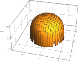
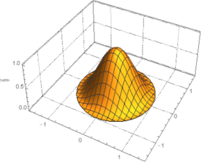
Figure 5.1. Plots of $\mathcal{B}_{\tau}(x)$ for (a) $\tau=\frac{1}{4}$ and (b) $\tau=\frac{5}{2}$.

Let $S^{1}:=\{(x_{1},x_{2})\in\mathbb{R}^{2}\;:\;x_{1}^{2}+x_{2}^{2}=1\}$ be the unit circle in $\mathbb{R}^{2}$. The function $\mathcal{B}_{\tau}$ is known to be Hölder continuous with exponent $\tau$ at every point in $S^{1}$. For illustration purpose, the plots of $\mathcal{B}_{\tau}(x)$ with $\tau=\frac{1}{4}$ and $\tau=\frac{5}{2}$ are displayed in Figure 5.1.

We now determine the Sobolev wavefront set of the function $\mathcal{B}_{\tau}$. The following result generalizes the result in [18] with $\tau=0$.

Proposition 22.

Let $\mathcal{B}_{\tau}$ be the function defined in (5.12) with $\tau>0$. Then

• For $(x_{1},x_{2})\in S^{1}$ and $s\neq\frac{x_{2}}{x_{1}}$ with $x_{1}\neq 0$, $\mathcal{SH}_{\psi}\mathcal{B}_{\tau}(a,s,t)$ decays rapidly as $a\to 0^{+}$.

• For $(x_{1},x_{2})\in S^{1}$ and $s=\frac{x_{2}}{x_{1}}$ with $x_{1}\neq 0$,

  (5.13) $$\mathcal{SH}_{\psi}\mathcal{B}_{\tau}(a,s,t)=\mathcal{O}(a^{\tau+\frac{3}{4}}),\qquad\mathcal{SH}^{(v)}_{\psi}\mathcal{B}_{\tau}(a,s,t)=\mathcal{O}(a^{\tau+\frac{3}{4}})\quad\mbox{as}\quad a\to 0^{+},$$

  where the above big $\mathcal{O}$ notation is defined in (1.13).

• For $(x_{1},x_{2})\not\in S^{1}$, $\mathcal{SH}_{\psi}\mathcal{B}_{\tau}(a,s,t)$ and $\mathcal{SH}^{(v)}_{\psi}\mathcal{B}_{\tau}(a,s,t)$ decay rapidly as $a\to 0^{+}$.

• For $(x_{1},x_{2})\in S^{1}$ and $m<\tau-\frac{1}{4}$, $((x_{1},x_{2}),\xi_{0})\not\in\operatorname{WF}_{m}(\mathcal{B}_{\tau})$ for all $\xi_{0}\in\mathbb{R}^{2}\backslash\{0\}$.

Proof.

Note that $\mathcal{B}_{\tau}$ is a bivariate radial function by $\mathcal{B}_{\tau}(x)=(1-|x|^{2})^{\tau}\chi_{[0,1]}(|x|)$ for all $x\in\mathbb{R}^{2}$. Through the polar coordinates, it is well known that its Fourier transform is given by

$$\widehat{\mathcal{B}_{\tau}}(\xi)=2\pi\int_{0}^{\infty}J_{0}(|\xi|t)\mathcal{B}_{\tau}(t)tdt=\frac{\Gamma(1+\tau)}{\pi^{\tau}}|\xi|^{-\tau-1}J_{\tau+1}(2\pi|\xi|),$$

where the Bessel function $J_{m}(\xi)$ of order $m>-\frac{1}{2}$ is defined to be

$$J_{m}(2\pi r)=\frac{r^{m}\pi^{m-\frac{1}{2}}}{\Gamma(m+\frac{1}{2})}\int_{-1}^{1}(1-t^{2})^{m-\frac{1}{2}}e^{2\pi irt}dt.$$

Note that $\widehat{\mathcal{B}_{\tau}}(\xi)=\mathcal{O}(|\xi|^{-\tau-\frac{3}{2}})$ as $|\xi|\to\infty$, because $J_{m}(2\pi r)\sim r^{-\frac{1}{2}}\left(e^{2\pi ir}+e^{-2\pi ir}\right)$ as $r\to\infty$.

(i) Using the polar coordinates, we have

$$\mathcal{SH}_{\psi} \mathcal{B}_{\tau}(a,s,t)=a^{\frac{3}{4}}\int_{\mathbb{R}^{2}}\widehat{\psi_{1}}(a\xi_{1})\widehat{\psi_{2}}\left(a^{-\frac{1}{2}}\left(\frac{\xi_{2}}{\xi_{1}}-s\right)\right)e^{2\pi i\xi\cdot t}\widehat{\mathcal{B}_{\tau}}(\xi)d\xi_{1}d\xi_{2}$$

$$=a^{-\frac{5}{4}}\int_{0}^{\infty}\int_{0}^{2\pi}\widehat{\psi_{1}}(\rho\ \cos\ \theta)\widehat{\psi_{2}}\left(a^{-\frac{1}{2}}\left(\tan\theta-s\right)\right)e^{2\pi i\rho(t_{1}\cos\theta+t_{2}\sin\theta)}\widehat{\mathcal{B}_{\tau}}\left(\frac{\rho}{a}\right)\rho d\theta d\rho$$

$$=a^{-\frac{5}{4}}\int_{0}^{\infty}I(a,s,t,\rho)\widehat{\mathcal{B}_{\tau}}\left(\frac{\rho}{a}\right)\ \rho\ d\rho,$$

where noting that $\operatorname{supp}(\widehat{\psi_{2}})\subseteq[-1,1]$, we define

$$I(a,s,t,\rho):=\int_{|\tan\theta-s|<\sqrt{a}}\widehat{\psi_{1}}(\rho\ \cos\ \theta)\widehat{\psi_{2}}\left(a^{-\frac{1}{2}}\left(\tan\theta-s\right)\right)e^{2\pi i\rho(t_{1}\cos\theta+t_{2}\sin\theta)}d\theta.$$

By [18, Lemma 4.9 and Proposition 4.7], we know that $I(a,s,t,\rho)$ is an oscillatory integral of the first kind that decays rapidly as $a\to 0^{+}$ for each $\rho>0$ when $s\neq x_{2}/x_{1}$. That is, for each $N\in\mathbb{N}$, there is a positive constant $C_{N}$ such that $\sup_{\rho\in(0,\infty)}\left|I(a,s,t,\rho)\right|\leq C_{N}a^{\frac{N}{2}}$. Hence the continuous shearlet transform $\mathcal{SH}_{\psi}\mathcal{B}_{\tau}(a,s,t)$ decays rapidly as $a\to 0^{+}$ when $s\neq x_{2}/x_{1}$.

(ii) Due to the rotation symmetry of $S^{1}$, it suffices to consider $x_{1}=1,x_{2}=0$ and hence $s=0$. Using the change of variable formula, one gets

$$\mathcal{SH}_{\psi}\mathcal{B}_{\tau}(a,0,(1,0))=a^{-\frac{3}{4}}\int_{0}^{\infty}\eta_{a}(\rho)\widehat{\mathcal{B}_{\tau}}\left(\frac{\rho}{a}\right)e^{2\pi i\frac{\rho}{a}}\ \rho\ d\rho$$

where

$$\eta_{a}(\rho) = \int_{-(1+a)^{-\frac{1}{2}}}^{(1+a)^{-\frac{1}{2}}}\widehat{\psi_{1}}(\rho\sqrt{1-au^{2}})\widehat{\psi_{2}}\left(\frac{u}{\sqrt{1-au^{2}}}\right)e^{2\pi i\frac{\rho}{a}(\sqrt{1-au^{2}}-1)}\frac{du}{\sqrt{1-au^{2}}}.$$

Note that $\widehat{\psi_{1}}$ is supported inside $[-2,-\frac{1}{2}]\cup[\frac{1}{2},2]$ and $\widehat{\psi_{2}}$ is supported inside $[-1,1]$. Now it is clear that the function $\eta_{a}(\rho)$ has compact support w.r.t. $\rho$. Hence,

$$\lim_{a\to 0^{+}}\eta_{a}(\rho)=\eta_{0}(\rho):=\int_{-1}^{1}\widehat{\psi_{1}}(\rho)\widehat{\psi_{2}}(u)e^{-\pi i\rho u^{2}}du=\widehat{\psi_{1}}(\rho)\int_{-1}^{1}\widehat{\psi_{2}}(u)e^{-\pi i\rho u^{2}}du.$$

The convergence of the integrand also holds for all derivatives w.r.t. $u$. Therefore, we can write

$$\mathcal{SH}_{\psi}\mathcal{B}_{\tau}(a,0,(1,0)) \sim a^{-\frac{3}{4}}\left(\int_{0}^{\infty}\left(\frac{a}{\rho}\right)^{\tau+\frac{3}{2}}\eta_{a}(\rho)e^{4\pi i\frac{\rho}{a}}\ \rho\ d\rho+\int_{0}^{\infty}\left(\frac{a}{\rho}\right)^{\tau+\frac{3}{2}}\eta_{a}(\rho)\ \rho\ d\rho\right)$$

$$= a^{\tau+\frac{3}{4}}\left(\widehat{F_{a,\tau}}\left(-\frac{2}{a}\right)+\int_{0}^{\infty}F_{a,\tau}(\rho)d\rho\right),$$

where $F_{a,\tau}(\rho)=\eta_{a}(\rho)\rho^{-\tau-\frac{1}{2}}$. By the uniform convergent properties of $\eta_{a}(\rho)$, $F_{a,\tau}(\rho)$ and all its derivatives, the function $\widehat{F_{a,\tau}}\left(-\frac{2}{a}\right)$ decays rapidly as $a\to 0^{+}$. The integral $\int_{0}^{\infty}F_{a,\tau}(\rho)d\rho$ converges to $\int_{0}^{\infty}\eta_{0}(\rho)\rho^{-\tau-\frac{1}{2}}d\rho$ as $a\to 0^{+}$. Since both $\widehat{\eta_{0}}$ and $\widehat{\psi_{1}}$ vanish on $[0,\infty)\backslash[\frac{1}{2},2]$, we have

$$\left|\int_{0}^{\infty}\eta_{0}(\rho)\rho^{-\tau-\frac{1}{2}}d\rho\right|= \left|\int_{0}^{\infty}\rho^{-\tau-1/2}\widehat{\psi}_{1}(\rho)\left(\int_{-1}^{1}\widehat{\psi}_{2}(u)e^{-i\pi\rho u^{2}}du\right)d\rho\right|$$

$$\leq \left|\int_{0}^{\infty}\rho^{-\tau-1/2}|\widehat{\psi}_{1}(\rho)|\int_{-1}^{1}|\widehat{\psi}_{2}(u)|dud\rho\right|$$

$$\leq \sqrt{2}\ \|\psi_{2}\|_{L^{2}}\int_{1/2}^{2}\rho^{-\tau-1/2}|\widehat{\psi}_{1}(\rho)|d\rho\leq\sqrt{3}\ 2^{\tau+1/2}\|\psi_{1}\|_{L^{2}}\|\psi_{2}\|_{L^{2}}<\infty.$$

This proves the first identity in (5.13) in item (ii). The second identity in (5.13) in item (ii) can be proved similarly.

(iii) follows from the localization property of shearlet (cf. [18, Proposition 3.4]).

(iv) The result follows easily from Theorem 3. ∎

Item (ii) in Proposition 22 only provides us an upper bound of shearlet coefficients. Following the argument of the lower bound estimates on shearlet coefficients in [10] for detecting singularities, by appropriately choosing $\psi_{1}$ and $\psi_{2}$, we now show that there exists a positive constant $c>0$ such that $|\mathcal{SH}_{\psi}\mathcal{B}_{\tau}(a,s,t)|\geq ca^{\tau+\frac{3}{4}}$ as $a\to 0^{+}$. To prove this claim, by the proof of (5.13) in item (ii), it suffices to prove that there exists $c>0$ such that $\left|\int_{0}^{\infty}\eta_{0}(\rho)\rho^{-\tau-\frac{1}{2}}d\rho\right|\geq c$. In addition to our assumption in (C1) and (C2) in Subsection 1.1, we now assume that $\widehat{\psi_{1}}(\xi)>0$ for all $\xi\in(-2,-\frac{1}{2})\cup(\frac{1}{2},2)$ and $\widehat{\psi_{2}}$ is supported inside $[-\frac{1}{2},\frac{1}{2}]$ such that $\widehat{\psi_{2}}(\xi)\geq 0$ for all $\xi\in[-\frac{1}{2},\frac{1}{2}]$. Then

$$\int_{-1}^{1}\widehat{\psi_{2}}(u)e^{-\pi i\rho u^{2}}du=\int_{-\frac{1}{2}}^{\frac{1}{2}}\widehat{\psi_{2}}(u)\cos(\pi\rho u^{2})du-i\int_{-\frac{1}{2}}^{\frac{1}{2}}\widehat{\psi_{2}}(u)\sin(\pi\rho u^{2})du=\widehat{\psi_{3}}(\rho)-i\widehat{\psi_{4}}(\rho),$$

where $\widehat{\psi_{3}}(\rho):=\int_{-1/2}^{1/2}\widehat{\psi_{2}}(u)\cos(\pi\rho u^{2})du$ and $\widehat{\psi_{4}}(\rho):=\int_{-1/2}^{1/2}\widehat{\psi_{2}}(u)\sin(\pi\rho u^{2})du$ for $\rho\geq 0$. Therefore, since all functions $\widehat{\psi_{1}},\ldots,\widehat{\psi_{4}}$ are real-valued functions, we conclude that

$$\left|\int_{0}^{\infty}\eta_{0}(\rho)\rho^{-\tau-\frac{1}{2}}d\rho\right|= \left|\int_{1/2}^{2}\rho^{-\tau-\frac{1}{2}}\widehat{\psi_{1}}(\rho)\widehat{\psi_{3}}(\rho)d\rho-i\int_{1/2}^{2}\rho^{-\tau-\frac{1}{2}}\widehat{\psi_{1}}(\rho)\widehat{\psi_{4}}(\rho)d\rho\right|$$

$$\geq \left|\int_{1/2}^{2}\rho^{-\tau-\frac{1}{2}}\widehat{\psi_{1}}(\rho)\widehat{\psi_{3}}(\rho)d\rho\right|,$$

For all $\rho\in[\frac{1}{2},2]$ and $|u|\leq 1/2$, we have $\cos(\pi\rho u^{2})\geq 0$ by $|\pi\rho u^{2}|<\pi/2$. Since we assumed that $\widehat{\psi_{2}}(\xi)\geq 0$ for $\xi\in[-1/2,1/2]$, we must have $\widehat{\psi_{3}}(\rho)\geq 0$ for all $\rho\in[\frac{1}{2},2]$. Note that $\widehat{\psi_{3}}$ cannot be identically zero on $[\frac{1}{2},2]$. Hence, we have

$$\left|\int_{0}^{\infty}\eta_{0}(\rho)\rho^{-\tau-\frac{1}{2}}d\rho\right|\geq\int_{1/2}^{2}\rho^{-\tau-\frac{1}{2}}\widehat{\psi_{1}}(\rho)\widehat{\psi_{3}}(\rho)d\rho=:c.$$

Because $\widehat{\psi_{1}}(\rho)>0$ and $\widehat{\psi_{3}}(\rho)\geq 0$ for all $\rho\in(\frac{1}{2},2)$, we must have $c>0$. This proves $|\mathcal{SH}_{\psi}\mathcal{B}_{\tau}(a,s,t)|\geq ca^{\tau+\frac{3}{4}}$ as $a\to 0^{+}$, which provides a lower bound for item (ii) in Proposition 22.

Acknowledgment: The authors would like to thank the reviewers for their valuable suggestions which improved the presentation of the paper.

References

- [1] H. Andrade-Loarca, G. Kutyniok, O. Öktem, and P. Petersen, Extraction of digital wavefront sets using applied harmonic analysis and deep neural networks, SIAM Journal on Imaging Science, 12 (2019), pp. 1936–1966.
- [2] C. Brouder, N. V. Dang, and F. Hélein, A smooth introduction to the wavefront set, Journal of Physics A: Mathematical and Theoretical, 47 (2014), p. 443001.
- [3] E. J. Candès and D. L. Donoho, New tight frames of curvelets and optimal representations of objects with piecewise singularities, Communications on Pure and Applied Mathematics, 57 (2004), pp. 219–266.
- [4] E. J. Candes and D. L. Donoho, Continuous curvelet transform: I. Resolution of the wavefront set, Applied and Computational Harmonic Analysis, 19 (2005), pp. 162–197.
- [5] M. V. De Hoop, K. Grochenig, and J. L. Romero, Exact and approximate expansions with pure gaussian wave packets, SIAM Journal on Mathematical Analysis, 46 (2014), pp. 2229–2253.
- [6] K. Guo, G. Kutyniok, and D. Labate, Sparse multidimensional representations using anisotropic dilation and shear operators, in Wavelets and splines: Athens, 2005, 189–201, Mod. Methods Math., Nashboro Press, TN.
- [7] K. Guo, D. Labate, W.-Q. Lim, G. Weiss, and E. Wilson, Wavelets with composite dilations and their mra properties, Applied and Computational Harmonic Analysis, 20 (2006), pp. 202–236.
- [8] K. Guo and D. Labate, Detection of singularities by discrete multiscale directional representations, The Journal of Geometric Analysis, 28 (2018), pp. 2102-2128.
- [9] K. Guo and D. Labate, Microlocal analysis of edge flatness through directional multiscale representations, Advances in Computational Mathematics, 43 (2017), pp. 295-318.
- [10] K. Guo and D. Labate, Characterization and analysis of edges using the continuous shearlet transform, SIAM on Imaging Sciences 2 (2009), pp. 959-986 .
- [11] B. Han, Vector cascade algorithms and refinable function vectors in Sobolev spaces, Journal of Approximation Theory, 124 (2003), pp. 44–88.
- [12] B. Han, Framelets and wavelets: Algorithms, analysis, and applications. Applied and Numerical Harmonic Analysis. Birkhäuser/Springer, Cham, 2017. xxxiii + 724 pp.
- [13] L. Hörmander, The analysis of linear partial differential operators, Springer, Berlin, 1983.
- [14] L. Hörmander, Lectures on nonlinear hyperbolic differential equations, vol. 26, Springer Science & Business Media, 1997.
- [15] S. Jaffard, Pointwise smoothness, two-microlocalization and wavelet coefficients, Publicacions Matematiques, 35 (1991), pp. 155–168.
- [16] S. Jaffard and Y. Meyer, Wavelet methods for pointwise regularity and local oscillations of functions. Memoirs of the American Mathematical Society, 123 (1996), x+110 pp.
- [17] K. M. Kolwankar and J. L. Véhel, A time domain characterization of the fine local regularity of functions, Journal of Fourier Analysis and Applications, 8 (2002), pp. 319–334.
- [18] G. Kutyniok and D. Labate, Resolution of the wavefront set using continuous shearlets, Transactions of the American Mathematical Society, 361 (2009), pp. 2719–2754.
- [19] G. Kutyniok and P. Petersen, Classification of edges using compactly supported shearlets, Applied and Computational Harmonic Analysis 42 (2017) pp. 245-293.
- [20] D. Labate, W.-Q. Lim, G. Kutyniok, and G. Weiss, Sparse multidimensional representation using shearlets, in Wavelets XI, vol. 5914, International Society for Optics and Photonics, 2005, p. 59140U.
- [21] P. Lakhonchai, J. Sampo, and S. Sumetkijakan, Shearlet transforms and directional regularities, International Journal of Wavelets, Multiresolution and Information Processing, 8 (2010), pp. 743–771.
- [22] K. Nualtong and S. Sumetkijakan, Analysis of hölder regularity by wavelet-like transforms with parabolic scaling, Thai Journal of Mathematics, 3 (2005), pp. 275–283.
- [23] B. E. Petersen, Introduction to the Fourier transform & pseudo-differential operators, Pitman Advanced Publishing Program, 1983.
- [24] J. Sampo and S. Sumetkijakan, Estimations of hölder regularities and direction of singularity by hart smith and curvelet transforms, Journal of Fourier Analysis and Applications, 15 (2009), pp. 58–79.
- [25] S. Seuret and J. L. Véhel, A time domain characterization of 2-microlocal spaces, Journal of Fourier Analysis and Applications, 9 (2003), pp. 473–495.
- [26] S. Seuret and J. L. Véhel, A time domain characterization of 2-microlocal spaces, Technical Report RR-4545, INRIA, (2002).