The Asymptotic Iteration Method Revisited

Abstract

The Asymptotic Iteration Method (AIM) is a technique for solving analytically and approximately the linear second-order differential equation, especially the eigenvalue problems that frequently appear in theoretical and mathematical physics. The analysis and mathematical justifications of the success and failure of the asymptotic iteration method are detailed in this work. A theorem explaining why the asymptotic iteration method works for the eigenvalue problem is presented. As a byproduct, a new procedure to generate unlimited classes of exactly solvable differential equations is also introduced.

1 Introduction

Since the first publication Cif:Hal:Saa of the Asymptotic Iteration Method (AIM), it has enjoyed great success in many areas of physics, among them we refer the reader to the references cho:cor:dou ; cho:dou:nay ; boz:bon ; Ci:Ha:Sa ; Dm:Mm:Jk ; Gk:Ob:Ib . Given the differential equation

$$y^{\prime\prime}(x)=\lambda_{0}(x)y^{\prime}(x)+s_{0}(x)y(x),$$ (1)

where $\lambda_{0}(x)$ and $s_{0}(x)$ are $C^{\infty}$ functions. AIM uses the invariant structure of the right-hand side of (1) under further differentiation. Indeed, the $n-1$ and $n$ differentiation of Eq.(1) gives, respectively,

$$\begin{gathered}y^{(n+1)}(x)=\lambda_{n-1}(x)y^{\prime}(x)+s_{n-1}(x)y(x),\\ y^{(n+2)}(x)=\lambda_{n}(x)y^{\prime}(x)+s_{n}(x)y(x),\end{gathered}$$ (2)

where the AIM sequences $\lambda_{n}(x)$ and $s_{n}(x)$, $n=1,2,\dots$ are, recursively, evaluated using the relations

$$\begin{gathered}\lambda_{n}(x)=\lambda_{n-1}^{\prime}(x)+s_{n-1}(x)+\lambda_{0}(x)\lambda_{n-1}(x)\\ s_{n}(x)=s_{n-1}^{\prime}(x)+s_{0}(x)\lambda_{n-1}(x).\end{gathered}$$ (3)

When (1) has a polynomial solution of degree $n$, Ciftci, Hall, and Saad Cif:Hal:Saa proved that the general solution is given by

$$y(x) =C_{1}\exp\left(-\int^{x}\alpha_{n}(t)dt\right)+C_{2}\exp\left(-\int^{x}\alpha_{n}(t)dt\right)\int^{x}\exp\left(\int^{t}[\lambda_{0}(u)+2\,\alpha_{n}(u)]du\right)dt,$$ (4)

where

$$\alpha_{n}(x)=s_{n-1}(x)/\lambda_{n-1}(x)$$ (5)

and $\{\lambda_{k}(x)\}$ and $\{s_{k}(x)\}$ satisfy the termination condition

$$\delta_{n}(x)=\lambda_{n}(x)s_{n-1}(x)-\lambda_{n-1}(x)s_{n}(x)=0,\qquad n=1,2,\dots.$$ (6)

Using (2), it easily follows that

$$\lambda_{n}(x)y^{(n+1)}(x)-\lambda_{n-1}(x)y^{(n+2)}(x)=\delta_{n}(x)y(x)$$ (7)

whence if $y(x)$, the solution of (1), is a polynomial of degree at most $n$ then $\delta_{n}(x)\equiv 0$. On the other hand, if $\delta_{n}(x)\equiv 0$, a particular solution of the differential equation (1) is given by $y(x)=\exp\left(-\int^{x}\alpha_{n}(t)dt\right)$. Therefore, using (2),

$$y^{(n+1)}(x)=\left[\lambda_{n}(x)s_{n-1}(x)-\lambda_{n-1}(x)s_{n}(x)\right]y(x)=0,$$ (8)

and consequently $y(x)$ is a polynomial of degree at most $n$. It is not difficult Saa:Hal:Cif to also verify that if $\delta_{n}(x)\equiv 0$, then $\delta_{m}(x)=0$ for all $m\geq n$.

Part of AIM’s success is due to the inherent simplicity of its iterative process governed by the termination condition (6) as well for its ability to obtain not only explicit solutions but possibly accurate approximations if the solution is not a polynomial.

Until now, there is no rigorous justification given for the validity of the answers when equation (1) does not have a polynomial solution. In particular the treatment of the constant-coefficient differential equations in Cif:Hal:Saa is not only not rigorous but misses an important feature of AIM, which we will elaborate on in this work. There were also other cases where AIM failed as pointed out in the works of Barakat Bara , P. Amore and F. M. Fernández F2006 , and Fernandez F2004 . Sometimes a transformation of the problem makes it amenable for AIM to be applied. What is really mysterious is that AIM appears to give correct answers even in certain cases when $\delta_{n}(x)\not\equiv 0$ for any finite $n$. There are cases where AIM did not work, see F2004 and Bara but, besides the cases of polynomial solutions, no explanation was given as to when AIM works or the iterative procedure in the AIM does not converge. The present paper is a step towards understanding these issues. This is a first step towards a rigorous theory explaining how and why AIM works. This is important since AIM is an especially powerful tool when it comes to numerical computations.

The present work provides not just the mathematical justification that accounts for the success of AIM and why the iterative procedure in the AIM does converge, but we also illustrate cases of failure of the AIM procedure in fairly simple examples. Luckily the algorithm which implements AIM predicts the cases of failure. The present work also provides a technique to generate a chain of a solvable class of differential equations that approximate the exact solution to a given second-order linear differential equation. Theorems 2.1 (see below) is a device which iteratively produces new solvable differential equations. Theorem 2.1 proves that AIM a robust and reliable technique for solving the differential equations (1). We start, in the next section, by explaining why AIM gives the correct solutions for a certain class of constant-coefficient differential equations although, for a fixed $n$, the termination condition (6) cannot vanish identically. Starting from an equation of the form (1), we give a chain of differential equations with two explicitly defined solutions. The main results of the present work are shown in Sections 2, 3, and 4. We believe that the case of constant coefficients has all the characteristics of the general case. In the sense that AIM carries the attributes of success and failure as in the general case that depends on the nature of the differential equation coefficients, so we include in Section 3 a complete treatment of the case of constant coefficients as an illustration of the AIM technique. We show that AIM works if and only if the two roots of the characteristic equation have different moduli unless they are equal. We explicitly give examples of linear second-order differential equations with real constant coefficients where the AIM technique fails. Still, luckily, we indicate that the numerics predicts the failure of the method. Section 4 contains all the numerical examples where AIM is implemented and correctly predicts the cases of success or failure. Section 5 treats an example where $\lambda_{0}(x)$ is a linear polynomial. This treatment leads to generate a chain of linear second-order differential equations with rational coefficients and explicit bases of solutions. In Section 6, we give an elementary, but practical, treatment of the classical anharmonic oscillator potential $V(x)=x^{2}+Ax^{4}$, $A\geq 0$. Interestingly, this simple approach gives the eigenvalues accurate to fifty decimals. In Section 7, a conclusion is provided that summarizes the results presented in this work.

2 Main Results

In this section, we state the main results of the present work.

Theorem 2.1.

Let

$$\begin{gathered}y_{n}(x)=\exp\left(-\int^{x}\alpha_{n}(t)dt\right),\\ z_{n}(x)=\exp\left(-\int^{x}\alpha_{n}(t)dt\right)\int^{x}\exp\left(\int^{t}[\lambda_{0}(u)+2\alpha_{n}(u)du\right)dt.\end{gathered}$$ (9)

Then $y_{n}(x)$ and $z_{n}(x)$ are linear independent solutions of the differential equation

$$y^{\prime\prime}(x)-\lambda_{0}(x)y^{\prime}(x) -s_{0}(x)y(x)=\frac{\lambda_{n}(x)s_{n-1}(x)-s_{n}(x)\lambda_{n-1}(x)}{\lambda_{n-1}^{2}(x)}\;y(x).$$ (10)

Proof: It is a calculus exercise to use $y_{n}^{\prime}(x)=-y_{n}(x)s_{n-1}(x)/\lambda_{n-1}(x)$ to show that $y_{n}(x)$ satisfies (10). To find a second solution of (10) write $y(x)=y_{n}(x)u_{n}(x)$ and use the variation of parameters to find $u_{n}(x)$ and the solution $y_{n}(x)u_{n}(x)$ turns out to be $z_{n}(x)$. It can be easily verified that the Wronskian of $y_{n}(x)$ and $z_{n}(x)$ is not zero. $\square$ Theorem 2.1 explains the gist of AIM. Indeed when $\delta_{n}(x)\equiv 0$ then the perturbed differential equation (10) reduces to (1), so $y_{n}(x)$ and $z_{n}(x)$ are two linear independent solutions of the original equation (1). In general (10) is a perturbation of (1), so what is needed is a rigorous theory that shows that for certain class of functions $\lambda_{0}(x)$ and $s_{0}(x)$ the coefficient of $y(x)$ on the right-hand side of (10) tends to zero as $n\to\infty$. One also needs to show that when $\delta_{n}(x)/\lambda_{0}(x)^{2}\to 0$ the solution of equation (10) converge to solution of the original equation (1). We shall explore this fact through a number of examples in the next section.

We note that if $\lambda_{0}(x)$ and $s_{0}(x)$ are rational functions then $\lambda_{n}(x)$ and $s_{n}(x)$ are also rational functions, hence $\alpha_{n}(x)$ is a rational function. If we further assume that the poles of $\alpha_{n}(x)$ are all simple then $y_{n}(x)$, up to a constant multiple, takes the form

$$y_{n}(x)=e^{p(x)}\prod_{j}(1-x/x_{j})^{a_{j}},$$ (11)

where $p(x)$ is a polynomial. On the other hand the function $z_{n}$ involves an indefinite integral of a function of the above form.

We note that

$$\begin{gathered}\frac{\lambda_{n}(x)s_{n-1}(x)-s_{n}(x)\lambda_{n-1}(x)}{\lambda_{n-1}^{2}(x)}+s_{0}(x)=-\dfrac{d}{dx}\left(\dfrac{s_{n-1}(x)}{\lambda_{n-1}(x)}\right)+\left(\dfrac{s_{n-1}(x)}{\lambda_{n-1}(x)}\right)^{2}+\lambda_{0}\left(\dfrac{s_{n-1}(x)}{\lambda_{n-1}(x)}\right).\end{gathered}$$ (12)

This allows us to write a different form of the differential equation (10).

3 Constant Coefficients differential equations

In the case of constant coefficients, the AIM sequences (3) reduces to

$$\begin{gathered}\lambda_{n}=\lambda_{n-1}\lambda_{0}+s_{n-1},\quad s_{n}=\lambda_{n-1}s_{0},\quad n>0.\end{gathered}$$ (14)

Therefore, $\lambda_{n}$ and $s_{n}$ satisfy the recurrence relation

$$\nu_{n+1}=\lambda_{0}\,\nu_{n}+s_{0}\,\nu_{n-1},$$ (15)

where $\lambda_{0}$ and $s_{0}$ are constants. The characteristic equation is $r^{2}-\lambda_{0}r-s_{0}=0$ with roots

$$r_{1},r_{2}=\dfrac{\lambda_{0}}{2}\pm\sqrt{s_{0}+\dfrac{\lambda_{0}^{2}}{4}}.$$ (16)

We may assume $|r_{2}|\leq|r_{1}|$. It is clear that $r_{1}+r_{2}=\lambda_{0}$ and $r_{1}\,r_{2}=-s_{0}.$

3.1 Two roots with distinct moduli

If $s_{0}+\lambda_{0}^{2}/4\neq 0$ then

$$\lambda_{n}=Ar_{1}^{n}+(\lambda_{0}-A)r_{2}^{n},\quad s_{n}=Br_{1}^{n}+(s_{0}-B)r_{2}^{n},$$ (17)

where $A$ and $B$ are constants, and $\lambda_{1}=\lambda_{0}^{2}+s_{0},s_{1}=\lambda_{0}s_{0}$. Also note that $r_{1}+r_{2}=\lambda_{0},r_{1}r_{2}=-s_{0}$.

$$\begin{gathered}A(r_{1}-r_{2})=\lambda_{1}-\lambda_{0}r_{2}=\lambda_{0}^{2}+s_{0}-\lambda_{0}r_{2}=\lambda_{0}r_{1}+s_{0}=r_{1}^{2},\\ B(r_{1}-r_{2})=s_{1}-s_{0}=\lambda_{0}s_{0}-s_{0}r_{2}=s_{0}r_{1}.\end{gathered}$$ (20)

Therefore the ratio $\alpha_{n+1}=s_{n}/\lambda_{n}$ has the form

$$\alpha_{n+1}=\frac{Br_{1}^{n}+(s_{0}-B)r_{2}^{n}}{Ar_{1}^{n}+(\lambda_{0}-A)r_{2}^{n}}.$$ (21)

In this case $|r_{1}|>|r_{2}|$. Thus, for large $n$, we conclude that

$$\alpha_{n}\approx B/A=s_{0}/r_{1}=-r_{2}.$$ (22)

while

$$\lambda_{0}+\alpha_{n}\approx\lambda_{0}+B/A=r_{1}+r_{2}+s_{0}/r_{1}=r_{1},$$ (23)

Equation (4) indicates that one solution is $\exp(-\alpha_{n}x)=\exp(r_{2}\,x)$ while the second linearly independent solution is $\exp((\lambda_{0}+\alpha_{n})x)=\exp(r_{1}\,x)$, as expected by the classical theory of differential equations with constant coefficients. It must be noted that in the present case the perturbation term in (10) decays exponentially as $n\to\infty$. Indeed

$$\frac{\lambda_{n}(x)s_{n-1}(x)-s_{n}(x)\lambda_{n-1}(x)}{\lambda_{n-1}^{2}(x)}=\mathcal{O}(({r_{2}}/{r_{1}})^{n}),$$

is true. In general AIM approach fails when $|r_{1}|=|r_{2}|$, and $r_{1}\neq r_{2}$. This easily follows from (21). The good news is that the AIM algorithm sees this very early on and in Section 5 we will illustrate this by an example.

3.2 Double root

In the case of $s_{0}+\lambda_{0}^{2}/4=0$, the solution of the difference equation (15) assumes the form, for $r_{1}=r_{2}=r=\lambda_{0}/2$. Thus $\lambda_{n}$ and $s_{n}$ have the forms

$$\lambda_{n}=r^{n}(\lambda_{0}+An),\qquad s_{n}=r^{n}(s_{0}+Bn).$$ (24)

with the initial conditions $\lambda_{1}=\lambda_{0}^{2}+s_{0},\quad s_{1}=s_{0}\lambda_{0}.$ From here it follows that $A=r,B=-r^{2}$ The solution (24) now reads

$$\lambda_{n}=r^{n}(n+2),\qquad s_{n}=-r^{n+2}(n+1).$$ (25)

Thus, for large $n$,

$$\alpha_{n}=s_{n-1}/\lambda_{n-1}\approx-r.$$ (26)

Now the general solution reads

$$\begin{gathered}y(x)=C_{1}e^{rx}+C_{2}\,x\,e^{rx},\end{gathered}$$ (28)

again as expected by the general theory of differential equations. In the present case the perturbation term in Eq.(10) is given by

$$\frac{\lambda_{n}(x)s_{n-1}(x)-s_{n}(x)\lambda_{n-1}(x)}{\lambda_{n-1}^{2}(x)}=\mathcal{O}(1/n^{2}),$$

confirming that the perturbation term tends to zero.

We note that matrix form of (3) is

$$\begin{gathered}\left(\begin{matrix}\lambda_{n}(x)\\ s_{n}(x)\end{matrix}\right)=\left[\frac{d}{dx}+\left(\begin{matrix}\lambda_{0}(x)&1\\ s_{0}(x)&0\end{matrix}\right)\right]\left(\begin{matrix}\lambda_{n-1}(x)\\ s_{n-1}(x)\end{matrix}\right).\end{gathered}$$ (30)

Therefore the solution is

$$\begin{gathered}\left(\begin{matrix}\lambda_{n}(x)\\ s_{n}(x)\end{matrix}\right)=\left[\frac{d}{dx}+\left(\begin{matrix}\lambda_{0}(x)&1\\ s_{0}(x)&0\end{matrix}\right)\right]^{n}\left(\begin{matrix}\lambda_{0}(x)\\ s_{0}(x)\end{matrix}\right).\end{gathered}$$ (32)

This raises the issue of finding an expansion formula for

$$\left[\frac{d}{dx}+\left(\begin{matrix}\lambda_{0}(x)&1\\ s_{0}(x)&0\end{matrix}\right)\right]^{n}f(x)$$ (33)

In the scalar case expansions of the above type are known. For example Burchnall Bur proved that

$$\left(\frac{d}{dx}-2x\right)^{m}f(x)=\sum_{k=0}^{m}(-1)^{n-k}{m\choose k}H_{m-k}(x)f^{(k)}(x),$$ (34)

where $H_{m-k}(x)$ is Hermite polynomial. Several related expansions involving Laguerre and Jacobi polynomials, as well as their $q$-analogues, have been established recently in Ism:Koe:Rom and Ism:Koe:Rom2 . We now show how this applies to the case of linear second order differential equations with constant coefficients It is easy to see that

$$\left(\begin{matrix}\lambda_{0}&1\\ s_{0}&0\end{matrix}\right)=CDC^{-1},\quad C=\left(\begin{matrix}r_{1}&r_{2}\\ s_{0}&s_{0}\end{matrix}\right),D=\left(\begin{matrix}r_{1}&0\\ 0&r_{2}\end{matrix}\right).$$ (35)

Therefore

$$\begin{gathered}\left[\frac{d}{dx}+\left(\begin{matrix}\lambda_{0}(x)&1\\ s_{0}(x)&0\end{matrix}\right)\right]^{n}f(x)=C\left(\begin{matrix}\exp(-xr_{1})&0\\ 0&\exp(-xr_{2})\end{matrix}\right)\frac{d^{n}}{dx^{n}}\left[\left(\begin{matrix}\exp(xr_{1})&0\\ 0&\exp(xr_{2})\end{matrix}\right)C^{-1}f(x)\right].\end{gathered}$$ (37)

Motivated by Burchnall’s formula (34) we formulate the following problem. Problem: Let $\lambda_{0}(x)$ and $s_{0}(x)$ be $n$ times continuously differentiable functions. Is there an explicit formula for

$$\left[\frac{d}{dx}+\left(\begin{matrix}\lambda_{0}(x)&1\\ s_{0}(x)&0\end{matrix}\right)\right]^{n}\left(\begin{matrix}f_{1}(x)\\ f_{2}(x)\end{matrix}\right).$$ (38)

4 Applications: Constant coefficient differential equations

In the original publication of AIM Cif:Hal:Saa , the authors explore its application in solving the constant coefficient differential equations when the roots of the associated characteristic equation are real distinct. No attempt for the other possible cases was ever discussed. This may have gave a misleading impression that AIM always applicable for this class of equations. The examination for AIM convergence, Section 3, shows a drawback in AIM usage in handling the constant coefficient differential equations when the associated characteristic equations has ‘equal’ moduli complex roots. Although, this is not a small class of equations, the information extracted from AIM usage are not all lost, for the oscillation behavior of $\alpha_{n}$ serve as an indicator for the peculiar form of the complex roots. Consider, for example, the differential equation

$$y^{\prime\prime}-2\cos(\pi/8)y^{\prime}+\,y=0,$$ (39)

The evaluation of $\alpha_{n}=s_{n-1}/\lambda_{n-1},$ and $\delta_{n}(x)/\lambda_{n-1}^{2}$ for $n=1,2,\dots,150$ are illustrated in the figure 1.

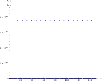
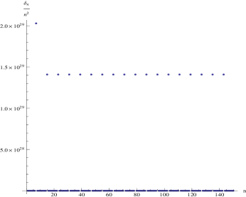
Figure 1: The discrete points along the horizontal line and the $n$-axis illustrate the oscillation behaviour of $\alpha_{n}$ and $\delta_{n}/\lambda_{n-1}$ for $n=1,2,\dots,150$ produced by AIM in handling the differential equation (39).

This oscillation behavior predict that the roots of the characteristic equation $r^{2}-2\cos(\pi/8)r+\,1=0$, namely, $r_{1}=\cos(\pi/8)+i\sin(\pi/8)$ and $r_{2}=\cos(\pi/8)-i\sin(\pi/8)$ have equal moduli. We illustrate another strange behaviour produced by AIM numerical evaluation by the following example. Consider the differential equation

$$y^{\prime\prime}-2\cos(\pi/4)y^{\prime}+\,y=0,$$ (40)

The evaluation of $\alpha_{n}$ and $\delta_{n}(x)/\lambda_{n-1}$ using AIM sequences are displayed in Figure (2).

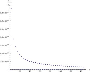
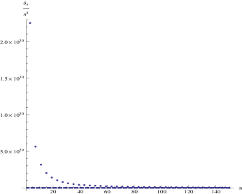
Figure 2: The discrete points along the exponential-type curve and the $n$-axis illustrate the strange behaviour of $\alpha_{n}$ and $\delta_{n}/\lambda_{n-1}$ for $n=1,2,\dots,150$ produced by AIM in handling the differential equation (40).

Again such response of AIM is confirmed by the modulus of the complex roots of the characteristic equation, namely $r_{1}=(1-i)/\sqrt{2}$ and $r_{2}=(1+i)/\sqrt{2}$.

Let us now consider the general case when $\lambda_{0}$ and $s_{0}$ are real and $|r_{1}|=|r_{2}|=r$, say. Let $r_{1},r_{2}=re^{i\theta},re^{-i\theta}$. In this case (21) gives

$$\alpha_{n+1}=\frac{2\,i\,B\,\sin(n\,\theta)+s_{0}\,e^{-in\theta}}{2\,i\,A\,\sin(n\,\theta)+\lambda_{0}\,e^{-in\theta}}.$$

If $\theta$ is a rational number $\in(0,\pi/2)$ we can choose $n$ to be an arithmetic progression which makes $\sin(n\theta)=0$ while $r_{1}-r_{2}=2ir\sin\theta\neq 0$, hence $A$ and $B$ are well defined. On such a sequence $\alpha_{n+1}$ takes the constant value $s_{0}/\lambda_{0}$, which gives the wrong answer. The point we are trying to make is that in such cases AIM fails and looking at subsequences does not help.

Another class that was overlooked in Cif:Hal:Saa is the linear differential equations with complex coefficients. AIM gives the exact solutions as long as the roots of the associated characteristic equation have different norms. A class of such equations is given by

$$y^{\prime\prime}-a\,i\,y^{\prime}-b\,(b+a\,i)\,y=0,\qquad i=\sqrt{-1},\quad a,b\in\mathbb{R}$$ (41)

Take $a=b=2$, Eq.(41) then reads

$$y^{\prime\prime}(x)-2\,i\,y^{\prime}(x)-(4+4\,i)\,y(x)=0.$$ (42)

AIM tends to the exact solutions $\{e^{2x},e^{(2+2i)x}\}$ as $n$ gets larger and larger as the figure (3) shows.

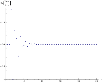
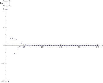
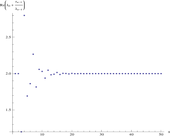
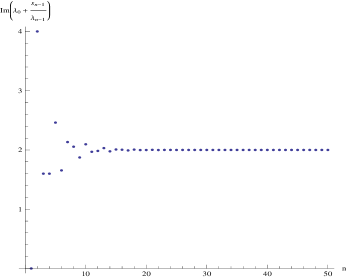
Figure 3: The convergence of $\alpha_{n}$ and $\lambda_{0}+\alpha_{n}$ for $n=1,2,\dots,50$, produced by AIM, to exact solutions of the equation (42).

5 Applications: Rational coefficient differential equations

As an example, we establish classes of exact-solvable differential equations initiated with rational coefficients in the form

$$y^{\prime\prime}(x)-\mu\,x\,y^{\prime}(x)+\eta\,y(x)=0.$$ (43)

Starting with $\lambda_{0}=\mu\,x$ and $s_{0}=-\eta,$ the first-iteration using Theorem 2.1 implies

$$y_{1}^{\prime\prime}(x)-\mu\,x\,y_{1}^{\prime}(x)+\eta\,y_{1}(x)=\frac{\eta(\eta-\mu)}{\mu^{2}x^{2}}\,y_{1}(x)~{}\mbox{with}~{}y_{1}(x)=x^{\eta/\mu}.$$ (44)

This differential equation generate, for example, infinite classes of exactly solvable differential equations

$$x^{2}u^{\prime\prime}(x)-\mu\,x^{3}\,u^{\prime}(x)+m\left(\mu\,x^{2}-m+1\right)\,u(x)=0\quad\mbox{with}\quad u(x)=x^{m},~{}m=0,\pm 1,\pm 2,\dots,$$ (45)

and, with the replacement $x$ with $1/x$,

$$x^{4}\,v^{\prime\prime}(x)+x\left(2\,x^{2}+\mu\right)\,v^{\prime}(x)+m\left(\mu-(m-1)\,{x^{2}}\right)\,v(x)=0~{}\mbox{with}~{}~{}v(x)={x^{-m}},$$ (46)

for $m=0,\pm 1,\pm 2,\dots$. The second iteration, using Theorem 2.1, yields

$$y_{2}^{\prime\prime}(x)-\mu\,x\,y_{2}^{\prime}(x)+\eta\,y_{2}(x)=\frac{\eta(\eta-\mu)(\eta-2\mu)}{\left(\mu-\eta+\mu^{2}x^{2}\right)^{2}}\,y_{2}(x)\quad\mbox{with}\quad y_{2}(x)=\left(\eta-\mu-\mu^{2}x^{2}\right)^{{\eta}/({2\mu})}.$$ (47)

This differential equation also generate infinite classes of exactly solvable differential equations, for example,

$$y_{2}^{\prime\prime}(x)-\mu\,x\,y_{2}^{\prime}(x)+2\,m\,\mu\,\left(1-\frac{2(m-1)(2m-1)}{\left(1-2m+\mu x^{2}\right)^{2}}\right)y_{2}(x)=0,$$

where

$$y_{2}(x)=(1-2m+\mu\,x^{2})^{m},\quad m=0,1,2,\dots.$$

The third iteration, using Theorem 2.1, yields

$$y_{3}^{\prime\prime}(x)-\mu\,x\,y_{3}^{\prime}(x)+\eta\,y_{3}(x)=\frac{\eta(\eta-\mu)(\eta-2\mu)(\eta-3\mu)}{\mu^{2}x^{2}\left(3\mu-2\eta+\mu^{2}x^{2}\right)^{2}}\,y_{3}(x)$$ (48)

with exact solution

$$y_{3}(x)=x^{{\eta(\eta-2\mu)}/({(2\eta-3\mu)\mu})}\left(2\eta-3\mu-\mu^{2}x^{2}\right)^{{\eta(\eta-\mu)}/{(2\mu({2\eta-3\mu})})}$$ (49)

The fourth iteration, using Theorem 2.1, yields

$$y_{4}^{\prime\prime}(x)-\mu\,x\,y_{4}^{\prime}(x)+\eta\,y_{4}(x)=\frac{\eta(\eta-\mu)(\eta-2\mu)(\eta-3\mu)(\eta-4\mu)}{(\eta-3\mu)(\eta-\mu)-3(\eta-2\mu)\mu^{2}x^{2}+\mu^{4}x^{4}}\,y_{4}(x)$$ (50)

with exact solution given by

$$y_{4}(x) =\left((\eta-3\mu)(\eta-\mu)-3(\eta-2\mu)\mu^{2}x^{2}+\mu^{4}x^{4}\right)^{{\eta}/({4\mu})}$$

$$\times\left(\sqrt{5\eta^{2}-20\eta\mu+24\mu^{2}}+3\eta-2\mu\left(3+\mu x^{2}\right)\right)^{-\tfrac{\eta(\eta-4\mu)}{4\mu\sqrt{5\eta^{2}-20\eta\mu+24\mu^{2}}}}$$

$$\times\left({\sqrt{5\eta^{2}-20\eta\mu+24\mu^{2}}}-3\eta+2\mu\left(3+\mu x^{2}\right)\right)^{\tfrac{\eta(\eta-4\mu)}{4\mu\sqrt{5\eta^{2}-20\eta\mu+24\mu^{2}}}}$$ (51)

The fifth iteration, using Theorem 2.1, yields

$$y_{5}^{\prime\prime}(x)-\mu\,x\,y_{5}^{\prime}(x) +\eta\,y_{5}(x)=\dfrac{\eta(\eta-\mu)(\eta-2\mu)(\eta-3\mu)(\eta-4\mu)(\eta-5\mu)}{\mu^{2}x^{2}\left(3\left(\eta^{2}-5\eta\mu+5\mu^{2}\right)-2(2\eta-5\mu)\mu^{2}x^{2}+\mu^{4}x^{4}\right)^{2}}\,y_{5}(x)$$ (52)

with exact solution given by

$$y_{5}(x) =x^{\tfrac{\eta(\eta-4\mu)(\eta-2\mu)}{3\mu\left(\eta^{2}-5\eta\mu+5\mu^{2}\right)}}$$

$$\times\left(5\mu-2\eta+\mu^{2}x^{2}-\sqrt{\eta^{2}-5\eta\mu+10\mu^{2}}\right)^{\tfrac{\eta(\eta-\mu)\left((2\eta-7\mu)\sqrt{\eta^{2}-5\eta\mu+10\mu^{2}}-(\eta-5\mu)(\eta-4\mu)\right)}{12\mu\left(\eta^{2}-5\eta\mu+5\mu^{2}\right)\sqrt{\eta^{2}-5\eta\mu+10\mu^{2}}}}$$

$$\times\left(5\mu-2\eta+\mu^{2}x^{2}+\sqrt{\eta^{2}-5\eta\mu+10\mu^{2}}\right)^{\tfrac{\eta(\eta-\mu)\left((\eta-5\mu)(\eta-4\mu)+(2\eta-7\mu)\sqrt{\eta^{2}-5\eta\mu+10\mu^{2}}\right)}{12\mu\left(\eta^{2}-5\eta\mu+5\mu^{2}\right)\sqrt{\eta^{2}-5\eta\mu+10\mu^{2}}}}$$ (53)

Clearly, for $\eta=m\mu$, $m=0,1,2,\dots$, the general solutions of the generalized Hermite equation

$$y_{m}^{\prime\prime}(x)-\mu\,x\,y_{m}^{\prime}(x)+m\,\mu\,y_{m}(x)=0,\quad m=0,1,2,\dots.$$ (54)

reads

$$y_{0}(x) =1,\quad y_{1}(x)=x,\quad y_{2}(x)=\mu\,x^{2}-1,\quad y_{3}(x)=x(\mu x^{2}-3),~{}\dots$$ (55)

with a general expression given in terms of the Hermite polynomials as

$$y_{m}:=H_{m}\left(\sqrt{\dfrac{\mu}{2}}\,x\right),$$ (56)

up to a constant.

6 One-dimensional anharmonic oscillator potentials

We consider a class of one-dimensional anharmonic oscillator potentials discussed by Ciftci, Hall and Saad in their original work on AIM that reflects on its powerful computaional aspect:

$$V(x)=x^{2}+A\,x^{4},\quad A\geq 0,\quad x\in(-\infty,\infty).$$ (57)

Schrödinger’s equation for $V(x)$ takes the form (in the units $m=2\hbar=1$)

$$-\dfrac{d^{2}\psi}{dx^{2}}+\left(x^{2}+A\,x^{4}\right)\psi=E\psi,\quad\int_{-\infty}^{\infty}|\psi(x)|dx<\infty.$$ (58)

Using the asymptotic solution near $A=0,$ a general solution of (58) take the form

$$\psi(x)=e^{-x^{2}/2}f(x),$$ (59)

which up on substituting into (58) gives the differential equation of $f(x)$ as

$$\dfrac{d^{2}f}{dx^{2}}-2\,x\,f^{\prime}(x)-\left(1-E+A\,x^{4}\right)\,f=0.$$ (60)

Theorem 2.1 gives, as a first approximation of equation (60),

$$f^{\prime\prime}(x)-2\,x\,f^{\prime}(x) -\left(1-E+A\,x^{4}\right)\,f(x)=\frac{(E-3)(E-1)-2A(E+2)\,x^{4}+A^{2}\,x^{8}}{4\,x^{2}}f(x),$$ (61)

with exact solution given by

$$f(x)=x^{(E-1)/2}e^{-A\,x^{4}/8}.$$ (62)

The right-hand side of (61) confirm that the termination condition $\delta_{1}(x)=0$ depends explicitly on the variable $x\neq 0$ and the unknown $E$ for the given parameter $A$. Further, for the initial starting of $x_{0}$, we should start sighlty away from $x_{0}=0$ because $\delta_{1}(x)=0$ will yields $E=1$ or $E=3$. Thus, for a good initial starting of $x_{0}$ is $x_{0}=0.0001$. As a second approximation, Theorem 2.1 gives

$$f^{\prime\prime}(x)-2\,x\,f^{\prime}(x) -\left(1-E+A\,x^{4}\right)\,f(x)=\tfrac{(E-5)(E-3)(E-1)+12A(E-3)\,x^{2}-3A\left(5+2E+E^{2}\right)x^{4}+20A^{2}x^{6}+3A^{2}(E+5)x^{8}-A^{3}x^{12}}{\left(3-E+4x^{2}+Ax^{4}\right)^{2}}f(x)$$

with exact solution

$$f(x) =e^{-x^{2}}\left(3-E+4x^{2}+Ax^{4}\right)^{(2/A)-1}\left(1-\tfrac{\left(2+Ax^{2}\right)}{\sqrt{4+A(E-3)}}\right)^{\tfrac{3A-4}{A\sqrt{4+A(E-3)}}}\left(1+\tfrac{\left(2+Ax^{2}\right)}{\sqrt{4+A(E-3)}}\right)^{-\tfrac{(3A-4)}{A\sqrt{4+A(E-3)}}}.$$

As a third approximation, Theorem 2.1 gives

$$\dfrac{d^{2}f}{dx^{2}}-2\,x\,f^{\prime}(x)-\left(1-E+A\,x^{4}\right)\,f =\tfrac{(x-7)(x-5)(x-3)(x-1)+48A\left(1-5E+E^{2}\right)x^{2}+4A\left(60A-11E-E^{3}\right)x^{4}}{16x^{2}\left(E-\left(2+x^{2}\right)\left(2+Ax^{2}\right)\right)^{2}}$$

$$+\tfrac{16A^{2}(31+2E)x^{6}+6A^{2}\left(25+8E+E^{2}\right)x^{8}-80A^{3}x^{10}-4A^{3}(8+E)x^{12}+A^{4}x^{16}}{16x^{2}\left(E-\left(2+x^{2}\right)\left(2+Ax^{2}\right)\right)^{2}}$$

with exact solution

$$f(x) =x^{{(E-5)(E-1)}/({4(E-4)})}\,e^{-\left(4-4A+Ax^{2}\right)x^{2}/{16}}$$

$$\times\left(1+A+Ax^{2}-\sqrt{(1-A)^{2}+AE}\right)^{\frac{16-45A+19A^{2}-16A^{3}+4\left(A^{3}-A^{2}+3A-1\right)E+\left(16A^{2}+35A-16-4\left(A^{2}+2A-1\right)E\right)\sqrt{1+A(A-2+E)}}{16A(E-4)\sqrt{1+A(A-2+E)}}}$$

$$\times\left(1+A+Ax^{2}+\sqrt{(1-A)^{2}+AE}\right)^{-\frac{16-45A+19A^{2}-16A^{3}-4(1-3A+A^{2}-A^{3})E+\left(16-35A-16A^{2}+(4A^{2}+8A-4)E\right)\sqrt{1+A(A-2+E)}}{16A(E-4)\sqrt{1+A(A-2+E)}}}$$

Although for higher iteration numbers the explicit expressions for $\delta_{n}(x)/\lambda_{n-1}^{2}$, using theorem 2.1, become tedious to handle, they are quite manageable using any Computer Algebra Systems, such as ‘Maple’ or ‘Mathematica.’ In Table 1, the computed eigenvalues for the first fifty significant figures are reported. These stated eigenenergies are more accurate than that reported, for instant, by Pedram et al. Ped . For higher values of the parameter $A$, AIM still valuable to handle it, in the case of $A=2$, for example, AIM gives $E_{0}=1.607~{}541~{}302~{}469$ with $368$ iteration without the requirements of highly sophisticated mathematical analysis B1973 ; T2005 .

$n$	$E_{n}$
0	$1.065~{}285~{}509~{}543~{}717~{}688~{}856~{}877~{}962~{}022~{}551~{}287~{}191~{}163~{}282~{}841~{}44_{152,45.614}$
$1$	$3.306~{}872~{}013~{}152~{}913~{}507~{}126~{}866~{}993~{}202~{}085~{}609~{}482~{}310~{}246~{}676~{}21_{159,342.010}$
$2$	$5.747~{}959~{}268~{}833~{}563~{}304~{}734~{}474~{}846~{}968~{}694~{}805~{}582~{}344~{}997~{}674~{}23_{176,439.805}$
$3$	$8.352~{}677~{}825~{}785~{}754~{}712~{}154~{}419~{}082~{}681~{}400~{}254~{}841~{}719~{}288~{}378~{}95_{193,578.345}$
$4$	$11.098~{}595~{}622~{}633~{}043~{}011~{}086~{}729~{}362~{}490~{}999~{}051~{}260~{}587~{}293~{}654~{}68_{216,1004.121}$
$5$	$13.969~{}926~{}197~{}742~{}799~{}300~{}973~{}142~{}589~{}965~{}547~{}699~{}648~{}595~{}880~{}717~{}04_{233,1151.930}$
$6$	$16.954~{}794~{}686~{}144~{}151~{}337~{}691~{}635~{}822~{}446~{}656~{}334~{}250~{}292~{}275~{}100~{}95_{240,1003.714}$
$7$	$20.043~{}863~{}604~{}188~{}461~{}233~{}636~{}831~{}676~{}507~{}839~{}006~{}262~{}656~{}766~{}921~{}28_{247,1635.884}$
$8$	$23.229~{}552~{}179~{}939~{}289~{}070~{}647~{}028~{}684~{}346~{}580~{}007~{}513~{}693~{}999~{}499~{}08_{280,1676.958}$
$9$	$26.505~{}554~{}752~{}536~{}617~{}417~{}468~{}366~{}858~{}512~{}851~{}536~{}033~{}849~{}697~{}560~{}07_{287,1967.322}$

Table 1: The first ten energy levels of the anharmonic oscillator described by the Hamiltonian $-d^{2}/dx^{2}+x^{2}+0.1\,x^{4}$. Subscript numbers refer to the number of iterations followed by the time (in seconds).

7 Conclusion

The mystery of AIM in handling certain eigenvalue problems while the breakdown in working with others has been a source of frustration for many researchers F2004 ; F2006 ; K2007 . In most of the published work on AIM, this failure was marked by the oscillation problem associated with the numerical computation of the termination condition $\delta_{n}(x)$ as $n$ increased. Certain cautions have been devised to handle such oscillation behavior in some cases Bara ; B2008 ; saad2011 ; Ri:Sa:Se ; Ri:NS ; cho:cor:dou ; cho:dou:nay . Theorem (2.1) serve as an indicator to measure AIM’s success: for AIM to work, it is necessary that

$$\left|\dfrac{\delta_{n+2}(x)}{\lambda_{n+1}^{2}}-\dfrac{\delta_{n+1}(x)}{\lambda_{n}^{2}}\right|\to 0,\qquad\mbox{for large}\quad n.$$ (63)

8 Acknowledgments and Funding

Partial financial support of this work under Grant No. GP249507 from the Natural Sciences and Engineering Research Council of Canada is gratefully acknowledged. A working Mathematica program is available up on request.

References

- (1) H. Ciftci, R. L. Hall and N. Saad. Asymptotic iteration method for eigenvalue problems, J. Phys. A: Math. Gen. 2003; 36: 11807–11816.
- (2) Cho, H. T. and Cornell, A. S. and Doukas, Jason and Naylor, Wade. Asymptotic iteration method for spheroidal harmonics of higher-dimensional Kerr-(A)dS black holes. Phys. Rev. D. 2009; 80: 064022.
- (3) H. T. Cho, Jason Doukas, Wade Naylor, and A. S. Cornell. Quasinormal modes for doubly rotating black holes. Phys. Rev. D 2011:83:124034.
- (4) I. Boztosun, D. Bonatsos, and I. Inci. Analytical solutions of the Bohr Hamiltonian with the Morse potential. Phys. Rev. C 2008; 77: 044302.
- (5) H. Ciftci, R. L. Hall, and N. Saad. Iterative solutions to the Dirac equation. Phys. Rev. A 2005; 72: 022101.
- (6) D. Mikulski, M. Molski, and J. Konarski. Supersymmetry quantum mechanics and the asymptotic iteration method. J. Math. Chem. 2009; 46: 1356–1368.
- (7) G. Kocak, O. Bayrak and I. Boztosun. Supersymmetric solution of Schrödinger equation by using the asymptotic iteration method. Ann. Phys. 2012; 524: 353–359.
- (8) N. Saad, R. L. Hall, and H. Ciftci. Criterion for polynomial solutions to a class of linear differential equations of second order. J. Phys. A: Math. Gen. 2006; 39: 13445 –13454.
- (9) J. L. Burchnall, A note on the polynomials of Hermite, Quart. J. Math. Oxford. 1941; 12: 9 –11.
- (10) M. E. H. Ismail, T. H. Koelink, and P. Roman, Generalized Burchnall type identities for orthogonal polynomials and expansions, SIGMA 14 (2018), 072, 24 pages.
- (11) M. E. H. Ismail, T. H. Koelink, and P. Roman, Matrix valued Hermite polynomials and nonabelian Toda lattice, Adv. Appl. Math., to appear.
- (12) P. Pedram, M. Mirzaei, and S. S. Gousheh. Optimized basis expansion as an extremely accurate technique for solving time-independent Schrödinger equation. J. Theo. Appl. Phys. 2013; 7: 34 – 38.
- (13) C. M. Bender and T. T. Wu. Anharmonic oscillator. Phys. Rev. 1969; 184: 1231; Anharmonic oscillator II. Phys. Rev. D 1973; 7: 1620 – 1636.
- (14) A. Turbiner. Anharmonic oscillator and double-well potential: Approximating eigenfunctions. Lett. Math. Phys. 2005; 74: 169–180.
- (15) F. M. Fernández. On an iteration method for eigenvalue problems. J. Phys. A: Math. Gen. 2004; 37: 6173 – 6180.
- (16) P. Amore and F. M. Fernández. Comment on an application of the asymptotic iteration method to a perturbed Coulomb model. J. Phys. A: Math. Gen. 2006; 39: 10491 – 10497.
- (17) J. P. Killingbeck. Comment on the asymptotic iteration method for polynomial potentials. J. Phys. A: Math. Gen. 2007; 40: 2819 – 2824.
- (18) T. Barakat. The asymptotic iteration method for the eigenenergies of the Schrödinger equation with the potential . J. Phys. A: Math. Gen. 2006; 39: 823 – 831.
- (19) B. Champion, R. L. Hall, and N. Saad. Asymptotic Iteration method for singular potentials. Int. J. Mod. Phys. A 2008; 23: 1405 – 1415.
- (20) R. L. Hall, N. Saad, and K. Sen. Discrete spectra for confined and unconfined potentials in dimensions. J. Math. Phys. 2011; 52: 092103 – 092117.
- (21) R. Hall, N. Saad, and K. D. Sen. Soft and hard confinement of a two-electron quantum system. Eur. Phys. J. Plus 2014; 129: 274.
- (22) R. L. Hall and N. Saad. Spectra generated by a confined soft-core Coulomb potential. J. Math. Phys. 2014; 55: 082102 – 082120.