Wasserstein Distance to Independence Models

Abstract

An independence model for discrete random variables is a Segre-Veronese variety in a probability simplex. Any metric on the set of joint states of the random variables induces a Wasserstein metric on the probability simplex. The unit ball of this polyhedral norm is dual to the Lipschitz polytope. Given any data distribution, we seek to minimize its Wasserstein distance to a fixed independence model. The solution to this optimization problem is a piecewise algebraic function of the data. We compute this function explicitly in small instances, we study its combinatorial structure and algebraic degrees in general, and we present some experimental case studies.

1 Introduction

A probability distribution on the finite set $[n]=\{1,2,\ldots,n\}$ is a point $\nu$ in the simplex $\Delta_{n-1}=\{(\nu_{1},\ldots,\nu_{n})\in\mathbb{R}^{n}_{\geq 0}:\sum_{i=1}^{n}\nu_{i}=1\}$. We metrize this simplex by the Wasserstein distance. To define this, we first turn the state space $[n]$ into a metric space by fixing a symmetric $n\times n$ matrix $d=(d_{ij})$ with nonnegative entries. These satisfy $d_{ii}=0$ and $d_{ik}\leq d_{ij}+d_{jk}$ for all $i,j,k$.

Given two probability distributions $\mu,\nu\in\Delta_{n-1}$, we consider the following linear programming problem, where $x=(x_{1},\ldots,x_{n})$ denotes the decision variables:

$${\rm Maximize}\,\,\,\sum_{i=1}^{n}\,(\mu_{i}-\nu_{i})\,x_{i}\,\,\,\,\text{subject to}\,\,\,\,|x_{i}-x_{j}|\,\leq\,d_{ij}\,\,\,\,\text{for all}\,\,\,1\leq i<j\leq n.$$ (1.1)

The optimal value of (1.1) is denoted $W_{d}(\mu,\nu)$ and called the Wasserstein distance between $\mu$ and $\nu$. This is a metric on $\Delta_{n-1}$ induced from the finite metric space $([n],d)$. The linear program (1.1) is known as the Kantorovich dual of the optimal transport problem [1, 17]. In [2], we emphasized the optimal transport perspective, whereas here we prefer the dual formulation (1.1).

The feasible region of the linear program (1.1) is unbounded since it is invariant under translation by ${\bf 1}=(1,1,\ldots,1)$. Taking the quotient modulo the line $\mathbb{R}{\bf 1}$, we obtain the compact set

$$P_{d}\,\,=\,\,\bigl{\{}\,x\in\mathbb{R}^{n}/\mathbb{R}{\bf 1}\,\,:\,\,\,|x_{i}-x_{j}|\,\leq\,d_{ij}\,\,\,\,\text{for all}\,\,\,1\leq i<j\leq n\,\bigr{\}}.$$ (1.2)

This $(n-1)$-dimensional polytope is the Lipschitz polytope of the metric space $([n],d)$. In tropical geometry [11, 16], one refers to $P_{d}$ as a polytrope. It is convex both classically and tropically.

An optimal solution $x^{*}\in P_{d}$ to the problem (1.1) is an optimal discriminator for the two probability distributions $\mu$ and $\nu$. It satisfies $\,W_{d}(\mu,\nu)=\langle\mu-\nu,x^{*}\rangle$. Its coordinates $x^{*}_{i}$ are weights on the state space $[n]$ that tell $\mu$ and $\nu$ apart. Here $\langle\,\cdot\,,\,\cdot\,\rangle$ is the standard inner product on $\mathbb{R}^{n}$.

In this article, we study the Wasserstein distance from a distribution $\mu$ to a fixed discrete statistical model $\,\mathcal{M}\subset\Delta_{n-1}$. We consider the case where $\mathcal{M}$ is a compact set defined by polynomial constraints on $\nu_{1},\ldots,\nu_{n}$. Our task is to solve the following mini-max optimization problem:

$$W_{d}(\mu,\mathcal{M})\quad:=\quad\min_{\nu\in\mathcal{M}}W_{d}(\mu,\nu)\quad=\quad\min_{\nu\in\mathcal{M}}\,\max_{x\in P_{d}}\,\langle\mu-\nu,x\rangle.$$ (1.3)

Computing this quantity means solving a non-convex optimization problem. We study this problem and propose solution strategies, using methods from geometry, algebra and combinatorics. The analogous problem for the Euclidean metric was treated in [5] and various subsequent works.

The term independence model in our title refers to a statistical model for $k$ discrete random variables where the state space is the product $[m_{1}]\times\cdots\times[m_{k}]$ and the $m_{i}$ are positive integers. The number of states equals $n=m_{1}\cdots m_{k}$. The simplex $\Delta_{n-1}$ consists of all tensors $\nu$ of format $m_{1}\times\cdots\times m_{k}$ with nonnegative entries that sum to $1$. The independence model $\mathcal{M}$ is the subset of tensors $\nu$ that have rank one. These represent joint distributions for $k$ independent discrete random variables. Recall that a tensor has rank one if it can be written as an outer product of vectors of sizes $m_{1},\ldots,m_{k}$. In algebraic geometry, the model $\mathcal{M}$ is known as the Segre variety. Of particular interest is the case $m_{1}=\cdots=m_{k}=2$ for which $\mathcal{M}$ is the $k$-bit independence model.

We also consider independence models for symmetric tensors. Here, all $k$ random variables share the same marginal distribution, so the number of states is $n=\binom{m+k-1}{k}$ where $m:=m_{1}=\cdots=m_{k}$. The model $\mathcal{M}$ of symmetric tensors of rank one is the Veronese variety. The definition of independence by way of rank one tensors generalizes to many other settings. For instance, one may consider partially symmetric tensors, when $\mathcal{M}$ is a Segre-Veronese variety (cf. [5, §8]).

Let us restate our problem for joint distributions. Given an arbitrary tensor $\mu\in\Delta_{n-1}$, we seek an independent tensor $\nu\in\mathcal{M}$ that is closest to $\mu$ with respect to the Wasserstein distance $W_{d}$. One natural choice for the underlying metric $d$ is the Hamming distance on strings in $[m_{1}]\times\cdots\times[m_{k}]$. We consider various metrics in this paper. While the analysis in Section 3 is carried out for general finite metric spaces, we consider three types of metrics relevant in applications for the combinatorial analysis in Section 4, namely the discrete metric, the $L_{0}$-metric, and the $L_{1}$-metric.

Our approach centers around the optimal value function $\,\mu\mapsto W_{d}(\mu,\mathcal{M})\,$ and the solution function $\mu\mapsto{\rm argmin}_{\nu\in\mathcal{M}}\,W_{d}(\mu,\nu)$. The latter is multivalued since there can be two or more optimal solutions for special $\mu$. The guiding idea is to find algebraic formulas for these functions. We will demonstrate this in Section 2 with explicit results for the two smallest instances, with $k=m=2$ and fixed $d$. This rests on a geometric study in the triangle $\Delta_{2}$ of symmetric $2\times 2$ matrices, and in the tetrahedron $\Delta_{3}$ of all $2\times 2$ matrices, with nonnegative entries that sum to $1$.

The optimal value function and the solution function are piecewise algebraic. This suggests a division of our problem into two tasks: first identify all pieces, then find a formula for each piece. This will be explained in Section 3 where we review basics regarding polyhedral norms and characterize the geometry of the distance function to an algebraic variety under such a norm.

Both tasks are characterized by a high degree of complexity. The first task pertains to combinatorial complexity. This will be addressed in Section 4 with a combinatorial study of the Lipschitz polytopes that are associated with product state spaces like those of independence models. The second task pertains to algebraic complexity. This is our topic in Section 5. We relate the algebraic degrees of the optimal value function to polar classes of the underlying model. We discuss and apply the formulas derived by [15] for polar classes of Segre-Veronese varieties.

Many optimization problems arising in the mathematics of data involve both discrete and continuous structures. In our view, it is important to separate these two, in order to clearly understand the different mathematical features that arise. In a setting like the one studied here, it is natural to separate the combinatorial complexity and the algebraic complexity of an optimization problem. The former arises from the exponentially many combinatorial patterns, here the faces of a polytope, one might see in a solution. The latter refers to the problem of solving a system of polynomial equations, and the algebraic degree that is intrinsically associated with that task.

Consider the problem of minimizing the $L_{\infty}$-distance from a data point in $3$-space to a general cubic surface. The optimal point on the surface is tangent to an $L_{\infty}$-ball around the data point. Each $L_{\infty}$-ball is a cube, just like in Figure 5. This tangency occurs at either a vertex or an edge or a facet. Thus the combinatorial complexity is given by the face numbers, $f=(8,12,6)$. Every face determines a system of polynomial equations in three unknowns that the optimal point satisfies. The algebraic complexity is the expected number of complex solutions. These numbers are the polar degrees, given by the vector $\delta=(3,6,12)$ for cubic surfaces. In Sections 4 and 5, we compute the vectors $f$ and $\delta$ for Wasserstein distance to the independence models. Section 6 features numerical experiments. We solve our optimization problem for a range of instances using the software SCIP [8], and we discuss the geometric insights that were learned.

2 Explicit Formulas

In this section, we solve our problem for two binary random variables. We begin with the case of a binomial distribution, namely the sum of two independent and identically distributed binary random variables. The model $\mathcal{M}$ is a quadratic curve in the probability triangle $\Delta_{2}$, known among statisticians and biologists as the Hardy-Weinberg curve. This curve is the image of the map

$$\varphi\,:\,[0,1]\to\,\Delta_{2}\,,\quad p\,\mapsto\,\bigl{(}\,p^{2},\,2p(1-p),\,(1-p)^{2}\,\bigr{)}.$$ (2.1)

Thus, $\mathcal{M}$ is the set of nonnegative symmetric rank one matrices $\begin{pmatrix}\nu_{1}\!\!&\!\tfrac{1}{2}\nu_{2}\\ \tfrac{1}{2}\nu_{2}\!\!&\!\nu_{3}\end{pmatrix}$ with $\nu_{1}+\nu_{2}+\nu_{3}=1$.

Our second ingredient is the choice of a metric $d=(d_{12},d_{13},d_{23})$ on the state space $[3]=\{1,2,3\}$. There are two natural choices: the discrete metric $d=(1,1,1)$ and the $L_{1}$-metric $d=(1,2,1)$. Their corresponding balls are illustrated in Figure 1. Their optimal value functions agree, so Theorem 1 is valid for both metrics. This holds only in such a small example. For larger independence models on symmetric tensors, these two metrics will lead to different solutions.

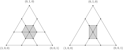
Figure 1: The Wasserstein balls of radius $\frac{1}{6}$ centered in the uniform distribution $(\frac{1}{3},\frac{1}{3},\frac{1}{3})$ associated to the discrete metric (left) and the $L_{1}$-metric (right) for $n=3$.

We now present the optimal value function and the solution function for the model in (2.1). These two functions are piecewise algebraic. The five pieces are shown in Figure 2. On four of them, the solution function is algebraic of degree two. The formula involves a square root in the data distribution. On the fifth piece, the solution function is constant and the optimal value function is linear.

Theorem 1.

For the discrete metric and for the $L_{1}$-metric on the state space $[3]=\{1,2,3\}$, the Wasserstein distance from a data distribution $\mu\in\Delta_{2}$ to the Hardy-Weinberg curve $\mathcal{M}$ equals

$$W_{d}(\mu,\mathcal{M})\,=\,\begin{cases}|2\sqrt{\mu_{1}}-2\mu_{1}-\mu_{2}|&\text{if }\quad\mu_{1}-\mu_{3}\geq 0\text{ and }\mu_{1}\geq\frac{1}{4},\\ |2\sqrt{\mu_{3}}-2\mu_{3}-\mu_{2}|&\text{if }\quad\mu_{1}-\mu_{3}\leq 0\text{ and }\mu_{3}\geq\frac{1}{4},\\ \mu_{2}-\frac{1}{2}&\text{if }\quad\mu_{1}\leq\frac{1}{4}\text{ and }\mu_{3}\leq\frac{1}{4}.\end{cases}$$

The solution function $\,\Delta_{2}\rightarrow\mathcal{M},\,\mu\mapsto\nu^{*}(\mu)\,$ is given (with the same case distinction) by

$$\nu^{*}(\mu)\,=\,\begin{cases}(\mu_{1},2\sqrt{\mu_{1}}-2\mu_{1},1+\mu_{1}-2\sqrt{\mu_{1}}),\\ (1+\mu_{3}-2\sqrt{\mu_{3}},2\sqrt{\mu_{3}}-2\mu_{3},\mu_{3}),\\ (\frac{1}{4},\frac{1}{2},\frac{1}{4}).\end{cases}$$

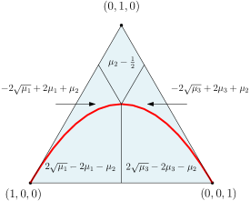
Figure 2: The Hardy-Weinberg curve $\mathcal{M}$ is shown in red. The optimal value function for the Wasserstein distance to this curve is piecewise algebraic with five regions.

Theorem 1 involves a distinction into three cases. Each of the first two cases gives two algebraic pieces of the optimal value function. We point out three interesting features. First, there is a full-dimensional region in $\Delta_{2}$, namely the top parallelogram in Figure 2, all of whose points $\mu$ share the same optimal solution $\nu^{*}(\mu)=(\frac{1}{4},\frac{1}{2},\frac{1}{4})$ in $\mathcal{M}$. Second, all points $\mu$ on the vertical line segment $\{\mu:\mu_{1}=\mu_{3},\mu_{2}<1/2\}$ have two distinct optimal solutions, namely the intersection points of the curve $\mathcal{M}$ with a horizontal line. The identification of such walls of indecision is important for finding accurate numerical solutions. Third, the optimal value and solution functions agree for the two metrics in Figure 1. However, one can perturb the discrete metric to observe a difference. This is illustrated in Figure 3. The point $\mu=(\frac{1}{2},0,\frac{1}{2})$ has two closest points in the $L_{1}$-metric but four closest points in the Wasserstein distance induced by $d=(d_{12},d_{13},d_{23})=(1,1-\epsilon,1)$ for some $\epsilon>0$.

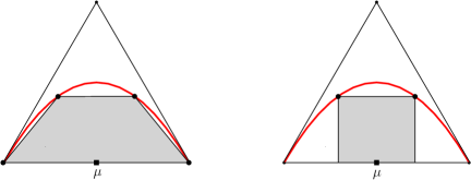
Figure 3: The Wasserstein balls around a data point touch the curve in either four or two points. The metrics on $[3]$ are $d=(1,1-\epsilon,1)$ and $d=(1,2,1)$ respectively.

Next, we increase the dimension by one. Consider the tetrahedron $\Delta_{3}$ whose points are joint probability distributions of two binary random variables $(n=4,k=2)$. The $2$-bit independence model $\mathcal{M}\subset\Delta_{3}$ consists of all nonnegative $2\times 2$ matrices of rank one whose entries sum to one:

$$\qquad\begin{pmatrix}\nu_{1}&\nu_{2}\\ \nu_{3}&\nu_{4}\end{pmatrix}\,=\,\begin{pmatrix}pq&p(1-q)\\ (1{-}p)q&(1{-}p)(1{-}q)\end{pmatrix}\!,\qquad\,(p,q)\in[0,1]^{2}.$$ (2.2)

Thus, $\mathcal{M}$ is the surface in the tetrahedron $\Delta_{3}$ defined by the equation $\nu_{1}\nu_{4}=\nu_{2}\nu_{3}$. We fix the $L_{0}$-metric $d$ on the set of binary pairs $[2]\times[2]$. Under our identification (lexicographic order) of this state space with $[4]=\{1,2,3,4\}$, the resulting metric on $\Delta_{3}$ is given by the $4\times 4$ matrix

$$d\,\,=\,\,\small\begin{pmatrix}\,0&1&1&2\\ \,1&0&2&1\\ \,1&2&0&1\\ \,2&1&1&0\\ \end{pmatrix}.$$ (2.3)

We now present the optimal value function and solution function for this independence model.

Theorem 2.

For the $L_{0}$-metric on the state space $[2]\times[2]$, the Wasserstein distance from a data distribution $\mu\in\Delta_{3}$ to the $2$-bit independence surface $\mathcal{M}$ is given by

$$W_{d}(\mu,\mathcal{M})\,\,=\,\,\begin{cases}2\sqrt{\mu_{1}}(1-\sqrt{\mu_{1}})-\mu_{2}-\mu_{3}&\text{if }\mu_{1}\geq\mu_{4}\,,\,\,\sqrt{\mu_{1}}\geq\mu_{1}+\mu_{2}\,,\,\,\sqrt{\mu_{1}}\geq\mu_{1}+\mu_{3},\vskip 3.0pt plus 1.0pt minus 1.0pt\\ 2\sqrt{\mu_{2}}(1-\sqrt{\mu_{2}})-\mu_{1}-\mu_{4}&\text{if }\mu_{2}\geq\mu_{3}\,,\,\,\sqrt{\mu_{2}}\geq\mu_{1}+\mu_{2}\,,\,\,\sqrt{\mu_{2}}\geq\mu_{2}+\mu_{4},\vskip 3.0pt plus 1.0pt minus 1.0pt\\ 2\sqrt{\mu_{3}}(1-\sqrt{\mu_{3}})-\mu_{1}-\mu_{4}&\text{if }\mu_{3}\geq\mu_{2}\,,\,\,\sqrt{\mu_{3}}\geq\mu_{1}+\mu_{3}\,,\,\,\sqrt{\mu_{3}}\geq\mu_{3}+\mu_{4},\vskip 3.0pt plus 1.0pt minus 1.0pt\\ 2\sqrt{\mu_{4}}(1-\sqrt{\mu_{4}})-\mu_{2}-\mu_{3}&\text{if }\mu_{4}\geq\mu_{1}\,,\,\,\sqrt{\mu_{4}}\geq\mu_{2}+\mu_{4}\,,\,\,\sqrt{\mu_{4}}\geq\mu_{3}+\mu_{4},\vskip 3.0pt plus 1.0pt minus 1.0pt\\ |\mu_{1}\mu_{4}-\mu_{2}\mu_{3}|/(\mu_{1}+\mu_{2})&\text{if }\mu_{1}\geq\mu_{4},\,\mu_{2}\geq\mu_{3},\,\mu_{1}{+}\mu_{2}\geq\sqrt{\mu_{1}},\,\mu_{1}{+}\mu_{2}\geq\sqrt{\mu_{2}},\vskip 3.0pt plus 1.0pt minus 1.0pt\\ |\mu_{1}\mu_{4}-\mu_{2}\mu_{3}|/(\mu_{1}+\mu_{3})&\text{if }\mu_{1}\geq\mu_{4},\,\mu_{3}\geq\mu_{2},\,\mu_{1}{+}\mu_{3}\geq\sqrt{\mu_{1}},\,\mu_{1}{+}\mu_{3}\geq\sqrt{\mu_{3}},\vskip 3.0pt plus 1.0pt minus 1.0pt\\ |\mu_{1}\mu_{4}-\mu_{2}\mu_{3}|/(\mu_{2}+\mu_{4})&\text{if }\mu_{4}\geq\mu_{1},\,\mu_{2}\geq\mu_{3},\,\mu_{2}{+}\mu_{4}\geq\sqrt{\mu_{4}},\,\mu_{2}{+}\mu_{4}\geq\sqrt{\mu_{2}},\vskip 3.0pt plus 1.0pt minus 1.0pt\\ |\mu_{1}\mu_{4}-\mu_{2}\mu_{3}|/(\mu_{3}+\mu_{4})&\text{if }\mu_{4}\geq\mu_{1},\,\mu_{3}\geq\mu_{2},\,\mu_{3}{+}\mu_{4}\geq\sqrt{\mu_{4}},\,\mu_{3}{+}\mu_{4}\geq\sqrt{\mu_{3}}.\end{cases}$$

The solution function $\,\Delta_{3}\rightarrow\mathcal{M},\,\mu\mapsto\nu^{*}(\mu)\,$ is given (with the same case distinction) by

$$\nu^{*}(\mu)\,\,=\,\,\begin{cases}\bigl{(}\,\mu_{1}\,,\,\,\sqrt{\mu_{1}}-\mu_{1}\,,\,\,\sqrt{\mu_{1}}-\mu_{1}\,,\,\,-2\sqrt{\mu_{1}}+\mu_{1}+1\,\bigr{)},\\ \bigl{(}\,\sqrt{\mu_{2}}-\mu_{2}\,,\,\,\mu_{2}\,,\,\,-2\sqrt{\mu_{2}}+\mu_{2}+1\,,\,\,\sqrt{\mu_{2}}-\mu_{2}\,\bigr{)},\\ \bigl{(}\,\sqrt{\mu_{3}}-\mu_{3}\,,\,\,-2\sqrt{\mu_{3}}+\mu_{3}+1\,,\,\,\mu_{3}\,,\,\,\sqrt{\mu_{3}}-\mu_{3}\,\bigr{)},\\ \bigl{(}\,-2\sqrt{\mu_{4}}+\mu_{4}+1\,,\,\,\sqrt{\mu_{4}}-\mu_{4}\,,\,\,\sqrt{\mu_{4}}-\mu_{4}\,,\,\,\mu_{4}\,\bigr{)},\\ \bigl{(}\,\mu_{1}\,,\,\,\mu_{2}\,,\,\,\mu_{1}(\mu_{3}{+}\mu_{4})/(\mu_{1}{+}\mu_{2})\,,\,\,\mu_{2}(\mu_{3}{+}\mu_{4})/(\mu_{1}{+}\mu_{2})\,\bigr{)},\\ \bigl{(}\,\mu_{1}\,,\,\,\mu_{1}(\mu_{2}{+}\mu_{4})/(\mu_{1}{+}\mu_{3})\,,\,\,\mu_{3}\,,\,\,\mu_{3}(\mu_{2}{+}\mu_{4})/(\mu_{1}{+}\mu_{3})\,\bigr{)},\\ \bigl{(}\,\mu_{2}(\mu_{1}{+}\mu_{3})/(\mu_{2}{+}\mu_{4})\,,\,\,\mu_{2}\,,\,\,\mu_{4}(\mu_{1}{+}\mu_{3})/(\mu_{2}{+}\mu_{4})\,,\,\,\mu_{4}\,\bigr{)},\\ \bigl{(}\,\mu_{3}(\mu_{1}{+}\mu_{2})/(\mu_{3}{+}\mu_{4})\,,\,\,\mu_{4}(\mu_{1}{+}\mu_{2})/(\mu_{3}{+}\mu_{4})\,,\,\,\mu_{3}\,,\,\,\mu_{4}\,\bigr{)}.\end{cases}$$

The walls of indecision are the surfaces $\{\mu\in\Delta_{3}:\mu_{1}-\mu_{4}=0,\mu_{1}+\mu_{2}\geq\sqrt{\mu_{1}},\mu_{1}+\mu_{3}\geq\sqrt{\mu_{1}}\}$ and $\{\mu\in\Delta_{3}:\mu_{2}-\mu_{3}=0,\mu_{1}+\mu_{2}\geq\sqrt{\mu_{2}},\mu_{2}+\mu_{4}\geq\sqrt{\mu_{2}}\}$.

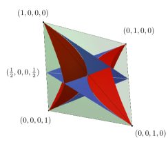
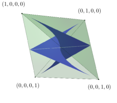
Figure 4: The optimal value function of Theorem 2 subdivides the tetrahedron of probability distributions $\mu$ (left). The walls of indecision are shown in blue (right).

Theorem 2 distinguishes eight cases. This division of $\Delta_{3}$ is shown in Figure 4. Each of the last four cases breaks into two subcases, since the numerator in the formulas is the absolute value of $\mu_{1}\mu_{4}-\mu_{2}\mu_{3}$. The sign of this $2\times 2$ determinant matters for the pieces of our piecewise algebraic function. The tetrahedron $\Delta_{3}$ is divided into $12$ regions on which $\mu\mapsto W_{d}(\mu,\mathcal{M})$ is algebraic.

We now explain Figure 4. The red surface consists of eight pieces. Together with the blue surface, these separate the eight cases (this surface is not the model). Four convex regions are enclosed between the red surfaces and the sides they meet. These regions represent the first four cases in Theorem 2. For instance, the region containing the points $(1,0,0,0),(1/2,0,0,1/2)$ corresponds to the first case. The remaining four regions are each bounded by two red and two blue pieces, and correspond to the last four cases. Each of these four regions is further split in two by the model which we do not depict for the sake of visualization. The two sides are determined by the sign of the determinant $\mu_{1}\mu_{4}-\mu_{2}\mu_{3}$. The two blue shapes in the right figure form the walls of indecision. These specify the points $\mu\in\Delta_{3}$ with more than one optimal solution.

The same 2-bit model was studied in our conference paper [2]. Theorem 2 is a much improved representation of the results in [2, Table 2]. Our formulas can easily be translated into a description in terms of the parameters $(p,q)$ from (2.2). The linear program we used in (1.1) to define the Wasserstein distance is dual to the one via optimal transport in [2, eqn (2)]. The latter primal formulation underlies the analysis in [2, §5]. In Section 3, we will present a self-contained proof of Theorem 2 after a general discussion of distance minimization for polyhedral norms.

3 Polyhedral Norm Distance to a Variety

The Wasserstein metric on the simplex of probability distributions with $n$ states defines a polyhedral norm on $\mathbb{R}^{m}$ with $m=n-1$ as follows. We translate the simplex $\Delta_{m}$ such that its barycenter is the origin. Next we consider a Wasserstein unit ball around the origin, denoted by $B$. This unit ball is a centrally symmetric $m$-dimensional polytope $B$. It induces a norm on $\mathbb{R}^{m}$ by

$$\|y\|_{B}\,\,\,:=\,\,\,{\rm min}\,\{\,\lambda\in\mathbb{R}_{\geq 0}\,:\,y\in\lambda B\,\}.$$

In terms of the dual polytope

$$B^{*}\,\,=\,\,\{\,x\in\mathbb{R}^{m}\,:\,\sup_{z\in B}\langle x,z\rangle\leq 1\,\},$$

the polyhedral norm can be rewritten as

$$\|y\|_{B}\,\,\,=\,\,\,{\rm min}\,\{\,\lambda\in\mathbb{R}_{\geq 0}\,:\,\sup_{x\in B^{*}}\langle x,y\rangle\leq\lambda\,\}\,\,\,=\,\,\,\max_{x\in B^{*}}\,\langle x,y\rangle.$$

Note that $(B^{*})^{*}=B$. The dual of the unit ball equals

$$B^{*}\,\,=\,\,P_{d}\,\,=\,\,\bigl{\{}\,x\in\mathbb{R}^{n}/\mathbb{R}{\bf 1}\,\,:\,\,\,|x_{i}-x_{j}|\,\leq\,d_{ij}\,\,\,\,\text{for all}\,\,\,1\leq i<j\leq n\,\bigr{\}}.$$

This is the Lipschitz polytope in (1.2), and the unit ball $B=P_{d}^{*}$ is its dual. This means that the Wasserstein unit ball $B$ is the convex hull of $n(n-1)$ vectors that lie on a hyperplane in $\mathbb{R}^{n}$:

$$B\,\,=\,\,P_{d}^{*}\,\,=\,\,\,{\rm conv}\,\biggl{\{}\,\frac{1}{d_{ij}}(e_{i}-e_{j})\,\,:\,\,\,\,1\leq i<j\leq n\,\biggr{\}}.$$

In the case $m=n-1=2$, two Wasserstein balls for different metrics $d$ were shown in Figure 1.

Example 3.

Fix $m=n-1=3$ and let $d$ be the $2$-bit Hamming metric in (2.3). We work in the linear space $L$ that is defined by $x_{1}+x_{2}+x_{3}+x_{4}=0$. The Lipschitz polytope is the octahedron

$$P_{d} =B^{*}=\,\,\bigl{\{}\,(x_{1},x_{2},x_{3},x_{4})\in L\,:\,|x_{1}-x_{2}|\leq 1,\,|x_{1}-x_{3}|\leq 1,\,|x_{2}-x_{4}|\leq 1,\,|x_{3}-x_{4}|\leq 1\,\bigr{\}}$$

$$={\rm conv}\bigl{\{}(1,0,0,-1),(1,0,0,-1),(\tfrac{1}{2},-\tfrac{1}{2},-\tfrac{1}{2},\tfrac{1}{2}),(-\tfrac{1}{2},\tfrac{1}{2},\tfrac{1}{2},-\tfrac{1}{2}),(0,1,-1,0),(0,-1,1,0)\bigr{\}}.$$

The Wasserstein unit ball is the cube

$$\begin{matrix}B\,=\,P_{d}^{*}&\!\!=\!&\bigl{\{}\,(y_{1},y_{2},y_{3},y_{4})\in L\,:\,|y_{1}-y_{4}|\leq 1,\,|y_{2}-y_{3}|\leq 1,\,|y_{2}+y_{3}|\leq 1\bigr{\}}\\ &\!\!=\!&{\rm conv}\bigl{\{}(1,-1,0,0),(1,0,-1,0),(0,1,0,-1),(0,0,1,-1)\\ &&(-1,1,0,0),(-1,0,1,0),(0,-1,0,1),(0,0,-1,1)\bigr{\}}.\end{matrix}$$

Returning to the general case, suppose that $\mathcal{M}$ is a smooth compact algebraic variety in $\mathbb{R}^{m}$. For any point $u\in\mathbb{R}^{m}$, we are interested in its distance to the variety under our polyhedral norm:

$$D_{B}(u,\mathcal{M})\,\,\,:=\,\,\,{\rm min}\bigl{\{}\,\|u-v\|_{B}\,:\,v\in\mathcal{M}\,\bigr{\}}\,\,\,=\,\,\,{\rm min}\bigl{\{}\,\lambda\in\mathbb{R}_{\geq 0}\,:\,(u+\lambda B)\,\cap\,\mathcal{M}\,\not=\,\emptyset\,\bigr{\}}.$$

We will now embark on understanding the geometry of this optimization problem.

Proposition 4.

If the model $\mathcal{M}$ and the point $u$ are in general position relative to the unit ball $B$ then there is a unique optimal point $v\in\mathcal{M}$ for which $D_{B}(u,\mathcal{M})=\|u-v\|_{B}=\lambda$ holds. The point $\frac{1}{\lambda}(v-u)$ is in the relative interior of a unique face $F$ of the polytope $B$; we say that $v$ has type $F$.

The general position hypothesis is understood as follows. The rotation group and the translation group act on $\mathbb{R}^{m}$. These two algebraic groups have Zariski dense subsets such that the hypothesis holds after applying group elements from those two subsets to $\mathcal{M}$ and $u$ respectively.

Proof.

We have $\lambda=D_{B}(u,\mathcal{M})$, so $\frac{1}{\lambda}(v-u)$ lies in the boundary of the unit ball $B$. The polytope $B$ is the disjoint union of the relative interior of its faces. Hence there exists a unique face $F$ that has $\frac{1}{\lambda}(v-u)$ in its relative interior. Let $L_{F}$ be the linear subspace of $\mathbb{R}^{m}$ that consists of linear combinations of vectors in $F$. By hypothesis, the resulting affine subspace $u+L_{F}$ intersects the variety $\mathcal{M}$ transversally, and $v$ is a general smooth point in that intersection. Moreover, $v$ is a minimum of the restriction to the variety $(u+L_{F})\cap\mathcal{M}$ of a linear function on $u+L_{F}$. Our hypothesis ensures that the linear function is generic relative to the variety, which in turn is smooth and compact. The number of critical points is finite. This guarantees that the linear function attains its minimum at a unique point in the variety, namely at $v$. ∎

Our geometric discussion becomes very concrete in the Wasserstein case. The data point is $u=\mu$ and the optimal point is $v=\nu^{*}$. The type of $v$ is a face $F$ of the unit ball $B=P_{d}^{*}$. Fix the face $F$. This allows for the following algebraic characterization of optimality. Let $\mathcal{F}$ be the set of all index pairs $(i,j)$ such that the point $\frac{1}{d_{ij}}(e_{i}-e_{j})$ is a vertex and it lies in $F$. Let $\ell_{F}$ be any linear functional on $\mathbb{R}^{m}$ that attains its maximum over $B$ at $F$. We work in the linear space

$$L_{F}\,\,\,=\,\,\,\left\{\,\sum_{(i,j)\in\mathcal{F}}\!\!\lambda_{ij}(e_{i}-e_{j})\,\,:\,\,\lambda_{ij}\in\mathbb{R}\,\right\}.$$ (3.1)

The point $\nu^{*}$ on $\mathcal{M}$ that is closest to $\mu$ is the solution of the following optimization problem:

Minimize $$\,\ell_{F}=\ell_{F}(\nu)\, \,\nu\in(\mu+L_{F})\cap\mathcal{M}$$ subject to . (3.2)

This is a polynomial optimization problem in the linear subspace $L_{F}$ of $\mathbb{R}^{m}$. With the notation in (3.1), the decision variables are $\lambda_{ij}$ for $(i,j)\in\mathcal{F}$. The algebraic complexity of this problem will be studied in Section 5. In Section 4, we focus on the combinatorial complexity. The unit ball $B$ has very many faces, and our desire is to control that combinatorial explosion. For the remainder of this section, we return to the three-dimensional case seen in Section 2, and we present a proof of Theorem 2 that uses the set-up above. Theorem 1 is analogous and its proof will be omitted.

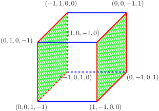
Figure 5: Subdivision of the faces of the Wasserstein ball as in the proof of Theorem 2.

Proof of Theorem 2.

The Wasserstein unit ball is the cube $B$ in Example 3. We must solve (3.2) for every face $F$ of $B$. There are various symmetries we can employ to simplify the proof. First, since $B$ is centrally symmetric, we study only one among a face $F$ and its negative $-F$. Since $L_{F}=L_{-F}$, minima in (3.2) for $F$ turn into maxima for $-F$, and vice versa. Second, consider the dihedral group $D_{4}$ of order $8$ that is generated by the involutions $(14)$ and $(12)(34)$ in the symmetric group on $\{1,2,3,4\}$. This acts on the tetrahedron $\Delta_{3}$, on the cube $B$, and on the model $\mathcal{M}$, by permuting coordinates in $\mathbb{R}^{4}$. The action respects scalar products: $\langle c,x\rangle=\langle g\cdot c,g\cdot x\rangle$ for every $g\in D_{4}$. Therefore, $g\cdot F$ is a face of $B$ for every face $F$ and every $g\in D_{4}$, and the problem (3.2) is symmetric under $D_{4}$. The solution function satisfies $\,\nu^{*}(g\cdot\mu)=g\cdot\nu^{*}(\mu)\,$ for all $g\in D_{4}$.

For each vertex, edge or $2$-face, one per symmetry class, we introduce Lagrange multipliers to compute the critical points of (3.2). In each case, there are at most two critical points, since the polar degrees are $\delta=(2,2,2)$; see $k=2$ in Table 2. We now undertake a case-by-case analysis:

• $\dim(F)=2$: The green facets in Figure 5 give two orbits. For the first facet, Lagrange multipliers reveal a critical point $\nu^{*}=(1/4,1/4,1/4,1/4)$. However, the associated constrained Hessian is indefinite, and hence $\nu^{*}$ is not a local minimum. The second facet has no critical points in $\Delta_{3}$. Hence there is never any optimal solution whose type is a facet.

• $\dim(F)=1$: We have two orbits of edges, marked in red (bounding the green facets) and blue in Figure 5. Representatives are $E_{1}=\operatorname{conv}\{(-1,1,0,0),(-1,0,1,0)\}$ and $E_{2}=\operatorname{conv}\{(1,-1,0,0),(0,0,1,-1)\}$. For the first, we have $L_{E_{1}}=\{x_{4}=0,x_{1}+x_{2}+x_{3}=0\}$ and $\ell_{E_{1}}=-x_{1}+x_{4}$. The associated Lagrangian system has two solutions one of which is contained in $\Delta_{3}$, namely $\nu^{*}=(-2\sqrt{\mu_{4}}+\mu_{4}+1,\sqrt{\mu_{4}}-\mu_{4},\sqrt{\mu_{4}}-\mu_{4},\mu_{4})$. The constrained Hessian reveals that $\nu^{*}$ is a local minimum. It remains to determine the constraints of the region on which $\nu^{*}$ lies in the interior of $E_{1}$. They can be obtained from the inequalities defining the $2$-dimensional cone

  $$C_{E_{1}}\,\,:=\,\,\{\,\lambda_{12}(e_{2}-e_{1})+\lambda_{13}(e_{3}-e_{1})\,\,:\,\,\lambda_{12},\lambda_{13}\in\mathbb{R}_{\geq 0}\,\}.$$

  Then $\nu^{*}\in\mu+C_{E_{1}}$ if and only if $\nu^{*}_{2}-\mu_{2}\geq 0$ and $\nu^{*}_{3}-\mu_{3}\geq 0$, that is $\sqrt{\mu_{4}}-\mu_{4}-\mu_{2}\geq 0$ and $\sqrt{\mu_{4}}-\mu_{4}-\mu_{3}\geq 0$. As $\ell_{E_{1}}=-x_{1}+x_{4}$, the corresponding optimal Wasserstein distance is

  $$\quad W(\mu,\nu^{*})\,\,\,=\,\,\,\ell_{E_{1}}(\nu^{*}-\mu)\,\,\,=\,\,\,2\sqrt{\mu_{4}}+\mu_{1}-\mu_{4}-1\,\,=\,\,2\sqrt{\mu_{4}}(1-\sqrt{\mu_{4}})-\mu_{2}-\mu_{3}.$$

  The optimization problem associated to $E_{2}$ does not have critical points.

• $\dim(F)=0$: The eight vertices of $B$ form one orbit. We consider $v=(1,-1,0,0)$, with associated zero-dimensional variety $(\mu+L_{v})\cap\mathcal{M}$. This consists of a unique point $\nu^{*}=(\frac{\mu_{3}(\mu_{1}+\mu_{2})}{\mu_{3}+\mu_{4}},\frac{\mu_{4}(\mu_{1}+\mu_{2})}{\mu_{3}+\mu_{4}},\mu_{3},\mu_{4})$. Depending on $\mu$, this point can lie either on the ray through $\mu+v$, denoted $\mu+C_{v}$, or on the ray through $\mu-v$. We have $\nu^{*}\in(\mu+C_{v})\cap\mathcal{M}$ if and only if $\nu^{*}_{1}-\mu_{1}\geq 0$, that is $\frac{\mu_{2}\mu_{3}-\mu_{1}\mu_{4}}{\mu_{3}+\mu_{4}}\geq 0$. In this case we choose $\ell_{v}=-x_{2}-x_{3}$, and we obtain

  $$W(\mu,\nu^{*})\,\,\,=\,\,\,\ell_{v}(\nu^{*}-\mu)\,\,\,=\,\,\,-\frac{\mu_{4}(\mu_{1}+\mu_{2})}{\mu_{3}+\mu_{4}}-\mu_{3}+\mu_{2}+\mu_{3}\,\,\,=\,\,\,\frac{\mu_{2}\mu_{3}-\mu_{1}\mu_{4}}{\mu_{3}+\mu_{4}}.$$

We act with the dihedral group $D_{4}$ on the two local minima we found. This yields the eight expressions for $\nu^{*}$ shown in Theorem 2. It remains to decide which point $\nu^{*}$ is the global minimum. This is done by pairwise comparison of the eight expressions for the Wasserstein distance $W_{d}(\mu,\nu^{*})$. We omit this last step, since it consists of elementary algebraic manipulation. ∎

4 Lipschitz polytopes

The combinatorial complexity of our problem is governed by the facial structure of the Wasserstein ball given by a finite metric space $([n],d)$. We now focus on the polar dual of that ball, which is the Lipschitz polytope $\,P_{d}$. This lives in $\,\mathbb{R}^{n}/\mathbb{R}{\bf 1}\simeq\mathbb{R}^{n-1}$, and is defined in (1.2).

This object appears in the literature in several guises. See e.g. [9] for a study that emphasizes generic distances $d_{ij}$. We consider specific metrics that are relevant for the independence model:

• The discrete metric on any finite set $[n]$ where $\,d_{ij}=1$ for distinct $i,j$.

• The $L_{0}$-metric on $[m_{1}]\times\dots\times[m_{k}]$ where $\,d_{ij}=\#\{l:i_{l}\neq j_{l}\}$.

• The $L_{1}$-metric on $[m_{1}]\times\dots\times[m_{k}]$ where $\,d_{ij}=\sum_{l=1}^{k}|i_{l}-j_{l}|$.

For the last two metrics we have $n=m_{1}\cdots m_{k}$. To compute the Wasserstein distance in each case, we need to describe the Lipschitz polytope $P_{d}$ as explicitly as possible. All three metrics above can be interpreted as graph metrics. This means that there exists an undirected simple graph $G$ with vertex set $[n]$ such that $d_{ij}$ is the length of the shortest path from $i$ to $j$ in $G$. Wasserstein balls associated to graphs in this way are studied in [4] under the name symmetric edge polytopes.

For the discrete metric on $[n]$, the graph is the complete graph $K_{n}$. In the case of the $L_{0}$-metric on $[m_{1}]\times\dots\times[m_{k}]$, we have the Cartesian product of complete graphs $K_{m_{1}}\times\dots\times K_{m_{k}}$. In the last case, the corresponding graph is the Cartesian product of paths of length $m_{1},\dots,m_{k}$. The facets of the Lipschitz polytope $P_{d}$ arising from a graph $G$ correspond to the edges of $G$. We have

$$P_{d}\,\,=\,\,\{\,x\in\mathbb{R}^{n}/\mathbb{R}{\bf 1}\,:\,|x_{i}-x_{j}|\leq 1\,\text{ for every edge }(i,j)\,\,{\rm of}\,\,G\,\}.$$ (4.1)

This representation of $P_{d}$ is a consequence of the triangle inequality. Vertices of $P_{d}$ are precisely those points for which at least $\dim(P_{d})$ inequalities are sharp. More generally, we are interested in higher-dimensional faces of $P_{d}$. The number of $i$-dimensional faces of $P_{d}$ is denoted by $f_{i}=f_{i}(P_{d})$, and we write $f=(f_{0},f_{1},\ldots,f_{n-2})$ for the f-vector. Since $P_{d}$ is $(n-1)$-dimensional, we have $f_{n-1}(P_{d})=1$, and we omit this number. In general, it is difficult to compute the $f$-vector.

If $d$ is the discrete metric on $[n]$, then we have the following description of the faces. The corresponding Lipschitz polytope $P_{d}$ is a zonotope, namely it is the Minkowski sum of $n$ general segments in $(n-1)$-space. For $n=4$ this is the rhombic dodecahedron [11, Figure 4]. Its dual, the Wasserstein ball for the discrete metric on $[n]$, is the root polytope of Lie type A; cf. [11, 16].

Lemma 5.

Let $d$ be the discrete metric on $[n]$. The vertices of $P_{d}$ are the binary vectors $\sum_{i\in I}e_{i}$ where $I$ runs over elements of the power set $\,2^{[n]}\backslash\{\emptyset,[n]\}$. Furthermore, a subset $\,S$ of $2^{[n]}\backslash\{\emptyset,[n]\}$ indexes the vertices of a face of $P_{d}$ if and only if $\,S=\{I:L\subseteq I\subseteq U\}$ for some $L,U\in 2^{[n]}\backslash\{\emptyset,[n]\}$.

Proof.

Clearly, $e_{I}=\sum_{i\in I}e_{i}$ lies in $P_{d}$. We observe that $(e_{I})_{i}-(e_{I})_{j}=1$ if and only if $i\in I$ and $j\notin I$. The corresponding linear forms $x_{i}-x_{j}$ for $i\in I$ and $j\not\in I$ span an $(n-1)$-dimensional space. This means that $e_{I}$ is a vertex of $P_{d}$. Conversely, there are no vertices other than the $e_{I}$ since $v_{i}-v_{j}=1$ implies $v_{i}=1$ and $v_{j}=0$ for $v\in\mathbb{R}^{n}/\mathbb{R}{\bf 1}$. For the second statement, consider any linear functional $\ell$ on $P_{d}$. We have $\ell=\sum_{i=1}^{n}a_{i}x_{i}$ where $\sum_{i=1}^{n}a_{i}=0$. Set $L=\{i:a_{i}>0\}$ and $U=\{i:a_{i}\geq 0\}$. Then $\ell$ is maximized over $P_{d}$ at the convex hull of $\{e_{I}\,:\,L\subseteq I\subseteq U\}$, so this is a face. Every face is the set of maximizers of a linear functional on $P_{d}$. This proves the claim. ∎

From this description of $P_{d}$ we can read off the number of faces in each dimension.

Corollary 6.

[3, Proposition 4.3] Let $d$ be the discrete metric on $[n]$. Then

$$f_{i}(P_{d})\,=\,f_{n-i-2}(P_{d}^{*})\,\,=\,\,\binom{n}{i}(2^{n-i}-2)\qquad\hbox{ for $\,i=0,\dots,n-2$.}$$

Proof.

The face indexed by $(L,U)$ in the proof of Lemma 5 has dimension $|U|-|L|$. Hence $f_{i}$ is the number of chains $\,\emptyset\subsetneq L\subseteq U\subsetneq[n]\,$ with $|U|-|L|=i$. This is the given number. ∎

Example 7 ($n=4$).

We consider the discrete metric on $[4]=\{1,2,3,4\}$. The $3$-dimensional Lipschitz polytope $P_{d}$ is the rhombic dodecahedron with $f$-vector $(14,24,12)$. Its dual $P_{d}^{*}$ is the Wasserstein ball with $f$-vector $(12,24,14)$. The normal fan of $P_{d}$, which is the fan over $P_{d}^{*}$, is a central arrangement of four general planes in a $3$-dimensional space. This has $14$ regions.

Corollary 8.

Up to a factor of 2, the Wasserstein distance between probability distributions on $[n]$ is the restriction of the $L_{1}$-distance on $\mathbb{R}^{n}$. In symbols $W_{d}=\frac{1}{2}\|\mu-\nu\|_{L_{1}}$ for $\mu,\nu\in\Delta_{n-1}$.

Proof.

Up to a factor of $2$, which we ignore, $P_{d}$ is the image of the cube $[-1,1]^{n}$ under the map $\mathbb{R}^{n}\rightarrow\mathbb{R}^{n}/\mathbb{R}\mathbf{1}$. Hence its dual, which is the $L_{1}$-ball or cross polytope, intersects the hyperplane $\mathbf{1}^{\perp}$ in the Wasserstein ball $P_{d}^{*}$. This means that the $L_{1}$-metric agrees with the Wasserstein metric on any translate of $\mathbf{1}^{\perp}$. More explicitly, we compute $W_{d}(\mu,\nu)$ with the formula (1.1). This yields

$$W_{d}(\mu,\nu)\,\,=\,\,\max_{x\in P_{d}}\langle\mu-\nu,x\rangle\,\,=\,\,\langle\mu-\nu,\text{sign}(\mu-\nu)\rangle\,\,=\,\,\sum_{i=1}^{n}|\mu_{i}-\nu_{i}|.$$

Here we identify the linear functionals given by the vertices of $2P_{d}$ with elements in $\{-1,1\}^{n}$. ∎

Example 9.

The $L_{1}$-ball for $n=3$ is an octahedron. The restriction of this octahedron to the triangle $\Delta_{2}$ is the hexagon on the left of Figure 1.

We next examine the Lipschitz polytope $P_{d}$ for metrics associated to graphs $G$ other than $K_{n}$. The inequality representation was given in (4.1). However, describing all faces, or even just the vertex set $V(P_{d})$, is now more difficult than in Lemma 5. The Wasserstein ball $P_{d}^{*}$ is the convex hull of the subset of vertices $e_{i}-e_{j}$ of the root polytope of type A that are indexed by edges of $G$. The following result for bipartite graphs $G$ is due to [4, Lemma 4.5]. A related characterization for weighted graphs was obtained in [12, Theorem 2, §3.1].

Proposition 10.

Let $d$ be a graph metric where $G$ is bipartite. The set of vertices of $P_{d}$ equals

$$V(P_{d})\,\,=\,\,\{\,x\in\mathbb{Z}^{n}/\mathbb{Z}{\bf 1}\,:\,|x_{i}-x_{j}|=1\,\text{ for every edge }(i,j)\,\,{\rm of}\,\,G\,\}.$$ (4.2)

Proposition 10 covers the case of the Lipschitz polytope for the $L_{1}$-norm on a product of finite sets. In particular, we obtain a vertex description for the Lipschitz polytope of the graph of the $k$-cube. This covers the $L_{0}$-metric which is equal to the $L_{1}$-metric on the states of the $k$-bit models. This metric is the Hamming distance on a cube. In Example 3, we described this for the $2$-bit model, for which the Lipschitz polytope is an octahedron, and its dual is a cube.

It is not easy to compute the cardinality of (4.2). In graph theory, this corresponds to counting graph homomorphisms from the $k$-cube to the infinite path with a fixed point. [6] observed that there is a bijection between $V(P_{d})$ and the proper $3$-colorings of $k$-cube with a vertex with fixed color. For $k=2,3,4,5,6$, the corresponding number equals $\,6,\,38,\,990,\,395094,\,33433683534$. This was computed with the graph coloring code in SageMath. We refer to [6] for asymptotics.

It follows from results in [11] that the Wasserstein ball for the discrete metric on $[n]$ has the most vertices for any metric on $[n]$. We next discuss the Wasserstein ball with the fewest vertices.

Example 11.

Let $d$ be the $L_{1}$-metric on $[n]$, i.e. the graph metric of the $n$-path. Then $\,P_{d}\,=\,\{|x_{i}-x_{i+1}|\leq 1\,:\,i=1,2,\ldots,n-1\}\,$ is combinatorially an $(n-1)$-cube, and $P_{d}$ is a cross polytope. This has the minimum number of vertices for any centrally symmetric $(n-1)$-polytope:

$$\qquad f_{i}(P_{d})\,=\,f_{n-i-2}(P_{d}^{*})\,=\,2^{n-i-1}\binom{n-1}{i}\qquad\hbox{for}\,\,\,i=0,1,\dots,n-2.$$

We conclude this section with four independence models that serve as examples for our case studies in the next sections. The tuple $(({m_{1}})_{d_{1}},\dots,({m_{k}})_{d_{k}})$ denotes the independence model with $n=\prod_{i=1}^{k}\binom{m_{i}+d_{i}-1}{d_{i}}$ states where the $i$th entry $(m_{i})_{d_{i}}$ refers to a multinomial distribution with $m_{i}$ possible outcomes and $d_{i}$ trials. This can be interpreted as an unordered set of $d_{i}$ identically distributed random variables on $[m_{i}]=\{1,2,...,m_{i}\}$. The subscript $d_{i}$ is omitted if $d_{i}=1$.

For example, $(2_{2},2)$ denotes the independence model for three binary random variables where the first two are identically distributed. We list the $n=6$ states in the order $00,10,20,01,11,21$. These are the vertices of the associated graph $G$, which is the product of a $3$-chain and a $2$-chain. This model $\mathcal{M}$ is the image of the map from the square $[0,1]^{2}$ into the simplex $\Delta_{5}$ given by

$$(p,q)\,\mapsto\,\bigl{(}\,p^{2}q,\,2p(1-p)q,\,(1-p)^{2}q,\,p^{2}(1-q),\,2p(1-p)(1-q),\,(1-p)^{2}(1-q)\,\bigr{)}.$$ (4.3)

Example 12.

Our four models are: the $3$-bit model $(2,2,2)$ with the $L_{0}$-metric on $[2]^{3}$; the model $(3,3)$ for two ternary variables with the $L_{1}$-metric on $[3]^{2}$; the model $(2_{6})$ for six identically distributed binary variables with the discrete metric on $[7]$; the model $(2_{2},2)$ in (4.3) with the $L_{1}$-metric on $[3]\times[2]$. In Table 1, we report the $f$-vectors of the corresponding Wasserstein balls.

$\mathcal{M}$	$n$	$\dim(\mathcal{M})$	Metric $d$	$f$-vector of the $(n{-}1)$-polytope $P_{d}^{*}$
$(2,2,2)$	8	3	$L_{0}=L_{1}$	$(24,192,652,1062,848,306,38)$
$(3,3)$	9	4	$L_{1}$	$(24,216,960,2298,3048,2172,736,82)$
$(2_{6})$	7	1	discrete	$(42,210,490,630,434,126)$
$(2_{2},2)$	6	2	$L_{1}$	$(14,60,102,72,18)$

Table 1: $f$-vectors of the Wasserstein balls for the four models in Example 12.

5 Polar Degrees of Independence Models

In this section, we examine the problem (3.2) for fixed type $F$ from the perspective of algebraic geometry. Given a compact smooth algebraic variety $\mathcal{M}$ in $\mathbb{R}^{m}$, we consider a linear functional $\ell$ and an affine-linear space $L$ of dimension $r$ in $\mathbb{R}^{m}$. It is assumed that the pair $(\ell,L)$ is in general position relative to $\mathcal{M}$. Our aim is to study the following optimization problem:

$$\hbox{Minimize the linear functional}\,\,\,\ell\,\,\,\hbox{over the intersection}\,\,L\,\cap\,\mathcal{M}\,\,{\rm in}\,\,\mathbb{R}^{m}.$$ (5.1)

This is a constrained optimization problem. We write the critical equations as a system of polynomial equations. Its unknowns are the $m$ coordinates of $\mathbb{R}^{m}$ plus various Lagrange multipliers. The genericity assumption allows us to attach an algebraic degree to this optimization problem. That degree is the number of complex solutions to the critical equations. Assuming $(\ell,L)$ to be generic, this number does not depend on the choice of $(\ell,L)$ but just on the dimension $r$ of $L$. The following result furnishes a recipe for assessing the algebraic complexity of our problem.

Theorem 13.

The algebraic degree of the problem (5.1) is the polar degree $\delta_{r}$ of $\mathcal{M}$.

We begin by explaining this statement. First of all, we already tacitly replaced $\mathcal{M}$ by its closure in complex projective space $\mathbb{P}^{m}$, and we are assuming that this projective variety is smooth. Let $(\mathbb{P}^{m})^{\vee}$ denote the dual projective space whose points are the hyperplanes $h$ in $\mathbb{P}^{m}$. The conormal variety of the model $\mathcal{M}$ is the following subvariety in the product of two projective spaces:

$$CV(\mathcal{M})\quad=\quad\bigl{\{}\,(x,h)\in\mathbb{P}^{m}\times(\mathbb{P}^{m})^{\vee}\,\,:\,\,\hbox{the point $x$ lies in $\mathcal{M}$ and $h$ is tangent to $\mathcal{M}$ at $x$}\,\bigr{\}}.$$

The importance of the conormal variety for optimization has been explained in several sources, including [5, 13, 14]. The projection of $CV(\mathcal{M})$ onto the second factor $(\mathbb{P}^{m})^{\vee}$ is the dual variety $\mathcal{M}^{*}$, which parametrizes hyperplanes that are tangent to $\mathcal{M}$. It is known that $CV(\mathcal{M}^{*})=CV(\mathcal{M})$ and that this conormal variety always has dimension $m-1$; see [14, Proposition 2.4 and Theorem 2.6]. The dual variety already appeared in [2, §4], but here we need a more general approach.

Let $[CV(\mathcal{M})]$ denote the class of the conormal variety in the cohomology of $\mathbb{P}^{m}\times(\mathbb{P}^{m})^{\vee}$. This cohomology ring is $\mathbb{Z}[s,t]/\langle s^{m+1},t^{m+1}\rangle$, and hence the class $[CV(\mathcal{M})]$ is a homogeneous polynomial of degree $m+1$ in two unknowns $s$ and $t$. We can write this binary form as follows:

$$[CV(\mathcal{M})]\quad=\quad\sum_{r=1}^{m}\,\delta_{r-1}\cdot s^{r}t^{m+1-r}.$$ (5.2)

The coefficients $\delta_{0},\delta_{1},\delta_{2},\ldots$ are the polar degrees of the model $\mathcal{M}$. Some of these are zero. Namely, the sum in (5.2) ranges from $r_{1}$ to $r_{2}$, where ${\rm dim}(\mathcal{M})=m-r_{1}$ and ${\rm dim}(\mathcal{M}^{*})=r_{2}$. The first and last non-zero coefficients are $\delta_{r_{1}-1}={\rm degree}(\mathcal{M})$ and $\delta_{r_{2}-1}={\rm degree}(\mathcal{M}^{*})$ respectively.

Proof of Theorem 13.

It is known that $\delta_{r-1}$ equals the number of points in $(L_{r}\times L^{\prime}_{m+1-r})\cap CV(\mathcal{M})$ where $L_{r}\subset\mathbb{P}^{m}$ is a general linear space of dimension $r$ and $L^{\prime}_{m+1-r}\subset(\mathbb{P}^{m})^{\vee}$ is a general linear space of dimension $m{+}1{-}r$; see e.g. [5, §5]. We now identify $L_{r}$ with the linear space $L$ in (5.1). The intersection $(L_{r}\times(\mathbb{P}^{m})^{\vee})\,\cap\,CV(\mathcal{M})$ is a smooth variety of dimension $r-1$ by Bertini’s Theorem. In (5.1), we optimize a general linear functional over its projection into the first factor $\mathbb{P}^{m}$. The dual variety to that projection lives in $(\mathbb{P}^{m})^{\vee}$, and the desired algebraic degree is the degree of the dual variety. This is obtained geometrically by intersecting with $L^{\prime}_{m+1-r}$. ∎

The independence models treated in this article are known in algebraic geometry as Segre-Veronese varieties. The study of characteristic classes for these families is a classical subject in algebraic geometry. The explicit computation of these polar degrees was carried out only recently, in the doctoral dissertation [15]. The result is described in Theorem 14 below.

Let $\mathcal{M}$ be the model denoted $(({m_{1}})_{d_{1}},\dots,({m_{k}})_{d_{k}})$ in Section 4. The corresponding Segre-Veronese variety is the embedding of $\mathbb{P}^{m_{1}-1}\times\dots\times\mathbb{P}^{m_{k}-1}$ in the space of partially symmetric tensors, $\,\mathbb{P}({\rm Sym}_{d_{1}}\mathbb{R}^{m_{1}}\otimes\dots\otimes{\rm Sym}_{d_{k}}\mathbb{R}^{m_{k}})$. That projective space equals $\mathbb{P}^{n-1}$ where $n=\prod_{i=1}^{k}\binom{m_{i}+d_{i}-1}{d_{i}}$. We identify its real nonnegative points with the simplex $\Delta_{n-1}$. The independence model $\mathcal{M}$ consists of the rank one tensors. Its dimension is denoted $\,{\bf m}:=(m_{1}-1)+\dots+(m_{k}-1)$. The following formula for the polar degrees of the Segre-Veronese variety $\mathcal{M}$ appears in [15, Chapter 5].

Theorem 14.

For each integer $r$ with $n-1-{\rm{dim}}(\mathcal{M})\leq r\leq\dim(\mathcal{M^{*}})$, the polar degree equals

$$\delta_{r-1}(\mathcal{M})\,\,\,=\,\,\sum_{s=0}^{{\bf m}-n+1+r}(-1)^{s}\binom{{\bf m}-s+1}{n-r}({\bf m}-s)!\left(\sum_{i_{1}+\dots+i_{k}=s}\prod_{l=1}^{k}\frac{\binom{m_{l}}{i_{l}}d_{l}^{m_{l}-1-i_{l}}}{(m_{l}-1-i_{l})!}\right).$$ (5.3)

We next examine this formula for various special cases, starting with the binary case.

Corollary 15.

Let $\mathcal{M}$ be the $k$-bit independence model. The formula (5.3) specializes to

$$\delta_{r-1}(\mathcal{M})\,\,\,=\sum_{s=0}^{k-2^{k}+1+r}\!\!(-1)^{s}\binom{k+1-s}{2^{k}-r}(k-s)!\,2^{s}\binom{k}{s}.$$ (5.4)

The polar degrees in (5.4) are shown for $k\leq 7$ in Table 2. The indices $r$ with $\delta_{r-1}\neq 0$ range from $\,{\rm codim}(\mathcal{M})=2^{k}-1-k\,$ to $\,{\rm dim}(\mathcal{M}^{*})=2^{k}-1$. For the sake of the table’s layout, we shift the indices so that the row labeled with $0$ contains $\,\delta_{\rm{codim}(\mathcal{M})-1}={\rm degree}(\mathcal{M})=k!$. The dual variety $\mathcal{M}^{*}$ is a hypersurface of degree $\delta_{2^{k}-2}$ known as the hyperdeterminant of format $2^{k}$. For instance, for $k=3$, this hypersurface in $\mathbb{P}^{7}$ is the $2\times 2\times 2$-hyperdeterminant which has degree four.

$r-\rm{codim}({\mathcal{M}})$	$k=2$	$k=3$	$k=4$	$k=5$	$k=6$	$k=7$
0	2	6	24	120	720	5040
1	2	12	72	480	3600	30240
2	2	12	96	840	7920	80640
3		4	64	800	9840	124320
4			24	440	7440	120960
5				128	3408	75936
6					880	30016
7						6816

Table 2: The polar degrees $\delta_{r-1}(\mathcal{M})$ of the $k$-bit independence model for $k\leq 7$.

We next discuss the independence models $(m_{1},m_{2})$ for two random variables. These are the classical contingency tables of format $m_{1}\times m_{2}$. Here, $n=m_{1}m_{2}$ and ${\bf m}=m_{1}+m_{2}-2$. The ${\bf m}$-dimensional Segre variety $\mathcal{M}=\mathbb{P}^{m_{1}-1}\times\mathbb{P}^{m_{2}-1}\subset\mathbb{P}^{n-1}$ consists of $m_{1}\times m_{2}$ matrices of rank one.

Corollary 16.

The Segre variety of $m_{1}\times m_{2}$ matrices of rank one has the polar degrees

$$\delta_{r-1}(\mathcal{M})\,\,\,=\,\,\sum_{s=0}^{{\bf m}-n+1+r}(-1)^{s}\binom{{\bf m}-s+1}{n-r}({\bf m}-s)!\left(\sum_{i+j=s}\frac{\binom{m_{1}}{i}}{(m_{1}-1-i)!}\cdot\frac{\binom{m_{2}}{j}}{(m_{2}-1-j)!}\right).$$ (5.5)

$r-\rm{codim}({\mathcal{M})}$	$(2,3)$	$(2,4)$	$(2,5)$	$(2,6)$	$(3,3)$	$(3,4)$	$(3,5)$	$(3,6)$	$(4,4)$	$(4,5)$	$(4,6)$
0	3	4	5	6	6	10	15	21	20	35	56
1	4	6	8	10	12	24	40	60	60	120	210
2	3	4	5	6	12	27	48	75	84	190	360
3					6	16	30	48	68	176	360
4					3	6	10	15	36	105	228
5									12	40	90
6									4	10	20

Table 3: The polar degrees $\delta_{r-1}(\mathcal{M})$ of the independence model $(m_{1},m_{2})$.

The polar degrees (5.5) are shown in Table 3, with the labeling convention as in Table 2. We now apply the discussion of polar degrees to our optimization problem for independence models. Given a fixed model $\mathcal{M}$, the equality in Theorem 13 holds only when the data $(\ell,L)$ in (5.1) is generic. However, for the Wasserstein distance problem stated in (3.2), the linear space $L=L_{F}$ and the linear functional $\ell=\ell_{F}$ are very specific. They depend on the Lipschitz polytope $P_{d}$ and the type $F$ of the optimal solution $\nu^{*}$. For such specific scenarios, we only get an inequality.

Proposition 17.

Consider the distance optimization problem (3.2) for the independence model $(({m_{1}})_{d_{1}},\dots,({m_{k}})_{d_{k}})$ on a given face $F$ of the Wasserstein ball $P_{d}^{*}$. The degree of the optimal solution $\nu^{*}$ as an algebraic function of the data $\mu$ is bounded above by the polar degree $\delta_{r-1}$ in (5.3).

Proof.

This follows from Theorem 13. The upper bound relies on general principles of algebraic geometry. Namely, the graph of the map $\mu\mapsto\nu^{*}(\mu)$ is an irreducible variety, and we study its degree over $\mu$. The map depends on the parameters $(\ell,L)$. When the coordinates of $L$ and $\ell$ are independent transcendentals then the algebraic degree is the polar degree $\delta_{r-1}$. That algebraic degree can only go down when these coordinates take on special values in the real numbers. This semi-continuity argument is valid for most polynomial optimization problems. It is used tacitly for Euclidean distance optimization in [5, §2] and for semidefinite programming in [13, §3]. ∎

We now study the drop in algebraic degree for the four models in Example 12. In the language of algebraic geometry, our four models are the Segre threefold $\mathbb{P}^{1}\times\mathbb{P}^{1}\times\mathbb{P}^{1}$ in $\mathbb{P}^{7}$, the variety $\mathbb{P}^{2}\times\mathbb{P}^{2}$ of rank one $3\times 3$ matrices in $\mathbb{P}^{8}$, the rational normal curve $\mathbb{P}^{1}$ in $\mathbb{P}^{6}=\mathbb{P}({\rm Sym}_{6}(\mathbb{R}^{2}))$, and the Segre-Veronese surface $\mathbb{P}^{1}\times\mathbb{P}^{1}$ in $\mathbb{P}^{5}=\mathbb{P}({\rm Sym}_{2}(\mathbb{R}^{2})\times{\rm Sym}_{1}(\mathbb{R}^{2}))$. The underlying finite metrics $d$ are specified in the fourth column of Table 1. The fifth column records the combinatorial complexity of our optimization problem, while the algebraic complexity is recorded in Table 4.

$\mathcal{M}$	Polar degrees	Maximal degree	Average degree
$(2,2,2)$	$(0,0,0,6,12,12,4)$	$(0,0,0,4,12,6,0)$	$(0,0,0,2.138,6.382,3.8,0)$
$(3,3)$	$(0,0,0,6,12,12,6,3)$	$(0,0,0,2,8,6,6,0)$	$(0,0,0,1.093,3.100,4.471,6.0,0)$
$(2_{6})$	$(0,0,0,0,6,10)$	$(0,0,0,0,6,5)$	$(0,0,0,0,6,5)$
$(2_{2},2)$	$(0,0,4,6,4)$	$(0,0,3,5,2)$	$(0,0,2.293,3.822,2.0)$

Table 4: The algebraic degrees of the problem (1.3) for the four models in Example 12.

The second column in Table 4 gives the vector $(\delta_{0},\delta_{1},\ldots,\delta_{n-2})$ of polar degrees for the model $\mathcal{M}$ under consideration. The third and fourth column are results of our computations. For each model, we take $1000$ uniform samples $\mu$ with rational coordinates from the simplex $\Delta_{n-1}$, and we solve the optimization problem (1.3) using the methods described in Section 6. The output is an exact representation of the optimal solution $\nu^{*}$. This includes the optimal face $F$ that specifies $\nu^{*}$, along with its maximal ideal in the polynomial ring over the field $\mathbb{Q}$ of rational numbers. The algebraic degree of the optimal solution $\nu^{*}$ is computed as the number of complex zeros of that maximal ideal. This number is bounded above by the polar degree, as seen in Proposition 17.

The third and fourth column in Table 4 reports on the algebraic degree of $\nu^{*}$ in our experiments. It shows the maximum and the average of the degrees found in the $1000$ computations. That maximum is bounded above by the polar degree. Equality holds in some cases. For example, for the $3$-bit model $(2,2,2)$ we have $\delta_{3}=6$, corresponding to $P_{d}^{*}$ touching $\mathcal{M}$ at a $3$-face $F$, but the maximum degree we observed was $4$, with an average degree of $2.138$. For $4$-faces $F$, we have $\delta_{4}=12$, and this was indeed attained in some of our experiments. The average was $6.382$.

6 Algorithms and Experiments

We now report on computational experiments. These are carried out in three stages: (1) combinatorial preprocessing, (2) numerical optimization, and (3) algebraic postprocessing. Our object of interest is a model $\mathcal{M}$ in the simplex $\Delta_{n-1}$, typically one of the independence models $(({m_{1}})_{d_{1}},\dots,({m_{k}})_{d_{k}})$ where $n=\prod_{i=1}^{k}\binom{m_{i}+d_{i}-1}{d_{i}}$. The state space $[n]$ is given the structure of a metric space by a symmetric $n\times n$ matrix $d=(d_{ij})$. This matrix defines the Lipschitz polytope $P_{d}$ and its dual, the Wasserstein ball $P_{d}^{*}$. Our first algorithm computes these combinatorial objects.

Input: An $n\times n$ symmetric matrix $d=(d_{ij})$.

Output: A description of all facets $F$ of the Wasserstein ball $P_{d}^{*}$.

Step 1: From the description in Section 4, find all vertices of the Lipschitz polytope $P_{d}$. These vertices are the inner normal vectors $\ell_{F}$ to the facets $F$ of $P_{d}^{*}$. Store them.

Step 2: Determine an inequality description of the cone $C_{F}$ over each facet $F$.

Return: The list of pairs $(\ell_{F},C_{F})$, one for each vertex of the Lipschitz polytope $P_{d}$.

Algorithm 1 Combinatorial preprocessing

In our experiments, we use the software Polymake [7] for running Algorithm 1. Note that Step 1 is a challenging calculation. It remains an open problem to characterize combinatorially the incidence structure of other Lipschitz polytopes in the same spirit as Lemma 5. We carried out this preprocessing for a range of smaller models including those four featured in Example 12.

Our next algorithm solves the optimization problem in (1.3). This is done by examining each facet $F$ of the Wasserstein ball. The problem is precisely that in (3.2) but with the linear space $L_{F}$ now replaced by the convex cone $C_{F}$ that is spanned by $F$.

Input: Model $\mathcal{M}$ and a point $\mu$ in the simplex $\Delta_{n-1}$; complete output from Algorithm 1.

Output: The optimal solution $\nu^{*}$ in (1.3) along with its type $G$.

Step 1: for each facet $F$ of the Wasserstein ball $P_{d}^{*}$  do

       Step 1.1: Apply global optimization methods to identify a solution $\nu^{*}\in\mathcal{M}$ of

minimize $$\,\ell_{F}=\ell_{F}(\nu)\, \,\nu\in(\mu+C_{F})\cap\mathcal{M}$$ subject to .

       Step 1.2: Identify the unique face $G$ of $F$ whose span has $\nu^{*}$ in its relative interior.

       Step 1.3: Find a basis of vectors $e_{i}-e_{j}\in C_{G}$ for the linear space $L_{G}$ spanned by $G$.

       Step 1.4: Store the optimal solution $\nu^{*}$ and a basis for the linear subspace $L_{G}$ of $\mathbb{R}^{n}$.

end for

Step 2: Among candidate solutions found in Step 1, identify the solution $\nu^{*}$ for which the Wasserstein distance $W_{d}(\mu,\nu^{*})$ to the data point $\mu$ is smallest. Record its type $G$.

Return: The optimal solution $\nu^{*}$, its associated linear space $L_{G}$, and the facet normal $\ell_{G}$.

Algorithm 2 Numerical optimization

We use the software SCIP [8] for running Algorithm 2. SCIP employs sophisticated branch-and-cut strategies to solve constrained polynomial optimization problems via LP relaxation. We make use of the Python interface in SCIP to implement Algorithm 2 in a single environment.

The virtue of Algorithm 2 is that it is guaranteed to find the global optimum for our problem (1.3). Moreover, it furnishes an identification of the combinatorial type. This serves as the input to the symbolic computation in Algorithm 3. The drawback of Algorithm 2 is that it requires reprocessing that is prohibitive for larger models. We will return to this point later.

Input: The optimal solution $(\nu^{*},G)$ to (1.3) in the form found by Algorithm 2.

Output: The maximal ideal in the polynomial ring $\mathbb{Q}[\nu_{1},\ldots,\nu_{n}]$ which has the zero $\nu^{*}$.

Step 1: Use Lagrange multipliers to give polynomial equations that characterize the critical points of the linear function $\,\ell_{F}\,$ on the subvariety $\,(\mu+L_{G})\cap\mathcal{M}\,$ in $\,\mathbb{R}^{n}$.

Step 2: Eliminate all variables representing Lagrange multipliers from the ideal in Step 1.

Step 3: The ideal from Step 2 is in $\mathbb{Q}[\nu_{1},\ldots,\nu_{n}]$. If this ideal is maximal then call it $M$.

Step 4: If not, remove extraneous primary components to get the maximal ideal $M$ of $\nu^{*}$.

Step 5: Determine the degree of $\nu^{*}$, which is the dimension of $\mathbb{Q}[\nu_{1},\ldots,\nu_{n}]/M$ over $\mathbb{Q}$.

Return: Output generators for the ideal $M$ along with the degree found in Step 5.

Algorithm 3 Algebraic postprocessing

We run Algorithm 3 with the computer algebra system Macaulay2 [10]. Steps 2 and 4 are the result of standard Gröbner basis calculations. We illustrate the entire pipeline with an example.

Example 18.

The following matrices are points in the probability simplex $\Delta_{8}$ for the model $(3,3)$:

$$\mu\,=\,\small\frac{1}{100}\begin{bmatrix}2&3&5\\ 7&11&13\\ 17&19&23\end{bmatrix}\,,\quad\nu^{*}\,=\,\small\frac{1}{4600}\begin{bmatrix}124&152&184\\ 403&494&598\\ 713&874&1058\end{bmatrix}\,,\quad\hat{\nu}\,=\,\small\frac{1}{10000}\begin{bmatrix}260&330&410\\ 806&1023&1271\\ 1534&1947&2419\end{bmatrix}.$$

Algorithm 2 computes the optimal solution $\nu^{*}$ along with its type $G$. This face of the $8$-dimensional Wasserstein ball $P_{d}^{*}$ is the tetrahedron $G\,\,=\,\,\operatorname{conv}\{e_{1}-e_{2},e_{2}-e_{3},e_{4}-e_{5},e_{4}-e_{7}\}$. The four vertices span the linear space $L_{G}$. A facet $F$ containing $G$ is defined by the normal vector $\ell_{F}=(2,1,0,1,0,1,0,-1,0)$. While the corresponding polar degree $\delta_{3}$ equals $6$, Table 4 shows that all solutions observed for this type have algebraic degree $1$ or $2$, with average $1.093$. Indeed, the entries of the matrix $\nu^{*}$ are rational numbers, so the algebraic degree is $1$. The optimal Wasserstein distance is the rational number $\,W_{d}(\mu,\nu^{*})=\langle\ell_{F},\mu-\nu^{*}\rangle=159/4600=0.034565217....$

The rightmost matrix $\hat{\nu}$ also has rank one. It lies in the model, just like $\nu^{*}$. This matrix is the maximum likelihood estimate for $\mu$, so it minimizes the Kullback-Leibler distance to the model. Its Wasserstein distance to the data $\mu$ equals $\,W_{d}(\mu,\hat{\nu})=32/625=0.0512$. In the experiments recorded in Table 6, the type $G$ of the solution $\nu^{*}$ has dimension $3$ for the $65.7\%$ of the samples $\mu$.

We now consider another data point, obtained by permuting the coordinates used above:

$$\mu\,=\,\frac{1}{100}\begin{bmatrix}11&2&5\\ 3&13&7\\ 17&19&23\end{bmatrix}\,,\quad\nu^{*}\,=\,\begin{bmatrix}\nu_{1}&\nu_{2}&\nu_{3}\\ \nu_{4}&\nu_{5}&\nu_{6}\\ \nu_{7}&\nu_{8}&\nu_{9}\end{bmatrix}\,=\,\begin{bmatrix}0.037183&0.041558&0.050303\\ 0.080956&0.090480&0.109525\\ 0.17&0.19&0.229995\end{bmatrix}.$$

Here Algorithm 2 identifies the solution $\nu^{*}$ above, together with the $4$-dimensional type

$$G\,\,=\,\,\operatorname{conv}\{e_{2}-e_{1},e_{3}-e_{2},e_{4}-e_{1},e_{6}-e_{5},e_{6}-e_{9}\}.$$

The optimal value, $W_{d}(\mu,\nu^{*})=0.112645$, has algebraic degree $4$, so it can be written in radicals over $\mathbb{Q}$. The relevant polar degree is $\delta_{4}=12$. The largest observed degree is $8$, as seen in Table 4. The exact representation of the solution $\nu^{*}$ is the maximal ideal in $\mathbb{Q}[\nu_{1},\ldots,\nu_{9}]$ generated by

$$\begin{matrix}5631250000\nu_{1}^{4}-18245250000\nu_{1}^{3}-3922376250\nu_{1}^{2}-121856850\nu_{1}+9002061,\,\\ 17\nu_{2}-19\nu_{1},\quad 100\nu_{7}-17,\quad 100\nu_{8}-19,\,\\ 10489919785\nu_{3}\,+\,954632025000\nu_{1}^{3}-3208398380500\nu_{1}^{2}-261822911570\nu_{1}+11757750732,\,\\ 12341082100\nu_{4}\,-\,1123096500000\nu_{1}^{3}+3774586330000\nu_{1}^{2}+334161011000\nu_{1}-16424275161,\,\\ 209798395700\nu_{5}\,-\,21338833500000\nu_{1}^{3}+71717140270000\nu_{1}^{2}+6349059209000\nu_{1}-312061228059,\,\\ 104899197850\nu_{6}\,+\,23173044250000\nu_{1}^{3}-77993197677500\nu_{1}^{2}-6429496583150\nu_{1}+285451958883,\,\\ 104899197850\nu_{9}\,-\,12503627500000\nu_{1}^{3}+42134627542500\nu_{1}^{2}+3254966978650\nu_{1}-174527999929.\\ \end{matrix}$$

This Gröbner basis in triangular form is the output of Algorithm 3. Two entries of $\nu^{*}$ are rational.

$\mathcal{M}$	$d$	$\dim(\mathcal{M})$	$\#$ facets of $B$	avg $\#$ feasible probs.
$(2,2)$	$L_{0}$	2	$6$	5.000
$(2,2,2)$	$L_{0}$	3	$38$	23.734
$(2,3)$	$L_{0}$	3	$54$	30.000
$(2,3)$	$L_{1}$	3	$18$	12.645
$(3,3)$	$L_{0}$	4	$534$	162.307
$(3,3)$	$L_{1}$	4	$82$	40.626
$(2,4)$	$L_{0}$	4	$282$	110.165
$(2,4)$	$L_{1}$	4	$54$	32.223
$(2_{3})$	$L_{1}$	1	$8$	4.000
$(2_{3})$	di	1	$14$	5.182
$(2_{2},2)$	$L_{1}$	2	$18$	8.604
$(2_{2},2)$	di	2	$62$	24.618
$(3_{2})$	di	2	$62$	24.365
$(2_{4})$	$L_{1}$	1	$16$	5.000
$(2_{4})$	di	1	$30$	8.690

Table 5: The number of feasible optimization problems for a uniform sample of 1000 points.

Using our three algorithms, we ran experiments on various models with $1000$ uniformly sampled data points $\mu$. The first question we addressed: For a given data point $\mu$, how many of the polynomial optimization problems in Step 1.1 of Algorithm 2 are feasible? In geometric terms: for how many facets $F$ of the ball $P_{d}^{*}$ does the cone $\mu+C_{F}$ intersect the model? A bound for this number could be used to reduce the number of optimization problems in Step 1 of Algorithm 2. We report the average number of feasible problems for several models and metrics in Table 5. We observe that different metrics for the same model can produce quantitatively different results.

Our second question is: What is the distribution of the dimension of the type $G$ for $\mu\in\Delta_{n-1}$? The output of Algorithm 2 contains that information. We display it in Table 6 for the same models and metrics as in Table 5. For some models unexpected intersections happened. For example, the second row shows that for 1 of the 1000 random points the optimal type was a $2$-dimensional face, even though generically a $3$-dimensional linear space does not intersect a model with codimension $4$. This is due to numerical imprecision. In Theorem 2, we studied the $2$-bit model, and we saw that the intersection of the Wasserstein ball and the model is either an edge or a vertex. The first row of Table 6 shows that, on a uniform sample of 1000 points in the tetrahedron $\Delta_{3}$, in roughly $31\%$ of the cases the intersection lies in the interior of an edge. Looking at Figure 4, this indicates the fraction of volume enclosed between the red surfaces and the edges of $\Delta_{3}$ they cover.

			$\%$ of opt. solutions of $\dim(\text{type})=i$
$\mathcal{M}$	$d$	$f$-vector	0	1	2	3	4	5	6
$(2,2)$	$L_{0}$	$(8,12,6)$	68.6	31.4	0	-	-	-	-
$\!(2,2,2)$	$L_{0}$	$(24,192,652,1062,848,306,38)$	0	0	0.1	70.9	27.5	1.5	0
$(2,3)$	$L_{0}$	$(18,96,200,174,54)$	0	64.1	18.7	17.2	0	-	-
$(2,3)$	$L_{1}$	$(14,60,102,72,18)$	0	76.7	17.4	5.9	0	-	-
$(3,3)$	$L_{0}$	(36,468,2730,8010,12468,10200,3978,534)	0	0	0.1	58.3	28.2	4.6	8.8
$(3,3)$	$L_{1}$	$(24,216,960,2298,3048,2172,736,82)$	0	0	0	65.7	27.8	5.1	1.4
$(2,4)$	$L_{0}$	$(32,336,1464,3042,3168,1566,282)$	0	0.1	55.1	14.6	25.8	4.4	0
$(2,4)$	$L_{1}$	$(20,144,486,846,774,342,54)$	0	0	75.3	16.5	8.2	0	0
$(2_{3})$	$L_{1}$	$(6,12,8)$	0	98.3	1.7	-	-	-	-
$(2_{3})$	di	$(12,24,14)$	0.2	96.7	3.1	-	-	-	-
$(2_{2},2)$	$L_{1}$	(14,60,102,72,18)	0	0	67.6	27.5	4.9	-	-
$(2_{2},2)$	di	$(30,120,210,180,62)$	0	0.2	81.9	16.8	1.1	-	-
$(3_{2})$	di	$(30,120,210,180,62)$	0	0.2	83.1	16.0	0.7	-	-
$(2_{4})$	$L_{1}$	$(8,24,32,16)$	0	0.1	98.3	1.6	-	-	-
$(2_{4})$	di	$(20,60,70,30)$	0	0	96.9	3.1	-	-	-

Table 6: Distribution of types among optimal solutions for a uniform sample of 1000 points.

In this article we studied the Wasserstein distance problem for discrete statistical models, with emphasis on the combinatorics, algebra and geometry of independence models. The theoretical results we obtained here constitute the foundation for a class of iterative algorithms that can be applied to larger models. We shall develop such algorithms and their implementation in a forthcoming project, with a view towards concrete applications of our methods in data science.

References

-
Bassetti et al. [2006]
Bassetti, F., Bodini, A., Regazzini, E., 2006. On minimum Kantorovich
distance estimators. Statistics & Probability Letters 76 (12), 1298 – 1302.
URL http://www.sciencedirect.com/science/article/pii/S0167715206000381 -
Çelik et al. [2020]
Çelik, T. O., Jamneshan, A., Montúfar, G., Sturmfels, B., Venturello,
L., 2020. Optimal transport to a variety. Mathematical Aspects of Computer
and Information Sciences, Springer Lecture Notes in Computer Science, vol
11989, 364–381.
URL https://doi.org/10.1007/978-3-030-43120-4_29 -
Cellini and Marietti [2014]
Cellini, P., Marietti, M., 2014. Root polytopes and Abelian ideals. J.
Algebraic Combin. 39 (3), 607–645.
URL https://doi.org/10.1007/s10801-013-0458-5 - D’Alì et al. [2019] D’Alì, A., Delucchi, E., Michałek, M., 2019. Many faces of symmetric edge polytopes. Preprint, https://arxiv.org/abs/1910.05193.
-
Draisma et al. [2016]
Draisma, J., Horobeţ, E., Ottaviani, G., Sturmfels, B., Thomas, R. R.,
2016. The Euclidean distance degree of an algebraic variety. Found. Comput.
Math. 16 (1), 99–149.
URL https://doi.org/10.1007/s10208-014-9240-x -
Galvin [2003]
Galvin, D., 2003. On homomorphisms from the Hamming cube to .
Israel J. Math. 138, 189–213.
URL https://doi.org/10.1007/BF02783426 - Gawrilow and Joswig [2000] Gawrilow, E., Joswig, M., 2000. polymake: a framework for analyzing convex polytopes. In: Polytopes—combinatorics and computation (Oberwolfach, 1997). Vol. 29 of DMV Sem. Birkhäuser, Basel, pp. 43–73.
-
Gleixner and et. al. [2018]
Gleixner, A., et. al., July 2018. The SCIP Optimization Suite 6.0. Tech
report, Optimization Online.
URL http://www.optimization-online.org/DB_HTML/2018/07/6692.html -
Gordon and Petrov [2017]
Gordon, J., Petrov, F., 2017. Combinatorics of the Lipschitz polytope. Arnold
Math. Journal 3, 205–218.
URL https://doi.org/10.1007/s40598-017-0063-0 - Grayson and Stillman [2020] Grayson, D. R., Stillman, M. E., 2020. Macaulay2, a software system for research in algebraic geometry. Available at http://www.math.uiuc.edu/Macaulay2/.
-
Joswig and Kulas [2010]
Joswig, M., Kulas, K., 2010. Tropical and ordinary convexity combined. Adv.
Geom. 10 (2), 333–352.
URL https://doi.org/10.1515/ADVGEOM.2010.012 - Montrucchio and Pistone [2019] Montrucchio, L., Pistone, G., 2019. Kantorovich distance on a finite metric space. Preprint, https://arxiv.org/abs/1905.07547.
-
Nie et al. [2010]
Nie, J., Ranestad, K., Sturmfels, B., 2010. The algebraic degree of
semidefinite programming. Math. Program. 122 (2, Ser. A), 379–405.
URL https://doi.org/10.1007/s10107-008-0253-6 -
Rostalski and Sturmfels [2010]
Rostalski, P., Sturmfels, B., 2010. Dualities in convex algebraic geometry.
Rend. Mat. Appl. (7) 30 (3-4), 285–327.
URL https://www1.mat.uniroma1.it/ricerca/rendiconti/ARCHIVIO/2010(3-4)/285-327.pdf - Sodomaco [2020] Sodomaco, L., 2020. The distance function from the variety of partially symmetric rank-one tensors. PhD thesis, Università degli Studi di Firenze.
-
Tran [2017]
Tran, N. M., 2017. Enumerating polytropes. J. Combin. Theory Ser. A 151, 1–22.
URL https://doi.org/10.1016/j.jcta.2017.03.011 -
Villani [2008]
Villani, C., 2008. Optimal transport: old and new. Vol. 338. Springer Science
& Business Media.
URL https://doi.org/10.1007/978-3-540-71050-9