Phase transition of a charged AdS black hole with a global monopole through geometrical thermodynamics

Abstract

In order to study the phase transition through thermodynamic geometry, we consider the charged AdS black hole with global monopole. We first introduce thermodynamics of charged AdS black hole with global monopole by discussing the dependence of Hawking temperature, specific heat and $P-v$ curve on horizon radius and monopole parameter. By implementing various thermodynamic geometry methods, for instance, Weinhold, Ruppiner, Quevedo and HPEM formulations, we derive corresponding scalar curvatures for charged AdS black hole with a global monopole. Here, we observe that, in contrast to Weinhold and Ruppeiner methods, HPEM and Quevedo formulations provide more information about the phase transition of the charged AdS black hole with a global monopole.

1 Introduction

The first notion of relationship between black holes and thermodynamic systems came when Bekenstein found that thermodynamic entropy is closely analogous to the area of a black hole event horizon [1]. The cornerstone of this relationship is black hole thermodynamics (mechanics), which states that black hole also follows analogous laws to the ordinary thermodynamics. This is justified by Hawking by stating that black holes can radiate [2]. The black holes can be categorized in two forms, larger ones with positive specific heat which are locally stable, and smaller ones with negative specific heat which are unstable. The phase transition between black holes and radiation at the transition temperature is known as Hawking Page phase transition [3, 4]. The importance of AdS black holes lies to the fact that the thermodynamically stable black holes exist only in AdS space.

Monopoles are nothing but the defects like cosmic strings and domain walls which were originated during the cooling phase of the early universe [5, 6]. It is found that a global monopole charge accompanies spontaneous breaking of global $O(3)$ symmetry into $U(1)$ in phase transitions in the Universe [7]. Here, the static black hole solution with a global monopole was obtained with different topological structure than the Schwarzschild black hole solution. In literature, there are various discussions on the black hole solution with monopole [8, 9, 10, 11, 12, 13, 14]. Here, it is confirmed that the presence of the global monopole in the black hole solution plays significant role.

Meanwhile, there exist several ways to implement differential geometric concepts in thermodynamics of black holes [15, 16, 17]. One of them is to formulate the concept of thermodynamic length, Ruppeiner metric [18], a conformally equivalent to Weinhold’s metric [19]. Here, it is found that the phase space and the metric structures suggested that Weinhold’s and Ruppeiner’s metrics are not invariant under Legendre transformations [20, 21]. Then, an attempt was made by Quevedo [22] to unifies the geometric properties of the phase space and the space of equilibrium states. Moreover, Hendi–Panahiyan–Eslam–Momennia (HPEM) metric is also studied, which builds a geometrical phase space by thermodynamical quantities [23, 24, 25]. Our motivation here is to study the phase transition of a charged AdS black hole with a global monopole through geometrical thermodynamics.

In this regard, we first consider a a charged AdS black hole solution with global monopole. In tandem to the Hawking temperature, specific heat and electric potential, we discuss critical parameters for this black hole. In fact, behavior of temperature with respect to horizon radius for different values of charge, AdS radius and monopole parameter are discussed. Here, we find that the temperature first increases to a maximum point and then decreases with increasing values of horizon radius. After a certain value of horizon radius, temperature only increases with horizon radius. The behavior of heat capacity for different values of charge, AdS radius and monopole parameter are also studied. Remarkably, for certain values of these parameters, heat capacity has one zero point describing a physical limitation point. Also, heat capacity has two divergence points, which demonstrate phase transition critical points of a charged AdS black hole with a global monopole. We plot $P-v$ diagrams of the charged AdS black hole with a global monopole in extended phase space for specific value of parameters. Under a critical temperature a critical behavior occurs which distorted with larger values of energy scale. Also, with larger values of this energy scale, in contrast to critical temperature and critical pressure, critical volume increases.

We also analyse the geometric structure of Weinhold, Ruppiner, Quevedo and HPEM formalisms in order to investigate phase transition of a charged AdS black hole with a global monopole. Here, we calculate the curvature scalar of Weinhold and Ruppeiner metrics and the respective plots suggest that the curvature scalar of Weinhold and Ruppeiner metrics has one singular point, which coincides only with zero point of the heat capacity (physical limitation point). We also apply the Quevedo and HPEM methods to investigate the thermodynamic properties of a charged AdS black hole with a global monopole. Here we find that the curvature scalar of Quevedo metric (case-I) has three singular points, which coincide with zero point (physical limitation point) and divergence points (transition critical points) of heat capacity, respectively. However, the curvature scalar of Quevedo (case-II) metric has three singular points, in which two of them only coincide with divergences points (transition critical points) of heat capacity and no point coincides with zero point of heat capacity. In case of HPEM metric, we find that the divergence points of the Ricci scalar are coincident with zero point (physical limitation point) and divergence points (transition critical points) of heat capacity, respectively. So, the divergence points of the Ricci scalar of HPEM and Quevedo (case-I) metrics coincide with both types of phase transitions of the heat capacity.

The paper is presented systematically in following manner. In section 2, we recapitulate the basic setup of charged AdS black hole with global monopole. In section 3, we discuss the thermodynamics of charged AdS black hole with global monopole. Here, we do graphical analysis of themodynamical variables, in particular, temperature, heat capacity and $P-v$ diagrams. The thermodynamic geometry of the system with various formalisms are presented in section 4. Final remarks are given in section 5.

2 The metric of a charged AdS black hole with global monopole

In this section, we briefly review the metric components in the context of a charged AdS black hole with global monopole. Let us first consider the Lagrangian density that characterizes the charged AdS black hole with a global monopole which is given by

$$\mathcal{L}=R-2\Lambda+\frac{1}{2}{\partial_{\mu}}{\phi^{a}}{\partial^{\mu}}{\phi^{*}}^{a}-\frac{\gamma}{4}{({\phi^{a}}{\phi^{*}}^{a}-{\eta_{0}^{2}})^{2}},$$ (2.1)

where $R$ is the Ricci scalar, $\Lambda$ is the cosmological constant, $\gamma$ is a constant, $\phi^{a}(a=1,2,3)$ is a triplet of scalar field, and $\eta_{0}$ is the energy scale of symmetry breaking. The field configuration of scalar field triplet is given by

$$\phi^{a}=\eta_{0}h(\tilde{r})\frac{\tilde{x}^{a}}{\tilde{r}},$$ (2.2)

where $\tilde{x}^{a}\tilde{x}^{a}=\tilde{r}^{2}$. In general, a static spherically symmetric metric of a charged AdS black hole with global monopole, can be given by [7]

$$d{{s}^{2}}=-\tilde{f}(\tilde{r})d{\tilde{t}^{2}}+\tilde{f}{(\tilde{r})^{-1}}d{\tilde{r}^{2}}+{\tilde{r}^{2}}(d{\theta^{2}}+\sin^{2}\theta d{\varphi^{2}}).$$ (2.3)

The field equation for scalar field $\phi^{a}$ in the metric (2.3) is obtained by

$$\tilde{f}h^{\prime\prime}+2\tilde{f}\frac{h^{\prime}}{\tilde{r}}+\tilde{f}^{\prime}h^{\prime}-2\frac{h}{\tilde{r}^{2}}-\gamma\eta_{0}^{2}h(h^{2}-1)=0.$$ (2.4)

In certain approximation, the solution for a charged AdS black hole with global monopole is given by [26]

$$\tilde{f}(\tilde{r})=1-8\pi{\eta_{0}^{2}}-\frac{{2\tilde{m}}}{\tilde{r}}+\frac{{{\tilde{q}^{2}}}}{{{\tilde{r}^{2}}}}+\frac{{{\tilde{r}^{2}}}}{{{l^{2}}}}.$$ (2.5)

in which $l$, $\tilde{m}$ and $\tilde{q}$ are AdS radius related to the cosmology constant as $l^{2}=-\dfrac{3}{\Lambda}$, the mass and electric charge of the black hole, respectively. Due to this metric, thermodynamical quantities of the black holes exhibit an interesting dependence on the internal global monopole, and they perfectly satisfy both the first law of thermodynamics and Smarr relation [26]. In following, using coordinate transformations [7, 27, 28, 29]

$$\tilde{t}={(1-8\pi{\eta_{0}^{2}})^{-\frac{1}{2}}}t,\;\;\;\;\;\;\;\;\;\;\tilde{r}={(1-8\pi{\eta_{0}^{2}})^{\frac{1}{2}}}{r},$$ (2.6)

and also, with the help of new parameters

$$m={(1-8\pi{\eta_{0}^{2}})^{-\frac{3}{2}}}\tilde{m},\;\;\;\;\;\;q={(1-8\pi{\eta_{0}^{2}})^{-1}}\tilde{q},\;\;\;\;\;\;\eta^{2}=8\pi{\eta_{0}^{2}},$$ (2.7)

we have the line element (2.3)

$$d{s^{2}}=-f(r)d{t^{2}}+f{(r)^{-1}}d{r^{2}}+(1-{\eta^{2}}){r^{2}}(d{\theta^{2}}+\sin^{2}\theta d{\varphi^{2}}),$$ (2.8)

where

$$f(r)=1-\frac{{2m}}{r}+\frac{{{q^{2}}}}{{{r^{2}}}}+\frac{{{r^{2}}}}{{{l^{2}}}}.$$ (2.9)

Here, the spacetime described by this metric exhibits a solid angle deficit. Also, the electric charge and the ADM mass are given by [7, 27, 28, 29]

$$Q=(1-{\eta^{2}})q\;\;\;\mbox{and}\;\;M=(1-{\eta^{2}})m.$$ (2.10)

Here, we conclude that the thermodynamical quantities of the black holes depend on the internal global monopole.

3 Thermodynamics

To determine the mass parameter, we use the condition $f(r_{+})=0$, at the event horizon $r=r_{+}$, and express it in terms of entropy $S$, using the relation between entropy $S$ and event horizon radius $r_{+}$ $(S=\pi(1-{\eta^{2}})r^{2}_{+})$. This gives

$$M(S,Q,l)=-\dfrac{1}{2}\dfrac{\pi^{2}Q^{2}l^{2}-\pi S\eta^{2}l^{2}+\pi Sl^{2}+S^{2}}{{l^{2}}{\pi^{3/2}}\left({{\eta^{2}}-1}\right)\left({\sqrt{-\frac{S}{{{\eta^{2}}-1}}}}\right)}.$$ (3.1)

In the extended phase space, the first law of thermodynamics for a charged AdS black hole with global monopole can be written as [27, 28, 29]

$${\it dM}={\it TdS}+\varphi{\it dQ}+PdV,$$ (3.2)

and then, the Hawking temperature $T=\frac{\partial M}{\partial S}$, heat capacity $C=T\frac{\partial S}{\partial T}$, and electric potential $\varphi=\frac{\partial M}{\partial Q}$ can be obtained as

$$T = \dfrac{1}{4}{\frac{{\pi}^{2}{Q}^{2}{l}^{2}+\pi\,S{\eta}^{2}{l}^{2}-\pi\,S{l}^{2}-3\,{S}^{2}}{S{l}^{2}\left({\eta}^{2}-1\right)\pi^{\frac{3}{2}}}\left(\sqrt{-{\frac{S}{{\eta}^{2}-1}}}\right)^{-1}},$$ (3.3)

$$C = 2\frac{S\left({\pi}^{2}{Q}^{2}{l}^{2}+\pi\,S{\eta}^{2}{l}^{2}-\pi\,S{l}^{2}-3\,{S}^{2}\right)}{3\,{\pi}^{2}{Q}^{2}{l}^{2}+\pi\,S{\eta}^{2}{l}^{2}-\pi\,S{l}^{2}+3\,{S}^{2}},$$ (3.4)

$$\varphi = \frac{\sqrt{\pi}Q}{{\eta}^{2}-1}\left(\sqrt{-{\frac{S}{{\eta}^{2}-1}}}\right)^{-1}.$$ (3.5)

Moreover, in the extended phase space, the cosmological constant is denoted as a thermodynamic pressure [27, 28, 29],

$$P=-{\frac{\Lambda}{8\pi}}={\frac{3}{8\pi\,{l}^{2}}},$$ (3.6)

and its conjugate quantity associates to the thermodynamic volume as [27, 28, 29]

$$V = \frac{{\partial M}}{{\partial P}}=-\dfrac{4}{3}{\frac{{S}^{2}}{\sqrt{\pi}\left({\eta}^{2}-1\right)}\left(\sqrt{-{\frac{S}{{\eta}^{2}-1}}}\right)^{-1}}$$ (3.7)

$$= \dfrac{4}{3}\pi\,{r_{+}}^{3}\left({\eta}^{2}-1\right).$$

Also, the equation of state can be yields with combining equations (3.3) and (3.6) as [27, 28, 29]

$$P = {\frac{T}{2r_{+}}}-{\frac{1}{8\pi\,{r_{+}}^{2}}}+{\frac{{Q}^{2}}{8\pi\,\left(1-{\eta}^{2}\right){r_{+}}^{4}}}$$ (3.8)

$$= {\frac{T}{v}}-{\frac{1}{2\pi\,{v}^{2}}}+{\frac{{Q}^{2}}{\pi\,\left(1-{\eta}^{2}\right){v}^{4}}}.$$

Here, the relation between the horizon radius and the specific volume as $v=2l^{2}r_{+}$ is utilized [27, 28, 29]. The critical parameters can be obtained by utilizing the vanishing derivatives at the critical point,

$$\left(\frac{{\partial P}}{{\partial v}}\right)_{T}=\left(\frac{{{\partial^{2}}P}}{{\partial{v^{2}}}}\right)_{T}=0,$$ (3.9)

and therefore

$$T_{c}=\frac{{(1-{\eta^{2}})}}{{3\sqrt{6}\pi Q}}\quad,\quad{{\rm{P}}_{c}}=\frac{{{{(1-{\eta^{2}})}^{2}}}}{{96\pi{Q^{2}}}}\quad,\quad v_{c}=\frac{{2\sqrt{6}Q}}{{(1-{\eta^{2}})}}.$$ (3.10)

To better study, these thermodynamic parameters ($M$, $T$, $C$ and $P$) are plotted versus horizon radius $r_{+}$, (see Figs. 1,2,3 and 4), and their behaviors are investigated.

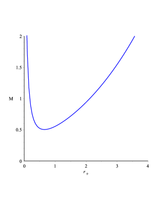
(a) $\eta=0.5,l=5.263,l=0.5$

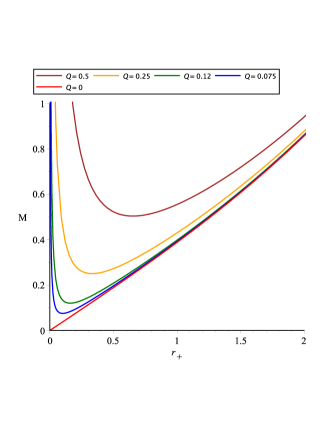
(b) $\eta=0.5,l=5.263$

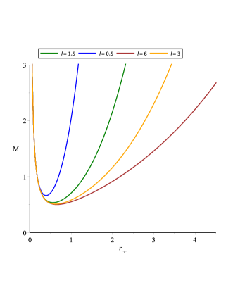
(c) $\eta=0.5,Q=0.5$

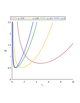
(d) $Q=0.5,l=5.263$

Figure 1: Variations of mass in terms of horizon radius $r_{+}$.

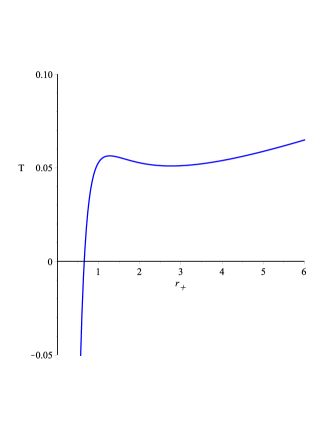
(a) $\eta=0.5,l=5.263,Q=0.5$

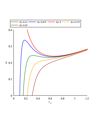
(b) $\eta=0.5,Q=0.075$

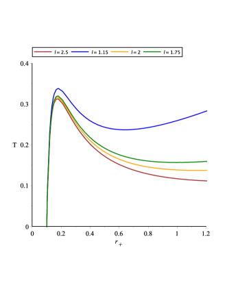
(c) $\eta=0.5,Q=0.075$

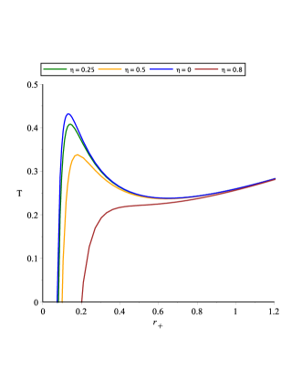
(d) $Q=0.075,l=1.15$

Figure 2: Variations of temperature in terms of horizon radius $r_{+}$.

The behavior of mass for different values of $Q$, $l$ and $\eta$, is shown in Fig. 1. It can be seen from Fig. 1(a), the mass of this black hole, has one minimum point $r_{+}=r_{m}$, in which the value of it, for $Q=0.5$, $l=5.263$ and $\eta=0.5$, is equal to 0.651. Moreover, from Fig. 1 (b)-(d), it is clear that by increasing the value of $Q$, $l$ and $\eta$, the minimum point can be occur at different location.

Also, the behavior of temperature for different values of $Q$, $l$ and $\eta$, is demonstrated in Fig. 2. It can be observed from Fig. 2(a), the plot of the temperature is in the negative region at a particular range of $r_{+}(r_{+}<r_{m})$, then it reaches to zero at $r_{+}=r_{m}$. Fig. 2(a)-(d), shows that for $r_{+}>r_{m}$, the temperature will be positive and increases to a maximum point. After that it starts decreasing with higher $r_{+}$ and then again starts increases gradually. A comparative analysis of these plots reflects that as long as the values of $Q$, $l$ and $\eta$ increases, the peak value of temperature becomes smaller.

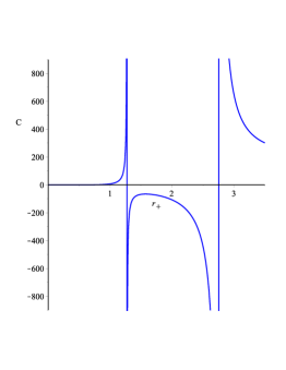
(a) $Q=0.5,\eta=0.5,l=5.263$

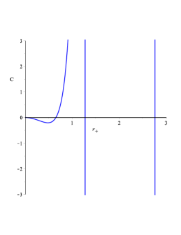
(b) closeup of figure (a)

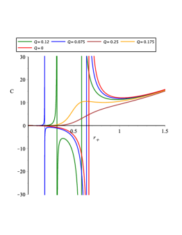
(c) $\eta=0.5,l=1.15$

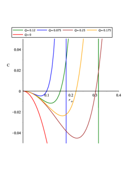
(d) closeup of figure (b)

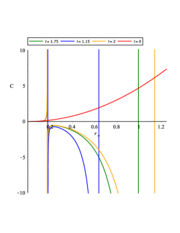
(e) $\eta=0.5,Q=0.075$

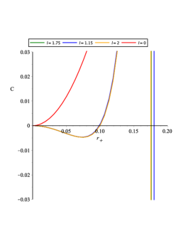
(f) closeup of figure (e)

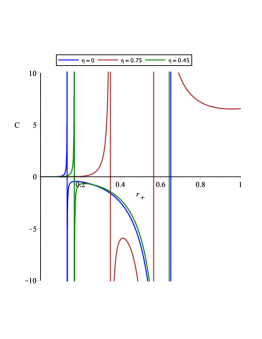
(g) $Q=0.075,l=1.15$

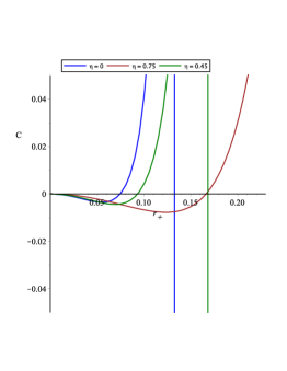
(h) closeup of figure (g)

Figure 3: Variations of the heat capacity in terms of horizon radius $r_{+}$.

In addition, the behavior of heat capacity for different values of $Q$, $l$ and $\eta$, is depicted in Fig. 3. Note that, the root of heat capacity ($C=T=0$) is showing a boundary line between non-physical ($T<0$) and physical ($T>0$) black holes and it call a physical limitation point [25]. Sign of the heat capacity changes in this physical limitation point. As we can see from Fig. 3 (a), (b), for $Q=0.5$, $l=5.263$ and $\eta=0.5$, heat capacity has one zero point at $r_{+}=r_{1}=0.651$, which corresponds to a physical limitation point, and also this corresponds to $T=0$ ($r_{+}=r_{m}$). Moreover it has two divergence points at $r_{+}=r_{2}=1.27$ and $r_{+}=r_{3}=2.76$, which demonstrate phase transition critical points of a charged AdS black hole with a global monopole. In other words, the heat capacity is negative at $r_{+}<r_{1}$, which means that the black hole system is unstable. Then, at $r_{1}<r_{+}<r_{2}$, heat capacity is positive, which means that it is in stable phase. Afterward, at $r_{2}<r_{+}<r_{3}$, it falls in to a negative region (unstable phase) and, at $r_{+}>r_{3}$, it becomes stable. Moreover, from Fig. 3 (c)-(h), by increasing the value of $Q$, $l$ and $\eta$, the phase transitions occur at different locations.

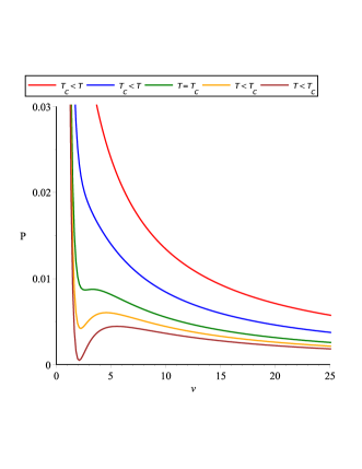
(a) $\eta=0$

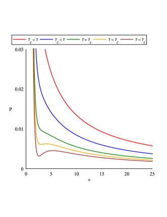
(b) $\eta=0.5$

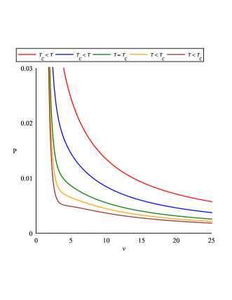
(c) $\eta=0.75$

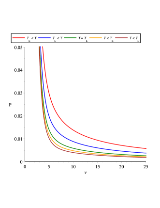
(d) $\eta=0.97$

Figure 4: $P$ - $v$ diagram of a charged AdS black hole with a global monopole in extended phase space for $Q=0.85$, $l=1.5$ and different values of $\eta$.

Fig. 4 shows $P-v$ diagrams of the charged AdS black hole with a global monopole, in extended phase space for $Q=0.85$, $l=1.5$ and different values of $\eta$. Under a critical temperature ($T_{c}$), a critical behavior appears and with larger values of $\eta$, this behavior reduces. Also, with larger values of $\eta$, $v_{c}$ increases while $T_{c}$ and $P_{c}$ decrease.

4 Thermodynamic geometry

In this section, we study the geometric structure of Weinhold, Ruppiner, Quevedo and HPEM formalisms, and investigate phase transition of a charged AdS black hole with a global monopole. The Weinhold geometry is specified in mass representation as [19]

$$g^{W}_{ij}=\partial_{i}\partial_{j}M(S,l,Q),$$ (4.1)

and the line element for a charged AdS black hole with a global monopole is given by [30]

$$ds^{2}_{W} = M_{SS}dS^{2}+M_{ll}dl^{2}+M_{QQ}dQ^{2}+2M_{Sl}dSdl+2M_{SQ}dSdQ+2M_{lQ}dldQ.$$ (4.2)

Therefore the relevant matrix is

$$g^{W}=\begin{bmatrix}M_{SS}&M_{Sl}&M_{SQ}\\ M_{lS}&M_{ll}&0\\ M_{QS}&0&M_{QQ}\end{bmatrix}.$$ (4.3)

So, the curvature scalar of the Weinhold metric ($R^{W}$) is given by

$$R^{W}=\frac{l^{2}~{}\pi^{3/2}~{}S^{1/2}~{}\left(\pi^{2}~{}Q^{2}~{}l^{2}-\pi~{}S~{}\eta^{2}~{}l^{2}+\pi~{}S~{}l^{2}+9~{}S^{2}\right)\left({1-\eta^{2}}\right)^{1/2}}{\left(\pi^{2}~{}Q^{2}~{}l^{2}+\pi~{}S~{}\eta^{2}~{}l^{2}-\pi~{}S~{}l^{2}-3~{}S^{2}\right)^{2}~{}}.$$ (4.4)

The other formalism that we consider here is the Ruppiner metric. The Ruppiner metric in the thermodynamic system is introduced as [18, 31, 32]

$$ds^{2}_{R}=\frac{1}{T}ds^{2}_{W},$$ (4.5)

and the relevant matrix is

$$g^{R}=\left(\frac{4{l}^{2}{\pi}^{3/2}S\sqrt{-{{S({\eta}^{2}-1)}{}}}}{{\pi}^{2}{Q}^{2}{l}^{2}+\pi\,S{\eta}^{2}{l}^{2}-\pi\,S{l}^{2}-3\,{S}^{2}}\right)\begin{bmatrix}M_{SS}&M_{Sl}&M_{SQ}\\ M_{lS}&M_{ll}&0\\ M_{QS}&0&M_{QQ}\end{bmatrix}.$$ (4.6)

Therefore, the curvature scalar of the Ruppiner formalism is calculated by

$$R^{Rup}=-\frac{\pi\,{l}^{2}\left(2\,\pi\,{Q}^{2}+S{\eta}^{2}-S\right)}{\left({\pi}^{2}{Q}^{2}{l}^{2}+\pi\,S{\eta}^{2}{l}^{2}-\pi\,S{l}^{2}-3\,{S}^{2}\right)\\ \mbox{}S}.$$ (4.7)

The resulting curvature scalar of Weinhold and Ruppiner metrics are plotted, in terms of horizon radius $r_{+}$, to investigate thermodynamic phase transition (see Fig. 5).

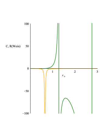
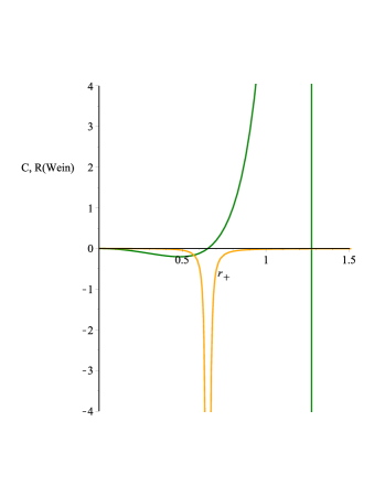
(a) Closeup of figure (a)

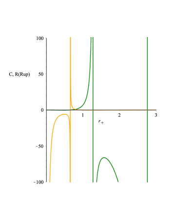
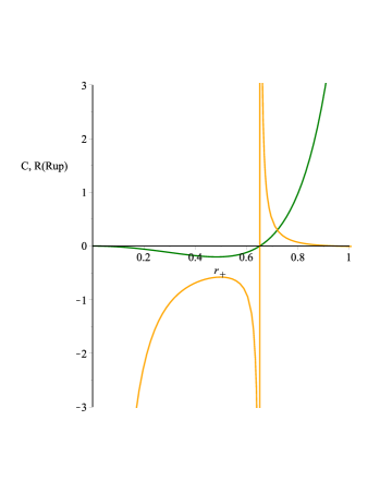
(b) Closeup of figure (c)

Figure 5: Curvature scalar variation of Weinhold and Ruppeiner metrics (orange line), and also heat capacity variation (Green line), in terms of horizon radius $r_{+}$ for $Q=0.5$, $l=5.263$, $\eta=0.5$.

As already noted in Sec. 3, from Fig. 3, that heat capacity has one zero point at $r_{+}=0.651$, which represents a physical limitation point and has two divergence points at $r_{+}=1.27$ and $r_{+}=2.76$, which demonstrate phase transition critical points of a charged AdS black hole with a global monoploe [25]. Also, from Fig. 5, we see that the curvature scalar of Weinhold and Ruppeiner metrics has one singular point at $r_{+}=0.651$, which coincides only with zero point of the heat capacity (physical limitation point).

Now, we use the Quevedo and HPEM metrics to investigate the thermodynamic properties of a charged AdS black hole with a global monopole. For Quevedo formalism, the general form of the metric is given by  [33]:

$$g=\left(E^{c}\frac{\partial\Phi}{\partial E^{c}}\right)\left(\eta_{ab}\delta^{bc}\frac{\partial^{2}\Phi}{\partial E^{c}\partial E^{d}}dE^{a}dE^{d}\right),$$ (4.8)

where

$$\frac{\partial\Phi}{\partial E^{c}}=\delta_{cb}I^{b}.$$ (4.9)

Here, $\Phi$ is the thermodynamic potential, $E^{a}$ and $I^{b}$ are the extensive and intensive thermodynamic variables, respectively. Moreover, the generalized HPEM metric with $n$ extensive variables ($n\geq 2$) is given by [15, 23, 24, 25]

$$ds_{HPEM}^{2}=\dfrac{SM_{S}}{\left(\prod_{i=2}^{n}\frac{\partial^{2}M}{\partial\chi_{i}^{2}}\right)^{3}}\left(-M_{SS}dS^{2}+\sum_{i=2}^{n}\left(\frac{\partial^{2}M}{\partial\chi_{i}^{2}}\right)d\chi_{i}^{2}\right),$$ (4.10)

in which, $\chi_{i}(\chi_{i}\neq S)$, $M_{S}=\frac{\partial M}{\partial S}$ and $M_{SS}=\frac{\partial^{2}M}{\partial S^{2}}$ are extensive parameters.

The Quevedo and HPEM metrics can be written, collectively, as [15, 23, 24, 25]

$$ds^{2}=\begin{cases}(SM_{S}+lM_{l}+QM_{Q})(-M_{SS}dS^{2}+M_{ll}dl^{2}+M_{QQ}dQ^{2})&$Quevedo Case I $\\ SM_{S}(-M_{SS}dS^{2}+M_{ll}dl^{2}+M_{QQ}dQ^{2})&$Quevedo Case II $\\ \dfrac{SM_{S}}{\left(\frac{\partial^{2}M}{\partial l^{2}}\frac{\partial^{2}M}{\partial Q^{2}}\right)^{3}}\left(-M_{SS}dS^{2}+M_{ll}dl^{2}+M_{QQ}dQ^{2}\right)&$ HPEM $.\end{cases}$$ (4.11)

Meanwhile, these metrics have following denominator for their Ricci scalars [15, 24, 25]:

$$\mbox{denom}(R)=\begin{cases}2M_{SS}^{2}M_{ll}^{2}M_{QQ}^{2}(SM_{S}+lM_{l}+QM_{Q})^{3}&$Quevedo Case I $\\ 2S^{3}M_{SS}^{2}M_{ll}^{2}M_{QQ}^{2}M_{S}^{3}&$Quevedo Case II $\\ 2S^{3}M_{SS}^{2}M_{S}^{3}&$ HPEM $.\end{cases}$$ (4.12)

The above mentioned equations are solved and plotted in terms of horizon radius $r_{+}$ (see Fig. 6).

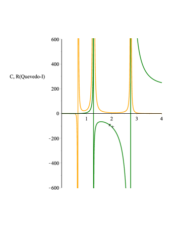
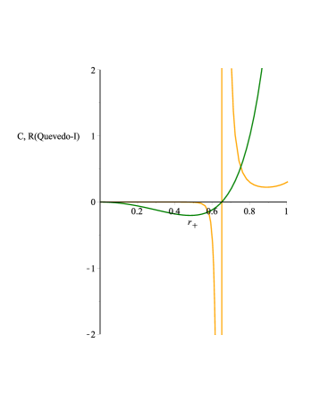
(a) Closeup of figure (a)

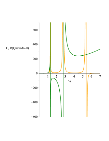
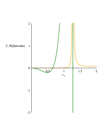
(b) Closeup of figure (c)

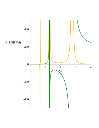
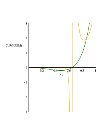
(c) Closeup of figure (e)

Figure 6: Curvature scalar variation of Quevedo and HPEM metrics (orange line) and also heat capacity variation (Green line), in terms of horizon radius $r_{+}$ for $Q=0.5$ and $\eta=0.5$, $l=5.263$ .

Moreover, it can be observed from Fig. 6(a),(b) that the curvature scalar of Quevedo (case-I) metric has three singular points at $r_{+}=0.651$, $r_{+}=1.27$ and $r_{+}=2.76$, which coincide with zero point (physical limitation point) and divergence points (transition critical points) of heat capacity, respectively.

In addition, Fig. 6(c),(d) shows that the curvature scalar of Quevedo (case-II) metric has three singular points at $r_{+}=1.27$, $r_{+}=2.76$ and $r_{+}=5.39$, in which two of them only coincide with divergences points (transition critical points) of heat capacity and no singular point coincides with zero point of heat capacity.

Furthermore, in case of HPEM metric, as shown in Fig. 6(e),(f), the divergence points of the Ricci scalar (i.e. $r_{+}=0.651$, $r_{+}=1.27$ and $r_{+}=2.76$) are coincident with zero point (physical limitation point) and divergence points (transition critical points) of heat capacity, respectively. So, the divergence points of the Ricci scalar of HPEM and Quevedo (case-I) metrics coincide with both types of phase transitions of the heat capacity. Therefore, it can be claimed that one can extract more information from HPEM and Quevedo cases as compared with Weinhold and Ruppeiner metrics.

5 Conclusions

In order to discuss phase transition of a charged AdS black hole with a global monopole through geometrical thermodynamics, we have first written metric for a charged AdS black hole with global monopole. We have shed light on the Hawking temperature, specific heat and electric potential for the system. Here, we have derived critical parameters also for this black hole. We have studied the behavior of temperature in terms of horizon radius for different values of charge, AdS radius and monopole parameter and observed that Hawking temperature first increases to a maximum point and then starts falling as horizon radius increases. Finally, after reaching a certain value of event horizon radius, the Hawking temperature only increases with horizon radius.

Moreover, we have plotted heat capacity with respect to horizon radius for different values of charge, AdS radius and monopole parameter. Interestingly, we have found that for certain values of these parameters, heat capacity has one zero point describing a physical limitation point. Also, heat capacity has two divergence points, which describe phase transition critical points of a charged AdS black hole with a global monopole. We have plotted pressure-volume curve also for the charged AdS black hole with a global monopole for the specific values of the parameters. Below critical temperature, a critical behavior has been observed which changes with larger values of energy scale. Remarkably, for larger values of the energy scale (monopole parameter), in contrast to critical temperature and critical pressure, only critical volume increases.

Subsequently, we have provided the geometric structure of Weinhold, Ruppiner, Quevedo and HPEM formalisms in order to investigate phase transition of a charged AdS black hole with a global monopole. In this regard, we have computed first the curvature scalar of Weinhold and Ruppeiner metrics. We have plotted these scalar curvature with horizon radius. These plots suggested that the curvature scalar of Weinhold and Ruppeiner metrics has one singular point, which coincides only with zero point of the heat capacity.

The Quevedo and HPEM formalisms are also implemented to investigate the thermodynamic properties of a charged AdS black hole with a global monopole. We have observed that the curvature scalar of Quevedo metric (case-I) has three singular points, which coincide with zero point (physical limitation point) and divergence points (transition critical points) of heat capacity, respectively. However, in case of curvature scalar of Quevedo (case-II) metric, there exist three singular points; two of them only coincide with divergences points (transition critical points) of heat capacity and no point coincides with zero point of heat capacity. In case of HPEM metric, The curvature scalar exhibits divergence points which are coincident with zero point (physical limitation point) and divergence points (transition critical points) of heat capacity, respectively. Here, we concluded that the divergence points of the Ricci scalar of HPEM and Quevedo (case-I) metrics coincide with both types of phase transitions of the heat capacity. These analysis suggest that one can get more information about the phase transition for the charged AdS black hole with a global monopole from HPEM and Quevedo methods in comparison to the Weinhold and Ruppeiner cases.

References

- [1] J. D. Bekenstein, Phys. Rev. D 7, 2333 (1973).
- [2] S. W. Hawking, Commun. Math. Phys. 43 (1975) 199.
- [3] S. W. Hawking and D. N. Page, Commun. Math. Phys. 87 (1983) 577.
- [4] D. N. Page, New J. Phys. 7 (2005) 203.
- [5] T. W. B. Kibble, J. Phys. A9 (1976) 1387.
- [6] A. Vilenkin, Phys. Rept. 121 (1985) 263.
- [7] M. Barriola and A. Vilenkin, Phys. Rev. Lett. 63, 341 (1989).
- [8] X. Shi and X.-z. Li, Class. Quant. Grav. 8 (1991) 761.
- [9] A. Banerjee, S. Chatterjee and A. Sen, Class. Quant. Grav. 13 (1999) 3141.
- [10] S. Chen and J. Jing, Class. Quant. Grav. 30 (2013) 175012.
- [11] K. Jusufi, M. C. Werner, A. Banerjee and A. vgn, Phys. Rev. D95 (2017) 104012.
- [12] M. Appels, R. Gregory and D. Kubiznak, Phys. Rev. Lett. 117 (2016) 131303.
- [13] M. Appels, R. Gregory and D. Kubiznak, JHEP 05 (2017) 116.
- [14] S. Chen, L. Wang, C. Ding and J. Jing, Nucl. Phys. B836 (2010) 222.
- [15] S. Soroushfar, R. Saffari and S. Upadhyay, Gen. Rel. Grav. 51, 130 (2019).
- [16] S. Upadhyay, S. Soroushfar and R. Saffari, arXiv:1801.09574.
- [17] B. Pourhassan and S. Upadhyay, arXiv:1910.11698.
- [18] G. Ruppeiner, Phys. Rev. A 20, 1608 (1979).
- [19] F. Weinhold, J. Chem. Phys 63, 2479 (1975).
- [20] P. Salamon, E. Ihrig, R. S. Berry, J. Math. Phys. 24, 2515 (1983).
- [21] R. Mrugala, J. D. Nulton, J. C. Schon, P. Salamon, Phys. Rev. A 41, 3156 (1990).
- [22] H. Quevedo, J. Math. Phys. 48 (2007) 013506.
- [23] S. H. Hendi, S. Panahiyan, B. Eslam Panah and M. Momennia, Eur. Phys. J. C 75, no. 10, 507 (2015).
- [24] S. H. Hendi, A. Sheykhi, S. Panahiyan and B. Eslam Panah, Phys. Rev. D 92, 064028 (2015).
- [25] B. Eslam Panah, Phys. Lett. B 787, 45 (2018).
- [26] G.-Ming Deng, J. Fan, X. Li and Y.-Chang Huang, Int. J. Mod. Phys. A 33, 1850022 (2018).
- [27] A. N. Kumara, C. L. A. Rizwan, D. Vaid and K. M. Ajith, arXiv:1906.11550 [gr-qc].
- [28] A. Rizwan C.L., N. Kumara A., D. Vaid and K. M. Ajith, Int. J. Mod. Phys. A 33, 1850210 (2019).
- [29] S. Gunasekaran, R. B. Mann and D. Kubiznak, JHEP 1211, 110 (2012).
- [30] S. Soroushfar, R. Saffari and N. Kamvar, Eur. Phys. J. C 76, 476 (2016).
- [31] P. Salamon, J. D. Nulton and E. Ihrig, J. Chem. Phys, 80,436 (1984).
- [32] R. Mrugala, Physica. A (Amsterdam), 125, 631 (1984).
- [33] H. Quevedo,J. Math. Phys. 48 (2007) 013506.