A Kogbetliantz-type algorithm for the hyperbolic SVD

Abstract

In this paper a two-sided, parallel Kogbetliantz-type algorithm for the hyperbolic singular value decomposition (HSVD) of real and complex square matrices is developed, with a single assumption that the input matrix, of order $n$, admits such a decomposition into the product of a unitary, a non-negative diagonal, and a $J$-unitary matrix, where $J$ is a given diagonal matrix of positive and negative signs. When $J=\pm I$, the proposed algorithm computes the ordinary SVD.

The paper’s most important contribution—a derivation of formulas for the HSVD of $2\times 2$ matrices—is presented first, followed by the details of their implementation in floating-point arithmetic. Next, the effects of the hyperbolic transformations on the columns of the iteration matrix are discussed. These effects then guide a redesign of the dynamic pivot ordering, being already a well-established pivot strategy for the ordinary Kogbetliantz algorithm, for the general, $n\times n$ HSVD. A heuristic but sound convergence criterion is then proposed, which contributes to high accuracy demonstrated in the numerical testing results. Such a $J$-Kogbetliantz algorithm as presented here is intrinsically slow, but is nevertheless usable for matrices of small orders.

1 Introduction

The Kogbetliantz algorithm Kogbetliantz-55 is the oldest effective method discovered that computes the singular value decomposition (SVD) of a square matrix $G$ as $G=U\Sigma V^{\ast}$, where $U$ and $V$ are unitary matrices, while $\Sigma$ is a diagonal matrix with the non-negative diagonal elements, called the singular values, that are usually ordered non-increasingly, i.e., $\Sigma=\mathop{\mathrm{diag}}(\sigma_{1},\ldots,\sigma_{n})$ and $\sigma_{k}\geq\sigma_{\ell}\geq 0$, for $1\leq k<\ell\leq n$, with $n$ being the matrix order of $G$, $U$, $\Sigma$, and $V$.

In this paper a Kogbetliantz-type algorithm for the hyperbolic singular value decomposition Onn-Steinhardt-Bojanczyk-91 (the HSVD in short) is developed and called the $J$-Kogbetliantz algorithm in the following. Since the Kogbetliantz-type algorithms operate only on square matrices, Definition 1 of the HSVD is restricted to such a case.

Definition 1

Let $J$ and $G$ be two square matrices of order $n$, such that $J$ is a diagonal matrix of signs, $J=\mathop{\mathrm{diag}}(\pm 1)$, and $G$ is a matrix over $\mathbb{F}\in\{\mathbb{R},\mathbb{C}\}$ with $\mathop{\mathrm{rank}}(GJG^{\ast})=\mathop{\mathrm{rank}}(G)$. A decomposition of $G$,

$$G=U\Sigma V^{-1},$$

such that $U$ is a unitary matrix over $\mathbb{F}$, $V$ is a $J$-unitary matrix over $\mathbb{F}$ with respect to $J$ (i.e., $V^{\ast}JV=J$, so $V$ is hypernormal in the terminology of Bojanczyk-Onn-Steinhardt-93 ), and $\Sigma$ is a real diagonal matrix with a non-negative diagonal, is called the hyperbolic singular value decomposition of $G$. The diagonal elements of $\Sigma$ are called the hyperbolic singular values of $G$, which are assumed to be ordered non-increasingly (non-decreasingly) in any, not necessarily contiguous, range of diagonal elements of $\Sigma$ for which the corresponding range of diagonal elements of $J$ contains only positive (negative) signs.

When $J=\pm I_{n}$ the HSVD becomes the ordinary SVD, with $V$ unitary, and the $J$-Kogbetliantz algorithm reduces to the ordinary Kogbetliantz algorithm for the SVD.

In Definition 1 the assumption that $\mathop{\mathrm{rank}}(GJG^{\ast})=\mathop{\mathrm{rank}}(G)$ ensures Zha-96 that the HSVD of $G$ exists, with a diagonal $\Sigma$. If the assumption does not hold, or if $G$ is rectangular, for the $J$-Kogbetliantz algorithm $G$ should be preprocessed by, e.g., the $J$-URV factorization SingerSanja-06 ; Singer-DiNapoli-Novakovic-Caklovic-20 to a square matrix $G_{0}$ of order $n_{0}\leq n$, such that $\mathop{\mathrm{rank}}(G_{0}J_{0}G_{0}^{\ast})=\mathop{\mathrm{rank}}(G_{0})$, i.e., $G=U_{0}^{\ast}\widetilde{G}_{0}V_{0}$, where $U_{0}$ is unitary, $V_{0}$ is $J$-unitary, $J_{0}=\mathop{\mathrm{diag}}(\pm 1)$ is of order $n_{0}$, and $G_{0}=\widetilde{G}_{0}(1:n_{0},1:n_{0})$. Otherwise, let $n_{0}=n$, $G_{0}=G$, $V_{0}=U_{0}=I_{n}$, and $J_{0}=J$.

Besides an obvious application as the main part of a method for solving a Hermitian indefinite eigenproblem Singer-et-al-12a ; Singer-et-al-12b , the HSVD has also been used in various signal processing applications Onn-Steinhardt-Bojanczyk-91 , and recently in a modified approach to the Kalman filtering, especially in the ill-conditioned case Kulikov-Kulikova-20 ; Kulikova-19a ; Kulikova-19b . The HSVD can be efficiently and accurately computed by the one-sided blocked Jacobi-type algorithms Hari-SingerSanja-SingerSasa-10 ; Hari-SingerSanja-SingerSasa-14 , even on the massively parallel architectures Novakovic-15 . A two-sided, Kogbetliantz-type method proposed here is not intended to outperform the existing one-sided HSVD algorithms. Instead, it is meant to showcase the tools (e.g., a careful dynamic parallel ordering and a sound convergence criterion) designed to cope with the perils of non-unitary transformations, that empirically happen to be a greater risk for numerical stability of the two-sided methods—here, for the hyperbolic, but possibly also applicable to the more general, orthosymmetric Mackey-Mackey-Tisseur-05 SVD—than for that of the one-sided algorithms.

The ordinary Kogbetliantz algorithm usually transforms an upper triangular matrix $R$ (see, e.g., Hari-Veselic-87 ), resulting from the preprocessing of $G$ by the QR factorization, in order to simplify the transformations and lower their number. If a particular cyclic pivot ordering is applied, at the end of the first cycle a lower triangular matrix is obtained, while after the subsequent cycle the iteration matrix becomes upper triangular again. Unfortunately, a simple generalization of the Kogbetliantz algorithm to a hyperbolic one (by introducing the hyperbolic transformations but leaving the pivot strategy intact) can fail, since even a single hyperbolic transformation from the right, with a sufficiently high condition number, can cause an excessive growth of the off-diagonal elements of the iteration matrix and ruin the convergence of the algorithm. A different, dynamic (data-dependent) pivot strategy is therefore needed to keep the sometimes unavoidable growth of the off-diagonal norm in check. As a consequence, the iteration matrix cannot be assumed to have or retain any particular structure.

The $J$-Kogbetliantz algorithm computes the HSVD of $G_{0}$ in a sequence of transformations, infinite in general but cut off to a finite leading part when computing in machine precision and a convergence criterion is met, as

$$U^{\ast}G_{0}V\approx\Sigma,\quad U^{\ast}=U_{N}^{\ast}U_{N-1}^{\ast}\cdots U_{1}^{\ast},\quad V=V_{1}V_{2}\cdots V_{N},$$

where, for each $k$, $1\leq k\leq N$, $U_{k}^{\ast}$ and $V_{k}$ are the embeddings of the $2\times 2$ transformations $\widehat{U}_{k}^{\ast}$ and $\widehat{V}_{k}$, respectively, into $I_{n_{0}}$, that are applied to the iteration matrix $G_{k-1}$, forming a sequence of the iteration matrices

$$G_{1},G_{2},\ldots,G_{N}\approx\Sigma,$$

where $G_{k}=U_{k}^{\ast}G_{k-1}V_{k}$. If $G_{0}$ is already in the form required of $\Sigma$, then $V=U=I_{n_{0}}$, $\Sigma=G_{0}$, and no transformations take place. Else, $U_{k}^{\ast}$ is unitary (orthogonal in the real case), while $V_{k}$ is $J_{0}$-unitary ($J_{0}$-orthogonal in the real case). Each $\widehat{U}_{k}^{\ast}$ is unitary (orthogonal), and $\widehat{V}_{k}$ is $\widehat{J}_{k}$-unitary ($\widehat{J}_{k}$-orthogonal), where $\widehat{J}_{k}=\mathop{\mathrm{diag}}(J_{0}(p_{k},p_{k}),J_{0}(q_{k},q_{k}))$ for the $k$th pivot index pair $(p_{k},q_{k})$, $1\leq p_{k}<q_{k}\leq n_{0}$. The decomposition is finalized by forming $U=(U^{\ast})^{\ast}=U_{1}U_{2}\cdots U_{N}$, while by multiplying $V^{\ast}J_{0}V=J_{0}$ from the left by $J_{0}$, and noting that $J_{0}^{2}=I_{n_{0}}$, it follows that $V^{-1}=J_{0}V^{\ast}J_{0}$.

In the $k$th step the elements $(1,1)$, $(2,1)$, $(1,2)$, and $(2,2)$ of $\widehat{U}_{k}^{\ast}$ (and $\widehat{V}_{k}$) are embedded into $U_{k}^{\ast}$ (and $V_{k}$) at the pivot positions $(p_{k},p_{k})$, $(q_{k},p_{k})$, $(p_{k},q_{k})$, and $(q_{k},q_{k})$, respectively, where the pivot indices are chosen such that for the pivot matrix $\widehat{G}_{k-1}$,

$$\widehat{G}_{k-1}=\begin{bmatrix}G_{k-1}(p_{k},p_{k})&G_{k-1}(p_{k},q_{k})\\ G_{k-1}(q_{k},p_{k})&G_{k-1}(q_{k},q_{k})\end{bmatrix},$$ (1)

holds at least one of

$$\widehat{G}_{k-1}(2,1)\neq 0,\quad\widehat{G}_{k-1}(1,2)\neq 0,\quad\widehat{G}_{k-1}(1,1)\notin\mathbb{R}_{0}^{+},\quad\widehat{G}_{k-1}(2,2)\notin\mathbb{R}_{0}^{+}.$$

When $\widehat{J}_{k}(1,1)=\widehat{J}_{k}(2,2)$ (such a case is called trigonometric in the following, while the other case is called hyperbolic), $\widehat{G}_{k-1}$ is also a transformation candidate if it is diagonal, with the non-negative diagonal elements such that $\widehat{G}_{k-1}(1,1)<\widehat{G}_{k-1}(2,2)$ if $\widehat{J}_{k}=I_{2}$, or $\widehat{G}_{k-1}(1,1)>\widehat{G}_{k-1}(2,2)$ if $\widehat{J}_{k}=-I_{2}{}$. This is summarized in Definition 2.

Definition 2

In a step $k\geq 1$, let $p_{k}$ and $q_{k}$, $1\leq p_{k}<q_{k}\leq n_{0}$, be such indices for which $\widehat{G}_{k-1}$ from (1) does not have a form required of a matrix of hyperbolic singular values, as specified in Definition 1. Then, $\widehat{G}_{k-1}$ is called a transformation candidate or a pivot (sub)matrix. If such indices do not exist, there are no transformation candidates in the $k$th step. If more than one index pair satisfies the defining condition, one pivot index pair is selected according to the chosen pivot strategy.

If the step index is omitted, then for the pivot index pair $(p,q)$ the transformation matrices ($\widehat{U}^{\ast}$ and $\widehat{V}$), the pivot matrix ($\widehat{G}$), and the corresponding matrices of signs ($\widehat{J}$) and hyperbolic singular values ($\widehat{\Sigma}$) can be written as

$$\widehat{U}^{\ast}=\begin{bmatrix}\bar{u}_{pp}&\bar{u}_{qp}\\ \bar{u}_{pq}&\bar{u}_{qq}\end{bmatrix}\!,\;\widehat{V}=\begin{bmatrix}v_{pp}&v_{pq}\\ v_{qp}&v_{qq}\end{bmatrix}\!,\;\widehat{G}=\begin{bmatrix}g_{pp}&g_{pq}\\ g_{qp}&g_{qq}\end{bmatrix}\!,\;\widehat{J}=\begin{bmatrix}j_{pp}&0\\ 0&j_{qq}\end{bmatrix}\!;\;\widehat{\Sigma}=\begin{bmatrix}\sigma_{pp}&0\\ 0&\sigma_{qq}\end{bmatrix}\!.$$

With $\widehat{G}$ given, $\widehat{U}^{\ast}$ and $\widehat{V}$ are sought for, such that $\widehat{U}^{\ast}\widehat{G}\widehat{V}=\widehat{\Sigma}$, with $\sigma_{pp}$ and $\sigma_{qq}$ being the hyperbolic singular values of $\widehat{G}$, and $\widehat{V}^{\ast}\widehat{J}\widehat{V}=\widehat{J}$.

If there are no transformation candidates in the $k$th step, or if the convergence criterion is satisfied, the algorithm stops successfully, with (an approximation of) the HSVD of $G$ found. Otherwise, $\widehat{U}_{k}^{\ast}$ and $\widehat{V}_{k}$ are computed for one, suitably chosen transformation candidate of $G_{k-1}$, and applied to the pivot rows $p_{k}$ and $q_{k}$ from the left ($\widehat{U}_{k}^{\ast}$) and the pivot columns $p_{k}$ and $q_{k}$ from the right ($\widehat{V}_{k}$), in that order for determinacy, to form $G_{k}$. The process is then repeated in the step $k+1$.

Note that several, but at most $\lfloor n_{0}/2\rfloor$ successive steps can be grouped to form a multi-step $\mathbf{k}$, where $0\leq|\mathbf{k}|\leq\lfloor n_{0}/2\rfloor$ is the chosen length of $\mathbf{k}$, if and only if $\{p_{k},q_{k}\}\cap\{p_{l},q_{l}\}=\emptyset$ for all $k\neq l$ such that $\{k,l\}\subseteq\mathbf{k}$, i.e., all basic steps within a multi-step can be performed in parallel (with $t\geq 1$ parallel tasks at hand). The number of basic steps may vary from one multi-step to another if, e.g., not enough transformation candidates are available, and may reach zero when no further transformations are possible. With $n_{0}=6$, e.g., the multi-step $\mathbf{1}$ might be $\{1,2,3\}$, $\mathbf{2}$ might be $\{4,5\}$, $\mathbf{3}$ might be $\{6,7,8\}$, continuing until some $\mathbf{N}$ at which the algorithm halts.

The parallel application of the $2\times 2$ transformations has to take into account that all transformations from one side (e.g., the row transformations from the left) have to precede any transformation from the other side (e.g., the column transformations from the right). However, all transformations from the same side can proceed concurrently, and the choice of the first side to be transformed is arbitrary.

To fully describe the $J$-Kogbetliantz algorithm, it therefore suffices to specify:

1. a method for computing the HSVD of the pivot matrices of order two,

2. the details of performing the row and the column transformations,

3. a pivot strategy that selects the transformation candidate(s) in a (multi-)step, and

4. a convergence criterion that halts the execution.

The above list guides the organization of this paper as follows. The first item is covered in section 2, the second one in section 3, the third one in section 4, and the last one in section 5, containing an overview of the algorithm. The numerical testing results are summarized in section 6, and the paper is concluded with some remarks on the future work in section 7. Appendix A contains several technical proofs.

2 Computing the HSVD of matrices of order two

In the ordinary Kogbetliantz algorithm it is preferred that the pivot matrices throughout the process remain (upper or lower) triangular Charlier-Vanbegin-VanDooren-87 ; Hari-Veselic-87 under a cyclic pivot strategy: a serial (e.g., the row or the column cyclic, with $G_{0}$ triangular) or a parallel one (e.g., the modulus strategy, with $G_{0}$ preprocessed into the butterfly form Hari-Zadelj-Martic-07 )—a fact relied upon for a simple and accurate computation of the transformation parameters Hari-Matejas-09 ; Matejas-Hari-10 ; Matejas-Hari-15 . However, the $J$-Kogbetliantz algorithm employs a strategy that has no periodic (cyclic) pattern, so no particular form of the pivot matrices can be guaranteed and no special form of $G_{0}$ is presumed. Depending on $\widehat{J}$ and its own structure, a transformation candidate $\widehat{G}$ might have to be preprocessed into a real, triangular form with non-negative elements that is suitable for a novel, numerically stable computation of the transformation matrices $\widehat{U}^{\ast}$ and $\widehat{V}$ and the hyperbolic singular values in $\widehat{\Sigma}$.

2.1 The $\widehat{J}$-UTV factorization of $\widehat{G}$

The preprocessing of $\widehat{G}$ starts with checking if $\widehat{G}$ is diagonal, because this information will affect the convergence criterion (see subsection 5.1) and can simplify an optimized implementation of the $2\times 2$ HSVD. Then, $\widehat{G}$ is transformed into a real, triangular matrix $\widehat{T}$ with non-negative elements by the $\widehat{J}$-UTV factorization that preserves the hyperbolic singular values. The $\widehat{J}$-UTV factorization is similar to the URV Stewart-92 factorization, with the form

$$\check{U}^{\ast}\widehat{G}\check{V}=\widehat{T},$$

where $\check{U}$ is unitary, $\check{V}$ is $\widehat{J}$-unitary, and $\widehat{T}$ is either upper or lower triangular with real, non-negative elements. Moreover, $\widehat{T}$ is upper triangular in the trigonometric case, and $\hat{t}_{11}^{2}\geq\hat{t}_{12}^{2}+\hat{t}_{22}^{2}$. In the hyperbolic case $\widehat{T}$ is either upper triangular, as described, or lower triangular, with $\hat{t}_{22}^{2}\geq\hat{t}_{21}^{2}+\hat{t}_{11}^{2}$, depending on whether the first or the second column of $\widehat{G}$ has a greater Frobenius norm, respectively. The $2\times 2$ $\widehat{J}$-UTV factorization always exists and is uniquely determined, as demonstrated by Algorithm 2.1, which, given $\widehat{G}$, operates on a scaled matrix $\widehat{G}_{0}=2^{s}\widehat{G}$ to avoid the possibility of floating-point overflows. Determination of $s$ is described in subsection 2.1.1, with the only assumption that all (components of) the elements of $\widehat{G}$ are finite. Assume $\arg(0)=0$ for simplicity, and let $P_{2}$ be the $2\times 2$ permutation matrix $\left[\begin{smallmatrix}0&1\\ 1&0\end{smallmatrix}\right]$. Let Boolean flags—those being only true ($\top$) or false ($\bot$)—be denoted by small caps (e.g., d, h, and c, indicating whether $\widehat{G}_{0}$ is diagonal, whether the hyperbolic or the trigonometric case is considered, and whether the columns of $\widehat{G}_{0}$ have been swapped, respectively).

if $\widehat{G}_{0}$ is diagonal then $\text{\sc d}=\top$ else $\text{\sc d}=\bot$;

  // specifically, $\text{\sc d}=\top$ if $\widehat{G}_{0}=\mathbf{0}$ if $\widehat{J}=I_{2}$ or $\widehat{J}=-I_{2}$ then $\text{\sc h}=\bot$ else $\text{\sc h}=\top$;

  // $\bot$: trigonometric, $\top$: hyperbolic case // STAGE $1$: column pivoting of $\widehat{G}_{0}$

if $\left\|\left[\begin{smallmatrix}(\widehat{G}_{0})_{11}\\ (\widehat{G}_{0})_{21}\end{smallmatrix}\right]\right\|_{F}<\left\|\left[\begin{smallmatrix}(\widehat{G}_{0})_{12}\\ (\widehat{G}_{0})_{22}\end{smallmatrix}\right]\right\|_{F}$ then $\text{\sc c}=\top$ and $\check{V}_{1}=P_{2}$ else $\text{\sc c}=\bot$ and $\check{V}_{1}=I_{2}$;

  // if $\text{\sc h}\wedge\text{\sc c}$: $\check{V}_{1}$ is not $\widehat{J}$-unitary but it is canceled by $\check{V}_{5}$ in stage $5\text{\sc l}$

$\widehat{G}_{1}=\widehat{G}_{0}\check{V}_{1}$, $\check{V}:=\check{V}_{1}$;

  // start accumulating $\check{V}$

// STAGE $2$: make the first column of $\widehat{G}_{1}$ real and non-negative

$\check{U}_{2}^{\ast}=\begin{bmatrix}e^{-\arg{(\widehat{G}_{1})_{11}}}&0\\ 0&e^{-\arg{(\widehat{G}_{1})_{21}}}\end{bmatrix}$;

  // applied to get $(\widehat{G}_{2})_{11}=|(\widehat{G}_{1})_{11}|$ & $(\widehat{G}_{2})_{21}=|(\widehat{G}_{1})_{21}|$

$\widehat{G}_{2}=\check{U}_{2}^{\ast}\widehat{G}_{1}$, $\check{U}^{\ast}:=\check{U}_{2}^{\ast}$;

  // start accumulating $\check{U}^{\ast}$

// STAGE $3$: row pivoting of $\widehat{G}_{2}$

if $(\widehat{G}_{2})_{11}<(\widehat{G}_{2})_{21}$ then $\text{\sc r}=\top$ and $\check{U}_{3}^{\ast}=P_{2}$ else $\text{\sc r}=\bot$ and $\check{U}_{3}^{\ast}=I_{2}$;

  $\widehat{G}_{3}=\check{U}_{3}^{\ast}\widehat{G}_{2}$, $\check{U}^{\ast}:=\check{U}_{3}^{\ast}\check{U}^{\ast}$;

  // $(\widehat{G}_{3})_{11}\geq(\widehat{G}_{3})_{21}\geq 0$

// STAGE $4$: the QR factorization of $\widehat{G}_{3}$

if $\neg\text{\sc d}$ then // not d implies $(\widehat{G}_{3})_{11}>0$

      $\tan\phi=(\widehat{G}_{3})_{21}/(\widehat{G}_{3})_{11}$, $\cos\phi=1/\sqrt{1+\tan^{2}\phi}$;

        // $0\leq\phi\leq\pi/4$

       $\check{U}_{4}^{\ast}=\cos\phi\begin{bmatrix}1&\tan\phi\\ -\tan\phi&1\end{bmatrix}$;

        // the Givens rotation $\check{U}_{4}^{\ast}$ is $Q^{\ast}$ in the QR

      

else // the QR factorization of a diagonal matrix is trivial

      $\check{U}_{4}^{\ast}=I_{2}$;

        // $\phi=0$

      

end if

$\widehat{G}_{4}=\check{U}_{4}^{\ast}\widehat{G}_{3}$, $\check{U}^{\ast}:=\check{U}_{4}^{\ast}$;

  // $\widehat{G}_{4}$ is upper triangular

if $\text{\sc h}\wedge\text{\sc c}$ then // this pipeline ends with $\widehat{T}$ lower triangular

      // STAGE $5\text{\sc l}$: swap the columns of $\widehat{G}_{4}$ to cancel $\check{V}_{1}$

       $\check{V}_{5}=P_{2}$, $\widehat{G}_{5}=\widehat{G}_{4}\check{V}_{5}$, $\check{V}:=I_{2}(=\check{V}\check{V}_{5})$;

        // since $P_{2}=P_{2}^{\ast}$

       // STAGE $6\text{\sc l}$: swap the rows of $\widehat{G}_{5}$

       $\check{U}_{6}^{\ast}=P_{2}$, $\widehat{G}_{6}=\check{U}_{6}^{\ast}\widehat{G}_{5}$, $\check{U}^{\ast}:=\check{U}_{6}^{\ast}\check{U}^{\ast}$;

        // $\widehat{G}_{6}$ is lower triangular

       // STAGE $7\text{\sc l}$: make $(\widehat{G}_{6})_{21}$ real and non-negative

       $\check{V}_{7}=\begin{bmatrix}e^{-\arg{(\widehat{G}_{6})_{21}}}&0\\ 0&1\end{bmatrix}$;

        // applied to get $(\widehat{G}_{7})_{21}=|(\widehat{G}_{6})_{21}|$

       $\widehat{G}_{7}=\widehat{G}_{6}\check{V}_{7}$, $\check{V}:=\check{V}_{7}$;

        // $\check{V}_{7}$ is both unitary and $\widehat{J}$-unitary

       // STAGE $8\text{\sc l}$: make $(\widehat{G}_{7})_{11}$ real and non-negative

       $\check{U}_{8}^{\ast}=\begin{bmatrix}e^{-\arg{(\widehat{G}_{7})_{11}}}&0\\ 0&1\end{bmatrix}$;

        // applied to get $(\widehat{G}_{8})_{11}=|(\widehat{G}_{7})_{11}|$

       $\widehat{G}_{8}=\check{U}_{8}^{\ast}\widehat{G}_{7}$, $\check{U}^{\ast}:=\check{U}_{8}^{\ast}\check{U}^{\ast}$;

        // $\widehat{T}=\widehat{G}_{8}$

      

else // this pipeline ends with $\widehat{T}$ upper triangular

      // STAGE $5\text{\sc u}$: make $(\widehat{G}_{4})_{12}$ real and non-negative

       $\check{V}_{5}=\begin{bmatrix}1&0\\ 0&e^{-\arg{(\widehat{G}_{4})_{12}}}\end{bmatrix}$;

        // applied to get $(\widehat{G}_{5})_{12}=|(\widehat{G}_{4})_{12}|$

       $\widehat{G}_{5}=\widehat{G}_{4}\check{V}_{5}$, $\check{V}:=\check{V}\check{V}_{5}$;

        // $\check{V}_{5}$ is both unitary and $\widehat{J}$-unitary

       // STAGE $6\text{\sc u}$: make $(\widehat{G}_{5})_{22}$ real and non-negative

       $\check{U}_{6}^{\ast}=\begin{bmatrix}1&0\\ 0&e^{-\arg{(\widehat{G}_{5})_{22}}}\end{bmatrix}$;

        // applied to get $(\widehat{G}_{6})_{22}=|(\widehat{G}_{5})_{22}|$

       $\widehat{G}_{6}=\check{U}_{6}^{\ast}\widehat{G}_{5}$, $\check{U}^{\ast}:=\check{U}_{6}^{\ast}\check{U}^{\ast}$;

        // $\widehat{T}=\widehat{G}_{6}$

      

end if

Note: All transitions $\widehat{G}_{l}\to\widehat{G}_{l+1}$ actually happen in-place by transforming the working matrix.

Algorithm 2.1 The $\widehat{J}$-UTV factorization of a complex $2\times 2$ matrix $\widehat{G}_{0}$.

When $\widehat{T}$ is upper triangular, Algorithm 2.1 is a refinement of the URV factorization, as described in detail in Novakovic-20 for the trigonometric case, where $R=\widehat{T}$ is real and non-negative, with a prescribed relation among the magnitudes of its elements. The $2\times 2$ $\widehat{J}$-UTV factorization guarantees that $\check{V}$ is both unitary and $\widehat{J}$-unitary in all cases. When $\widehat{G}$ is real, a multiplication of an element $\hat{g}$ of the working matrix by $e^{-\arg{\hat{g}}}$ amounts to a multiplication by $\mathop{\mathrm{sign}}{\hat{g}}$, without any rounding error.

In brief, Algorithm 2.1 consists of two possible pipelines, having in common the first four stages. The longer pipeline has eight, and the shorter one six stages in total.

In a stage $\mathfrak{s}\geq 1$, the working matrix and either $\check{U}^{\ast}$ or $\check{V}$ are transformed in place, either by a left multiplication by $\widehat{U}_{\mathfrak{s}}^{\ast}$, or by a right multiplication by $\widehat{V}_{\mathfrak{s}}$, respectively. The working matrix thus progresses from the state $\widehat{G}_{\mathfrak{s}-1}$ to $\widehat{G}_{\mathfrak{s}}$, until it is eventually reduced to $\widehat{T}$, at which point $\check{U}^{\ast}$ and $\check{V}$ are considered final, i.e., the $\widehat{J}$-UTV factorization is computed. Initially, $\check{U}^{\ast}$ and $\check{V}$ are set to identities, and d and h are determined.

In stage 1, if the column pivoting of $\widehat{G}_{0}$ is needed (i.e., its first column is of lower Frobenius norm than its second), c is set to $\top$ and $\check{V}_{1}$ to $P_{2}$, else they become $\bot$ and $I_{2}$, respectively. Note that $\check{V}_{1}$ is not $\widehat{J}$-unitary if h and c are $\top$, but in that case $\check{V}_{1}$ will be cancelled by $P_{2}=P_{2}^{\ast}$, with no intervening right transformations, in stage 5l.

In stage 2, the first column of $\widehat{G}_{1}$ is made real and non-negative by $\check{U}_{2}^{\ast}$, effectively setting the elements of the first column of $\widehat{G}_{2}$ to the magnitudes of those from $\widehat{G}_{1}$. Then, it is possible to compare them in stage 3. If the first is less than the second, the rows of $\widehat{G}_{2}$ are swapped by $\check{U}_{3}^{\ast}$. In stage 4 (the final one shared among the two pipelines) the QR factorization of $\widehat{G}_{3}$ is performed. If $\widehat{G}_{0}$ was diagonal, $\widehat{G}_{3}$ will come out as such from the previous stage, and the factorization is trivial. Else, the real Givens rotation $\check{U}_{4}^{\ast}$ (i.e., $Q^{\ast}$) is computed from the elements of the first column of $\widehat{G}_{3}$. Due to the row pivoting, the rotation’s angle $\phi$ lies between $0$ and $\pi/4$. Now, $R$ from the factorization, i.e., $\widehat{G}_{4}$, is upper triangular, with its second column possibly complex, while $(\widehat{G}_{4})_{11}$ is by construction real and of the largest magnitude in $\widehat{G}_{4}$.

The remaining stages of the longer pipeline, i.e., the one in which h and c are $\top$, are described first. In stage 5l $\check{V}_{1}=P_{2}$ is cancelled by $\check{V}_{5}=P_{2}$, i.e., the columns of $\widehat{G}_{4}$ are swapped to obtain $\widehat{G}_{5}$, which in stage 6l gets its rows swapped by $\check{U}_{6}^{\ast}$ to become the lower triangular $\widehat{G}_{6}$. Stage 5l is necessary to make the current $\check{V}$ $\widehat{J}$-unitary (identity) again. Stage 6l brings the working matrix into a more “familiar” (i.e., lower triangular) form. The working matrix in this pipeline remains lower triangular until the end. To emphasize that, “l” is appended to the stage identifiers. To make the working matrix real, $\check{V}_{7}$ (obviously unitary but also $\widehat{J}$-unitary, since $\check{V}_{7}^{\ast}\widehat{J}\check{V}_{7}=\widehat{J}$, where $\widehat{J}$ has two opposite signs on its diagonal) is applied to it in stage 7l, to turn $(\widehat{G}_{6})_{21}$ into its magnitude. Finally, in stage 8l, $(\widehat{G}_{7})_{11}$ is turned into its magnitude by $\check{U}_{8}^{\ast}$.

The shorter pipeline, followed when h or c are $\bot$, keeps the working matrix upper triangular, and thus the stage identifiers have “u” appended to them. Stage 5u turns $(\widehat{G}_{4})_{12}$ into its magnitude by (similarly as above, both unitary and $\widehat{J}$-unitary) $\check{V}_{5}$, while stage 6u completes the pipeline by turning $(\widehat{G}_{5})_{22}$ into its magnitude by $\widehat{U}_{6}^{\ast}$.

Figure 1 illustrates the possible progressions of a non-diagonal complex matrix $\widehat{G}_{0}$ through the stages of Algorithm 2.1 in both its pipelines (but only one pipeline is taken with any given input), and as if all optional transformations take place (the column and/or the row pivoting may not actually happen). A diagonal matrix admits a simplified procedure, evident enough for its details to be omitted here for brevity. The state of the working matrix before the operations of each stage commence is shown, while the transformation matrices are implied by the effects of a particular stage.

$$\begin{array}[]{rcccccc@{\mkern 2.45mu}c@{\mkern 2.45mu}ccccl}\widehat{G}_{0}\mkern-1.0mu=\mkern-4.0mu\begin{bmatrix}\text{\char 182}&\text{\char 184}\\ \text{\char 183}&\text{\char 185}\end{bmatrix}&\xrightarrow[\text{\sc c}]{1}&\begin{bmatrix}\text{\char 184}&\text{\char 182}\\ \text{\char 185}&\text{\char 183}\end{bmatrix}&\xrightarrow{2}&\begin{bmatrix}\text{\char 176}&\text{\char 188}\\ \text{\char 177}&\text{\char 189}\end{bmatrix}&\xrightarrow[\text{\sc r}]{3}&\begin{bmatrix}\text{\char 177}&\text{\char 189}\\ \text{\char 176}&\text{\char 188}\end{bmatrix}&\xrightarrow{4}&\begin{bmatrix}\boxdot&\text{\char 190}\\ 0&\text{\char 191}\end{bmatrix}&\xrightarrow[\text{\sc u}]{5}&\begin{bmatrix}\boxdot&\circledcirc\\ 0&\text{\char 89}\end{bmatrix}&\xrightarrow[\text{\sc u}]{6}&\begin{bmatrix}\boxdot&\circledcirc\\ 0&\circledast\end{bmatrix}\mkern-4.0mu=\mkern-1.0mu\widehat{T}\\[8.0pt] \hbox{}\hfil&\hbox{}\hfil&\hbox{}\hfil&\hbox{}\hfil&\hbox{}\hfil&\hbox{}\hfil&\hbox{}\hfil&\swarrow&\mathclap{\text{\small 5{\sc l} ($\text{\sc h}\wedge\text{\sc c}$)}}\\[-4.0pt] \mathclap{\genfrac{}{}{0.0pt}{0}{\genfrac{}{}{0.0pt}{0}{\text{\small{\sc h}: hyperbolic case}}{\text{\small{\sc c} / {\sc r}: column / row pivoting}}}{\text{\small{\sc u} / {\sc l}: upper / lower triangular}}}&\hbox{}\hfil&\hbox{}\hfil&\hbox{}\hfil&\hbox{}\hfil&\hbox{}\hfil&\begin{bmatrix}\text{\char 190}&\boxdot\\ \text{\char 191}&0\end{bmatrix}&\xrightarrow[\text{\sc l}]{6}&\begin{bmatrix}\text{\char 191}&0\\ \text{\char 190}&\boxdot\end{bmatrix}&\xrightarrow[\text{\sc l}]{7}&\begin{bmatrix}\text{\char 89}&0\\ \circledcirc&\boxdot\end{bmatrix}&\xrightarrow[\text{\sc l}]{8}&\begin{bmatrix}\circledast&0\\ \circledcirc&\boxdot\end{bmatrix}\mkern-4.0mu=\mkern-1.0mu\widehat{T}\end{array}$$

Figure 1: A schematic representation of the $\widehat{J}$-UTV factorization pipelines of a complex $2\times 2$ matrix $\widehat{G}_{0}$. The upper pipeline is followed in the trigonometric case, or in the hyperbolic case when no column pivoting was performed in stage 1, resulting in an upper triangular $\widehat{T}$ after six transformations. Otherwise, the lower pipeline is followed from stage 5 onwards, resulting in a lower triangular $\widehat{T}$ after eight transformations of the working matrix. The symbols with a black background stand for the complex elements, while those with a white background denote the real non-negative ones. The circled numbers represent the transient values, while the framed operators are reserved for the final ones, such that $\boxdot^{2}\geq\circledcirc^{2}+\circledast^{2}$.

The numerical issues of computing in the machine precision (in Fortran) are dealt with in subsection 2.1.1 for the column norms, in subsection 2.1.2 for the polar form of a complex number, and in subsection 2.1.3 for the rotation-like transformations. It is assumed that the floating-point arithmetic is not trapping on an exception, that the rounding to nearest (with tie to even) is employed, that the gradual underflow and the fused multiply-add ($\mathop{\mathtt{fma}}$) operation are available, that $\mathop{\mathtt{HYPOT}}(a,b)=\sqrt{a^{2}+b^{2}}$ intrinsic causes no undue overflow, and that $\mathop{\mathtt{HYPOT}}(a,b)=0\iff a=b=0$.

Algorithm 2.1 is conditionally reproducible, i.e., its results on any given input are bitwise identical in every floating-point environment behaving as described above and employing the same datatype, provided that the $\mathtt{HYPOT}$ intrinsic is reproducible.

2.1.1 Determination of the scaling parameter $s$

For a complex number $z$, $|z|$ can overflow in floating-point arithmetic. The magnitude of $z$ can also pose a problem, e.g., in computing of the norms of the columns of $\widehat{G}$ in stage 1 of Algorithm 2.1 for the column pivoting in the QR factorization. There,

$$\left\|\begin{bmatrix}a&b\end{bmatrix}^{T}\right\|_{F}=\sqrt{|a|^{2}+|b|^{2}}=\mathop{\mathtt{HYPOT}}(\mathop{\mathtt{HYPOT}}(\mathop{\mathrm{Re}}{a},\mathop{\mathrm{Im}}{a}),\mathop{\mathtt{HYPOT}}(\mathop{\mathrm{Re}}{b},\mathop{\mathrm{Im}}{b}))=c,$$

so it has to be ensured, by an appropriate prescaling of $\widehat{G}$, that $|a|$, $|b|$, and $c$ do not overflow. A similar concern is addressed in the xLARTG LAPACK Anderson-et-al-99 routines, but for efficiency it is advisable to avoid the overhead of function calls in the innermost computational parts. At the same time, to avoid computing with the subnormal (components of) numbers, $\widehat{G}$ could be upscaled when no overflow can occur. Therefore, to efficiently mitigate as many overflow and underflow issues as practicable, either the following prescaling of $\widehat{G}$, and the corresponding postscaling of the resulting $\widehat{\Sigma}$, should be employed, or, without any scaling needed, the entire computation of the $2\times 2$ HSVD should be performed in a floating-point datatype at least as precise as the type of (the components of) the elements of $\widehat{G}$, but with a wider exponent range (e.g., in the Intel’s 80-bit, hardware supported extended precision datatype).

Down- and up-scalings of $\widehat{G}$ can be made (almost) exact, without any loss of precision in the vast majority of cases, by decreasing, or respectively increasing, the exponents of (the components of) the elements only, i.e., by multiplying the values by $2^{s}$ with $s\in\mathbb{Z}$, leaving the significands intact (except for a subnormal value and $s<0$, when the $|s|$ lowest bits of the significand—some of which may not be zero—perish), as explained in (Novakovic-20, , subsection 2.1) and summarized here in Fortran parlance.

Let $\mathop{\eta}(a)=\mathop{\mathtt{EXPONENT}}(a)$ for a floating-point value $a$, and let $\nu=\mathop{\eta}(\Omega)$, where $\Omega=\mathop{\mathtt{HUGE}}(\mathtt{0D0})$ is the largest finite DOUBLE PRECISION value. For $a$ finite, let

$$\mathop{\chi}(a)=\nu-\mathop{\eta}(\max\{|a|,\omega\})-2$$

be a measure of how much, in terms of its exponent, $a$ has to be downscaled, or how much it can be safely upscaled. Here and in the following, $\omega$ is the smallest non-zero positive subnormal floating-point number, while $\widehat{\omega}=\mathop{\mathtt{TINY}}(\mathtt{0D0})$ is the smallest positive normal DOUBLE PRECISION value. Two sets of such exponent differences,

$$E_{\Re} =\{\mathop{\chi}(\mathop{\mathrm{Re}}{\hat{g}_{11}}),\mathop{\chi}(\mathop{\mathrm{Re}}{\hat{g}_{21}}),\mathop{\chi}(\mathop{\mathrm{Re}}{\hat{g}_{12}}),\mathop{\chi}(\mathop{\mathrm{Re}}{\hat{g}_{22}})\},$$

$$E_{\Im} =\{\mathop{\chi}(\mathop{\mathrm{Im}}{\hat{g}_{11}}),\mathop{\chi}(\mathop{\mathrm{Im}}{\hat{g}_{21}}),\mathop{\chi}(\mathop{\mathrm{Im}}{\hat{g}_{12}}),\mathop{\chi}(\mathop{\mathrm{Im}}{\hat{g}_{22}})\},$$

are then formed, and the scaling parameter $s$ is taken to be the minimum of $E_{\Re}\cup E_{\Im}$,

$$s=\min\{\min{E_{\Re}},\min{E_{\Im}}\}.$$ (2)

Each component $c$ of the elements of $\widehat{G}$ is then scaled as $c_{0}=\mathop{\mathtt{SCALE}}(c,s)$ to get $\widehat{G}_{0}$.

Backscaling of the computed hyperbolic singular values by $2^{-s}$ can cause overflows or underflows (to the subnormal range, or even zero), but they are unavoidable if the scaling should be transparent to the users of the $2\times 2$ HSVD. A remedy, discussed in Novakovic-20 , would be to keep the scales in addition to the values to which they apply, in a separate array. Alternatively, computing in a wider datatype avoids both scaling and such issues, at a cost of a slower and not easily vectorizable arithmetic.

In brief, the scaling parameter $s$ from (2) is chosen in such a way that:

1. no column norm of a scaled $2\times 2$ real or complex matrix can overflow, and

2. no ordinary singular value of a scaled matrix can overflow (Novakovic-20, , Theorem 1), and

3. as many subnormal (components of the) matrix elements as possible are brought up to the normal range, for a faster and maybe more accurate computation.

The following Example 1 illustrates several reasons for and issues with the scaling.

Example 1

Assume $\widehat{J}^{[i]}=I_{2}$, and consider the following real $\widehat{G}^{[i]}$ for $1\leq i\leq 3$,

$$\widehat{G}^{[1]}=\begin{bmatrix}\Omega&\Omega/4\\ \Omega/8&\Omega/2\end{bmatrix},\quad\widehat{G}^{[2]}=\begin{bmatrix}\Omega/16&\widehat{\omega}/4\\ \widehat{\omega}/2&\widehat{\omega}/8\end{bmatrix},\quad\widehat{G}^{[3]}=\begin{bmatrix}\omega&0\\ 0&\Omega\end{bmatrix},$$

alongside their scaled versions $\widehat{G}_{0}^{[i]}=2^{s^{[i]}}\widehat{G}^{[i]}$,

$$\widehat{G}_{0}^{[1]}=\begin{bmatrix}\Omega/4&\Omega/16\\ \Omega/32&\Omega/8\end{bmatrix},\quad\widehat{G}_{0}^{[2]}=\begin{bmatrix}\Omega/4&\widehat{\omega}\\ 2\widehat{\omega}&\widehat{\omega}/2\end{bmatrix},\quad\widehat{G}_{0}^{[3]}=\begin{bmatrix}\omega/4=0&0\\ 0&\Omega/4\end{bmatrix},$$

with the scaling parameters, computed from (2), being $s^{[1]}=s^{[3]}=-2$ and $s^{[2]}=2$.

The singular values of $\widehat{G}^{[1]}$, computed symbolically, are $\Omega(\sqrt{145}\pm 5)/16$, and obviously the larger one would overflow without the scaling. In $\widehat{G}^{[2]}$ there are three subnormal values. Two of them (the off-diagonal ones) get raised into the normal range, while the diagonal one stays subnormal, after the scaling. Finally, $\widehat{G}^{[3]}$ is a pathological case of a non-singular matrix that is as ill-conditioned as possible, which becomes singular after the scaling, since $\omega/4=0$ in the rounding-to-nearest mode.

2.1.2 Accurate floating-point computation of the polar form of a complex number

Expressing $z$ as $|z|e^{\mathrm{i}\arg{z}}$ requires a reliable way of computing $e^{\mathrm{i}\arg{z}}$, where

$$e^{\mathrm{i}\arg{z}}=\cos(\arg{z})+\mathrm{i}\cdot\sin(\arg{z}).$$

One such method, presented in (Novakovic-20, , eq. (1)), is summarized as follows. It is assumed that $z$ has already been scaled as described in subsection 2.1.1, so $|z|$ cannot overflow.

Let $\mathtt{MIN}$ be a floating-point minimum function, with a property that if its first argument is a $\mathtt{NaN}$ and the second is not, the result is the second argument. For the $\mathtt{IEEE\_MIN\_NUM}$ Fortran 2018 Fortran-18 intrinsic such a behavior is guaranteed, but is also present with the $\mathtt{MIN}$ intrinsic of the recent Intel Fortran compilers, and several others. The same property will be required for a maximum function $\mathtt{MAX}$ later on. Define

$$\cos(\arg{z})=\mathop{\mathtt{MIN}}\left(\frac{|\mathop{\mathrm{Re}}{z}|}{|z|},1\right)\cdot\mathop{\mathrm{sign}}(\mathop{\mathrm{Re}}{z}),\quad\sin(\arg{z})=\frac{\mathop{\mathrm{Im}}{z}}{\max\{|z|,\omega\}}.$$

When $|z|=0$, $\mathtt{MIN}$ ensures the correct value of $\cos(\arg{z})$, because $\mathop{\mathtt{MIN}}(0/0,1)=1$, while in that case taking the maximum in the denominator of $\sin(\arg{z})$ makes the whole quotient well defined, since $0/\omega=0$. When $|z|>0$, it holds $\max\{|z|,\omega\}=|z|$.

2.1.3 Performing the rotation-like transformations in floating-point

Some real-valued quantities throughout the paper are obtained by the expressions of the form $a\cdot b+c$, and should be computed by a single $\mathop{\mathtt{fma}}$, i.e., with a single rounding. One such example is $\cos\phi=1/\sqrt{\tan\phi\cdot\tan\phi+1}$ in stage 4 of Algorithm 2.1.

Regrettably, there is no widespread hardware support for the correctly rounded reciprocal square root (i.e., $1/\sqrt{x}$) operation. Therefore, the computation of a cosine involves at least three roundings: from the fused multiply-add operation to obtain the argument of the square root, from the square root itself, and from taking the reciprocal value. Instead of the cosines, the respective secants can be computed with two roundings, without taking the reciprocals. Then, in all affected formulas the multiplications by the cosines can be replaced by the respective divisions by the secants. Such an approach is slower than the usual one, but more accurate in the worst case.

There is no standardized way to accurately compute $d=a\cdot b+c$ with some or all values being complex. However, the real fused multiply-add operation can be employed as in the CUDA (NVidia-19, , cuComplex.h header) implementation of the complex arithmetic for an efficient, accurate, and reproducible computation of $d$ as

$$\mathop{\mathrm{Re}}(d) =\mathop{\mathtt{fma}}(\mathop{\mathrm{Re}}(a),\mathop{\mathrm{Re}}(b),\mathop{\mathtt{fma}}(-\mathop{\mathrm{Im}}(a),\mathop{\mathrm{Im}}(b),\mathop{\mathrm{Re}}(c))),$$

$$\mathop{\mathrm{Im}}(d) =\mathop{\mathtt{fma}}(\mathop{\mathrm{Re}}(a),\mathop{\mathrm{Im}}(b),\mathop{\mathtt{fma}}(\hphantom{-}\mathop{\mathrm{Im}}(a),\mathop{\mathrm{Re}}(b),\mathop{\mathrm{Im}}(c))),$$

when $a$, $b$, and $c$ are complex. Otherwise, when $a$ is real,

$$\mathop{\mathrm{Re}}(d)=\mathop{\mathtt{fma}}(a,\mathop{\mathrm{Re}}(b),\mathop{\mathrm{Re}}(c)),\quad\mathop{\mathrm{Im}}(d)=\mathop{\mathtt{fma}}(a,\mathop{\mathrm{Im}}(b),\mathop{\mathrm{Im}}(c)),$$

and when $a$ is non-zero and purely imaginary,

$$\mathop{\mathrm{Re}}(d)=\mathop{\mathtt{fma}}(-\mathop{\mathrm{Im}}(a),\mathop{\mathrm{Im}}(b),\mathop{\mathrm{Re}}(c)),\quad\mathop{\mathrm{Im}}(d)=\mathop{\mathtt{fma}}(\mathop{\mathrm{Im}}(a),\mathop{\mathrm{Re}}(b),\mathop{\mathrm{Im}}(c)).$$

Such operations can be implemented explicitly by the $\mathtt{IEEE\_FMA}$ Fortran 2018 Fortran-18 intrinsic, or implicitly, by relying on the compiler to emit the appropriate $\mathop{\mathtt{fma}}$ instructions. By an abuse of notation, $\mathop{\mathtt{fma}}(a,b,c)$ in the following stand for both the real-valued and the above complex-valued operations, depending on the context.

With $a$ and $b$ complex, a multiplication $a\cdot b$ can be expressed as $\mathop{\mathtt{fma}}(a,b,c)$ with $c=0$ and implemented as such, in a reproducible way, but simplified by converting all real $\mathop{\mathtt{fma}}$ operations involving a component of $c$ to real multiplications.

A plane rotation, if it is to be applied from the left, can be written as (see, e.g., Drmac-97 )

$$\begin{bmatrix}\hphantom{\mp}\cos\phi&\pm\sin\phi\\ \mp\sin\phi&\hphantom{\pm}\cos\phi\end{bmatrix}=\cos\phi\cdot\begin{bmatrix}1&\pm\tan\phi\\ \mp\tan\phi&1\end{bmatrix}=C\cdot T,$$

and similarly, if a plane (i.e., trigonometric) rotation is to be applied from the right,

$$T\cdot C=\begin{bmatrix}1&\pm\tan\phi\\ \mp\tan\phi&1\end{bmatrix}\cdot\cos\phi=\begin{bmatrix}\hphantom{\mp}\cos\phi&\pm\sin\phi\\ \mp\sin\phi&\hphantom{\pm}\cos\phi\end{bmatrix}.$$

A multiplication by $T$ can be realized by a single $\mathop{\mathtt{fma}}$ per an element of the result, while the subsequent scaling by $C$ can be converted to divisions by the corresponding secants. A similar factorization holds for a hyperbolic rotation, e.g., from the right,

$$T\cdot C=\begin{bmatrix}1&\tanh\phi\\ \tanh\phi&1\end{bmatrix}\cdot\cosh\phi=\begin{bmatrix}\cosh\phi&\sinh\phi\\ \sinh\phi&\cosh\phi\end{bmatrix}.$$

2.2 The HSVD of $\widehat{T}$

Given $\widehat{T}$ from Algorithm 2.1, the HSVD of $\widehat{T}$, $\widetilde{U}^{\ast}\widehat{T}\widetilde{V}=\widetilde{\Sigma}$, now remains to be found.

First, $\widetilde{U}^{\prime\ast}\widehat{T}\widetilde{V}^{\prime}=\widetilde{\Sigma}^{\prime}$ is computed, where (despite the notation) all matrices are real, $\widetilde{\Sigma}^{\prime}$ is diagonal with non-negative elements, $\widetilde{U}^{\prime\ast}$ is orthogonal, and is sought in the form of a plane rotation, while $\widetilde{V}^{\prime}$ is $\widehat{J}$-orthogonal, and is sought in the form of a plane rotation when $\widehat{J}=I_{2}$ or $\widehat{J}=-I_{2}$, and in the form of a hyperbolic rotation otherwise.

If $\widehat{J}\neq-I_{2}$, $\widetilde{\Sigma}^{\prime}$ is equal to the matrix $\widetilde{\Sigma}$ of the hyperbolic singular values of $\widehat{T}$. Else, $\widetilde{\Sigma}^{\prime}=P_{2}\widetilde{\Sigma}P_{2}^{\ast}$, i.e., the diagonal elements of $\widetilde{\Sigma}^{\prime}$ are in the order opposite to the one prescribed by Definition 1, and thus have to be swapped to get $\widetilde{\Sigma}=P_{2}^{\ast}\widetilde{\Sigma}^{\prime}P_{2}$. In the latter case, when $\widehat{J}=-I_{2}$, let $\widetilde{U}^{\ast}$ and $\widetilde{V}$ be $P_{2}^{\ast}\widetilde{U}^{\prime\ast}$ and $\widetilde{V}^{\prime}P_{2}$, respectively; else, let $\widetilde{U}^{\ast}=\widetilde{U}^{\prime\ast}$ and $\widetilde{V}=\widetilde{V}^{\prime}$. Note that $\widetilde{\Sigma}$ holds the scaled hyperbolic singular values of $\widehat{G}$.

There are four non-disjoint cases for $\widehat{T}$ and $\widehat{J}$, to be considered in the following order, stopping at, and proceeding as in, the first case for which its condition is satisfied:

1. if $\widehat{T}$ is already diagonal then let $\widetilde{U}^{\prime\ast}=\widetilde{V}^{\prime}=I_{2}$ and $\widetilde{\Sigma}^{\prime}=\widehat{T}$, else

2. if $\widehat{J}=I_{2}$ or $\widehat{J}=-I_{2}$, $\widehat{T}$ is upper triangular and proceed as in subsection 2.2.1, else

3. if $\widehat{T}$ is upper triangular, then proceed as in subsection 2.2.2, else

4. $\widehat{T}$ is lower triangular, and proceed as in subsection 2.2.3.

The first case above corresponds to $\text{\sc d}=\top$, the second one to $\text{\sc h}=\bot$, the third one to $\text{\sc h}\wedge\neg\text{\sc c}=\top$, and the last one to $\text{\sc h}\wedge\text{\sc c}=\top$, in terms of the states of Algorithm 2.1.

In fact, instead of $\widetilde{\Sigma}^{\prime}$, the backscaled $\widehat{\Sigma}^{\prime}=2^{-s}\widetilde{\Sigma}^{\prime}$ is directly computed for stability, i.e., the hyperbolic singular values of $\widehat{G}$, instead of $\widehat{T}$, are finally obtained by the backscaling procedure described in a separate paragraph and Algorithm 2.2 below.

Backscaling.

A backscaling routine from Algorithm 2.2 is used in Algorithms 2.3, 2.4, and 2.5. Algorithm 2.2 distributes the scale $2^{-s}$, with $s$ from (2), among one of the values to which it should be applied and the given factor $f$, $1\leq f\leq\Omega/4$. The values $d_{1}$ and $d_{2}$ correspond to the diagonal elements of $\widehat{T}$, in some order. From (9), (15), and (21), it follows that the scaled hyperbolic singular values are of the form $d_{1}f$ and $d_{2}/f$, for a certain $f$. The idea behind Algorithm 2.2 is to upscale $f$ (since $s\geq-2$, it cannot be by more than fourfold) or downscale it as much as possible, while keeping it above the underflow threshold $\widehat{\omega}$, to $f^{\prime}$. Any remaining backscaling factor is applied to $d_{1}$ before multiplying it by $f^{\prime}$ to get $d_{1}^{\prime}$, while $d_{2}$ is divided by $f$ and the result is fully backscaled by $2^{-s}$ to obtain $d_{2}^{\prime}$. With such a distribution of $2^{-s}$ among $d_{1}$ and $f$, neither of them should lose accuracy in an intermediate computation leading to $d_{1}^{\prime}$ by being needlessly pushed down to the subnormal range, what could otherwise happen by multiplying any of them by the full backscaling factor.

subroutine backscale($s$, $d_{1}$, $d_{2}$, $f$, $d_{1}^{\prime}$, $d_{2}^{\prime}$);

Input: $s$ from (2), $d_{1}\geq 0$, $d_{2}\geq 0$, $1\leq f\leq\Omega/4$

Output: $d_{1}^{\prime}\geq 0$, $d_{2}^{\prime}\geq 0$

Data: $\mu=\mathop{\eta}(\widehat{\omega})$

$\Delta=\mathop{\eta}(f)-\mu$;

  // exponents’ distance between $f$ and the underflow threshold

if $s>\Delta$ then // partial backscaling of $f$

      $f^{\prime}=2^{-\Delta}f$, $\xi=s-\Delta$;

else // full backscaling of $f$

      $f^{\prime}=2^{-s}f$, $\xi=0$;

end if

$d_{1}^{\prime}=(2^{-\xi}d_{1})f^{\prime}$, $d_{2}^{\prime}=2^{-s}(d_{2}/f)$;

Algorithm 2.2 A safe backscaling of the hyperbolic singular values.

For example, let $f=1^{\prime}$, the immediate floating-point successor of unity, and $2^{-s}=\widehat{\omega}/2$. Then, $2^{-s}f$ would cause the least significant bit of $f$ to perish, with the result being subnormal. It might also happen that $2^{-s}d_{1}$ becomes subnormal. Instead, with Algorithm 2.2, $f^{\prime}$ would be the immediate successor of $\widehat{\omega}$, so no accuracy would be lost and normality of the result would be preserved, and $\xi=1$, i.e., $2^{-\xi}d_{1}=d_{1}/2$.

Let in the following $\alpha$ be $\mathop{\mathtt{SQRT}}(\Omega)\approx 1.34078079299425956\cdot 10^{154}$ (when computing in DOUBLE PRECISION), corresponding to $\sqrt{\mathtt{DBL\_MAX}}$ parameter from Novakovic-20 .

2.2.1 Trigonometric case with $\widehat{T}$ upper triangular

This special case of the ordinary SVD and has been thoroughly covered in Novakovic-20 (with the trigonometric angles of the opposite signs), but is summarized here for completeness. Many techniques to be introduced here are also used in the hyperbolic case.

The diagonalization requirement $\widetilde{U}^{\prime\ast}\widehat{T}\widetilde{V}^{\prime}=\widetilde{\Sigma}^{\prime}$ can be expressed as

$$\begin{bmatrix}\hphantom{-}\cos\varphi&\sin\varphi\\ -\sin\varphi&\cos\varphi\end{bmatrix}\begin{bmatrix}\hat{t}_{11}&\hat{t}_{12}\\ 0&\hat{t}_{22}\end{bmatrix}\begin{bmatrix}\cos\psi&-\sin\psi\\ \sin\psi&\hphantom{-}\cos\psi\end{bmatrix}=\begin{bmatrix}\tilde{\sigma}_{11}^{\prime}&0\\ 0&\tilde{\sigma}_{22}^{\prime}\end{bmatrix},$$

where the order of the two matrix multiplications is arbitrary. Let such order be fixed to $(\widetilde{U}^{\prime\ast}\widehat{T})\widetilde{V}^{\prime}$. By observing that $\hat{t}_{11}\geq\max\{\hat{t}_{12},\hat{t}_{22}\}\geq 0$ and $\hat{t}_{11}>0$, and by restricting the ranges for $\varphi$ and $\psi$ such that $\cos\varphi>0$ and $\cos\psi>0$, it follows that both sides can be scaled by $1/(\hat{t}_{11}\cos\varphi\cos\psi)$ to obtain a system of equations in $\tan\varphi$ and $\tan\psi$ as

$$\begin{bmatrix}1&\tan\varphi\\ -\tan\varphi&1\end{bmatrix}\begin{bmatrix}1&x\\ 0&y\end{bmatrix}\begin{bmatrix}1&-\tan\psi\\ \tan\psi&1\end{bmatrix}=\begin{bmatrix}\tilde{\sigma}_{11}^{\prime\prime}&0\\ 0&\tilde{\sigma}_{22}^{\prime\prime}\end{bmatrix},$$ (3)

where $0\leq\min\{x,y\}\leq\max\{x,y\}\leq 1$. This crucial conversion of one arbitrary value to a constant ($\hat{t}_{11}\to 1$), enabled by the special form of $\widehat{T}$, is the key difference from the standard derivation of the Kogbetliantz formulas used in, e.g., xLASV2 LAPACK routines, that makes the ones to be derived here simpler but still highly accurate Novakovic-20 .

Equating the off-diagonal elements of the left and the right hand side of (3) gives the annihilation conditions

$$x+y\tan\varphi-\tan\psi=0=\tan\psi(y-x\tan\varphi)-\tan\varphi,$$ (4)

from which $\tan\psi$ can be expressed as

$$x+y\tan\varphi=\tan\psi=\frac{\tan\varphi}{y-x\tan\varphi},$$ (5)

where the right hand side is not defined if and only if $y-x\tan\varphi=0$, what would imply, from (4), that $\tan\varphi=0$ and thus $y=0$, so $\tan\psi=x$ and the decomposition of $\widehat{T}$ is complete. In all other cases, (5) leads to a quadratic equation in $\tan\varphi$,

$$xy(1-\tan^{2}\varphi)=(x^{2}-y^{2}+1)\tan\varphi,$$

or, with the terms rearranged,

$$0\leq\frac{xy}{x^{2}-y^{2}+1}=\frac{\tan\varphi}{1-\tan^{2}\varphi}=\frac{1}{2}\tan(2\varphi),$$

where $\tan^{2}\varphi=1$ would imply $x^{2}-y^{2}+1=0$, what cannot happen since $0\leq y\leq 1$ and $x>0$ (due to the assumption that $\widehat{T}$ is not diagonal). Thus, $0\leq\tan(2\varphi)<\infty$,

$$\tan(2\varphi)=\frac{2xy}{(x-y)(x+y)+1},$$ (6)

and $0\leq\tan\varphi<1$. Note that $y=0$ implies $\tan(2\varphi)=0$, so $\tan\varphi=0$ and no special handling, as above, of this case is actually required. Also, all squares of the elements of the scaled $\widehat{T}$ have vanished from the denominator in (6). Then,

$$\tan\varphi=\frac{\tan(2\varphi)}{1+\sqrt{1+\tan^{2}(2\varphi)}},\quad\sec\varphi=\sqrt{1+\tan^{2}\varphi},\quad\cos\varphi=1/\sec\varphi,$$ (7)

while, from (5),

$$\tan\psi=x+y\tan\varphi,\quad\sec\psi=\sqrt{1+\tan^{2}\psi},\quad\cos\psi=1/\sec\psi.$$ (8)

The following result has been proven as a part of (Novakovic-20, , Theorem 1).

Theorem 2.1

It holds $\sqrt{2}\geq\tan\psi\geq\tan\varphi\geq 0$ and $\tilde{\sigma}_{11}^{\prime}\geq\tilde{\sigma}_{22}^{\prime}\geq 0$, where

$$\tilde{\sigma}_{11}^{\prime}=\frac{\sec\psi}{\sec\varphi}\hat{t}_{11}=\frac{\cos\varphi}{\cos\psi}\hat{t}_{11},\quad\tilde{\sigma}_{22}^{\prime}=\frac{\sec\varphi}{\sec\psi}\hat{t}_{22}=\frac{\cos\psi}{\cos\varphi}\hat{t}_{22}.$$ (9)

From Theorem 2.1 it follows that the computed singular values of $\widehat{T}$ are ordered descendingly. When $\widehat{J}=-I_{2}$, they have to be swapped, as described in subsection 2.2.

Algorithm 2.3 stably computes the derived quantities in floating-point and works also for a diagonal $\widehat{T}$. Bounding $\tan(2\varphi)$ from above by $\alpha$ is necessary to avoid a possible overflow of the argument of the square root in computing $\tan\varphi$, without resorting to $\mathtt{HYPOT}$ or losing accuracy of the result (see (Novakovic-20, , subsection 2.3)). The expression $2xy$ is computed as $(2a)b$, where $a=\min\{x,y\}$ and $b=\max\{x,y\}$, to prevent the avoidable underflows of $xy$ (e.g., when $x$ is just above the underflow threshold and $y\approx 1/2$). No division $a/b$ should be replaced by $a(1/b)$, nor square root inaccurately approximated. Algorithm 2.3 is reproducible if a method of computing $1/\sqrt{x}$ is fixed.

$x=\mathop{\mathtt{MAX}}(\hat{t}_{12}/\hat{t}_{11},0)$, $y=\mathop{\mathtt{MAX}}(\hat{t}_{22}/\hat{t}_{11},0)$;

  // (3) ($\mathtt{MAX}$ handles $\widehat{T}=\mathbf{0}$ case)

$\displaystyle\tan(2\varphi)=\min\left\{\mathop{\mathtt{MAX}}\left(\frac{(2\min\{x,y\})\max\{x,y\}}{\mathop{\mathtt{fma}}(x-y,x+y,1)},0\right),\alpha\right\}$;

  // (6)

$\displaystyle\tan\varphi=\frac{\tan(2\varphi)}{1+\sqrt{\mathop{\mathtt{fma}}(\tan(2\varphi),\tan(2\varphi),1)}}$, $\tan\psi=\mathop{\mathtt{fma}}(y,\tan\varphi,x)$;

  // (7)–(8)

if an accurate enough (e.g., correctly rounded) $\mathop{\mathtt{rsqrt}}(x)=1/\sqrt{x}$ function is available then

      $\cos\varphi=\mathop{\mathtt{rsqrt}}(\mathop{\mathtt{fma}}(\tan\varphi,\tan\varphi,1))$;

        // (7)

       $\cos\psi=\mathop{\mathtt{rsqrt}}(\mathop{\mathtt{fma}}(\tan\psi,\tan\psi,1))$;

        // (8)

       backscale($s$, $\hat{t}_{11}$, $\hat{t}_{22}$, $\cos\varphi/\cos\psi$, $\hat{\sigma}_{11}^{\prime}$, $\hat{\sigma}_{22}^{\prime}$);

        // (9) & Algorithm 2.2

      

else // usually, $\mathop{\mathtt{rsqrt}}(x)$ is not available

      $\sec\varphi=\sqrt{\mathop{\mathtt{fma}}(\tan\varphi,\tan\varphi,1)}$, $\cos\varphi=1/\sec\varphi$;

        // (7)

       $\sec\psi=\sqrt{\mathop{\mathtt{fma}}(\tan\psi,\tan\psi,1)}$, $\cos\psi=1/\sec\psi$;

        // (8)

       backscale($s$, $\hat{t}_{11}$, $\hat{t}_{22}$, $\sec\psi/\sec\varphi$, $\hat{\sigma}_{11}^{\prime}$, $\hat{\sigma}_{22}^{\prime}$);

        // (9) & Algorithm 2.2

      

end if

Algorithm 2.3 The SVD of an upper triangular $\widehat{T}$ in DOUBLE PRECISION.

2.2.2 Hyperbolic case with $\widehat{T}$ upper triangular

The diagonalization requirement $\widetilde{U}^{\prime\ast}\widehat{T}\widetilde{V}^{\prime}=\widetilde{\Sigma}^{\prime}$, scaled by $1/(\hat{t}_{11}\cos\varphi\cosh\psi)>0$ in the hyperbolic case for $\widehat{T}$ upper triangular, is

$$\begin{bmatrix}1&\tan\varphi\\ -\tan\varphi&1\end{bmatrix}\begin{bmatrix}1&x\\ 0&y\end{bmatrix}\begin{bmatrix}1&\tanh\psi\\ \tanh\psi&1\end{bmatrix}=\begin{bmatrix}\tilde{\sigma}_{11}^{\prime\prime}&0\\ 0&\tilde{\sigma}_{22}^{\prime\prime}\end{bmatrix},$$ (10)

from which, similarly to the trigonometric case, the annihilation conditions follow as

$$x+y\tan\varphi+\tanh\psi=0=\tanh\psi(y-x\tan\varphi)-\tan\varphi.$$ (11)

If $y=0$ then $\tan\varphi=0$ and $\tanh\psi=-x$ satisfy (11), so the decomposition of $\widehat{T}$ is complete, unless $x=1$ and therefore $\tanh\psi=-1$, what is impossible. Thus, the HSVD is not defined when the columns of $\widehat{T}$ (equivalently, of $\widehat{G}$) are identical.

In the remaining cases, with $y>0$, $\tanh\psi$ can be expressed as

$$x+y\tan\varphi=-\tanh\psi=\frac{\tan\varphi}{x\tan\varphi-y},$$ (12)

what gives, in a manner and with caveats similar to the trigonometric case,

$$-\infty<\tan(2\varphi)=\frac{-2xy}{(y-x)(y+x)+1}\leq 0,$$ (13)

and the remaining functions of $\varphi$ are computed as in (7). From (12) it follows

$$\tanh\psi=-(x+y\tan\varphi),\quad\mathop{\mathrm{sech}}\psi=\sqrt{1-\tanh^{2}\psi},\quad\cosh\psi=1/\mathop{\mathrm{sech}}\psi.$$ (14)

Theorem 2.2 is an analogon of Theorem 2.1 in this hyperbolic case.

Theorem 2.2

If, in (10), $x\neq 1$, then $|\tanh\psi|<1$ and

$$\tilde{\sigma}_{11}^{\prime}=\frac{\mathop{\mathrm{sech}}\psi}{\sec\varphi}\hat{t}_{11}=\frac{\cos\varphi}{\cosh\psi}\hat{t}_{11},\quad\tilde{\sigma}_{22}^{\prime}=\frac{\sec\varphi}{\mathop{\mathrm{sech}}\psi}\hat{t}_{22}=\frac{\cosh\psi}{\cos\varphi}\hat{t}_{22}.$$ (15)

Proof

From (13), $-1<\tan\varphi\leq 0$, and from (14), $|\tanh\psi|=|x+y\tan\varphi|$. With $x$ fixed, $|\tanh\psi|$ attains the maximum value for $y\tan\varphi$ being either the smallest, i.e., when approaching $-1$ from the right, or the largest possible, i.e., zero. In the first case, $|\tanh\psi|<|x-1|\leq 1$. In the second, $|\tanh\psi|=|x|=x$, so if $x\neq 1$ then $|\tanh\psi|<1$.

Now (15) is proven. From (10) and (14) it follows

$$\tilde{\sigma}_{11}^{\prime\prime} =1+(x+y\tan\varphi)\tanh\psi=1-\tanh^{2}\psi={\mathop{\mathrm{sech}}}^{2}\psi,$$

$$\tilde{\sigma}_{22}^{\prime\prime} =y-x\tan\varphi-\tan\varphi\tanh\psi=y-\tan\varphi(x+\tanh\psi)=y+y\tan^{2}\varphi=y\sec^{2}\varphi,$$

what, after multiplying both equations by $\hat{t}_{11}\cos\varphi\cosh\psi$, gives (15). ∎

Algorithm 2.4, similarly to Algorithm 2.3, computes reproducibly and as stably as practicable the HSVD of an upper triangular (including diagonal) $\widehat{T}$ when $\widehat{J}\neq\pm I_{2}$.

$x=\mathop{\mathtt{MAX}}(\hat{t}_{12}/\hat{t}_{11},0)$, $y=\mathop{\mathtt{MAX}}(\hat{t}_{22}/\hat{t}_{11},0)$;

  // (10) ($\mathtt{MAX}$ handles $\widehat{T}=\mathbf{0}$ case)

$\displaystyle\tan(2\varphi)=-\min\left\{\mathop{\mathtt{MAX}}\left(\frac{(2\min\{x,y\})\max\{x,y\}}{\mathop{\mathtt{fma}}(y-x,y+x,1)},0\right),\alpha\right\}$;

  // (13)

$\displaystyle\tan\varphi=\frac{\tan(2\varphi)}{1+\sqrt{\mathop{\mathtt{fma}}(\tan(2\varphi),\tan(2\varphi),1)}}$, $\tanh\psi=-\mathop{\mathtt{fma}}(y,\tan\varphi,x)$;

  // (7) & (14)

if $|\tanh\psi|\geq\upsilon$ then return $\bot$;

  // $|\tanh\psi|$ is unsafe if it is too close to unity if an accurate enough (e.g., correctly rounded) $\mathop{\mathtt{rsqrt}}(x)=1/\sqrt{x}$ function is available then

      $\cos\varphi=\mathop{\mathtt{rsqrt}}(\mathop{\mathtt{fma}}(\tan\varphi,\tan\varphi,1))$;

        // (7)

       $\cosh\psi=\mathop{\mathtt{rsqrt}}(\mathop{\mathtt{fma}}(-\tanh\psi,\tanh\psi,1))$;

        // (14)

       backscale($s$, $\hat{t}_{22}$, $\hat{t}_{11}$, $\cosh\psi/\cos\varphi$, $\hat{\sigma}_{22}^{\prime}$, $\hat{\sigma}_{11}^{\prime}$);

        // (15) & Algorithm 2.2

      

else // usually, $\mathop{\mathtt{rsqrt}}(x)$ is not available

      $\sec\varphi=\sqrt{\mathop{\mathtt{fma}}(\tan\varphi,\tan\varphi,1)}$, $\cos\varphi=1/\sec\varphi$;

        // (7)

       $\mathop{\mathrm{sech}}\psi=\sqrt{\mathop{\mathtt{fma}}(-\tanh\psi,\tanh\psi,1)}$, $\cosh\psi=1/\mathop{\mathrm{sech}}\psi$;

        // (14)

       backscale($s$, $\hat{t}_{22}$, $\hat{t}_{11}$, $\sec\varphi/\mathop{\mathrm{sech}}\psi$, $\hat{\sigma}_{22}^{\prime}$, $\hat{\sigma}_{11}^{\prime}$);

        // (15) & Algorithm 2.2

      

end if

return $\top$;

  // the hyperbolic transformation is defined and safe

Algorithm 2.4 The HSVD of an upper triangular $\widehat{T}$ in DOUBLE PRECISION.

Here and in Algorithm 2.5 from subsection 2.2.3 a safety parameter $\upsilon\lesssim 1$ is introduced that will be fully explained in subsection 2.3. For now, assume $\upsilon=1$.

2.2.3 Hyperbolic case with $\widehat{T}$ lower triangular

The diagonalization requirement $\widetilde{U}^{\prime\ast}\widehat{T}\widetilde{V}^{\prime}=\widetilde{\Sigma}^{\prime}$, scaled by $1/(\hat{t}_{22}\cos\varphi\cosh\psi)>0$ in the hyperbolic case for $\widehat{T}$ lower triangular, is

$$\begin{bmatrix}1&\tan\varphi\\ -\tan\varphi&1\end{bmatrix}\begin{bmatrix}y&0\\ x&1\end{bmatrix}\begin{bmatrix}1&\tanh\psi\\ \tanh\psi&1\end{bmatrix}=\begin{bmatrix}\tilde{\sigma}_{11}^{\prime\prime}&0\\ 0&\tilde{\sigma}_{22}^{\prime\prime}\end{bmatrix},$$ (16)

from which the annihilation conditions follow as

$$\tanh\psi(y+x\tan\varphi)+\tan\varphi=0=x-y\tan\varphi+\tanh\psi.$$ (17)

If $y=0$ then $\tan\varphi=0$ and $\tanh\psi=-x$ satisfy (17), so the decomposition of $\widehat{T}$ is complete, unless $x=1$ and thus $\tanh\psi=-1$, what is impossible. The HSVD of $\widehat{T}$ is not defined, same as in subsection 2.2.2, when the columns of $\widehat{T}$ (i.e., $\widehat{G}$) are identical.

In the remaining cases, with $y>0$, $\tanh\psi$ can be expressed as

$$x-y\tan\varphi=-\tanh\psi=\frac{\tan\varphi}{y+x\tan\varphi},$$ (18)

what gives, similarly to the other hyperbolic case,

$$0\leq\tan(2\varphi)=\frac{2xy}{(y-x)(y+x)+1}<\infty,$$ (19)

and the remaining functions of $\varphi$ are computed as in (7). From (18) it follows

$$\tanh\psi=y\tan\varphi-x,\quad\mathop{\mathrm{sech}}\psi=\sqrt{1-\tanh^{2}\psi},\quad\cosh\psi=1/\mathop{\mathrm{sech}}\psi.$$ (20)

Theorem 2.3 is an analogon of Theorem 2.2 in this hyperbolic case.

Theorem 2.3

If, in (16), $x\neq 1$, then $|\tanh\psi|<1$ and

$$\tilde{\sigma}_{11}^{\prime}=\frac{\sec\varphi}{\mathop{\mathrm{sech}}\psi}\hat{t}_{11}=\frac{\cosh\psi}{\cos\varphi}\hat{t}_{11},\quad\tilde{\sigma}_{22}^{\prime}=\frac{\mathop{\mathrm{sech}}\psi}{\sec\varphi}\hat{t}_{22}=\frac{\cos\varphi}{\cosh\psi}\hat{t}_{22}.$$ (21)

Proof

From (19)–(20), $0\leq\tan\varphi<1$ and $|\tanh\psi|=|y\tan\varphi-x|$. With $x$ fixed, $|\tanh\psi|$ attains the maximum value for $y\tan\varphi$ being either the largest, i.e., when approaching unity from the left, or the smallest possible, i.e., zero. In the first case, $|\tanh\psi|<|1-x|\leq 1$. In the second, $|\tanh\psi|=|-x|=x$, so $x\neq 1\implies|\tanh\psi|<1$.

Now (21) is proven. From (16) and (20) it follows

$$\tilde{\sigma}_{11}^{\prime\prime} =y+x\tan\varphi+\tan\varphi\tanh\psi=y+\tan\varphi(x+\tanh\psi)=y+y\tan^{2}\varphi=y\sec^{2}\varphi,$$

$$\tilde{\sigma}_{22}^{\prime\prime} =1+(x-y\tan\varphi)\tanh\psi=1-\tanh^{2}\psi={\mathop{\mathrm{sech}}}^{2}\psi,$$

what, after multiplying both equations by $\hat{t}_{22}\cos\varphi\cosh\psi$, gives (21). ∎

Algorithm 2.5, similarly to Algorithm 2.4, computes reproducibly and as stably as practicable the HSVD of a lower triangular (including diagonal) $\widehat{T}$ when $\widehat{J}\neq\pm I_{2}$.

$x=\mathop{\mathtt{MAX}}(\hat{t}_{21}/\hat{t}_{22},0)$, $y=\mathop{\mathtt{MAX}}(\hat{t}_{11}/\hat{t}_{22},0)$;

  // (16) ($\mathtt{MAX}$ handles $\widehat{T}=\mathbf{0}$ case)

$\displaystyle\tan(2\varphi)=\min\left\{\mathop{\mathtt{MAX}}\left(\frac{(2\min\{x,y\})\max\{x,y\}}{\mathop{\mathtt{fma}}(y-x,y+x,1)},0\right),\alpha\right\}$;

  // (19)

$\displaystyle\tan\varphi=\frac{\tan(2\varphi)}{1+\sqrt{\mathop{\mathtt{fma}}(\tan(2\varphi),\tan(2\varphi),1)}}$, $\tanh\psi=\mathop{\mathtt{fma}}(y,\tan\varphi,-x)$;

  // (7) & (20)

if $|\tanh\psi|\geq\upsilon$ then return $\bot$;

  // $|\tanh\psi|$ is unsafe if it is too close to unity if an accurate enough (e.g., correctly rounded) $\mathop{\mathtt{rsqrt}}(x)=1/\sqrt{x}$ function is available then

      $\cos\varphi=\mathop{\mathtt{rsqrt}}(\mathop{\mathtt{fma}}(\tan\varphi,\tan\varphi,1))$;

        // (7)

       $\cosh\psi=\mathop{\mathtt{rsqrt}}(\mathop{\mathtt{fma}}(-\tanh\psi,\tanh\psi,1))$;

        // (20)

       backscale($s$, $\hat{t}_{11}$, $\hat{t}_{22}$, $\cosh\psi/\cos\varphi$, $\hat{\sigma}_{11}^{\prime}$, $\hat{\sigma}_{22}^{\prime}$);

        // (21) & Algorithm 2.2

      

else // usually, $\mathop{\mathtt{rsqrt}}(x)$ is not available

      $\sec\varphi=\sqrt{\mathop{\mathtt{fma}}(\tan\varphi,\tan\varphi,1)}$, $\cos\varphi=1/\sec\varphi$;

        // (7)

       $\mathop{\mathrm{sech}}\psi=\sqrt{\mathop{\mathtt{fma}}(-\tanh\psi,\tanh\psi,1)}$, $\cosh\psi=1/\mathop{\mathrm{sech}}\psi$;

        // (20)

       backscale($s$, $\hat{t}_{11}$, $\hat{t}_{22}$, $\sec\varphi/\mathop{\mathrm{sech}}\psi$, $\hat{\sigma}_{11}^{\prime}$, $\hat{\sigma}_{22}^{\prime}$);

        // (21) & Algorithm 2.2

      

end if

return $\top$;

  // the hyperbolic transformation is defined and safe

Algorithm 2.5 The HSVD of a lower triangular $\widehat{T}$ in DOUBLE PRECISION.

Let $\varepsilon$, unless noted otherwise, be half the unit in the last place (ulp) of $1$, or equivalently, $\varepsilon=1-{{}^{\prime}1}$, where ${}^{\prime}1$ is the immediate floating-point predecessor of $1$ in the chosen datatype; e.g., $\varepsilon=2^{-24}$ and $\varepsilon=2^{-53}$ in single and double precision, respectively. In Fortran, the latter is equal to the result of $\mathop{\mathtt{EPSILON}}(\mathtt{0D0})/\mathtt{2}$.

From (14) and (20) it follows $\sqrt{\varepsilon}\leq\mathop{\mathrm{sech}}\psi\leq 1$, since the argument of the secant’s defining square root cannot be less than $\varepsilon$ whenever $|\tanh\psi|<1$ (what is implied by $\tanh^{2}\psi\leq|\tanh\psi|\leq{{}^{\prime}1}$). Also, from (6), (13), and (19) it can be concluded that $|\tan\varphi|<1$, so $1\leq\sec\varphi\leq\sqrt{2}$ and $1\leq\sec\varphi/\mathop{\mathrm{sech}}\psi\leq\sqrt{2/\varepsilon}$. In the trigonometric case, $1\leq\sec\psi\leq\sqrt{3}$ and $\sec\varphi\leq\sec\psi$, due to (8) and Theorem 2.1, so $1\leq\sec\psi/\sec\varphi\leq\sqrt{3}<\sqrt{2/\varepsilon}$. Hence $f\leq\sqrt{2/\varepsilon}$ in the uses of Algorithm 2.2.

2.3 The HSVD of $\widehat{G}$

The HSVD of $\widehat{G}$ as $\widehat{U}^{\ast}\widehat{G}\widehat{V}=\widehat{\Sigma}$ is obtained in four phases:

1. computing the scaling parameter $s$ and $\widehat{G}_{0}=2^{s}\widehat{G}$ as in subsection 2.1.1,

2. factoring $\widehat{G}_{0}$ as $\check{U}^{\ast}\widehat{G}_{0}\check{V}=\widehat{T}$ by Algorithm 2.1,

3. computing the HSVD of $\widehat{T}$, $\widetilde{U}^{\ast}\widehat{T}\widetilde{V}=\widetilde{\Sigma}$ and $\widehat{\Sigma}=2^{-s}\widetilde{\Sigma}$, as in subsection 2.2, and

4. assembling $\widehat{U}^{\ast}=\widetilde{U}^{\ast}\check{U}^{\ast}$ and $\widehat{V}=\check{V}\widetilde{V}$ (and, if required, $\widehat{V}^{-1}=\widehat{J}\widehat{V}^{\ast}\widehat{J}$).

The third phase can fail if the HSVD is not defined, or is unsafe, as indicated by the return values of Algorithm 2.4 and Algorithm 2.5. Safety (or a lack thereof), parametrized by $\upsilon$ in those algorithms, is a user’s notion of how close $|\tanh\psi|$ can get to unity from below to still define a hyperbolic rotation that is well-enough conditioned to be applied to the pivot columns of the iteration matrix. For the $2\times 2$ HSVD in isolation, $\upsilon=1$, but for the $n_{0}\times n_{0}$ HSVD it might sometimes be necessary to set it a bit lower if the HSVD process otherwise fails to converge, e.g., to $\upsilon=0.8$, as in Veselic-93 , or even lower. There is no prescription for choosing an adequate $\upsilon$ in advance; if an execution takes far more (multi-)steps than expected (see section 6 for some estimates in terms of cycles), it should be aborted and restarted with a lower $\upsilon$.

If $\upsilon<1$, $|\tanh\psi|<1$, and the return value from either algorithm is $\bot$, there are two possibilities. First, $\tanh\psi$ can be set to $\mathop{\mathrm{sign}}(\tanh\psi)\upsilon$, and the hyperbolic transformation can be computed accordingly Slapnicar-92 . However, the off-diagonal elements of the transformed pivot matrix cannot be considered zeros anymore, and they have to be formed in the iteration matrix and included in the weight computations (see subsection 3.2). An inferior but simpler solution declares that the $2\times 2$ HSVD is not defined, as if $|\tanh\psi|\geq 1$, and the pivot pair in question will no longer be a transformation candidate in the current multi-step, in the hope that it will again become one, with a better conditioned hyperbolic rotation, after its pivot row(s) and column(s) have been sufficiently transformed. In the implementation the latter option has been chosen, but the former might lead (not tested) to a faster convergence when it has to be employed.

3 Row and column transformations

If the HSVD of $\widehat{G}_{k-1}$ is not defined, the algorithm stops. Else, having computed $\widehat{U}_{k}^{\ast}$, $\widehat{\Sigma}_{k}$, and $\widehat{V}_{k}$ for a transformation candidate with the pivot indices $p_{k}$ and $q_{k}$, the $p_{k}$th and the $q_{k}$th row of $G_{k-1}$ are transformed by multiplying them from the left by $\widehat{U}_{k}^{\ast}$,

$$\begin{bmatrix}G_{k-1}^{\prime}(p_{k},:)\\ G_{k-1}^{\prime}(q_{k},:)\end{bmatrix}=\widehat{U}_{k}^{\ast}\begin{bmatrix}G_{k-1}(p_{k},:)\\ G_{k-1}(q_{k},:)\end{bmatrix}.$$

Then, $G_{k}$ is obtained from $G_{k-1}^{\prime}$ after transforming the $p_{k}$th and the $q_{k}$th column of $G_{k-1}^{\prime}$ by multiplying them from the right by $V_{k}$,

$$\begin{bmatrix}G_{k}(:,p_{k})&G_{k}(;,q_{k})\end{bmatrix}=\begin{bmatrix}G_{k-1}^{\prime}(:,p_{k})&G_{k-1}^{\prime}(:,q_{k})\end{bmatrix}V_{k},$$

and setting $G_{k}(p_{k},p_{k})$ to the first diagonal element of $\widehat{\Sigma}_{k}$, $G_{k}(q_{k},q_{k})$ to the second one (in both cases reusing the possibly more accurate hyperbolic singular values from the HSVD of $\widehat{G}_{k-1}$ then those computed by the row and the column transformations of $G_{k}$), while explicitly zeroing out $G_{k}(p_{k},q_{k})$ and $G_{k}(q_{k},p_{k})$.

If the left and the right (hyperbolic) singular vectors are desired, in a similar way as above the current approximations of $U^{\ast}$ and $V$ are updated by $\widehat{U}_{k}^{\ast}$ and $\widehat{V}_{k}$, respectively.

3.1 Effects of a hyperbolic transformation

If $\widehat{V}_{k}$ is unitary, the square of the off-diagonal Frobenius norm of the transformed $G_{k}$ is reduced by $|G_{k-1}(q_{k},p_{k})|^{2}+|G_{k-1}(p_{k},q_{k})|^{2}\geq 0$. Else, if $\widehat{V}_{k}$ is $\widehat{J}_{k}$-unitary, the following Lemma 1 sets the bounds to the relative change of the square of the Frobenius norm of the $p_{k}$th and the $q_{k}$th columns multiplied from the right by a hyperbolic rotation. Note that a complex $\widehat{V}_{k}$ is of the form

$$\widehat{V}_{k}=\begin{bmatrix}1&0\\ 0&e^{-\mathrm{i}\beta}\end{bmatrix}\begin{bmatrix}\cosh\psi&\sinh\psi\\ \sinh\psi&\cosh\psi\end{bmatrix}=\begin{bmatrix}\hphantom{e^{-\mathrm{i}\beta}}\cosh\psi&\hphantom{e^{-\mathrm{i}\beta}}\sinh\psi\\ e^{-\mathrm{i}\beta}\sinh\psi&e^{-\mathrm{i}\beta}\cosh\psi\end{bmatrix},$$

which can alternatively be expressed as

$$\begin{bmatrix}\hphantom{e^{-\mathrm{i}\beta}}\cosh\psi&\hphantom{e^{-\mathrm{i}\beta}}\sinh\psi\\ e^{-\mathrm{i}\beta}\sinh\psi&e^{-\mathrm{i}\beta}\cosh\psi\end{bmatrix}=\begin{bmatrix}\hphantom{e^{-\mathrm{i}\beta}}\cosh\psi&e^{\mathrm{i}\beta}\sinh\psi\\ e^{-\mathrm{i}\beta}\sinh\psi&\hphantom{e^{\mathrm{i}\beta}}\cosh\psi\end{bmatrix}\begin{bmatrix}1&0\\ 0&e^{-\mathrm{i}\beta}\end{bmatrix},$$

where the rightmost matrix (call it $B$) is unitary and does not change the Frobenius norm of any matrix that multiplies it from the left. Lemma 1 is thus stated in full generality, for $\widehat{V}_{k}B^{\ast}$, since $\|X\widehat{V}_{k}B^{\ast}\|_{F}=\|X\widehat{V}_{k}B^{\ast}B\|_{F}=\|X\widehat{V}_{k}\|_{F}$ for all conformant $X$.

Lemma 1

If $\mathbf{x}$ and $\mathbf{y}$ are complex vectors of length $n$, such that $\left\|\begin{bmatrix}\mathbf{x}&\mathbf{y}\end{bmatrix}\right\|_{F}>0$, and

$$\begin{bmatrix}\mathbf{x}^{\prime}&\mathbf{y}^{\prime}\end{bmatrix}=\begin{bmatrix}\mathbf{x}&\mathbf{y}\end{bmatrix}\begin{bmatrix}\hphantom{e^{-\mathrm{i}\beta}}\cosh\psi&e^{\mathrm{i}\beta}\sinh\psi\\ e^{-\mathrm{i}\beta}\sinh\psi&\hphantom{e^{\mathrm{i}\beta}}\cosh\psi\end{bmatrix},$$

then

$$\cosh(2\psi)-|\sinh(2\psi)|\leq\frac{\left\|\begin{bmatrix}\mathbf{x}^{\prime}&\mathbf{y}^{\prime}\end{bmatrix}\right\|_{F}^{2}}{\left\|\begin{bmatrix}\mathbf{x}&\mathbf{y}\end{bmatrix}\right\|_{F}^{2}}\leq\cosh(2\psi)+|\sinh(2\psi)|.$$

The following Lemma 2 refines the bounds stated in Lemma 1. Both Lemmas, proved in Appendix A, are used in the proof of Theorem 3.1 in subsection 3.2.

Lemma 2

In the lower or the upper bound established in Lemma 1 the equality is attainable if and only if $\mathbf{y}=\pm e^{\mathrm{i}\beta}\mathbf{x}$ or $\psi=0$. The lower bound is always positive but at most unity, and the upper bound is at least unity.

Another observation is that the norm of the transformed columns depends both on the norm of the original columns, as well as on the hyperbolic transformation applied. Therefore, $\psi$ of a relatively large magnitude does not by itself pose a problem if the original columns have a modest norm. And contrary, even $\psi$ of a relatively small magnitude can—and in practice, will—cause the columns’ elements of a huge magnitude, should such exist, to overflow in the finite machine arithmetic.

3.2 Weight of a transformation candidate

Let $\mathop{\mathrm{off}_{F}^{2}}(A)$ be the square of the off-diagonal Frobenius norm of $A\in\mathbb{F}^{n\times n}$, i.e.,

$$\mathop{\mathrm{off}_{F}^{2}}(A)=\sum_{j=1}^{n}\sum_{\begin{subarray}{c}i=1\\ i\neq j\end{subarray}}^{n}|a_{ij}|^{2}=\|A-\mathop{\mathrm{diag}}(a_{11},\ldots,a_{nn})\|_{F}^{2}.$$

The following Theorem 3.1 deals with the amount of change $\mathop{\mathrm{off}_{F}^{2}}(G_{k-1})-\mathop{\mathrm{off}_{F}^{2}}(G_{k})$.

Theorem 3.1

For $k$ such that $1\leq k\leq N$ and $w_{k}=\mathop{\mathrm{off}_{F}^{2}}(G_{k-1})-\mathop{\mathrm{off}_{F}^{2}}(G_{k})$ it holds

$$w_{k}=|G_{k-1}(q_{k},p_{k})|^{2}+|G_{k-1}(p_{k},q_{k})|^{2}+h_{k},$$ (22)

where $h_{k}=0$ and $w_{k}$ is non-negative if $V_{k}$ is unitary. Otherwise, for $h_{k}$ holds

$$h_{k}=\smashoperator[]{\sum_{\begin{subarray}{c}i=1\\ i\notin\{p_{k},q_{k}\}\end{subarray}}^{n}}\left((|G_{k-1}(i,p_{k})|^{2}-|G_{k}(i,p_{k})|^{2})+(|G_{k-1}(i,q_{k})|^{2}-|G_{k}(i,q_{k})|^{2})\right),$$ (23)

and $w_{k}$ can be negative, positive, or zero.

Proof

When $V_{k}$ is unitary, the statement of the Theorem 3.1 is a well-known property of the Kogbetliantz algorithm, and a consequence of $U_{k}^{\ast}$ also being unitary, as well as the Frobenius norm being unitary invariant.

Else, if $V_{k}$ is not unitary, then observe that the elements of $G_{k}$ at the pivot positions (i.e., having their indices taken from the set $\{p_{k},q_{k}\}$) do not contribute to $\mathop{\mathrm{off}_{F}^{2}}(G_{k})$, since the off-diagonal elements at those positions are zero. The change from $\mathop{\mathrm{off}_{F}^{2}}(G_{k-1})$ to $\mathop{\mathrm{off}_{F}^{2}}(G_{k})$ is therefore the sum of squares of the magnitudes of those elements, plus any change ($h_{k}$) happening outside the pivot positions, as in (22).

The left transformation is unitary, and therefore the only two rows affected, $p_{k}$th and $q_{k}$th, shortened to have the pivot elements removed, keep their joint Frobenius norm unchanged from $G_{k-1}$ to $G_{k-1}^{\prime}$. Since the right transformation affects only the $p_{k}$th and the $q_{k}$th column, either of which intersect the $p_{k}$th and the $q_{k}$th row in the pivot positions only, there is no further change from $\mathop{\mathrm{off}_{F}^{2}}(G_{k-1}^{\prime})$ to $\mathop{\mathrm{off}_{F}^{2}}(G_{k})$ when the off-diagonal norm is restricted to the shortened and transformed rows, so a contribution to $h_{k}$ from the left transformation is zero.

Therefore, only the right transformation is responsible for the value of $h_{k}$, which can be bounded by Lemma 1, applied to the computed hyperbolic transformation $\widehat{V}_{k}$ and the $p_{k}$th and the $q_{k}$th column with the pivot elements removed from them. The square of the joint Frobenius norm of the shortened columns might either fall or rise after the transformation, due to Lemma 2. If it falls, $h_{k}$ and thus $w_{k}$ is positive. If it rises, depending on the hyperbolic angle $\psi$ and on the off-diagonal elements, $h_{k}$ can become negative and so large in magnitude to push $w_{k}$ down to zero or below.

For example, let $0<\epsilon\ll 1$ and observe that in the real case

$$\widehat{G}_{k-1}=\begin{bmatrix}1&\epsilon-1\\ 0&0\end{bmatrix}\implies\widehat{V}_{k}=\cosh\psi\begin{bmatrix}1&\epsilon-1\\ 1-\epsilon&-1\end{bmatrix},\quad\cosh\psi=\frac{1}{\sqrt{\epsilon(2-\epsilon)}},$$

(see subsection 2.2.2). Let $a$ and $b$ lie in $p_{k}$th and the $q_{k}$th column, respectively, in a row $\ell\notin\{p_{k},q_{k}\}$, and let the other non-pivot elements be zero. Then $a$ and $b$ are transformed to $\tilde{a}$ and $\tilde{b}$, respectively, where

$$\begin{bmatrix}\tilde{a}&\tilde{b}\end{bmatrix}=\begin{bmatrix}a&b\end{bmatrix}\widehat{V}_{k}=\begin{bmatrix}a+(1-\epsilon)b&a(\epsilon-1)-b\end{bmatrix}/\sqrt{\epsilon(2-\epsilon)}.$$

If $a=b=1$, then $\tilde{a}=-\tilde{b}=\sqrt{2-\epsilon}/\sqrt{\epsilon}$, so

$$a^{2}-\tilde{a}^{2}+b^{2}-\tilde{b}^{2}=4(\epsilon-1)/\epsilon\approx-4/\epsilon,$$

what is by magnitude far greater than $0^{2}+|\epsilon-1|^{2}\approx 1$, thus $w_{k}<0$. Oppositely,

$$\widehat{G}_{k-1}=\begin{bmatrix}1&1-\epsilon\\ 0&0\end{bmatrix}\implies\widehat{V}_{k}=\cosh\psi\begin{bmatrix}1&\epsilon-1\\ \epsilon-1&1\end{bmatrix},\quad\cosh\psi=\frac{1}{\sqrt{\epsilon(2-\epsilon)}},$$

while $\tilde{a}$ and $\tilde{b}$ are

$$\tilde{a}=(a+(\epsilon-1)b)/\sqrt{\epsilon(2-\epsilon)},\quad\tilde{b}=(a(\epsilon-1)+b)/\sqrt{\epsilon(2-\epsilon)}.$$

If $a=b=1$, then $\tilde{a}=\tilde{b}=\sqrt{\epsilon}/\sqrt{2-\epsilon}$, so

$$a^{2}-\tilde{a}^{2}+b^{2}-\tilde{b}^{2}=4(1-\epsilon)/(2-\epsilon)\approx 2,$$

thus $w_{k}>0$. Finally, let $a>0$, $b=0$, and assume $\check{V}_{k}=I_{2}$ for simplicity. Then

$$\begin{bmatrix}\tilde{a}&\tilde{b}\end{bmatrix}=\begin{bmatrix}a&0\end{bmatrix}\begin{bmatrix}\cosh\psi&\sinh\psi\\ \sinh\psi&\cosh\psi\end{bmatrix}=\begin{bmatrix}a\cosh\psi&a\sinh\psi\end{bmatrix},$$

what, together with $1=\cosh^{2}\psi-\sinh^{2}\psi$, gives

$$a^{2}-\tilde{a}^{2}+b^{2}-\tilde{b}^{2}=a^{2}(1-\cosh^{2}\psi-\sinh^{2}\psi)=-2a^{2}\sinh^{2}\psi,$$

what is equal to $-2a^{2}$ for $|\sinh\psi|=1$. Setting

$$\widehat{G}_{k-1}=\begin{bmatrix}2a&a\sqrt{2}\\ 0&0\end{bmatrix}\implies\widehat{V}_{k}=\begin{bmatrix}\sqrt{2}&-1\\ -1&\sqrt{2}\end{bmatrix},\quad\sinh\psi=-1.$$

The sum of squares of the off-diagonal elements of $\widehat{G}_{k-1}$ is $2a^{2}$ and thus $w_{k}=0$. ∎

A sequence of matrices $(G_{k})_{k\geq 0}$ converges to a diagonal form if and only if $(\mathop{\mathrm{off}_{F}^{2}}(G_{k}))_{k\geq 0}$ tends to zero. The sequence $(\mathop{\mathrm{off}_{F}^{2}}(G_{k}))_{k\geq 0}$ does not have to be monotonically decreasing, i.e., $w_{k}$ can be negative for some $k$ in the HSVD case, unlike in the ordinary Kogbetliantz algorithm. That significantly complicates any reasoning about convergence in theory, and attainment of (a satisfactory rate of) convergence in practice. To aid the latter, the pivot weights $w_{k}$ from (22) should be kept as high as possible, by a careful choice of the pivot submatrix among all admissible transformation candidates in each step. In the SVD computation, choosing a candidate with the maximal weight guarantees convergence Oksa-et-al-19 , and is trivially accomplished since the weights are directly computable, due to $h_{k}=0$. In the hyperbolic case, $h_{k}$ from (23) cannot be known in advance, without performing the right (column) transformation, and it cannot be estimated (roughly, due to Lemma 2) by means of Lemma 1 without computing the associated $\widehat{V}_{k}$ and occasionally recomputing the column norms, what is of the same linear complexity as transforming those columns.

The computation of $h_{k}$ is therefore preferable to an estimation. In each step, it has to be performed for all admissible transformation candidates, and non-trivially for all indices $p$ and $q$ such that $p<q$, $j_{pp}\neq j_{qq}$, and the associated $\widehat{V}_{k}\neq I_{2}$ (if $\widehat{V}_{k}$ is not defined, let $h_{k}=-\infty$ instead of halting), i.e., at most $n_{0}^{2}/4$ times, if $J_{0}$ has the same number of positive and negative signs. The left transformation by $\widehat{U}_{k}^{\ast}$ is not needed here, so only the right one by $\widehat{V}_{k}$ has to have a virtual variant, that does not change the elements of $G_{k-1}$, but for each row $i\notin\{p,q\}$ computes what would $G_{k}(i,p)$ and $G_{k}(i,q)$ be from $G_{k-1}(i,p)$, $G_{k-1}(i,q)$, and $\widehat{V}_{k}$, and updates $h_{k}$ using (23). That can be done accurately by applying twice for each $i\notin\{p,q\}$ the accumulation rule

$$\rho\mathop{:=}\rho+(a^{2}-\tilde{a}^{2})=\mathop{\mathtt{fma}}(a-\tilde{a},a+\tilde{a},\rho),$$

once for $a=|G_{k-1}(i,p)|$ and $\tilde{a}=|G_{k}(i,p)|$, and again for $a=|G_{k-1}(i,q)|$ and $\tilde{a}=|G_{k}(i,q)|$. If $\rho$ is initialized to the sum of squares of the magnitudes of the off-diagonal elements of $\widehat{G}_{k-1}$ instead of to zero, then the final $\rho$ is $w_{k}$ instead of $h_{k}$.

All virtual transformations in a step are mutually independent, so they should be performed in parallel. With enough memory available ($O(n_{0}^{3})$ in parallel), the computed elements of $\widehat{U}_{k}^{\ast}$, $\widehat{V}_{k}$, and $G_{k}$ could be stored, separately for each virtual transformation, and reused if the corresponding candidate has been selected as a pivot. Sequentially, only the data ($O(n_{0})$ values) of a candidate with the maximal weight should be stored. In the tested prototype of the algorithm the virtual transformations are performed in parallel, but all data generated, save the weights, are discarded.

It now emerges that each step requires at least $O(n_{0}^{2})$, and at most $O(n_{0}^{3})$ operations just for computing all $w_{k}$. The complexity of the whole HSVD algorithm is therefore quartic in $n_{0}$ in the general case, far worse than the usual cubic algorithms for the ordinary SVD. It is legitimate to ask what impedes development of a Kogbetliantz-type HSVD algorithm with a cubic complexity. For that, the pivot strategy should either ignore the weights and select the pivots in a prescribed order (as, e.g., the row-cyclic or the column-cyclic serial pivot strategies do), or compute all weights in a step with no more than a quadratic number of operations (e.g., by ignoring $h_{k}$ in (22) and calculating the rest of $w_{k}$). Either approach works well sometimes, but the former failed in the numerical experiments when $n_{0}$ went up to $2000$, and the latter even with $n_{0}$ around $100$, both with a catastrophic increase (overflow) of the off-diagonal norm. It remains an open question whether employing in both cases a much wider floating-point datatype (precision-wise as well as exponent-wise) could save the computation and eventually lead to convergence, but that is of more interest to theory than practice. The pivot strategy motivated here and described in detail in section 4, however slow, is designed to keep the growth of the off-diagonal norm minimal (at least with a single pivot) when it is unavoidable, and can be used for the matrix orders of up to a few thousands with enough parallelism at hand. A faster but at least equally safe pivot strategy would make the $J$-Kogbetliantz algorithm competitive in performance with the pointwise one-sided hyperbolic Jacobi method.

It is remarkable that the extensive numerical tests conducted with many variants of the parallel blocked one-sided hyperbolic Jacobi method, all of them with some prescribed cyclic pivot strategy, either on CPU Singer-et-al-12a ; Singer-et-al-12b or on GPU Novakovic-15 ; Novakovic-Singer-11 , have never shown an indication of a dangerous off-diagonal norm growth, even though the hyperbolic angle of a $2\times 2$ transformation might be of a large magnitude there as well, at least in theory. It may be interesting to look further into why that did not happen (and probably is hard to make happen) in practice, unlike with the Kogbetliantz-type algorithm, which requires such a complex pivot strategy to reduce the norm growth.

3.3 Floating-point considerations

The sum of squares from (22) can overflow, as well as each of the squares, leading to $w_{k}=\infty$. A dynamic rescaling of the whole $G_{k-1}$ by an appropriate power of two could mitigate that issue, but with a risk that the smallest values by magnitude become subnormal and lose precision. However, if the weights are computed in a wide enough floating-point datatype (e.g., using the Intel’s 80-bit extended), no overflow can occur. Similarly, one or both squares can underflow (a fact to be relied upon in section 5) to a point of becoming zero(s). Then, if $h_{k}=0$, the only way of avoiding $w_{k}=0$, without computing in a wider datatype, is scaling $G_{k-1}$ upwards, thus risking overflow of the largest elements by magnitude. As a partial remedy, the augmented weights from subsection 4.1 are always distinct and well-ordered, so a deterministic pivot selection is possible even with some (or all) weights being $\infty$ or underflowing.

There is no rule of thumb how to properly prescale $G_{0}$, so that such issues, as well as the potential overflows due to the hyperbolic transformations, do not needlessly occur. Monitoring the computed weights can indicate should the latter problems be immediately avoided by downscaling $G_{k-1}$. In the tested prototype of the algorithm the dynamic scaling of the whole matrix, unlike the scaling from subsection 2.1.1, has not been implemented, but should otherwise be if robustness is paramount.

4 Dynamic pivot selection based on weights

A dynamic pivot strategy (DPS in short) based on block weights was introduced in Becka-Oksa-Vajtersic-02 for the two-sided block-Jacobi SVD algorithm (as the block-Kogbetliantz algorithm is also called), while the global and the asymptotic quadratic convergence of such a coupling was proven in Oksa-et-al-19 for the serial (a single block pair per step) and the parallel (multiple block pairs per step) annihilation. As the pointwise Jacobi algorithms are but a special case of the block ones, when the blocks (matrices) contain only one, scalar element, all properties of the dynamic pivoting hold in that context as well.

However, a DPS used in the pointwise Kogbetliantz-type HSVD algorithm differs in several aspects from the one for the SVD. A weight, i.e., the amount of the off-diagonal norm reduction, in the latter is finite (up to a possible floating-point overflow) and non-negative, while in the former it can be of arbitrary sign and infinite. Yet, the goal in both cases is the same: to reduce the off-diagonal norm in each step as much as possible. In the latter the off-diagonal norm growth is impossible, while in the former it is sometimes necessary, but is still kept as low as practicable.

Another important difference is in handling a situation when some or all weights are the same. In the former, a concept of augmented weight is introduced, as follows.

4.1 DPS in the sequential case

Definition 3

Let the weight of a $2\times 2$ submatrix of $G_{k-1}$ at the intersection of the $p$th and the $q$th row with the $p$th and the $q$th column be computed according to (22) if that submatrix is a transformation candidate. Else, if the submatrix does not need to be transformed, or cannot be transformed due to at least one its elements being non-finite, define its weight as a quiet $\mathtt{NaN}$. Let a triple $w_{pq}^{[k]}=(w,p,q)$ be called an augmented weight, where $w$ is the weight of the submatrix induced by $(p,q)$. Also, let $\mathbf{w}_{k}=\{w_{pq}^{[k]}\mid 1\leq p<q\leq n_{0}\}$ be the set of all augmented weights in the $k$th step.

For any given $k$, a total order $\preceq$ can be defined on the augmented weights that makes all of them distinct, even though the weights themselves may be equal.

Definition 4

Let, for some $k$, $a$ and $b$ be two augmented weights in $\mathbf{w}_{k}$, and let them be considered equal, denoted as $a=b$, if and only if their corresponding components are equal, i.e., $a.w=b.w$, $a.p=b.p$, and $a.q=b.q$. Contrary to the usual definition of $\mathtt{NaN}$, in this context let $\mathtt{NaN}=\mathtt{NaN}$ and $\mathtt{NaN}<c$ for any other $c$. Let $\preceq$ be the union of the relations $\prec$ and $=$, where $a\prec b$ if and only if

1. $a.w>b.w$, or

2. $a.w=b.w$ and $a.q-a.p>b.q-b.p$, or

3. $a.w=b.w$, $a.q-a.p=b.q-b.p$, and $a.q>b.q$.

Proposition 1

The relation $\preceq$ from Definition 4 makes $\mathbf{w}_{k}$ well ordered; specifically, every non-empty subset of $\mathbf{w}_{k}$, including $\mathbf{w}_{k}$, has a unique $\preceq$-smallest element.

Proof

It is easy to verify that $\preceq$ is a total order on $\mathbf{w}_{k}$. Since $\mathbf{w}_{k}$ is finite, it is well ordered by $\preceq$. If all weights in $S$, $\emptyset\neq S\subseteq\mathbf{w}_{k}$, are different, the smallest element is the one with the largest weight (due to condition 1 from Definition 4). The quantities $a.q-a.p$ and $b.q-b.p$ indicate a band, i.e., a sub/super-diagonal of $G_{k-1}$ at which $(q,p)$ and $(p,q)$ lie, respectively, with the main diagonal being band $0$. If several elements of $S$ have the same maximal weight, the smallest element is the one among them in the farthest band (condition 2). If more than one such element exists, the smallest is the one lying lowest, i.e., with the largest column index (condition 3). ∎

The following Corollary 1 is a direct consequence of Proposition 1 and defines the DPS in the sequential case, i.e., when only one pivot is transformed in each step.

Corollary 1

Let $\widetilde{\mathbf{w}}_{k}=\mathbf{w}_{k}\setminus\{a\mid a.w=\mathtt{NaN}\}$ be a set of augmented weights such that the weights themselves are not $\mathtt{NaN}$. If $\widetilde{\mathbf{w}}_{k}=\emptyset$, no transformations are possible and the algorithm stops with $N=k$. Else, let $\hat{a}$ be the $\preceq$-smallest element of $\widetilde{\mathbf{w}}_{k}$. If $\hat{a}.w=-\infty$, no transformation is valid and the algorithm halts with an error. Else, $(\hat{a}.p,\hat{a}.q)$ are the indices of a single pivot to be chosen in the $k$th step.

Finding the smallest element of $\widetilde{\mathbf{w}}_{k}$ is linear in $c=|\widetilde{\mathbf{w}}_{k}|$, i.e., at most quadratic in $n_{0}$, if a naïve method is used. However, any $t$ disjoint subsets of $\widetilde{\mathbf{w}}_{k}$, each of them of size at most $\lceil c/t\rceil$ and at least one less that, can be linearly searched for their smallest elements, all of them in parallel. The smallest elements thus found can in turn be $\preceq$-reduced in parallel with $\lceil\log_{2}t\rceil$ complexity to get the smallest element overall.

Furthermore, observe that only the weights in the pivot rows and columns change after a step. Then, in the next step, the weights in the changed positions have to be recomputed and compared with the unchanged weights in the remaining part of the matrix, for which the $\preceq$-smallest element can already be found in the previous step. Therefore, in each step two elements of $\widetilde{\mathbf{w}}_{k}$ have to be found: the $\preceq$-smallest one $a$, and its closest $\preceq$-successor $b$ such that $\{a.p,a.q\}\cap\{b.p,b.q\}=\emptyset$. Finding such $a$ and $b$ would be easiest if $\widetilde{\mathbf{w}}_{k}$ would have already been sorted $\preceq$-ascendingly. But if such $a$ and $b$ are found, they define two pivots that can both be transformed in parallel, i.e., in a multi-step of length two. Repeating the observation of this paragraph, both a sketch of a method and an argument for the parallel DPS emerges, where a sequence of pivots, all with their indices disjoint, is incrementally built to be transformed in a multi-step. The case of a single pivot per step is here abandoned in favor of the parallel, multi-step case, albeit it can be noticed that some pivots in such a multi-step can lead to the off-diagonal norm growth when the $\preceq$-smallest one does not. The sequential case is thus locally (i.e., in each step, but not necessarily globally) optimal with respect to the change of the off-diagonal norm, but the parallel one may not be.

4.2 DPS in the multi-step case

For a multi-step $\mathbf{k}$, let the augmented weights $w_{pq}^{[\mathbf{k}]}$ and the set $\mathbf{w}_{\mathbf{k}}$ of them be defined as in Definition 3, with the smallest $k\in\mathbf{k}$. Definition 4, Proposition 1, and Corollary 1 are then modified accordingly. Also, let $\widehat{\mathbf{w}}_{\mathbf{k}}$ be a $\preceq$-ascendingly sorted array of the elements of $\widetilde{\mathbf{w}}_{\mathbf{k}}\setminus\{a\mid a.w=-\infty\}$. An option to get $\widehat{\mathbf{w}}_{\mathbf{k}}$ from $\widetilde{\mathbf{w}}_{\mathbf{k}}$ is the parallel merge sort. In the prototype implementation, the Baudet–Stevenson odd-even sort with merge-splitting of the subarrays Baudet-Stevenson-78 is used, since it is simple and keeps $\lceil t/2\rceil$ tasks active at any given time, even though its worst-case complexity is quadratic. Both choices require a work array of $c$ augmented weights, but that scratch space can be reused elsewhere. For $t=1$, a sequential merge (or quick) sort is applicable.

Definition 5

Let $\mathbf{S}_{\mathbf{k}}$ be the set of all $\preceq$-ascending sequences of length at most $|\mathbf{k}|$ of the augmented weights from $\widehat{\mathbf{w}}_{\mathbf{k}}$ with non-intersecting indices, i.e., of all (not necessarily contiguous) subarrays of $\widehat{\mathbf{w}}_{\mathbf{k}}$ of length at most $|\mathbf{k}|$, such that for any two elements $a$ and $b$ from a subarray holds $\{a.p,a.q\}\cap\{b.p,b.q\}=\emptyset$. Let $S_{\mathbf{k}}\in\mathbf{S}_{\mathbf{k}}$ be arbitrary, $m\geq 1$ be the length of $S_{\mathbf{k}}$, and define the following functions of $S_{\mathbf{k}}$,

$$w(S_{\mathbf{k}})=\sum_{\ell=1}^{m}S_{\mathbf{k}}(\ell).w,\quad\mathbf{o}(S_{\mathbf{k}})=(l_{\ell}\mid S_{\mathbf{k}}(\ell)=\widehat{\mathbf{w}}_{\mathbf{k}}(l_{\ell}))_{\ell=1}^{m},$$

as its weight and as a sequence of indices that its elements have in $\widehat{\mathbf{w}}_{\mathbf{k}}$, respectively.

It suffices to restrict Definition 5 to the sequences of length $m>0$ only, since $|\widehat{\mathbf{w}}_{\mathbf{k}}|=0$ implies that no valid transformations are possible, and the execution halts.

Definition 6

Let $|\mathbf{k}|$, $\widehat{\mathbf{w}}_{\mathbf{k}}$, and $\ell$ such that $1\leq\ell\leq|\widehat{\mathbf{w}}_{\mathbf{k}}|$ be given. Then, a parallel ordering $O_{\mathbf{k}}^{\ell}\in\mathbf{S}_{\mathbf{k}}$ is the sequence of maximal length, but not longer than $|\mathbf{k}|$, such that $O_{\mathbf{k}}^{\ell}(1)=\widehat{\mathbf{w}}_{\mathbf{k}}(\tau_{1})$, with $\tau_{1}=\ell$, and $O_{\mathbf{k}}^{\ell}(l)=\widehat{\mathbf{w}}_{\mathbf{k}}(\tau_{l})$ for $l>1$, where $\tau_{l}$ is the smallest index of an element of $\widehat{\mathbf{w}}_{\mathbf{k}}$ such that

$$\{\widehat{\mathbf{w}}_{\mathbf{k}}(\tau_{l}).p,\widehat{\mathbf{w}}_{\mathbf{k}}(\tau_{l}).q\}\cap\{\widehat{\mathbf{w}}_{\mathbf{k}}(\tau_{i}).p,\widehat{\mathbf{w}}_{\mathbf{k}}(\tau_{i}).q\}=\emptyset,$$ (24)

for all $\tau_{i}$ such that $1\leq i<l$. If $O_{\mathbf{k}}^{\ell}$ is of length $|\mathbf{k}|$, it is denoted by $PO_{\mathbf{k}}^{\ell}$. A parallel DPS is a pivot strategy that for each $\mathbf{k}$ finds $O_{\mathbf{k}}^{\ell}$, given an admissible $\ell$.

Given an admissible $\ell$, $O_{\mathbf{k}}^{\ell}$ from Definition 6 exists and is unique. Let its length be $m_{\ell}$. Then, $\mathbf{o}(O_{\mathbf{k}}^{\ell})=(\tau_{l})_{l=1}^{m_{\ell}}$. Taking the maximal $m_{\ell}$ possible reflects an important choice of having most possible pivots per each multi-step transformed in parallel, even though it might imply that $w(O_{\mathbf{k}}^{\ell})$ is smaller than it would have been if only the first $m_{\ell}^{\prime}<m_{\ell}$ augmented weights were left in $O_{\mathbf{k}}^{\ell}$. Also, $|\mathbf{k}|$ should be considered to stand for the desired number of steps in $\mathbf{k}$, until a parallel ordering has been found as described below and the actual, maybe lower, number of steps has been determined.

Algorithm 4.1 sequentially constructs a parallel ordering from Definition 6 for a given index $\ell$ of $\widehat{\mathbf{w}}_{\mathbf{k}}$. It can also be constructed in parallel with Algorithm 4.2. Definition 6 indicates validity of Algorithms 4.1 and 4.2. All parallel constructs from here on in the paper are the OpenMP OpenMP-18 ones, acting on the shared memory.

Input: $\widehat{\mathbf{w}}_{\mathbf{k}}$, $|\mathbf{k}|$, $n_{0}$, and $\ell$, $1\leq\ell\leq|\widehat{\mathbf{w}}_{\mathbf{k}}|$.

Output: $O_{\mathbf{k}}^{\ell}$ of length at most $|\mathbf{k}|$, $1\leq|\mathbf{k}|\leq\lfloor n_{0}/2\rfloor$.

Data: a Boolean array r allocated on the thread’s stack (faster), with $n_{0}$ elements initialized to $\bot$.

$j:=\ell$;

  // start the search within $\widehat{\mathbf{w}}_{\mathbf{k}}$ from the index $\ell$

for $i:=1$ to $|\mathbf{k}|$ do // each iteration appends an augmented weight to $O_{\mathbf{k}}^{\ell}$

       $O_{\mathbf{k}}^{\ell}(i)=\widehat{\mathbf{w}}_{\mathbf{k}}(j)$, $j:=j+1$;

        // append the $j$th augmented weight from $\widehat{\mathbf{w}}_{\mathbf{k}}$

       $\text{\sc r}(O_{\mathbf{k}}^{\ell}(i).p):=\top$, $\text{\sc r}(O_{\mathbf{k}}^{\ell}(i).q):=\top$;

        // record $O_{\mathbf{k}}^{\ell}(i).p$ and $O_{\mathbf{k}}^{\ell}(i).q$ as selected

       while $j\leq|\widehat{\mathbf{w}}_{\mathbf{k}}|$ do // search the remaining part of $\widehat{\mathbf{w}}_{\mathbf{k}}$ for the next $\widehat{\mathbf{w}}_{\mathbf{k}}(j)$

             $\text{\sc f}:=\text{\sc r}(\widehat{\mathbf{w}}_{\mathbf{k}}(j).p)\vee\text{\sc r}(\widehat{\mathbf{w}}_{\mathbf{k}}(j).q)$;

              // check if $\widehat{\mathbf{w}}_{\mathbf{k}}(j).p$ or $\widehat{\mathbf{w}}_{\mathbf{k}}(j).q$ are selected

             if $\neg\text{\sc f}$ then break ;

              // if not, success; exit the loop $j:=j+1$;

              // else, try with the next $j$

            

       end while

      if $j>|\widehat{\mathbf{w}}_{\mathbf{k}}|$ then break ;

        // exit if the next $\widehat{\mathbf{w}}_{\mathbf{k}}(j)$ cannot be found ($|\mathbf{k}|:=i$)

end for

Algorithm 4.1 Computing a parallel ordering sequentially.

Algorithm 4.2 is the one chosen for the prototype implementation when $t>1$ (as was the case in the tests), with a fallback to Algorithm 4.1 when $t=1$.

Use: qNaN($p$) returns a quiet $\mathtt{NaN}$ with its payload set to $p$; $\textnormal{{isNotNaN(}}\textnormal{\emph{x}}\textnormal{{)}}=\top$ iff $x$ is not a $\mathtt{NaN}$.

Input: $\widehat{\mathbf{w}}_{\mathbf{k}}$, $|\mathbf{k}|$, $n_{0}$, $t$, and $\ell$, $1\leq\ell\leq|\widehat{\mathbf{w}}_{\mathbf{k}}|$.

Output: $O_{\mathbf{k}}^{\ell}$ of length at most $|\mathbf{k}|$, $1\leq|\mathbf{k}|\leq\lfloor n_{0}/2\rfloor$.

$i:=\ell$, $l:=0$;

  // $i$ is the current index into $\widehat{\mathbf{w}}_{\mathbf{k}}$

while $l<|\mathbf{k}|$ do // $l$ is the current length of $O_{\mathbf{k}}^{\ell}$

       $l:=l+1$, $O_{\mathrm{k}}^{\ell}(l)=\widehat{\mathbf{w}}_{\mathbf{k}}(i)$;

        // append the current augmented weight to $O_{\mathbf{k}}^{\ell}$

       if $l\geq|\mathbf{k}|$ then break ;

        // return $O_{\mathbf{k}}^{\ell}$ if it is complete $a_{p}:=O_{\mathbf{k}}^{\ell}(l).p$, $a_{q}:=O_{\mathbf{k}}^{\ell}(l).q$;

        // shorthands for the indices

       $k:=|\widehat{\mathbf{w}}_{\mathbf{k}}|+1$;

        // $k>i$ will be $\min j$ s.t. $\widehat{\mathbf{w}}_{\mathbf{k}}(j)$ does not collide with $O_{\mathbf{k}}^{\ell}(l)$

       for $j=i+1$ to $|\widehat{\mathbf{w}}_{\mathbf{k}}|$ do in parallel with threads$(t)$, shared$(\widehat{\mathbf{w}}_{\mathbf{k}})$, reduction$(\min\colon k)$

             if isNotNaN($\widehat{\mathbf{w}}_{\mathbf{k}}(j).w$) then // $\widehat{\mathbf{w}}_{\mathbf{k}}(j)$ is alive if its weight is not a NaN

                   $b_{p}:=\widehat{\mathbf{w}}_{\mathbf{k}}(j).p$, $b_{q}:=\widehat{\mathbf{w}}_{\mathbf{k}}(j).q$;

                    // check if…

                   $\text{\sc c}:=(a_{p}=b_{p})\vee(a_{p}=b_{q})\vee(a_{q}=b_{p})\vee(a_{q}=b_{q})$;

                    // $\widehat{\mathbf{w}}_{\mathbf{k}}(j)$ & $O_{\mathbf{k}}^{\ell}(l)$ collide

                   if c then $\widehat{\mathbf{w}}_{\mathbf{k}}(j).w:=\textnormal{{qNaN(}}\textnormal{\emph{j}}\textnormal{{)}}$ else $k:=\min\{k,j\}$;

                    // kill $\widehat{\mathbf{w}}_{\mathbf{k}}(j)$ if c

             end if

            

       end parallel for

      if $k>|\widehat{\mathbf{w}}_{\mathbf{k}}|$ then break else $i:=k$;

        // take the lowest surviving index or stop

end while

Algorithm 4.2 Computing a parallel ordering with $t>1$ tasks.

Example 2

Let $A$ be a matrix representation of the $\widehat{\mathbf{w}}_{\mathbf{k}}$ computed for some $G_{k-1}$,

$$\begin{matrix}A=\begin{bmatrix}\ast_{1}&15&10&\hphantom{1}6&\hphantom{1}3&{\framebox{\hphantom{1}1}}\\ 15&\ast_{2}&14&\hphantom{1}9&{\framebox{\hphantom{1}5}}&\hphantom{1}2\\ 10&14&\ast_{3}&\framebox{13}&\hphantom{1}8&\hphantom{1}4\\ \hphantom{1}6&\hphantom{1}9&\framebox{13}&\ast_{4}&12&\hphantom{1}7\\ \hphantom{1}3&{\framebox{\hphantom{1}5}}&\hphantom{1}8&12&\ast_{5}&11\\ {\framebox{\hphantom{1}1}}&\hphantom{1}2&\hphantom{1}4&\hphantom{1}7&11&\ast_{6}\end{bmatrix},&\hfill&\begin{matrix}a_{pq}=l\iff\widehat{\mathbf{w}}_{\mathbf{k}}(l)=(w_{pq},p,q);\\ \\ PO_{\mathbf{k}}^{1}=((w_{16},1,6),(w_{25},2,5),(w_{34},3,4)),\\ w(PO_{\mathbf{k}}^{1})=w_{16}+w_{25}+w_{34},\\ \mathbf{o}(PO_{\mathbf{k}}^{1})=(1,5,13).\end{matrix}\end{matrix}$$

Here, $a_{pq}=a_{qp}$ for $1\leq p<q\leq n_{0}=6$ is the index of $w_{pq}^{[\mathbf{k}]}=(w_{pq},p,q)$ in $\widehat{\mathbf{w}}_{\mathbf{k}}$. Then, $PO_{\mathbf{k}}^{1}$ is obtained by either Algorithm 4.1 or 4.2, with the pivot index pairs denoted in $A$ as well with the boxes of diminishing thickness, corresponding to the decreasing weights. Moreover, if all weights are the same (zeros, e.g.), then, by Definition 4, $A$ always has the same form as above, enlarged or shrunk according to $n_{0}$, regardless of the actual elements in $G_{k-1}$. Near the end of the Kogbetliantz process, where most weights are the same, the pivot strategy predictably selects many of the pivots in a pattern resembling the antidiagonal, and expanding towards the SE and the NW corners.

The initial ordering of the elements of $\mathbf{w}_{\mathbf{k}}$ is irrelevant mathematically. However, to simplify parallelization of the iteration over a triangular index space, i.e., over the indices of the strictly upper triangle of $G_{k-1}$, a one-dimensional array $\mathcal{I}$ of $\mathbf{n}=n_{0}(n_{0}-1)/2$ index pairs is pregenerated as follows. Let $i_{+}:=1$ and $i_{-}:=\mathbf{n}$. For each index pair $(p,q)$ in the column-cyclic order (column-by-column, and top-to-diagonal within each column), if $J_{0}(p,p)=J_{0}(q,q)$ let $\mathcal{I}(i_{+}):=(p,q)$ and $i_{+}:=i_{+}+1$; else, let $\mathcal{I}(i_{-}):=(p,q)$ and $i_{-}:=i_{-}-1$. This way $\mathcal{I}$ is partitioned into two contiguous subarrays, $\mathcal{I}_{+}$ and $\mathcal{I}_{-}$ (which might be empty), of the index pairs leading to the trigonometric or to the hyperbolic transformations, respectively. One parallel loop over $\mathcal{I}_{+}$ then computes all the weights in the trigonometric case, and another parallel loop over $\mathcal{I}_{-}$ does the same in the hyperbolic case. Within each of the loops all iterations are of equal complexity, what would not have been the case if the two loops were fused into one, since computing the weights is essentially faster in the trigonometric ($O(1)$ per weight) than in the hyperbolic ($O(n_{0})$ per weight) case.

5 Overview of the algorithm

In this section the convergence criterion, a vital part of the $J$-Kogbetliantz algorithm, is discussed in subsection 5.1, and the algorithm is summarized in subsection 5.2.

5.1 Convergence criterion

Traditionally, a convergence criterion for the Jacobi-like (including the Kogbetliantz-like) processes is simple and decoupled from the choice of a pivot strategy. However, in the hyperbolic case, where even a small off-diagonal norm can oscillate from one step to another, a “global” stopping criterion, based on the fall of the off-diagonal norm, relative to the initial one, below a certain threshold, or on stabilization of the diagonal values, e.g., does not suffice alone for stopping the process unattended.

The former approach may stop the process when the off-diagonal norm has relatively diminished, but when there may still be some valid transformations left that can both change the approximate singular values and raise the off-diagonal norm.

On the other hand, if the threshold has been set too low, the process may never (literally or practically) stop and may keep accumulating the superfluous transformations computed almost exclusively from the leftover rounding errors off the diagonal.

If a stopping criterion is solely based on observing that the diagonal elements, i.e., the approximate singular values, have not changed at all in a sequence of successive steps of a certain, predefined length, a few conducted tests indicate that the computed singular values are accurate in a sense of (26) and the diagonal has converged to its final value, but the singular vectors are not, with the relative error (25) of order $\sqrt{\varepsilon}$, where $\varepsilon$ is the machine precision, i.e., the transformations left unperformed would have contributed to the singular vectors significantly, but not to the singular values.

A “local” convergence criterion is thus needed, based on the $2\times 2$ transformations in a multi-step belonging to a narrow class of matrices, as shown in Algorithm 5.1.

$b:=0$;

  // a counter of the big steps

foreach $k\in\mathbf{k}$ do // assume the $k$th transformations have been computed

       if $\widehat{G}_{k-1}$ was diagonal then $\text{\sc d}=\top$ else $\text{\sc d}=\bot$;

        if $\widehat{U}_{k}^{\ast}$ is identity then $\text{\sc u}=\top$ else $\text{\sc u}=\bot$;

        if $\widehat{V}_{k}$ is identity then $\text{\sc v}=\top$ else $\text{\sc v}=\bot$;

        $\text{\sc s}=\text{\sc d}\vee(\text{\sc u}\wedge\text{\sc v})$;

        // s is $\top$ if the $k$th step is small

       if $\neg\text{\sc s}$ then $b:=b+1$;

        // else, the $k$th step is big

end foreach

if $b=0$ then stop ;

  // halt if no big steps in $\mathbf{k}$

Algorithm 5.1 The convergence criterion, evaluated at each multi-step $\mathbf{k}$.

The steps of each multi-step $\mathbf{k}$ are categorized as either big or small. A step is big if its $2\times 2$ pivot submatrix is not diagonal, and either the left or the right transformation is not identity; else, it is small. A non-trivial small step is just a scaling by the factors of unit modulus and/or a swap of the diagonal elements, so it is a heuristic but reasonable expectation that an absence of big steps is an indication of convergence.

5.2 The $J$-Kogbetliantz algorithm

The $J$-Kogbetliantz algorithm is summarized in Algorithm 5.2. Note that accumulating the left and the right singular vectors is optional, and that $\Sigma$ is the diagonal of $G_{N}$.

Input: $G_{0}$ and $J_{0}$, preprocessed from $G$ and $J$, if necessary.

Output: $N$, $U$, $\Sigma$, and $V^{-1}$, as described in section 1.

$N:=0$;

  // a counter of steps performed in the loop below

repeat // the loop body is a multi-step $\mathbf{k}$

       compute the augmented weights $\mathbf{w}_{\mathbf{k}}$ as described in subsection 3.2 and section 4;

       filter and sort $\mathbf{w}_{\mathbf{k}}$ to obtain $\widehat{\mathbf{w}}_{\mathbf{k}}$ as described in subsection 4.2;

       if $|\widehat{\mathbf{w}}_{\mathbf{k}}|=0$ then break ;

        // terminate early, if possible generate the parallel ordering $O_{\mathbf{k}}^{1}$ by Algorithm 4.2 (or by Algorithm 4.1 if $t=1$);

       foreach $k\in\mathbf{k}$ do // in parallel with $t$ threads

             compute (or reuse) the $2\times 2$ HSVD of $\widehat{G}_{k-1}$, i.e., $\widehat{U}_{k}^{\ast}$, $\widehat{\Sigma}_{k}$, and $\widehat{V}_{k}$, as in section 2;

             apply $\widehat{U}_{k}^{\ast}$ from the left to $U_{k-1}^{\ast}$ and $G_{k-1}$ to obtain $U_{k}^{\ast}$ and $G_{k-1}^{\prime}$, resp., as in section 3;

            

       end foreach

      foreach $k\in\mathbf{k}$ do // in parallel with $t$ threads

             apply $\widehat{V}_{k}$ from the right to $G_{k-1}^{\prime}$ and $V_{k-1}$ to obtain $G_{k}$ and $V_{k}$, resp., as in section 3;

            

       end foreach

      $N:=N+|\mathbf{k}|$;

        // end of the multi-step $\mathbf{k}$

      

until convergence detected by Algorithm 5.1;

compute $U=(U_{N}^{\ast})^{\ast}$ and $V^{-1}=J_{0}V_{N}^{\ast}J_{0}$;

  // optionally

Algorithm 5.2 Overview of the $J$-Kogbetliantz algorithm.

6 Numerical testing

Testing was performed on the Intel Xeon Phi 7210 CPUs, running at $1.3$ GHz with TurboBoost turned off in Quadrant cluster mode, with $96$ GiB of RAM and $16$ GiB of flat-mode MCDRAM (which was not used), under $64$-bit CentOS Linux $7.9.2009$ with the Intel compilers (Fortran, C), version $19.1.3.304$, and the GNU compilers (Fortran, C), version $9.3.1$, for the error checking. No BLAS/LAPACK routines from Intel Math Kernel Library were used in the final prototype implementation.

The prototype code has been written in Fortran for the DOUBLE PRECISION and DOUBLE COMPLEX datatypes, with some auxiliary routines written in C. The real and the complex $J$-Kogbetliantz algorithms are implemented as two programs. There are also two error checkers in quadruple precision (Fortran’s KIND=REAL128), one which finds the absolute and then the relative normwise error of the obtained HSVD as

$$\|G_{0}-U\Sigma V^{-1}\|_{F}/\|G_{0}\|_{F},$$ (25)

while the other compares $\Sigma J_{0}\Sigma^{T}$ with the eigenvalues $\Lambda$ of $H=G_{0}J_{0}G_{0}^{\ast}$, i.e.,

$$\max_{1\leq i\leq n_{0}}|(\lambda_{ii}^{\prime}-\sigma_{ii}^{2}j_{ii})/\lambda_{ii}^{\prime}|,\quad\lambda_{11}^{\prime}\geq\lambda_{22}^{\prime}\geq\ldots\geq\lambda_{n_{0}n_{0}}^{\prime},$$ (26)

where $\Lambda^{\prime}=P_{\Lambda}\Lambda P_{\Lambda}^{T}$ ($P_{\Lambda}$ being a permutation) has the eigenvalues on the diagonal sorted descendingly to match the ordering of $\Sigma J_{0}\Sigma^{T}$. All eigenvalues are non-zero.

The close-to-exact eigenvalues are known since each $H$ has been generated by taking its double precision eigenvalues $\Lambda$ pseudorandomly from one of the ranges:

1. $\lambda\in\langle\epsilon,1]$, drawn uniformly from $\langle 0,1]$,

2. $|\lambda|\in\langle\epsilon,1]$, drawn uniformly from $[-1,1]$,

3. $|\lambda|\in\langle\epsilon,1]$, drawn from the normal variable $\mathcal{N}(\mu=0,\sigma=1)$,

with a given $\epsilon\in\{\epsilon_{1}=10^{-13},\epsilon_{2}=10^{-15}\}$. Then, $H=U\Lambda U^{\ast}$ (or $U\Lambda U^{T}$) is formed by applying $n_{0}-1$ pseudorandom Householder reflectors to $\Lambda$ in extended precision.

The Hermitian/symmetric indefinite factorization with complete pivoting Singer-DiNapoli-Novakovic-Caklovic-20 ; Slapnicar-98 of $H$ gives $J_{0}$ and $G_{0}^{\prime}$, which is rounded to a double (complex/real) precision input $G_{0}$. For each $n_{0}$ twelve pairs $(G_{0},J_{0})$ have been generated, six each for the real and the complex case. In each case two pairs come with $J_{0}=I_{n_{0}}$, corresponding to the first range above. For a given $n_{0}$, $\epsilon$, and a range, the eigenvalues of the real $H$ are the same as those of the complex $H$, due to a fixed pseudo-RNG seed selected for that $\epsilon$.

For each field $T\in\{\mathbb{R},\mathbb{C}\}$, range $L\in\{1,2,3\}$ of the eigenvalues of $H$, and $\epsilon$ as above, a sequence of test matrices was generated, with their orders ranging from $n_{0}=4$ to $n_{0}=2048$ with a variable step: four up to $n_{0}=128$, eight up to $n_{0}=256$, $16$ up to $n_{0}=512$, $32$ up to $n_{0}=1024$, and $256$ onwards. For each $n_{0}$, the number of tasks for a run of the $J$-Kogbetliantz algorithm was $t=\min\{64,n_{0}(n_{0}-1)/2\}$, since the CPU has 64 cores, and to each core at most one task (i.e., an OpenMP thread) was assigned by setting OMP_PLACES=CORES and OMP_PROC_BIND=SPREAD environment variables.

Let $\mathbf{N}$, $0\leq\mathbf{N}\leq N$, be the number of multi-steps performed until convergence. Then, define $\mathbf{C}$, the number of ‘virtual’ sweeps (also called cycles) performed, as

$$\mathbf{C}=\mathbf{N}/(n_{0}-1).$$ (27)

A ‘virtual’ sweep has at most the same number of steps as would a ‘real’ sweep by a cyclic pivot strategy have, i.e., $n_{0}(n_{0}-1)/2$, but in it any transformation candidate can be transformed up to $\lfloor n_{0}/2\rfloor$ times. Note that $\mathbf{C}$ does not have to be an integer.

In each subfigure of Figures 2–4 there are three data series, one for each $L$. A data point in a series is the maximum of a value from one run of the $J$-Kogbetliantz algorithm on a matrix generated with $\epsilon=\epsilon_{1}$, and a value from another run on a matrix generated with $\epsilon=\epsilon_{2}$, with all other parameters (i.e., $T$, $L$, and $n_{0}$) being the same.

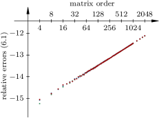
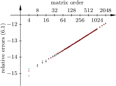
Figure 2: The relative errors (25), in $\log_{10}$-scale, in the HSVD computed in DOUBLE PRECISION (left) and DOUBLE COMPLEX (right) datatypes. The matrix orders on $x$-axis are in $\log_{2}$-scale.

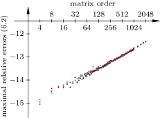
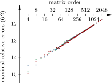
Figure 3: The maximal relative errors (26), in $\log_{10}$-scale, in the eigenvalues of $G_{0}J_{0}G_{0}^{\ast}$, with the $J_{0}$-HSVD of $G_{0}$ computed in DOUBLE PRECISION (left) and DOUBLE COMPLEX (right) datatypes. The matrix orders on $x$-axis are in $\log_{2}$-scale.

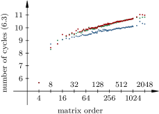
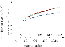
Figure 4: The number of cycles (27) until convergence, when computing in DOUBLE PRECISION (left) and DOUBLE COMPLEX (right) datatypes. The matrix orders on $x$-axis are in $\log_{2}$-scale.

A comparison of the relative errors in the decomposition, shown in Figure 2, leads to a similar conclusion that can be reached by comparing the maximal relative errors in the eigenvalues of $H$, shown in Figure 3. In the real as well as in the complex case a satisfactory accuracy, in a sense of both (25) and (26), was reached in a reasonably small number of cycles, as shown in Figure 4.

A sequential (with $t=1$) variant of the algorithm, performing one step at a time, was compared performance-wise against the parallel multi-step one, with $\upsilon=0.75$ and $n_{0}$ going up to $128$ and $256$ for $T=\mathbb{C}$ and $T=\mathbb{R}$, respectively. The sequential variant was drastically slowed down (up to more than three orders of magnitude) compared to the multi-step one, especially for the “true” HSVD (less so for the “ordinary” SVD), to a point of being totally impractical. The $J$-Kogbetliantz algorithm is therefore best run in the multi-step regime, with as much parallelism as possible.

7 Conclusions and future work

In this paper an accurate method for computing the $2\times 2$ HSVD of real and complex matrices is demonstrated and employed as one of the three major building blocks of a $J$-Kogbetliantz algorithm for general square matrices. The other two important contributions are a heuristic but efficient convergence criterion for all pointwise Kogbetliantz-type processes and a modification of the well-established dynamic pivot strategy that can cope with the pivot weights of arbitrary magnitudes and signs.

To keep the exposition concise, a forward rounding error analysis of the floating-point computation of the $2\times 2$ HSVD is left for future work. Furthermore, performing such analysis is slightly impeded by, e.g., a lack of standardized, tight error bounds for the absolute value of a complex number, or equivalently, of the $\mathtt{HYPOT}$ intrinsic.

The $J$-Kogbetliantz algorithm, as presented, is not highly performant even in its parallel form. It is worth exploring if (and what kind of) blocking of the algorithm would be beneficial in terms of performance, without negatively affecting accuracy. A straightforward generalization of the dynamic pivot strategy to block (instead of $2\times 2$) pivots seems too inefficient, as it would assume at each block-multi-step the full diagonalization of all possible block pivots that require hyperbolic transformations only to compute their weights. Apart from—and complementary to—blocking, there are other options for improving performance, like storing and reusing the $2\times 2$ HSVDs computed while forming a multi-step, as explained in section 3, and implementing a vectorized sorting routine for the suitably represented augmented weights.

The batches of $2\times 2$ transformations in each multi-step could be processed in a vectorized way, as in Novakovic-20 , should a highly optimized implementation be required. Such a version of the algorithm would have to resort to a specific vectorized routine in each of the three cases of $2\times 2$ transformations (one trigonometric and two hyperbolic, of lower and upper triangular matrices). Consequently, (up to) three disjoint batches would have to be processed separately, with a non-trivial repacking of input data for each of them. A serious practical use-case is required to justify such effort.

Finally, an interesting observation is offered without a proof. For complex matrices, the $J$-Kogbetliantz algorithm seems to converge (in limit) not only in the sense of $\mathop{\mathrm{off}_{F}^{2}}(G_{k})\to 0$ and $\mathop{\mathrm{diag}}(G_{k})\to\Sigma$, but also with $\displaystyle\max_{i\neq j}|\arg(G_{k})_{ij}|\to 0$, for $k\to\infty$.

Declarations

Appendix A Proofs of Lemmas 1 and 2

Proof (Lemma 1)

Let, for $1\leq\ell\leq n$, $\gamma_{\ell}=\arg(x_{\ell})$ and $\delta_{\ell}=\arg(y_{\ell})$. Then,

$$\begin{bmatrix}x_{\ell}&y_{\ell}\end{bmatrix}=\begin{bmatrix}e^{\mathrm{i}\gamma_{\ell}}|x_{\ell}|&e^{\mathrm{i}\delta_{\ell}}|y_{\ell}|\end{bmatrix}=e^{\mathrm{i}\gamma_{\ell}}\begin{bmatrix}|x_{\ell}|&e^{\mathrm{i}(\delta_{\ell}-\gamma_{\ell})}|y_{\ell}|\end{bmatrix}=e^{\mathrm{i}\delta_{\ell}}\begin{bmatrix}e^{\mathrm{i}(\gamma_{\ell}-\delta_{\ell})}|x_{\ell}|&|y_{\ell}|\end{bmatrix}.$$

Using the second equality, from the matrix multiplication it follows

$$x_{\ell}^{\prime}=e^{\mathrm{i}\gamma_{\ell}}(|x_{\ell}|\cosh\psi+e^{\mathrm{i}(\delta_{\ell}-\gamma_{\ell}-\beta)}|y_{\ell}|\sinh\psi),$$

and using the third equality, from the matrix multiplication it follows

$$y_{\ell}^{\prime}=e^{\mathrm{i}\delta_{\ell}}(e^{\mathrm{i}(\gamma_{\ell}-\delta_{\ell}+\beta)}|x_{\ell}|\sinh\psi+|y_{\ell}|\cosh\psi).$$

Since $|e^{-\mathrm{i}\gamma_{\ell}}x_{\ell}^{\prime}|=|x_{\ell}^{\prime}|$ and $|e^{-\mathrm{i}\delta_{\ell}}y_{\ell}^{\prime}|=|y_{\ell}^{\prime}|$ and $\cos(-\phi)=\cos\phi$, it holds

$$|x_{\ell}^{\prime}|^{2} =(|x_{\ell}|\cosh\psi+\cos(\delta_{\ell}-\gamma_{\ell}-\beta)|y_{\ell}|\sinh\psi)^{2}+(\sin(\delta_{\ell}-\gamma_{\ell}-\beta)|y_{\ell}|\sinh\psi)^{2}$$

$$=|x_{\ell}|^{2}\cosh^{2}\psi+|y_{\ell}|^{2}\sinh^{2}\psi+\cos(\delta_{\ell}-\gamma_{\ell}-\beta)|x_{\ell}||y_{\ell}|2\cosh\psi\sinh\psi,$$

$$|y_{\ell}^{\prime}|^{2} =(\cos(\gamma_{\ell}-\delta_{\ell}+\beta)|x_{\ell}|\sinh\psi+|y_{\ell}|\cosh\psi)^{2}+(\sin(\gamma_{\ell}-\delta_{\ell}+\beta)|x_{\ell}|\sinh\psi)^{2}$$

$$=|x_{\ell}|^{2}\sinh^{2}\psi+|y_{\ell}|^{2}\cosh^{2}\psi+\cos(\delta_{\ell}-\gamma_{\ell}-\beta)|x_{\ell}||y_{\ell}|2\cosh\psi\sinh\psi.$$

After grouping the terms, the square of the Frobenius norm of the new $\ell$th row is

$$\left\|\begin{bmatrix}x_{\ell}^{\prime}&y_{\ell}^{\prime}\end{bmatrix}\right\|_{F}^{2}=|x_{\ell}^{\prime}|^{2}+|y_{\ell}^{\prime}|^{2} =(\cosh^{2}\psi+\sinh^{2}\psi)(|x_{\ell}|^{2}+|y_{\ell}|^{2})$$ (28)

$$+2\cos(\delta_{\ell}-\gamma_{\ell}-\beta)|x_{\ell}||y_{\ell}|2\cosh\psi\sinh\psi.$$

Summing the left side of the equation (28) over all $\ell$ one obtains

$$\left\|\begin{bmatrix}\mathbf{x}^{\prime}&\mathbf{y}^{\prime}\end{bmatrix}\right\|_{F}^{2}=\sum_{\ell=1}^{n}\left(|x_{\ell}^{\prime}|^{2}+|y_{\ell}^{\prime}|^{2}\right),$$

what is equal to the right side of the equation (28), summed over all $\ell$,

$$\sum_{\ell=1}^{n}\left((\cosh^{2}\psi+\sinh^{2}\psi)(|x_{\ell}|^{2}+|y_{\ell}|^{2})+2\zeta_{\ell}|x_{\ell}||y_{\ell}|2\cosh\psi\sinh\psi\right),$$

where $-1\leq\zeta_{\ell}=\cos(\delta_{\ell}-\gamma_{\ell}-\beta)\leq 1$, so $|\zeta_{\ell}|\leq 1$. The last sum can be split into a non-negative part and the remaining part of an arbitrary sign,

$$(\cosh^{2}\psi+\sinh^{2}\psi)\sum_{\ell=1}^{n}(|x_{\ell}|^{2}+|y_{\ell}|^{2})+2\cosh\psi\sinh\psi\sum_{\ell=1}^{n}2\zeta_{\ell}|x_{\ell}||y_{\ell}|.$$

Using the triangle inequality, and observing that $\sum_{\ell=1}^{n}(|x_{\ell}|^{2}+|y_{\ell}|^{2})=\left\|\begin{bmatrix}\mathbf{x}&\mathbf{y}\end{bmatrix}\right\|_{F}^{2}$, this value can be bounded above by

$$(\cosh^{2}\psi+\sinh^{2}\psi)\left\|\begin{bmatrix}\mathbf{x}&\mathbf{y}\end{bmatrix}\right\|_{F}^{2}+2\cosh\psi|\sinh\psi|\sum_{\ell=1}^{n}2|x_{\ell}||y_{\ell}|,$$

and below by

$$(\cosh^{2}\psi+\sinh^{2}\psi)\left\|\begin{bmatrix}\mathbf{x}&\mathbf{y}\end{bmatrix}\right\|_{F}^{2}-2\cosh\psi|\sinh\psi|\sum_{\ell=1}^{n}2|x_{\ell}||y_{\ell}|,$$

where both bounds can be simplified by the identities

$$\cosh^{2}\psi+\sinh^{2}\psi=\cosh(2\psi),\qquad 2\cosh\psi|\sinh\psi|=|\sinh(2\psi)|.$$

By the inequality of arithmetic and geometric means it holds $2|x_{\ell}||y_{\ell}|\leq(|x_{\ell}|^{2}+|y_{\ell}|^{2})$, so a further upper bound is reached as

$$\cosh(2\psi)\left\|\begin{bmatrix}\mathbf{x}&\mathbf{y}\end{bmatrix}\right\|_{F}^{2}+|\sinh(2\psi)|\left\|\begin{bmatrix}\mathbf{x}&\mathbf{y}\end{bmatrix}\right\|_{F}^{2},$$

and a further lower bound as

$$\cosh(2\psi)\left\|\begin{bmatrix}\mathbf{x}&\mathbf{y}\end{bmatrix}\right\|_{F}^{2}-|\sinh(2\psi)|\left\|\begin{bmatrix}\mathbf{x}&\mathbf{y}\end{bmatrix}\right\|_{F}^{2},$$

what, after grouping the terms and dividing by $\left\|\begin{bmatrix}\mathbf{x}&\mathbf{y}\end{bmatrix}\right\|_{F}^{2}$, concludes the proof. ∎

Proof (Lemma 2)

Note that $\cosh(2\psi)+|\sinh(2\psi)|\geq\cosh(2\psi)\geq 1$, and

$$1 =\cosh^{2}(2\psi)-\sinh^{2}(2\psi)$$

$$=(\cosh(2\psi)-|\sinh(2\psi)|)\cdot(\cosh(2\psi)+|\sinh(2\psi)|)$$

$$\geq\cosh(2\psi)-|\sinh(2\psi)|>0.$$

If $\psi=0$, the equalities in the bounds established in Lemma 1 hold trivially. Also, if both equalities hold simultaneously, $\psi=0$.

The inequality of arithmetic and geometric means in the proof of Lemma 1 turns into equality if and only if $|x_{\ell}|=|y_{\ell}|$ for all $\ell$. When $|x_{\ell}||y_{\ell}|\neq 0$, it has to hold $\zeta_{\ell}=\zeta$, where $\zeta=\pm\mathop{\mathrm{sign}}(\sinh\psi)$, to reach the upper or the lower bound, respectively. From $\zeta=\pm 1$ it follows $\delta_{\ell}=\gamma_{\ell}+\beta+l\pi$ for a fixed $l\in\mathbb{Z}$, i.e., $x_{\ell}=e^{\mathrm{i}\gamma_{\ell}}|x_{\ell}|$ and $y_{\ell}=\pm e^{\mathrm{i}\beta}e^{\mathrm{i}\gamma_{\ell}}|x_{\ell}|$, so $y_{\ell}=\pm e^{\mathrm{i}\beta}x_{\ell}$ for all $\ell$. Conversely, $\mathbf{y}=\pm e^{\mathrm{i}\beta}\mathbf{x}$ implies, for all $\ell$, that $|x_{\ell}|=|y_{\ell}|$ and $\zeta_{\ell}$ is a constant $\zeta=\pm 1$, so one of the two bounds is reached. ∎

References

• (1) Anderson, E., Bai, Z., Bischof, C., Blackford, S., Demmel, J., Dongarra, J., Du Croz, J., Greenbaum, A., Hammarling, S., McKenney, A., Sorensen, D.: LAPACK Users’ Guide, $3^{\rm rd}$ edn. Software, Environments and Tools. Society for Industrial and Applied Mathematics, Philadelphia, PA, USA (1999). DOI 10.1137/1.9780898719604
• (2) Baudet, G., Stevenson, D.: Optimal sorting algorithms for parallel computers. IEEE Trans. Comput. C-27(1), 84–87 (1978). DOI 10.1109/TC.1978.1674957
• (3) Bečka, M., Okša, G., Vajteršic, M.: Dynamic ordering for a parallel block-Jacobi SVD algorithm. Parallel Comp. 28(2), 243–262 (2002). DOI 10.1016/S0167-8191(01)00138-7
• (4) Bojanczyk, A.W., Onn, R., Steinhardt, A.O.: Existence of the hyperbolic singular value decomposition. Linear Algebra Appl. 185(C), 21–30 (1993). DOI 10.1016/0024-3795(93)90202-Y
• (5) Charlier, J.P., Vanbegin, M., Van Dooren, P.: On efficient implementations of Kogbetliantz’s algorithm for computing the singular value decomposition. Numer. Math. 52(3), 279–300 (1987). DOI 10.1007/BF01398880
• (6) Drmač, Z.: Implementation of Jacobi rotations for accurate singular value computation in floating point arithmetic. SIAM J. Sci. Comput. 18(4), 1200–1222 (1997). DOI 10.1137/S1064827594265095
• (7) Hari, V., Matejaš, J.: Accuracy of two SVD algorithms for $2\times 2$ triangular matrices. Appl. Math. Comput. 210(1), 232–257 (2009). DOI 10.1016/j.amc.2008.12.086
• (8) Hari, V., Singer, S., Singer, S.: Block-oriented $J$-Jacobi methods for Hermitian matrices. Linear Algebra Appl. 433(8–10), 1491–1512 (2010). DOI 10.1016/j.laa.2010.06.032
• (9) Hari, V., Singer, S., Singer, S.: Full block $J$-Jacobi method for Hermitian matrices. Linear Algebra Appl. 444, 1–27 (2014). DOI 10.1016/j.laa.2013.11.028
• (10) Hari, V., Veselić, K.: On Jacobi methods for singular value decompositions. SIAM J. Sci. Stat. 8(5), 741–754 (1987). DOI 10.1137/0908064
• (11) Hari, V., Zadelj-Martić, V.: Parallelizing the Kogbetliantz method: A first attempt. J. Numer. Anal. Ind. Appl. Math. 2(1–2), 49–66 (2007)
• (12) IEEE Computer Society: 754-2019 - IEEE Standard for Floating-Point Arithmetic. IEEE, 3 Park Avenue, New York, NY 10016-5997, USA (2019). DOI 10.1109/IEEESTD.2019.8766229
• (13) ISO/IEC JTC1/SC22/WG5: ISO/IEC 1539-1:2018(en) Information technology — Programming languages — Fortran — Part 1: Base language, $4^{\rm th}$ edn. ISO (2018). International standard.
• (14) Kogbetliantz, E.G.: Solution of linear equations by diagonalization of coefficients matrix. Quart. Appl. Math. 13(2), 123–132 (1955). DOI 10.1090/qam/88795
• (15) Kulikov, G.Yu., Kulikova, M.V.: Hyperbolic-singular-value-decomposition-based square-root accurate continuous-discrete extended-unscented Kalman filters for estimating continuous-time stochastic models with discrete measurements. Int. J. Robust Nonlinear Control 30, 2033–2058 (2020). DOI 10.1002/rnc.4862
• (16) Kulikova, M.V.: Hyperbolic SVD-based Kalman filtering for Chandrasekhar recursion. IET Control Theory A. 13(10), 1525–1531 (2019). DOI 10.1049/iet-cta.2018.5864
• (17) Kulikova, M.V.: Square-root approach for Chandrasekhar-based maximum correntropy Kalman filtering. IEEE Signal Process Lett. 26(12), 1803–1807 (2019). DOI 10.1109/LSP.2019.2948257
• (18) Mackey, D.S., Mackey, N., Tisseur, F.: Structured factorizations in scalar product spaces. SIAM J. Matrix Anal. and Appl. 27(3), 821–850 (2005). DOI 10.1137/040619363
• (19) Matejaš, J., Hari, V.: Accuracy of the Kogbetliantz method for scaled diagonally dominant triangular matrices. Appl. Math. Comput. 217(8), 3726–3746 (2010). DOI 10.1016/j.amc.2010.09.020
• (20) Matejaš, J., Hari, V.: On high relative accuracy of the Kogbetliantz method. Linear Algebra Appl. 464, 100–129 (2015). DOI 10.1016/j.laa.2014.02.024
• (21) Novaković, V.: A hierarchically blocked Jacobi SVD algorithm for single and multiple graphics processing units. SIAM J. Sci. Comput. 37(1), C1–C30 (2015). DOI 10.1137/140952429
• (22) Novaković, V.: Batched computation of the singular value decompositions of order two by the AVX-512 vectorization. Parallel Process. Lett. 30(4), 2050015 (2020). DOI 10.1142/S0129626420500152
• (23) Novaković, V., Singer, S.: A GPU-based hyperbolic SVD algorithm. BIT 51(4), 1009–1030 (2011). DOI 10.1007/s10543-011-0333-5
• (24) NVIDIA Corp.: CUDA C++ Programming Guide v10.2.89 (November 2019). URL https://docs.nvidia.com/cuda/cuda-c-programming-guide/
• (25) Okša, G., Yamamoto, Y., Bečka, M., Vajteršic, M.: Asymptotic quadratic convergence of the two-sided serial and parallel block-Jacobi SVD algorithm. SIAM J. Matrix Anal. and Appl. 40(2), 639–671 (2019). DOI 10.1137/18M1222727
• (26) Onn, R., Steinhardt, A.O., Bojanczyk, A.W.: The hyperbolic singular value decomposition and applications. IEEE Trans. Signal Process. 39(7), 1575–1588 (1991). DOI 10.1109/78.134396
• (27) OpenMP ARB: OpenMP Application Programming Interface Version 5.0 (November 2018). URL https://www.openmp.org/wp-content/uploads/OpenMP-API-Specification-5.0.pdf
• (28) Singer, S.: Indefinite QR factorization. BIT 46(1), 141–161 (2006). DOI 10.1007/s10543-006-0044-5
• (29) Singer, S., Di Napoli, E., Novaković, V., Čaklović, G.: The LAPW method with eigendecomposition based on the Hari–Zimmermann generalized hyperbolic SVD. SIAM J. Sci. Comput. 42(5), C265–C293 (2020). DOI 10.1137/19M1277813
• (30) Singer, S., Singer, S., Novaković, V., Davidović, D., Bokulić, K., Ušćumlić, A.: Three-level parallel $J$-Jacobi algorithms for Hermitian matrices. Appl. Math. Comput. 218(9), 5704–5725 (2012). DOI 10.1016/j.amc.2011.11.067
• (31) Singer, S., Singer, S., Novaković, V., Ušćumlić, A., Dunjko, V.: Novel modifications of parallel Jacobi algorithms. Numer. Algorithms 59(1), 1–27 (2012). DOI 10.1007/s11075-011-9473-6
• (32) Slapničar, I.: Accurate symmetric eigenreduction by a Jacobi method. Ph.D. thesis, FernUniversität–Gesamthochschule, Hagen (1992)
• (33) Slapničar, I.: Componentwise analysis of direct factorization of real symmetric and Hermitian matrices. Linear Algebra Appl. 272, 227–275 (1998). DOI 10.1016/S0024-3795(97)00334-0
• (34) Stewart, G.W.: An updating algorithm for subspace tracking. IEEE Trans. Signal Process. 40(6), 1535–1541 (1992). DOI 10.1109/78.139256
• (35) Veselić, K.: A Jacobi eigenreduction algorithm for definite matrix pairs. Numer. Math. 64(1), 241–269 (1993). DOI 10.1007/BF01388689
• (36) Zha, H.: A note on the existence of the hyperbolic singular value decomposition. Linear Algebra Appl. 240, 199–205 (1996). DOI 10.1016/0024-3795(94)00197-9