Cohesive Networks using Delayed Self Reinforcement

Abstract

How a network gets to the goal (a consensus value) can be as important as reaching the consensus value. While prior methods focus on rapidly getting to a new consensus value, maintaining cohesion, during the transition between consensus values or during tracking, remains challenging and has not been addressed. The main contributions of this work are to address the problem of maintaining cohesion by: (i) proposing a new delayed self-reinforcement (DSR) approach; (ii) extending it for use with agents that have higher-order, heterogeneous dynamics, and (iii) developing stability conditions for the DSR-based method. With DSR, each agent uses current and past information from neighbors to infer the overall goal, and modifies the update law to improve cohesion. The advantages of the proposed DSR approach are that it only requires already-available information from a given network to improve the cohesion, and does not require network-connectivity modifications (which might not be always feasible) nor increases in the system’s overall response speed (which can require larger input). Moreover, illustrative simulation examples are used to comparatively evaluate the performance with and without DSR. The simulation results show substantial improvement in cohesion with DSR.

1 Introduction

The goal of this work is to enable cohesive transitions in multi-agent networks, e.g., to enable similar response in each agent when transitioning from one consensus value to another. How a network gets to the final goal (i.e., cohesion during the transition) can be as important as reaching the final goal, e.g., to maintain specified inter-vehicle spacing in connected, automated transportation systems [1, 2], to align the orientation of agents during maneuvers of flocks and swarms in nature, e.g., [3, 4, 5], and to maintain formation of engineered networks such as satellites, unmanned autonomous vehicles and collaborative robots [6, 7, 8, 9, 10, 11]. While prior methods aim to achieve rapid convergence to a consensus goal, cohesion during transitions between the consensus values has not been addressed and remains challenging. The loss of cohesion during transitions arises because information about the desired change (such as the desired orientation or speed) in the goal might be available to only a few agents in the network and needs to diffuse through the system. The resulting response-time delays, between agents that are “close”  to the information source in the network and those that are “farther away”, lead to loss of cohesion during the transition, even though they all reach the final goal. The impact of transition-cohesion loss can be mitigated by using additional control effort, e.g., designed to maintain inter-agent spacing and reduce formation distortions [6, 7, 8]. Nevertheless, a cohesive transient response, when feasible, reduces the need for such additional control effort. Moreover, in biological systems, the alignment response is transmitted faster than neighbor-to-neighbor re-arrangements [5], which indicates that cohesion improvements (e.g., in the alignment response) during the transitions might be more effective than the slower rearrangements of the agents (or other actions) to correct for the loss of cohesion during rapid maneuvers. This potential reduction in overall effort by maintaining cohesion motivates the current study aimed at improving transition cohesion.

Faster convergence to the new consensus value can improve transition cohesion. For example, faster convergence implies a smaller overall settling time of the network response during transitions between consensus values. Here, the settling time is the time needed for all agents to reach within a specified percentage of a final consensus state $Z=Z_{f}$ when transitioning from an initial consensus state $Z=Z_{i}$, where all agents have the same initial value. Faster settling reduces the potential delays between the responses of the agents, and in this sense, promotes cohesion. For example, the network’s response can be speeded up when the network dynamics has the form,

$$\dot{Z}(t)=U(t)=-\gamma\hat{K}Z(t)+\gamma\hat{B}z_{s}(t)$$ (1)

by scaling up the gain $\gamma$ of the network interactions, where $K=\gamma\hat{K}$ is the graph Laplacian and $z_{s}$ is the desired response. Nonlinear methods have also been proposed to achieve linear and finite time convergence, e.g., [12, 13, 14, 15]. However, in general, increasing the overall speed of the network requires larger inputs $U$. Therefore, maximum-input constraints on the actuators can lead to restrictions on the maximum response-speed increase, which in turn limits the achievable cohesion.

The response speed, and therefore, transition cohesion can be improved if there is choice in the structure of the network. For example, if spatially-distant agents can be connected, then the information about changes in the desired response $z_{s}$ can spread faster, which can improve cohesion of agent responses. Similarly, a faster response can be achieved by optimally selecting the Laplacian $K$, e.g., as in [16]. Time-varying connections such as randomized interconnections also can lead to a faster response, e.g., [17]. Moreover, connectivity enhancements have been proposed for jointly-connected networks  [18]. Nevertheless, when such time-variations in the graph structure or selection of the graph Laplacian $K$ are not feasible (e.g., when a given structure has to be used), the range of acceptable update gain $\gamma$, e.g., due to input bounds, can limit the response speed. Finally, although speeding up the response leads to smaller loss of cohesion, the response-time delays are still present in the faster response. Cohesion, normalized by the settling time, does not necessarily improve. The lack of cohesion, even with faster response and potential limits due to actuator constraints, motivates the current effort to improve cohesion without the typical emphasis on increasing the response speed.

Ideally, for cohesion, all agents should be directly connected to the source. Then, every agent has immediate access to the desired response, i.e., $z_{s}$. However, this requires broadcasting the source information across spatially distant neighbors that might not be feasible in large networks. Moreover, such broadcasting might not be preferred in the presence of adversaries since they could then infer the intent of the network. The cohesion problem addressed here is to achieve a uniform response across the network (to changes in the source), and each agent uses information from its neighbors without requiring additional knowledge about the overall network connections.

Previous work has shown that cohesion can be improved by using derivative information from the neighbors of each agent, see [1]. In such a setting, the control input for an agent $i$, contains derivative information from its neighbors $N_{i}$, which in turn depend on derivative information from other neighbors $k\notin N_{i}$. Therefore, each agent $i$ cannot independently compute its update $\dot{z}_{i}$ by only knowing information about its immediate neighbors $N_{i}$. It is shown in this article that the proposed, delayed self reinforcement (DSR), effectively approximates the derivative information from the neighbors needed for response cohesion. Such use of delayed information has been used in artificial neural networks for improving gradient-based learning algorithms [19, 20]. Similar use of delayed information can improve network response speeds under update-bandwidth limitations for discrete-time multi-agent systems, e.g., as shown in  [21]. The novelty in the current work is the use of DSR to improve cohesion using already-available information from a given network, without requiring network-connectivity modifications or increases in the response speed.

The main contribution of this work is the development of stability conditions for the proposed delayed self-reinforcement (DSR) approach. The delay in the implementation turns the dynamics of the networked system into a delay-differential-equation (DDE). Note that DDEs have been well studied in the past, e.g.,  [22, 23], and numerical methods are available using the Lambert W function [24] to evaluate the stability of DDEs, e.g. see [25, 26]. For example, derivative control, used to improve robustness of single-input-single-output systems, can be implemented using delay-based approximation as in [27], and stability can be inferred using the Lambert W function. Approaches have also been developed to find the range of time-delays under which stability is maintained for a DDE, e.g., [28, 29, 30, 31]. Nevertheless, it is challenging to develop general stability conditions for DDEs. For special cases, e.g., when the matrices involved in the DDEs are symmetric (which corresponds to the underlying graph associated with the Laplacian $K$ being undirected in the current application) stability conditions can be developed, e.g., as in [32]. The current paper develops generalized stability conditions for the DDE associated with the DSR approach for, both, directed and undirected graphs. These stability conditions are developed by exploiting the graph structure of the network and the results depend on the eigenvalues of the associated graph Laplacian $K$. In this sense it extends Brayton’s stability results for DDEs  [32] to the more general case with non-symmetric matrices, which can be applied to directed graphs. Moreover, the article shows that when the eigenvalues of the Laplacian $K$ are real, e.g., for undirected graphs or directed but topologically ordered sub-graphs (defined later in this article), (i)  the stability conditions developed in this article for the network with DSR reduce to the results for scalar DDEs from [33], and (ii) the proposed DSR approach is stable independent of the delay. Lastly, the proposed DSR approach is applicable to cases when the agent dynamics is heterogenous and higher order, but with the same relative degree.

2 Cohesive-response problem

The network dynamics is defined using a graph representation in this section. Then, the cohesion in the response dynamics is quantified and the problem of improving the cohesion is posed.

2.1 Graph-based response dynamics

Let the connectivity of the agents be represented by a directed graph (digraph) ${\mathcal{G}}=\left({\mathcal{V}},{\mathcal{E}}\right)$, e.g., as defined in [34], with agents represented by nodes ${\mathcal{V}}=\left\{1,2,\ldots,{n\!+\!1}\right\}$, $n>1$ and edges ${\mathcal{E}}\subseteq{\mathcal{V}}\times{\mathcal{V}}$, where the neighbors of the agent $i$ are represented by the set $N_{i}=\{k\in{\mathcal{V}},k\neq i:(k,i)\in{\mathcal{E}}\}$. Node $s$, which is assumed, without loss of generality, to be the last node, represents the desired response, $z_{s}$. The terms $l_{ik}$ of the $(n+1)\times(n+1)$ Laplacian $L$ of the graph ${\mathcal{G}}$ are real and given by

$$l_{ik} =\left\{\begin{array}[]{ll}-w_{ik},&{\mbox{if}}~{}k\in N_{i}\\ \sum_{m=1}^{n+1}w_{im},&{\mbox{if}}~{}k=i,\\ 0&{\mbox{otherwise, }}\end{array}\right.$$ (5)

where the weights $w_{ik}$ are positive if $k\in N_{i}$ and zero otherwise. The dynamics for the non-source agents $Z$ (with each agent state-component given by $z_{i}$), represented by the graph ${\mathcal{G}}\!\setminus\!s$, can be written in matrix form as

$$\frac{d{Z}}{dt}(t)=\dot{Z}(t) =U=-KZ(t)+Bz_{s}(t),$$ (6)

similar to Eq. (1), where $U$ is the input to the agents. The $n\times n$ matrix $K$ (the pinned Laplacian) is obtained by removing the row and column associated with the source node $n+1$ through the following partitioning of the graph Laplacian $L$, i.e.,

$$L =\left[\begin{array}[]{c|c}K&-B\\ \hline\cr\star_{1\times n}&\star_{1\times 1}\end{array}\right]$$ (9)

with $B$ an $n\times 1$ input matrix, $B=[w_{1,s},w_{2,s},\ldots,w_{n,s}]^{T}~{}=[B_{1},B_{2},\ldots,B_{n}]^{T}$.

2.2 Graph properties

Some standard graph properties (needed later), resulting from the following assumption, are described below.

Assumption 1 (Connected to source node).

The digraph ${\mathcal{G}}$ is assumed to have a directed path from the source node $s$ to any node $i\in{\mathcal{V}}\setminus\!s$.

From Assumption 1 and the Matrix-Tree Theorem in [35] the pinned Laplacian $K$ of the graph without the source node $s$ is invertible, i.e., $\det{(K)}\neq 0$. The eigenvalues $\left\{\lambda_{K,i}\right\}_{i=1}^{n}$ of pinned Laplacian $K$ have strictly-positive, real parts, i.e.,

$${{\mathcal{R}}e}\left({\lambda_{K,i}}\right) >0,$$ (10)

and therefore the negative of the pinned Laplacian (i.e., $-K$) is Hurwitz, with eigenvalues on the open left half of the complex plane. This follows from the Gershgorin theorem since all the eigenvalues of the pinned Laplacian $K$ must lie in one of circles centered at $l_{ii}>0$ with radius $l_{ii}-w_{is}\in[0,l_{ii}]$ from definition of $l_{ii}$ in Eq. (5) and $w_{is}\geq 0$. Given the invertibility of pinned Laplacian $K$, the eigenvalues of the pinned Laplacian $K$ cannot be at the origin, and therefore the eigenvalues must have strictly positive real parts (from the Gershgorin theorem condition of being inside the circles which are on the right hand side of the complex place except for the origin).

The product of the inverse of the pinned Laplacian $K$ with $B$ leads to a $n\times 1$ vector of ones, i.e., $K^{-1}B={\textbf{1}}_{n}$, which follows from the partitioning in Eq. (9), and invertibility of $K$ since the $(n+1)\times 1$ vector of ones ${\textbf{1}}_{n+1}=[1,\ldots,1]^{T}$ is a right eigenvector of the Laplacian $L$ with eigenvalue $0$, i.e., $L{\textbf{1}}_{n+1}=0{\textbf{1}}_{n+1},$ resulting in

$$K{\textbf{1}}_{n} =B.$$ (11)

2.3 Quantifying cohesion

Lack of cohesion is quantified in terms of the deviations $\Delta$ in the responses between agents for a step change in the source $z_{s}$ from $z_{s}(0)=0$ at time $t=0$ to $z_{s}(t)=z_{d}\neq 0$ for time $t>0$. The response of the non-source agents, i.e., solution to Eq. (6), can be written as

$$Z(t) =e^{-Kt}Z(0)+(-K)^{-1}\left[e^{-Kt}-I\right]Bz_{d},$$ (12)

which simplifies to

$$Z(t) =(-K)^{-1}\left[e^{-Kt}-I\right]Bz_{d}$$ (13)

if the initial state $Z(0)$ is at consensus, i.e., $Z(0)=0$. Note that the exponent $e^{-Kt}\rightarrow 0$ as time increases since the negative of the pinned Laplacian $-K$ is Hurwitz. Therefore, from Eq. (11), the response $Z(t)$, of the non-source agents, exponentially reaches the desired value $z_{d}$ as time $t$ increases, i.e,

$$Z(t) \rightarrow z_{d}{\textbf{1}}_{n}~{}~{}{\mbox{as}}~{}~{}t\rightarrow\infty.$$ (14)

The lack of cohesion can be quantified in terms of the deviations $\Delta$ in the response as

$$\Delta =\frac{1}{z_{d}}\int_{0}^{T_{s}}\left|Z(t)-\overline{z}(t){\textbf{1}}_{n}\right|_{1}dt,$$ (15)

where $T_{s}$ is the settling time, i.e., the time by which all agent responses $Z$ reach and stay within $2\%$ of the final value $z_{d}$, $\overline{z}$ is the average value of the state $Z$, over all individual agent state-components $z_{i}$, i.e.,

$$\overline{z}(t) =\frac{1}{n}\sum_{i=1}^{n}z_{i}(t),$$ (16)

and $|\cdot|_{1}$ is the standard vector 1-norm, $|\hat{Z}|_{1}=\sum_{i=1}^{n}|\hat{z}_{i}|$ for any vector $\hat{Z}$. A normalized measure ${\Delta}^{*}$ that removes the effect of the response speed is obtained by dividing the expression in Eq. (15) with the settling time $T_{s}$ as

$${\Delta}^{*} =\frac{\Delta}{T_{s}}.$$ (17)

Note that the system’s transient response is more cohesive if the normalized deviation ${\Delta}^{*}$ is small.

2.4 Problem: reduce normalized deviation ${\Delta}^{*}$

The research problem is to improve cohesion (i.e., to reduce the normalized deviation ${\Delta}^{*}$) without changing the network connectivity or access to the information source, i.e., without changing the network graph ${\mathcal{G}}$.

3 Proposed approach

3.1 Ideal cohesive dynamics

If each non-source agent can have instantaneous access to the source $z_{s}$

$$\dot{z}_{i}(t) =-\alpha{z}_{i}(t)+\alpha z_{s}(t),$$ (18)

then with the same initial condition, the response of all the agents would be cohesive. In particular, the entire system will respond to a step input, $z_{s}(0)=0$ at time $t=0$ to $z_{s}(t)=z_{d}\neq 0$ for time $t>0$ with a zero initial state $z_{i}(0)=0$, in a cohesive manner. Moreover, each agent state $z_{i}$ will have the same settling time (to reach and stay within 2% of the final value)

$$T_{s}=\frac{4}{\alpha},$$ (19)

provided, for stability, $\alpha>0$. Note that the parameter $\alpha$ can be used to adjust the overall speed of the response of each agent. In a vector form, this ideal cohesive dynamics can be written as

$$\dot{Z}(t) =-\alpha Z(t)+\alpha{\textbf{1}}_{n}z_{s}(t).$$ (20)

Multiplying both sides of Eq. (20) by $\beta K$ (where $\beta>0$) and using Eq. (11) to replace $K{\textbf{1}}_{n}$ results in

$$\beta K\dot{Z}(t) =-\alpha\beta KZ(t)+\alpha\beta K{\textbf{1}}_{n}z_{s}(t)~{}~{}=-\alpha\beta KZ(t)+\alpha\beta Bz_{s}(t),$$ (21)

and therefore, by adding $\dot{Z}$ on both sides, the ideal cohesive dynamics can be rewritten as

$$\dot{Z}(t) =-\alpha\beta KZ(t)+\alpha\beta Bz_{s}(t)+\left[I-\beta K\right]\dot{Z}(t).$$ (22)

Remark 1 (Network connectivity and improved cohesion).

The ideal cohesive dynamics in Eq. (22) is found by exploiting the network connectivity (i.e., invertibility of the pinned Laplacian, and convergence to consensus), which enables the replacement of $K{\textbf{1}}_{n}$ by $B$ in Eq. (21). As a result, all agents have the same time-trajectory solution as in Eq. (20) (provided the system is initially synchronized) even with rapid changes in the source $z_{s}$. Therefore, the normalized deviation in (17) is zero with the ideally cohesive dynamics in Eq. (22), i.e.,

$${\Delta}^{*}=0.$$

In this sense, the DSR approach (presented below) accounts for network issues such as potential redundancy of information obtained from neighbors. ∎

The measure of cohesion ${\Delta}^{*}$ does not capture the convergence rate to the final value, which depends on (and can be adjusted by the selection of) the parameter $\alpha$ in Eq. (20).

3.2 Delay-based derivative

The idealized control law in Eq. (22) is implemented in the following with delayed self reinforcement (DSR). The input for an agent $i$, from the right hand side of the expression in Eq. (22), contains derivative information from its neighbors $N_{i}$, which in turn depends on other agents $k$ that might not be a neighbor of agent $i$, i.e., $k\notin N_{i}$. Therefore, it is challenging to compute, and implement the ideal cohesive dynamics in Eq. (22). A delay-based implementation of the derivative is discussed below.

Consider the approximate implementation of the derivative $\dot{Z}(t)$ in right-hand-side of Eq. (22) by using a delay, $\tau>0,$ as

$$\dot{Z}(t) \approx\frac{Z(t)-Z(t-\tau)}{\tau}.$$ (23)

Remark 2 (Delayed derivative acts as a filter).

The gain associated with the standard time derivative $\frac{d}{dt}$, with Laplace transform $s$, grows linearly with frequency. In contrast, the gain associated with the delay-based approximate derivative $\frac{1}{\tau}K[Z(t)-Z(t-\tau)]$ in Eq. (23) , with Laplace transform $\frac{1-e^{-\tau s}}{\tau}$ is bounded by $\frac{2}{\tau}$ over all frequency $s=j\omega.$ Thus, the approximated derivative acts as a filtered derivative at higher frequencies, especially when the delay is chosen based on the overall settling time in Eq. (19), say

$$\tau =\frac{T_{s}}{100}=\frac{4}{100\alpha}.\hfill\qed$$ (24)

Substituting for the derivative $\dot{Z}(s)$ in right-hand-side of Eq. (22) with the expression in Eq. (23) results in a modified system described by the following delay-differential-equation (DDE)

$$\dot{Z}(t) =U=AZ(t)+A_{d}Z(t-\tau)+B_{d}z_{s}(t)$$ (25)

where $U$ is the input and

$$A =-\alpha\beta K+\frac{1}{\tau}\left[I-\beta K\right]$$ (26)

$$A_{d} =-\frac{1}{\tau}\left[I-\beta K\right]$$

$$B_{d} =\alpha\beta B.$$

3.3 Cohesive tracking

The same delay-based implementation could be used to achieve cohesive tracking (where all agents have the same response if the initial conditions for time $t\in[-\tau,0]$ are the same for all agents) when the desired response $z_{s}$ is differentiable and the system dynamics in Eq. (20) is modified to

$$\dot{Z}(t) =-\alpha Z(t)+{\textbf{1}}_{n}\left[\alpha z_{s}(t)+\dot{z}_{s}\right]$$ (27)

since the tracking error $e_{i}=z_{i}-z_{s}$ of each non-source agent $i$, due to initial condition errors, converges to zero because

$$\dot{e}_{i}(t) =-\alpha e_{i}(t).$$ (28)

As in Eq. (22), the tracking dynamics in Eq. (27) can be rewritten as

$$\dot{Z}(t) =-\alpha\beta KZ(t)+\left[I-\beta K\right]\dot{Z}(t)+\beta B\left[\alpha z_{s}(t)+\dot{z}_{s}\right].$$ (29)

Remark 3 (Prior use of derivative information).

The use of derivative information for trajectory tracking in Eq. (29) is similar to previous work that uses such derivative information, e.g., [1]. In particular, the above tracking dynamics in Eq. (29) can be rewritten for an individual agent $i$ as

$$\dot{z}_{i} =\frac{1}{\eta}\sum_{k=1}^{n}w_{i,k}\left(\dot{z}_{k}(t)-\alpha\left[{z}_{i}(t)-{z}_{k}(t)\right]\right)~{}+\frac{1}{\eta}w_{i,s}\left({\dot{z}_{s}-\alpha\left[{z}_{i}(t)-{z}_{s}(t)\right]}\right),$$ (30)

where $\eta=w_{i,s}+\sum_{k=1}^{n}w_{i,k}$ that is similar to the derivative-based control law in Eq. (7) of [1]. However, such a derivative-based approach is difficult to implement since derivatives appears on both sides of the equation. This implies that neighbors need to know, simultaneously, each others time derivatives $\dot{z}$ to compute their own time derivatives. ∎

To avoid the need to know the time derivatives $\dot{z}_{k}$ to compute the time derivative $\dot{z}_{i}$ in Eq. (30), a delay-based implementation, as in Eq. (25), is given by the following DDE

$$\dot{Z}(t) =AZ(t)+A_{d}Z(t-\tau)+\left[\alpha\beta Bz_{s}(t)+\beta B\dot{z}_{s}\right]$$ (31)

$$=-\alpha\beta KZ(t)+\frac{1}{\tau}[Z(t)-Z(t-\tau)]-\frac{\beta}{\tau}K[Z(t)-Z(t-\tau)]+\left[\alpha\beta Bz_{s}(t)+\beta B\dot{z}_{s}\right].$$ (32)

Remark 4 (Connection to optimization algorithms).

The proposed DSR has a similar form as reinforcement terms used in gradient-based, optimization algorithms, e.g., $[Z(t)-Z(t-\tau)]$ in the second term of the control law in Eq. (32) is referred to as the momentum term [19] and $K[Z(t)-Z(t-\tau)]$ in the third term is referred to as the Nesterov term or the acceleration term [36]. Recently, for discrete-time systems, the use of the momentum term alone (without the Nesterov term) to improve the response speed of swarms and networks under update-bandwidth limits has been shown in [21, 37], and the use of the Nesterov term alone (without the momentum term) has been shown to have a faster rate of convergence to consensus in [38, 39], as well as a linear rate of convergence in [13]. More recently, both the momentum and Nesterov terms, in the same ratio, has been shown to improve convergence rate [40]. Thus, the improved-cohesion argument in the current work provides a rationale for prior Nesterov-type accelerated optimization methods [19, 36], and generalizes such accelerated methods (currently available only for agents with first-order dynamics) to agents with higher-order dynamics. ∎

3.4 Network information needed for DSR

The computation of the input $U$ to the individual agents, on the right-hand-side of Eq. (25), does not require additional information from the network. The DSR input $U$ is reinforced with a delayed-version of already-available information. For example, the $i^{th}$ agent dynamics in Eq. (18) is modified, according to Eq. (22), as

$$\dot{z}_{i}(s) =-\alpha\beta K_{i}Z(s)+\alpha\beta B_{i}z_{s}(s)+\left(\frac{1-e^{-\tau s}}{\tau}\right)v_{i}(s),$$ (33)

where $B_{i}$ and $K_{i}$ are the $i^{th}$ rows of matrices $B$ and $K$, and the additional input term $v_{i}$ is computed without modifying the network structure $K$,

$$v_{i}(\cdot)=z_{i}(\cdot)-\beta K_{i}Z(\cdot),$$ (34)

as illustrated in Fig. 1.

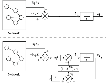
Figure 1: (Top) Without DSR: dynamics of agent $i$ for original networked system without delayed reinforcement. (Bottom) With DSR: modified dynamics of agent $i$ with delayed reinforcement using the same network information ($K_{i}Z$ and $B_{i}z_{s}$, where $B_{i}$ and $K_{i}$ are the $i^{th}$ rows of matrices $B$ and $K$).

3.5 Cohesiveness with DSR

The following lemma shows that the DSR approach leads to solutions $Z$ of Eq. (32) that are close to the ideal cohesive dynamics in Eq. (29), if either the dominant dynamics is sufficiently slow (magnitude of $\ddot{Z}$ is small) or if the delay $\tau$ is sufficiently small.

Lemma 1 (DSR and ideal cohesive dynamics).

Let the source $z_{s}$ be sufficiently smooth in a finite time interval ${\mathcal{I}_{t}}=[t_{1},t_{2}]$. Then, solutions $Z$ of the DSR Eq. (32) are close to the ideal cohesive solution $Z^{*}$ of Eq. (29), with the same synchronized initial conditions, provided the product of the time delay $\tau$ and the maximum acceleration $\ddot{Z}$ over the interval ${\mathcal{I}_{t}}$ is small. Formally, the deviation $E_{Z}=Z-Z^{*}$ satisfies

$$\max_{t\in{\mathcal{I}_{t}}}\|E_{Z}(t)\|_{\infty}\rightarrow 0,\quad{\mbox{as}}\quad\max_{t\in{\mathcal{I}_{t}}}\|\tau\ddot{Z}(t)\|_{\infty}\rightarrow 0.$$ (35)

Proof  Solutions $Z^{*}$ and $Z$ to Eqs. (29) and (32), respectively, are twice differentiable in the time interval $(t_{1},t_{2})$ if the source $z_{s}$ is sufficiently smooth. From Taylor’s theorem, given the differentiability of $Z$,

$$Z(t-\tau)=Z(t)+[-\tau]\dot{Z}(t)+\tau^{2}H(t),$$ (36)

where $H$ is bound by the maximum agent acceleration, i.e.,

$$\|H(t)\|_{\infty}~{}\leq~{}\max_{1\leq i\leq n,t\in(t_{1},t_{2})}\frac{1}{2}|\ddot{z}_{i}(t)|~{}=\overline{H}.$$ (37)

Substituting for the approximate derivative $\frac{Z(t)-Z(t-\tau)}{\tau}=\dot{Z}(t)-\tau H(t)$ in Eq. (32), and reversing the arguments from Eqs. (20) to (22), results in

$$\dot{Z}(t) =-\alpha Z(t)+{\textbf{1}}_{n}\left[\alpha z_{s}(t)+\dot{z}_{s}\right]+\frac{\tau}{\beta}K^{-1}\left[I-\beta K\right]H(t).$$ (38)

Let $Z^{*}$ be a solution to ideal cohesive dynamics in Eq. (27),

$$\dot{Z}^{*}(t) =-\alpha Z^{*}(t)+{\textbf{1}}_{n}\left[\alpha z_{s}(t)+\dot{z}_{s}\right].$$ (39)

Then, the dynamics of the deviation $E_{z}=Z-Z^{*}$ between the two solutions $Z$ and $Z^{*}$ can be found subtracting Eq. (39) from Eq. (38) to obtain

$$\dot{E}_{Z}(t) =-\alpha E_{Z}(t)+\frac{\tau}{\beta}K^{-1}\left[I-\beta K\right]H(t),$$ (40)

which is bounded-input bounded-output stable. If the initial conditions at time $t_{1}$ are the same, i.e., $E_{Z}(t_{1})=0$ then the result follows since the deviation $E_{Z}$ tends to zero as the maximum magnitude of $\tau H(t)$ (which is not bigger than $\tau\overline{H}$) tends to zero. ∎

Remark 5 (DSR cohesiveness).

From the above lemma, the use of DSR can lead to solutions close to the ideal cohesive dynamics resulting in a smaller cohesion error $\Delta^{*}$, provided the product of the maximum magnitude $\ddot{Z}$ and time delay $\tau$ is sufficiently small. However, without DSR, such a reduction is not possible for a general network. Moreover, the DSR approach (with $\beta=1$ and the derivative term $\dot{Z}$ set to zero on the right hand side of Eq. (22)) can perform as well as the case without the DSR. Therefore, in general, the use of DSR can improve cohesiveness when compared to the case without DSR.

4 Stability analysis

This section begins with a numerical check for stability, followed by conditions on the parameters ($\alpha,\beta,\tau$) for stability of the DSR approach.

4.1 Eigenvalues of pinned Laplacian $K$ and stability

With general matrices $A$, $A_{d}$ in DDE Eq. (25) it is difficult to relate the stability of the DDE to the eigenvalues of the two matrices. However, given the special structure of $A$, $A_{d}$ in the current DDE, the stability of the DDE can be related to the eigenvalues $\left\{\lambda_{K,i}\right\}_{i=1}^{n}$ of the pinned Laplacian $K$, as shown below.

Lemma 2 (Stability of DDE).

The DDE system in Eq. (25) is exponentially stable if and only if the roots $s_{i}$ of

$$s-\lambda_{i}-\lambda_{d,i}e^{-s\tau} =0$$ (41)

have negative real part, i.e.,

$${{\mathcal{R}}e\{s_{i}\}}<0$$ (42)

for all integers $1\leq i\leq n$ where

$$\lambda_{i} =-\alpha\beta\lambda_{K,i}+\frac{1}{\tau}\left[1-\beta\lambda_{K,i}\right]$$ (43)

$$\lambda_{d,i} =-\frac{1}{\tau}\left[1-\beta\lambda_{K,i}\right],$$

and $\left\{\lambda_{K,i}\right\}_{i=1}^{n}$ are eigenvalues of the pinned Laplacian $K$.

Proof  To begin, the DDE (25) is converted into a Jordan form. Let the pinned Laplacian $K$ be similar to the diagonal matrix $K_{J}$ in the Jordan form, where

$$K_{J}=P_{K}^{-1}KP_{K}$$ (44)

and the diagonal terms of matrix $K_{J}$ are the (potentially complex-valued) eigenvalues $\left\{\lambda_{K,i}\right\}_{i=1}^{n}$ of matrix $K$ [41]. Note that the multiplicity of each eigenvalue $\lambda_{K,i}$ can be more than one. The invertible (potentially complex-valued) matrix $P_{K}$ also transforms $A,A_{d}$ in the DDE Eq. (25) into Jordan-like forms $A_{J},A_{d,J}$ with (potentially complex-valued) diagonal terms $\lambda_{i},\lambda_{d,i}$ described in Eq. (43) since, from Eqs. (26) and (44),

$$A_{J}~{}~{}=P_{K}^{-1}AP_{K} =-\alpha\beta K_{J}+\frac{1}{\tau}\left[I-\beta K_{J}\right]$$ (45)

$$A_{d,J}~{}~{}=P_{K}^{-1}A_{d}P_{K} =-\frac{1}{\tau}\left[I-\beta K_{J}\right].$$

Then, setting the input $z_{s}$ to zero and changing the coordinates in the DDE Eq. (25) to $Z(t)~{}=P_{K}Z_{J}(t)$, and pre-multiplying by $P_{K}^{-1}$ on both sides results in

$$\dot{Z}_{J}(s) =A_{J}Z_{J}(s)+e^{-s\tau}A_{d,J}Z_{J}(s).$$ (46)

The stability of the DDE (25), is equivalent to the stability of the DDE (46) in the new coordinates $Z_{J}$. In particular, system is exponentially stable if the roots $s=\lambda_{DDE}$ of the characteristic equation,

$$\det\left|sI-A_{J}-A_{d,J}e^{-s\tau}\right|=0,$$ (47)

satisfy  [22, 42]

$$\sup{{\mathcal{R}}e}{(\lambda_{DDE})}<-\gamma_{\lambda}<0~{}.$$ (48)

Since $A_{J}$ and $A_{d,J}$ have triangular (Jordan) forms, the characteristic Eq. (47) can be rewritten, by considering the diagonal terms), as

$$\prod_{i=1}^{n}\left[s-\lambda_{i}-\lambda_{d,i}e^{-s\tau}\right]=0,$$ (49)

whose roots $s=\lambda_{DDE}$ are the same as roots $s_{i}$ of Eq. (41) of the lemma.

Finally, properties of analytic functions, can be used to show that roots $s_{i}$ satisfying the negative real part condition in Eq. (42) also satisfy the more stricter stability condition in Eq. (48) with $\lambda_{DDE}=s_{i}$. If the roots $\lambda_{DDE}$ have negative real parts but there is no $\gamma_{\lambda}>0$ satisfying Eq. (48), then there is an infinite number of roots $\lambda_{DDE}$ arbitrarily close to the imaginary axis ${\mathcal{R}}e\{s\}=0$. This follows by considering roots to the right of the sequence of lines ${\mathcal{R}}e\{s\}=-1/N$ that are getting closer to the imaginary axis as $N$ increases. One can find a subsequence of these lines such that there is a sequence of distinct roots to the right of each line. Note that the roots close to the imaginary axis have finite magnitude. There exists constants $\overline{s},\bar{N}$ such that there are no roots close to the imaginary axis (to the right of the line ${\mathcal{R}}e\{s\}=-1/\bar{N}$) with $|s|>\overline{s}$ because the portion of the characteristic Eq (41) is dominated by the first term $s$ and both the other terms $\lambda_{i}$ and $\lambda_{d,i}e^{-s\tau}$ are bounded on (and close to) the imaginary axis. So there are infinite roots residing in each bounded region satisfying $|s|\leq\overline{s}$ and ${\mathcal{R}}e\{s\}>-1/N$, which is not possible since Eq. (41) is analytic and can only have a finite number of zeros in any bounded region.

The necessity of the negative-real-part condition in Eq. (42) follows since the DDE has solutions with terms of the form $e^{s_{i}t}Z_{s,i}$, where $Z_{s,i}$ is the eigenvector associated with eigenvalue $s_{i}$. ∎

4.2 Numerical check for stability

Stability of the DSR could be checked numerically. For example, the roots of the characteristic Eq. (49) are composed of the roots $s_{i}$ in Eq. (41) of the individual terms forming the product in the characteristic Eq. (49), i.e., solutions to $s_{i}-\lambda_{i}-\lambda_{d,i}e^{-s_{i}\tau}=0$. The portion of the characteristic equation associated with each eigenvalue $\lambda_{K,i}$, i.e., Eq. (41), can be rewritten as

$$\tau(s_{i}-\lambda_{i})e^{\tau(s_{i}-\lambda_{i})} =\tau\lambda_{d,i}e^{-\lambda_{i}\tau},$$ (50)

which can be solved numerically using the Lambert W function [24] $W(H)e^{W(H)}=H$ as

$$s_{i,\hat{k}} =\lambda_{i}+\frac{1}{\tau}W_{\hat{k}}\left(\tau\lambda_{d,i}e^{-\lambda_{i}\tau}\right)$$ (51)

for the $\hat{k}^{th}$ branch of the Lambert W function. Solutions to the nonhomogeneous DDE (25) with nonzero source $z_{s}(t)$ can be specified using the roots in Eq. (51), especially since matrices $A$ and $A_{d}$ commute, e.g., see [25]. However, such numerical methods do not lead to a stability guarantee, which is addressed in the following subsection.

4.3 Condition for DSR stability

A condition for stability of the DDE in Eq. (25) is developed below, under the following assumption.

Assumption 2 (Selection of controller).

The DSR parameter $\beta>0$ is chosen to be sufficiently large, i.e.,

$$\beta>\max_{1\leq i\leq n}\frac{1}{{{\mathcal{R}}e}\left\{{\lambda_{K,i}}\right\}}>0,$$ (52)

where $\left\{\lambda_{K,i}\right\}_{i=1}^{n}$ are the (potentially repeated) eigenvalues of matrix $K$ with positive real parts. ∎

Theorem 1 (Exponentially stability).

Under Assumptions 1 and 2, the DDE system in Eq. (25) is exponentially stable, if

$$\left|\beta\lambda_{K,i}-1\right|-\left(\beta{{\mathcal{R}}e}\left\{{\lambda_{K,i}}\right\}-1\right) <\alpha{\tau}{{\mathcal{R}}e}\left\{{\beta\lambda_{K,i}}\right\}$$ (53)

for all eigenvalues $\left\{\lambda_{K,i}\right\}_{i=1}^{n}$ of matrix $K$.

Proof  The proof aims to show that all roots of the characteristic Eq. (49) have negative real parts (lie to the left of the imaginary axis of the complex plane) and then stability follows from Lemma 2. The proof is through contradiction. Assume that there is a root $s_{i}=a_{i}+jb_{i}$ with nonnegative real part

$${{\mathcal{R}}e\{s_{i}\}}={{\mathcal{R}}e\{a_{i}+jb_{i}\}}=a_{i}\geq 0$$ (54)

that satisfies the characteristic Eq. (49), e.g.,

$$s_{i}+\alpha\beta\lambda_{K,i}-\frac{1}{\tau}\left[1-\beta\lambda_{K,i}\right]\left(1-e^{-s_{i}\tau}\right)=0$$ (55)

for some eigenvalue $\lambda_{K,i}$ of the pinned Laplacian $K$. Then, from the nonnegative real part assumption ${{\mathcal{R}}e}\left\{{s_{i}}\right\}\geq 0$ in Eq. (54) and from Eq. (55)

$${{\mathcal{R}}e}\left\{{-\alpha\beta\tau\lambda_{K,i}+\left[1-\beta\lambda_{K,i}\right]\left(1-e^{-s_{i}\tau}\right)}\right\}\geq 0.$$ (56)

Note that the set of points defined by the second term $S_{i}(s)$,

$$S_{i}(s)~{}=\left[1-\beta\lambda_{K,i}\right]\left(1-e^{-s\tau}\right),$$ (57)

where $s$ has nonnegative real part, is bounded by the circle found by evaluating $S_{i}(s)$ on the imaginary axis. The circle is centered at $C_{i}=1-\beta\lambda_{K,i}$ and its radius ${\rho}_{i}$ is given by the magnitude of $C_{i}$, i.e., ${\rho}_{i}=|C_{i}|=|1-\beta\lambda_{K,i}|>0$.

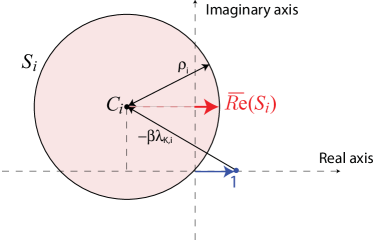
Figure 2: Set $S_{i}(s)$ in Eq. (57) when $s$ has nonnegative real part

Therefore, the maximum real part of $S_{i}(s)$ is achieved on the imaginary axis, i.e.,

$$\max_{{{\mathcal{R}}e}\left\{{s}\right\}\geq 0}{{\mathcal{R}}e}\left\{S_{i}(s)\right\}~{}~{}=\max_{{{\mathcal{R}}e}\left\{{s}\right\}=0}{{\mathcal{R}}e}\left\{S_{i}(s)\right\}.$$ (58)

Note that the real part of the center $C_{i}$ is negative

$${{\mathcal{R}}e}\left\{{C_{i}}\right\}~{}={{\mathcal{R}}e}\left\{{1-\beta\lambda_{K,i}}\right\}~{}=1-\beta{{\mathcal{R}}e}\left\{{\lambda_{K,i}}\right\}<0$$

from Assumption 2. Therefore, the maximum real part of $S_{i}(s)$ (for $s$ with nonnegative real part) is given by

$$\overline{{{\mathcal{R}}e}}\left(S_{i}\right)~{} =\max_{{{\mathcal{R}}e}\left\{{s}\right\}\geq 0}{{\mathcal{R}}e}\left\{S_{i}(s)\right\}=~{}\left|{\rho}_{i}\right|-\left|{{\mathcal{R}}e}\left\{{C_{i}}\right\}\right|$$

$$=\left|1-\beta\lambda_{K,i}\right|-\left(\beta{{\mathcal{R}}e}\left\{{\lambda_{K,i}}\right\}-1\right).$$ (59)

From Eq. (56) and Eq. (59), the assumption that the real part of the root $s_{i}$ is nonnegative implies that

$$-\alpha\beta\tau{{\mathcal{R}}e}\left\{{\lambda_{K,i}}\right\}+{{\mathcal{R}}e}\left\{{S_{i}(s_{i})}\right\} \geq 0$$ (60)

or

$${{\mathcal{R}}e}\left\{{S_{i}(s_{i})}\right\} \geq\alpha\beta\tau{{\mathcal{R}}e}\left\{{\lambda_{K,i}}\right\}.$$ (61)

This requires the maximum possible value of $S_{i}(s)$ with positive real parts to be larger than the right hand side, i.e.,

$$\max_{{{\mathcal{R}}e}\left\{{s}\right\}\geq 0}{{\mathcal{R}}e}\left\{S_{i}(s)\right\} \geq\alpha\beta\tau{{\mathcal{R}}e}\left\{{\lambda_{K,i}}\right\}$$ (62)

or

$$\left|1-\beta\lambda_{K,i}\right|-\left(\beta{{\mathcal{R}}e}\left\{{\lambda_{K,i}}\right\}-1\right) \geq\alpha\beta\tau{{\mathcal{R}}e}\left\{{\lambda_{K,i}}\right\},$$ (63)

which contradicts the condition in Eq. (53).           ∎

The stability condition in Theorem 1 can be restated in terms of the known range of the eigenvalues $\lambda_{K,i}$ of the pinned Laplacian $K$ .

Assumption 3 (Range of eigenvalues).

The eigenvalues $\lambda_{K,i}=m_{i}e^{j\phi_{i}},$ lie in the range specified by

$$0 <\underline{m}\leq m_{i}\leq\overline{m},\quad~{}|\phi_{i}|\leq\overline{\phi}<\frac{\pi}{2},$$ (64)

where the zero lower bound on the magnitude $m_{i}$ and the upper bound $\frac{\pi}{2}$ on the phase $\phi_{i}$ arise since the eigenvalues $\lambda_{K,i}$ have positive real parts, as in Eq. (10). ∎

Corollary 4.1 (Range-based stability).

Under Assumptions 2 and 3, the stability condition in Eq. (53) of Theorem 1 is met if

$$\frac{\overline{\rho}~{}+1}{\overline{\rho}\cos{\overline{\psi}}~{}+1}-1<\alpha{\tau}$$ (65)

where, with $\beta{\underline{m}\cos{\overline{\phi}}}>1$ to satisfy Assumption 2,

$$\overline{\rho} =\sqrt{\left(\beta\overline{m}\sin{\overline{\phi}}\right)^{2}+\left(\beta\overline{m}\cos{\overline{\phi}}-1\right)^{2}}$$ (66)

$$\overline{\psi} =\tan^{-1}\left(\frac{\beta\underline{m}\sin{\overline{\phi}}}{\beta\underline{m}\cos{\overline{\phi}}-1}\right).$$

Proof  Note that the real part of $\beta\lambda_{K,i}$ is greater than one from Eq. (52). Let $|\beta\lambda_{K,i}-1|={\rho}_{i}$, and $\beta{{\mathcal{R}}e}\left\{{\lambda_{K,i}}\right\}-1={\rho}_{i}\cos{\psi_{i}}$ as in Fig. 3.

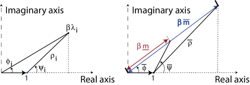
Figure 3: (Left) Stability condition terms in Eq. (67) for a specific eigenvalue $\lambda_{i}$. (Right) Terms in Eq. (65) based on range of eigenvalue $\lambda_{i}$ in Assumption 3.

Therefore, the stability condition in Eq. (53) can be rewritten as

$$\frac{{\rho}_{i}-{\rho}_{i}\cos{\psi_{i}}}{{\rho}_{i}\cos{\psi_{i}}+1}~{}=\frac{{\rho}_{i}+1}{{\rho}_{i}\cos{\psi_{i}}+1}-1~{} <\alpha{\tau},$$ (67)

where the left hand side (lhs) of the inequality is a monotonic (nondecreasing) function of each variable $\rho_{i}$ and $\psi_{i}$, independent of the other variable, over the entire interval ${\rho}_{i}>0$ and $0\leq\psi_{i}<\pi/2$, since

$$\frac{\partial}{\partial{\rho}_{i}}\left(\frac{{\rho}_{i}+1}{{\rho}_{i}\cos{\psi_{i}}+1}\right) =\frac{1-\cos{\psi_{i}}}{\left({\rho}_{i}\cos{\psi_{i}}+1\right)^{2}}~{}~{}\geq 0,$$ (68)

$$\frac{\partial}{\partial{\psi}_{i}}\left(\frac{{\rho}_{i}+1}{{\rho}_{i}\cos{\psi_{i}}+1}\right) =\frac{({\rho}_{i}+1){\rho}_{i}\sin{\psi_{i}}}{\left({\rho}_{i}\cos{\psi_{i}}+1\right)^{2}}~{}~{}\geq 0.$$

Due to symmetry, only the top portion of the right-half plane is considered, i.e., $0\leq\phi_{i}$, $0\leq\psi_{i}<\pi/2$. Therefore, the lhs of Eq. (67) is maximized with the largest selection of ${\rho}_{i}$ and $\psi_{i}$. The largest angle $\psi_{i}$ is $\overline{\psi}$ as in Eq. (66) corresponding to the smallest magnitude $\underline{m}$ and largest phase $\overline{\phi}$ in the range specified by Eq. (64) since the derivative of

$$\tan{\psi_{i}}=\beta m_{i}\sin{\phi_{i}}/\left(\beta m_{i}\cos{\phi_{i}}-1\right)$$ (69)

is nonpositive with respect to the magnitude $m_{i}$ and nonnegative with respect to phase $0\leq\phi_{i}<\overline{\phi}$ of the eigenvalue $\lambda_{K,i}$ satisfying Eq. (64),

$$\frac{\partial\tan{\psi_{i}}}{\partial m_{i}} =\frac{-\beta\sin{\phi_{i}}}{\left({\beta{m_{i}}\cos{\phi_{i}}-1}\right)^{2}}~{}~{}\leq 0,$$ (70)

$$\frac{\partial\tan{\psi_{i}}}{\partial\phi_{i}} =\frac{\beta m_{i}(\beta m_{i}-\cos{\phi_{i}})}{\left({\beta{m_{i}}\cos{\phi_{i}}-1}\right)^{2}}~{}~{}\geq 0$$

as $\beta m_{i}\geq\beta m_{i}\cos{\phi_{i}}>1\geq\cos{\phi_{i}}$ from Eq. (52). Similarly, the largest magnitude ${\rho}_{i}$ is $\overline{\rho}$ is obtained by choosing the largest magnitude $\overline{m}$ and largest phase $\overline{\phi}$ for the eigenvalues $\lambda_{K,i}$ satisfying Eq. (64), as in Eq. (66). This is because the derivative of the square of the magnitude

$${\rho}_{i}^{2} =(\beta m_{i}\sin{(\phi_{i})})^{2}+(\beta m_{i}\cos{(\phi_{i})}-1)^{2}$$ (71)

$$=\beta^{2}m_{i}^{2}-2\beta m_{i}\cos{(\phi_{i})}+1$$

is a nondecreasing function of magnitude $m_{i}>0$ and phase $\phi_{i}$, with $0<\phi_{i}\leq\pi/2$, since

$$\frac{\partial{\rho_{i}}^{2}}{\partial m_{i}} =2\beta^{2}m_{i}-2\beta\cos{(\phi_{i})}=2\beta\left(\beta m_{i}-\cos{(\phi_{i})}\right)\geq 0$$ (72)

$$\frac{\partial{\rho_{i}}^{2}}{\partial\phi_{i}} =2\beta m_{i}\sin{(\phi_{i})}~{}~{}\geq 0.$$

The theorem follows since the lhs of Eq. (65) is an upper bound for the lhs of Eq. (67) ∎

4.4 Topological ordering and rapid cohesive transition

Arbitrarily-fast cohesive transition can be achieved (within constraints, such as actuator bandwidth) if the eigenvalues of the pinned Laplacian $K$ are real, as shown below. Additionally, this section connects the stability analysis of the proposed DSR approach in Theorem 1 with prior methods for stability of DDEs.

With real eigenvalues $\lambda_{K,i}$, the only condition for stability is that the parameter $\beta$ be sufficiently large, as in Assumption 2. This is stated formally below.

Corollary 4.2 (Response rate with real eigenvalues).

Let the eigenvalues $\lambda_{K,i}$ of the pinned Laplacian $K$ be real, i.e., ${{\mathcal{R}}e}\left\{{\lambda_{K,i}}\right\}=\lambda_{K,i}$ for all $1\leq i\leq n$ and let the parameter $\beta$ be sufficiently large as in Eq. (52). Then, the system with DSR is stable for any positive choice of the cohesive response rate $\alpha>0$ and the time delay $\tau>0$.

Proof  With real eigenvalues $\lambda_{K,i}$, from Assumption 2,

$$\left|\beta\lambda_{K,i}-1\right|=\beta\lambda_{K,i}-1,\qquad\left(\beta{{\mathcal{R}}e}\left\{{\lambda_{K,i}}\right\}-1\right)=\beta\lambda_{K,i}-1.$$

Therefore, the condition in Eq. (53) of Theorem 1 becomes $0<\alpha{\tau}\beta\lambda_{K,i}$, which is satisfied for any positive response-rate parameter $\alpha$ and delay $\tau$ since $\beta>0$ and $\lambda_{K,i}>0$. ∎

Remark 6 (Undirected graph).

Using Theorem 1 in [32], it can be shown that the DDE in Eq. (25) is stable when the graph ${\mathcal{G}}\!\setminus\!s$ associated with the pinned Laplacian $K$ is undirected, provided $-A\pm A_{d}$ is positive definite. The positive definiteness of $-A\pm A_{d}$ follows from Corollary 4.2 when $\alpha>0,\beta>0$. Note that $-A-A_{d}=\alpha\beta K$ is positive definite since $K$ is positive definite. Moreover, $-A+A_{d}=\alpha\beta K-\frac{2}{\tau}\left[I-\beta K\right]$ is positive definite since it is symmetric and its eigenvalues $\lambda_{AAd}$ are positive, i.e., $\lambda_{AAd}=\alpha\beta\lambda_{K,i}-2\frac{1}{\tau}\left[1-\beta\lambda_{K,i}\right]>0$ since $\lambda_{K,i}>0$ are the positive eigenvalues of the symmetric pinned Laplacian $K$ and $\lambda_{K,i}\beta>1$ from Assumption 2.

Remark 7 (Necessary and sufficient conditions).

The conditions of Corollary 4.2 meet the following necessary and sufficient conditions for stability developed in [33] (when the parameters of the characteristic equation $\lambda_{i},\lambda_{d,i}$ are real), i.e.,

$$\lambda_{i}<1,\quad{\mbox{and}}\quad\lambda_{i}<-\lambda_{d,i}<(V_{\lambda}^{2}+\lambda_{i}^{2})^{\frac{1}{2}},$$ (73)

where $V_{\lambda}$ is the root of $V_{\lambda}\cot{V_{\lambda}}=\lambda_{i}$ such that $0<V_{\lambda}<\pi$. Note that $\lambda_{i}$ from Eq. (43) becomes

$$\lambda_{i}=-\alpha\beta\lambda_{K,i}+\frac{1}{\tau}\left[1-\beta\lambda_{K,i}\right],$$

which is less than zero since $\beta\lambda_{K,i}>1$ and each term in $\alpha\beta\lambda_{K,i}$ is positive. Moreover, $\lambda_{i}<-\lambda_{d,i}$ from the definition in Eq. (43) since the terms $\alpha\beta\lambda_{K,i}>0$, and $-\lambda_{d,i}<(V_{\lambda}^{2}+\lambda_{i}^{2})^{\frac{1}{2}}$ since $|\lambda_{i}|>|\lambda_{d,i}|$ and $V_{\lambda}>0$. ∎

When the pinned Laplacian $K$ associated with the graph ${\mathcal{G}}\!\setminus\!s$ of the non-source agents is undirected, the pinned Laplacian $K$ is real symmetric and therefore its eigenvalues are real. However, the eigenvalues of the pinned Laplacian $K$ can be real with directed graphs such as topologically-ordered subgraphs.

Remark 8 (Topologically ordered graphs).

For acyclic directed graphs (or topologically ordered graphs), the pinned Laplacian $K$ will be lower-diagonal and hence have real eigenvalues. In an acyclic graph there is a topological ordering of the nodes ${\mathcal{V}}$ and every graph edge ${\mathcal{E}}$ goes from a node that is earlier in the ordering to a node that is later in the ordering, i.e., all the neighbors $N_{i}$ of a node $i$ are earlier in the ordering. This leads to a pinned Laplacian $K$ which is lower diagonal and real and hence, with real eigenvalues. ∎

Remark 9 (Topologically-ordered sub-graphs).

The eigenvalues of the pinned Laplacian $K$ are real when the matrix $K$ is associated with a set of subgraphs ${\mathcal{G}}_{i}$ that are distinct (i.e., without shared nodes) where each subgraph is either symmetric or acyclic (topologically ordered) with an additional topological ordering of the subgraphs ${\mathcal{G}}_{i}$ such that all graph edges in ${\mathcal{G}}\!\setminus\!s$ ends in one of the subgraphs, say ${\mathcal{G}}_{i}$ and starts: (a) either in the same ending subgraph ${\mathcal{G}}_{i}$; or (b) in a subgraph that is earlier than the ending subgraph ${\mathcal{G}}_{i}$ in the subgraph ordering. Such topological ordering of the subgraphs ensures that the pinned Laplacian $K$, associated with the graph ${\mathcal{G}}\!\setminus\!s=\bigcup{\mathcal{G}}_{i}$ is lower block-diagonal with symmetric matrices $K_{i}$ in each diagonal block. Then, the eigenvalues of the pinned Laplacian $K$ are real because they are the same as the eigenvalues of the real-valued matrices $K_{i}$, each of which is either diagonal or symmetric. ∎

Remark 10 (Impact of noise).

Although stability is not impacted by the noise, the cohesion performance can deteriorate in the presence of substantial noise. If noise of size $N_{v}$ is present in the estimation of $v$ in Eq. (34), then it leads to a noise of order $\frac{N_{v}}{\tau}$ due to the approximated derivative in Eq. (33). Thus, the time delay $\tau$ needs to be sufficiently large to reduce the noise effect on the dynamics, which in turn increases the achievable settling time $T_{s}$ as in Eq. (24). Alternatively, the noise can be filtered as shown in the following subsection.

4.5 DSR with higher-order dynamics

The DSR approach can be extended to enable cohesive tracking when the agents have higher-order dynamics, and the DSR update can be filtered to reduce noise effects, as shown below.

4.5.1 Agent’s higher-order dynamics

Let the dynamics of an individual agent $i$ be given by a minimum-phase system in the output-tracking form (through appropriate input and state transformations, e.g., see [43]) as

$${z}_{i}^{(r)}(t) =u_{i}(t),$$ (74)

$$\frac{d}{dt}{\eta}_{i}(t) =A_{\eta,i}{\eta}_{i}(t)+A_{z,i}Z_{i}(t),$$

where $r$ is the relative degree (i.e., the difference between the number of poles and the number of zeros), the bracketed superscript denotes the time derivative, e.g., $z_{i}^{(r)}$ represents the $r^{th}$ time derivative of $z_{i}$, and $Z_{i}$ represents the agent output $z_{i}$ and its time derivatives $z_{i}^{(k)}$, $1\leq k\leq r-1$. The internal dynamics represented by $\eta_{i}$ is stable, i.e., $A_{\eta,i}$ is Hurwtiz, since the system is minimum phase. Note that the stability of the internal dynamics is independent of the selection of the control input $u_{i}$.

Remark 11 (Heterogeneous agents).

The internal dynamics ${\eta}_{i}$ in Eq. (74) can be different and can be nonlinear, provided the dynamics remain close to the stable origin of the internal dynamics. In this sense, the approach is applicable to heterogeneous agents.

Assumption 4 (Relative degree).

All agents have minimum-phase dynamics and the same well-defined relative degree $1\leq r\leq n$. ∎

4.5.2 Ideal cohesive higher-order dynamics

If each non-source agent can have instantaneous access to the source $z_{s}$ (which is sufficiently smooth), then the input $u_{i}(t)$ can be selected such that the output $z_{i}$ dynamics is given by, as in Eq. (18),

$${z}_{i}^{(r)}(t) ={z}_{s}^{(r)}(t)-\sum_{k=0}^{r-1}\hat{\alpha}_{k}\left({z}_{i}^{(k)}(t)-{z}_{s}^{(k)}(t)\right).$$ (75)

With the same initial condition, the response of all the agents would track the desired output $z_{s}$ in a cohesive manner. The output tracking is stable since the characteristic equation ${\mathcal{P}}(s)=0$,

$${\mathcal{P}}(s)=\sum_{k=0}^{r}\hat{\alpha}_{k}s^{k}=(s+\alpha)^{r}$$ (76)

has stable roots provided $\alpha>0$. Note that the leading coefficient is one, i.e., $\hat{\alpha}_{r}=1$, and the constant $\alpha$ can be varied to adjust the overall speed of the response of each agent. In a vector form, this ideal cohesive dynamics can be written as

$${Z}^{(r)}(t) =-\sum_{k=0}^{r-1}\hat{\alpha}_{k}{Z}^{(k)}(t)+{\textbf{1}}_{n}\sum_{k=0}^{r}\hat{\alpha}_{k}{z}_{s}^{(k)}(t).$$ (77)

Multiplying both sides of Eq. (77) by $\beta K$ (where $\beta>0$) and using Eq. (11) to replace $K{\textbf{1}}_{n}$ results in

$$\beta K{Z}^{(r)}(t) =-\beta K\sum_{k=0}^{r-1}\hat{\alpha}_{k}{Z}^{(k)}(t)+\beta Bz_{s}^{*}(t),$$ (78)

where $z_{s}^{*}(t)=\sum_{k=0}^{r}\hat{\alpha}_{k}{z}_{s}^{(k)}(t)$. By adding ${Z}^{(r)}$ on both sides of Eq. (78), the ideal cohesive dynamics can be rewritten as

$${Z}^{(r)}(t) =-\beta K\sum_{k=0}^{r-1}\hat{\alpha}_{k}{Z}^{(k)}(t)+\beta Bz_{s}^{*}(t)+\left[I-\beta K\right]{Z}^{(r)}(t).$$ (79)

4.5.3 DSR-based implementation

Approximating the derivative ${Z}^{(r)}$ on the right hand side of Eq. (79) in terms of delayed versions of the system state, as in Eq. (23),

$${Z}^{(r)}(s) \approx\hat{Z}^{(r)}(s,\tau)=\left[f(s)\frac{1-e^{-\tau s}}{\tau}\right]^{r}Z(s)={\mathcal{F}}(s)Z(s),$$ (80)

where $f(s)$ is a low-pass filter, yields the DSR approach for networks with higher-order dynamics. Replacing ${Z}^{(r)}(t)$ with $\hat{Z}^{(r)}(t,\tau)$, the Laplace inverse of $\hat{Z}^{(r)}(s,\tau)$, Eq. (79) becomes

$${Z}^{(r)}(t) =-\beta K\sum_{k=0}^{r-1}\hat{\alpha}_{k}{Z}^{(k)}(t)+\beta Bz_{s}^{*}(t)+\left[I-\beta K\right]\hat{Z}^{(r)}(t,\tau).$$ (81)

As in the first-order case, the DSR-based extension for the case when agents have higher-order dynamics only uses local information from the neighbors and does not require network changes.

4.6 Stability of DSR approach

Stability of the DSR approach in Eq. (81) depends on the roots of the characteristic equation

$$\det\left|s^{r}I+\beta K\sum_{k=0}^{r-1}\hat{\alpha}_{k}s^{k}-\left(I-\beta K\right){\mathcal{F}}(s)\right|=0.$$ (82)

In particular, using arguments similar to those in Lemma 2, the DSR-based approach is stable if and only if the roots $s_{i}$ of

$$s^{r}+\beta\lambda_{K,i}\sum_{k=0}^{r-1}\hat{\alpha}_{k}s^{k}-\left(1-\beta\lambda_{K,i}\right){\mathcal{F}}(s)=0$$ (83)

have negative real part where $\left\{\lambda_{K,i}\right\}_{i=1}^{n}$ are eigenvalues of the pinned Laplacian $K$. Equation (83) can be rewritten using Eq. (76) as

$$(1-\beta\lambda_{K,i})s^{r}+\beta\lambda_{K,i}{\mathcal{P}}(s) -\left(1-\beta\lambda_{K,i}\right){\mathcal{F}}(s)=0$$

or, since $1-\beta\lambda_{K,i}\neq 0$ under Assumption 2,

$$s^{r} +\frac{\beta\lambda_{K,i}}{(1-\beta\lambda_{K,i})}{\mathcal{P}}(s)={\mathcal{F}}(s).$$ (84)

Theorem 2 (Exponentially stability of extended DSR).

Under Assumptions 1-4, the origin $Z(t)=0$ of the DDE system in Eq. (81) is exponentially stable, if

$$\sup_{{\mathcal{R}}e(s)\geq 0}\left|f(s)\left(1-e^{-\tau s}\right)\right| <\left(\epsilon_{\lambda}\right)^{\frac{1}{r}}\alpha\tau,$$ (85)

where

$$\epsilon_{\lambda} =\frac{\beta{\overline{m}}}{\sqrt{\beta^{2}\overline{m}^{2}-2\beta\overline{m}\cos{\overline{\phi}}+1}}\quad~{}{\mbox{if}}~{}r>1$$ (86)

$$=\frac{\beta{\underline{m}}\cos{\overline{\phi}}}{\sqrt{\beta^{2}\overline{m}^{2}-2\beta\overline{m}\cos{\overline{\phi}}+1}}\quad~{}{\mbox{if}}~{}r=1$$ (87)

Proof  This is shown by contradiction. Assume that $s_{i}=a_{i}+jb_{i}$ is a root of Eq. (84) with nonnegative real part $a_{i}\geq 0$. Then, with $s=s_{i}$, it is shown below that, under the theorem’s condition, that the smallest magnitude of the right hand side (rhs) of Eq. (84) is greater than the largest magnitude of the left hand side (lhs), which contradicts the assumption that $s_{i}$ is a root of Eq. (84).

First, the case when the relative degree $r\geq 2$ is considered. Consider the magnitude of the factor multiplying ${\mathcal{P}}(s)$ in Eq. (84). Note that, for any eigenvalue $\lambda_{K,i}$ of the pinned Laplacian $K$ satisfying Assumption 2, $0<\beta m_{i}\cos{\phi_{i}}-1<\beta m_{i}\cos{\phi_{i}},$ and therefore

$$\left|\frac{\beta\lambda_{K,i}}{(1-\beta\lambda_{K,i})}\right| =\frac{\sqrt{(\beta m_{i}\cos{\phi_{i}})^{2}+(\beta m_{i}\sin{\phi_{i}})^{2}}}{\sqrt{(\beta m_{i}\cos{\phi_{i}}-1)^{2}+(\beta m_{i}\sin{\phi_{i}})^{2}}}>1$$ (88)

for all magnitude $m_{i}$ and phase $\phi_{i}$ satisfying Assumption 3. The square of lhs of the inequality is monotonic non-increasing with both magnitude $m_{i}>0$ and phase $0\leq\phi_{i}<\overline{\phi}$ since

$$\frac{\partial}{\partial m_{i}}\left|\frac{\beta\lambda_{K,i}}{(1-\beta\lambda_{K,i})}\right|^{2} =\frac{-2\beta^{2}m_{i}\left(\beta m_{i}\cos{\phi_{i}}-1\right)}{\left|1-\beta\lambda_{K,i}\right|^{4}}\leq 0,$$ (89)

$$\frac{\partial}{\partial\phi_{i}}\left|\frac{\beta\lambda_{K,i}}{(1-\beta\lambda_{K,i})}\right|^{2} =\frac{-2\beta^{3}m_{i}^{3}\sin{\phi_{i}}}{\left|1-\beta\lambda_{K,i}\right|^{4}}\leq 0.$$

Therefore, from Eqs. (64), (88) and (89),

$$\left|\frac{\beta\lambda_{K,i}}{(1-\beta\lambda_{K,i})}\right|\geq\frac{\beta{\overline{m}}}{\sqrt{\beta^{2}\overline{m}^{2}-2\beta\overline{m}\cos{\overline{\phi}}+1}}=\epsilon_{\lambda}>1,$$ (90)

and

$$\left|\frac{\beta\lambda_{K,i}}{(1-\beta\lambda_{K,i})}{\mathcal{P}}(s_{i})\right|=\left|\frac{\beta\lambda_{K,i}}{(1-\beta\lambda_{K,i})}\right|\left|{\mathcal{P}}(s_{i})\right| \geq\epsilon_{\lambda}\left|{\mathcal{P}}(s_{i})\right|.$$ (91)

Moreover, for any root $s_{i}=a_{i}+jb_{i}$ with nonnegative real part $a_{i}\geq 0$, since $\alpha>0$ in Eq. (76) for stable cohesive tracking,

$$|s_{i}+\alpha|^{k}=\left[\left(a_{i}+\alpha\right)^{2}+b_{i}^{2}\right]^{k/2}>\left[a_{i}^{2}+b_{i}^{2}\right]^{k/2}=|s_{i}|^{k}\geq 0,$$

for all integers $k\geq 0$. Therefore,

$$\left|{\mathcal{P}}(s_{i})\right|=|s_{i}+\alpha|^{r}>\left|s_{i}\right|^{r}$$ (92)

and since $\epsilon_{\lambda}>1$ from Eq. (90), from Eq. (91) and (92),

$$\left|s_{i}^{r}+\frac{\beta\lambda_{K,i}}{(1-\beta\lambda_{K,i})}{\mathcal{P}}(s_{i})\right| \geq\epsilon_{\lambda}|s_{i}+\alpha|^{r}-\left|s_{i}\right|^{r}>0.$$ (93)

To find the smallest possible magnitude of the lhs of Eq. (84), the difference in magnitudes of its two terms, i.e., the rhs of Eq. (93), is compared below. Note that the difference $H(s_{i},k)$

$$H(s_{i},k)=\epsilon_{\lambda}|s_{i}+\alpha|^{k}-|s_{i}|^{k}~{}~{}>0$$ (94)

is positive for all $k\geq 0$. Moreover, the difference $H(s_{i},r)$, between the magnitudes of the terms in the lhs of Eq. (84), is also a monotonic (non-decreasing) function with the components $a_{i}\geq 0$ and $b_{i}^{2}\geq 0$ of the root $s_{i}$, since

$$\frac{\partial H(s_{i},r)}{\partial b_{i}^{2}} =\frac{r\epsilon_{\lambda}}{2}\left|(a_{i}+\alpha)^{2}+b_{i}^{2}\right|^{\frac{r}{2}-1}-\frac{r}{2}\left|a_{i}^{2}+b_{i}^{2}\right|^{\frac{r}{2}-1}$$

$$= \frac{r}{2}\left[\epsilon_{\lambda}|s_{i}+\alpha|^{r-2}-|s_{i}|^{r-2}\right]~{}=\frac{r}{2}H(s_{i},r-2)>0,$$

$$\frac{\partial H(s_{i},r)}{\partial a_{i}} =r\left[\epsilon_{\lambda}|s_{i}+\alpha|^{r-2}-|s_{i}|^{r-2}\right]a_{i}+r\epsilon_{\lambda}|s_{i}+\alpha|^{r-2}\alpha$$

$$= ra_{i}H(s_{i},r-2)+r\alpha\epsilon_{\lambda}|s_{i}+\alpha|^{r-2}\geq r\epsilon_{\lambda}\alpha^{r-1}>0$$

when $r\geq 2$. Therefore, the magnitude difference $H(s_{i},r)$, i.e., the smallest possible magnitude on the lhs of Eq. (84) is bounded from below by (when $a_{i}=b_{i}=0$)

$$H(s_{i},r) >\epsilon_{\lambda}\alpha^{r}.$$ (95)

If this lower bound on the magnitude difference $H(s_{i},r)$ of the lhs is larger than the maximum magnitude of the rhs ${\mathcal{F}}(s)$ in Eq. (84), then $s_{i}$ cannot be a root, i.e., a contradiction is obtained if

$$\epsilon_{\lambda}\alpha^{r} >\sup_{{\mathcal{R}}e(s)\geq 0}\left|f(s)\frac{1-e^{-\tau s}}{\tau}\right|^{r},$$ (96)

which follows from the condition in Eq. (85).

Second, for the case when the relative degree is one, $r=1$, the magnitude of the lhs of Eq. (84) is given by

$$\left|s_{i}+\frac{\beta\lambda_{K,i}}{(1-\beta\lambda_{K,i})}{\mathcal{P}}(s_{i})\right| =\frac{\left|(a+jb)+\alpha\beta\lambda_{K,i}\right|}{\left|(1-\beta\lambda_{K,i})\right|}~{}~{}\geq\frac{\beta{{\mathcal{R}}e}(\lambda_{K,i})}{\left|(1-\beta\lambda_{K,i})\right|}\alpha$$ (97)

since $a\geq 0$ and real part of $\lambda_{K,i}$ is positive. Note that the numerator ${{\mathcal{R}}e}(\lambda_{K,i})$ is greater than or equal to the minimum possible value, $\underline{m}\cos{\overline{\phi}}$, and the denominator $\left|(1-\beta\lambda_{K,i})\right|$ is maximized by $\overline{\rho}$ from Eq. (66). Therefore, the rhs of Eq. (97) is bounded from below by $\epsilon_{\lambda}\alpha~{}>0$. Again, if this minimum magnitude $\epsilon_{\lambda}\alpha$ of the lhs is larger than the rhs of Eq. (84), i.e., the condition in Eq. (85) is met, then $s_{i}$ with a nonnegative real part cannot be a root of Eq. (84). ∎

Remark 12 (Impact of filter).

The filter $f(s)$ can be used to reduce the impact of noise with the delay-based approximation of the derivative in Eq. (80). Note that the expression $\left(1-e^{-\tau s}\right)$ in Condition (85) tends to zero when $s$ is small. Therefore, the use of an appropriate low pass filter (e.g., sufficiently small $\Omega$ when $f(s)=\Omega/(s+\Omega)$) can ensure that the lhs is small enough to satisfy Condition (85) for any delay $\tau$. However, aggressive filtering can reduce the effective bandwidth of the DSR-based cohesiveness.

Remark 13 (Comparison of DSR stability conditions).

For first-order agents, the stability condition Eq. (85) in Theorem 2, used to extend the DSR approach to higher-order agents (using magnitude-based arguments), is more conservative than the condition in Eq. (53) in Theorem 1 that uses real-component-based arguments for first-order agents. In particular, the lhs of in Eq. (53) of Theorem 1 is zero when the eigenvalues of the pinned Laplacian $K$ are real. In contrast, the lhs is nonzero, under the same conditions, in Eq. (85) of Theorem 2.

Remark 14 (Computational issues).

When the eigenvalues $\lambda_{K,i}$ of the pinned Laplacian $K$ are known, the lower bound $\epsilon_{\lambda}$ in Eqs. (86) and (87) can be replaced by ${\overline{\epsilon_{\lambda}}}$ computed as

$$\epsilon_{\lambda}={\overline{\epsilon_{\lambda}}}=\min_{1\leq i\leq n}\left|\frac{\beta\lambda_{K,i}}{(1-\beta\lambda_{K,i})}\right|~{}\quad~{}{\mbox{if}}~{}r>1$$ (98)

$$\epsilon_{\lambda}={\overline{\epsilon_{\lambda}}}=\min_{1\leq i\leq n}\left|\frac{\beta{{\mathcal{R}}e}(\lambda_{K,i})}{(1-\beta\lambda_{K,i})}\right|~{}\quad~{}{\mbox{if}}~{}r=1.$$ (99)

When the filter has the form $f(s)=\Omega/(s+\Omega)$ whose magnitude decreases when the real part of $s$ is positive and increasing, the lhs of the stability condition in Eq. (85) can be computed over the imaginary axis, i.e.,

$$\sup_{{\mathcal{R}}e(s)\geq 0}\left|f(s)\left(1-e^{-\tau s}\right)\right|=\sup_{{\mathcal{R}}e(s)=0}\left|f(s)\left(1-e^{-\tau s}\right)\right|.$$ (100)

5 Simulation results and discussion

Simulation results are used to (i) comparatively evaluate cohesion with and without DSR; and (ii) to show the advantages of using DSR over attempting to increase the response speed for better cohesion. While cohesion is expected to be better for smoother trajectories, the step response is used in the following to quantify the cohesion, as described at the end of Section 2.

5.1 First-order example system

Consider an example system where the graph ${\mathcal{G}}\!\setminus\!s$ is composed of an ordered set of subgraphs ${\mathcal{G}}_{1}<{\mathcal{G}}_{2}<{\mathcal{G}}_{3}$ as shown in Fig. 4, where ${\mathcal{G}}_{1}$ and ${\mathcal{G}}_{2}$ are undirected subgraphs and ${\mathcal{G}}_{3}$ is an ordered acyclic graph associated with node sets ${\mathcal{V}}_{1}=\left\{1\right\},{\mathcal{V}}_{2}=\left\{2,3\right\}$ and ordered set ${\mathcal{V}}_{3}=\left\{4<5<6\right\}$, respectively. The associated pinned Laplacian $K$, where the weights $w_{ij}$ in Eq. (5) are either $0$ or $1$, is

$$K =\left[\begin{array}[]{c|c|c}\begin{matrix}1\end{matrix}&\begin{matrix}0&0\end{matrix}&\begin{matrix}0&0&0\end{matrix}\\ \hline\cr\begin{matrix}-1\\ -1\end{matrix}&\begin{matrix}2&-1\\ -1&2\end{matrix}&\begin{matrix}0&0&0\\ 0&0&0\end{matrix}\\ \hline\cr\begin{matrix}0\\ 0\\ 0\end{matrix}&\begin{matrix}-1&0\\ 0&-1\\ -1&-1\end{matrix}&\begin{matrix}1&0&0\\ 0&1&0\\ -1&-1&4\end{matrix}\end{array}\right]=\left[\begin{array}[]{c|c|c}K_{1}&\begin{matrix}0&0\end{matrix}&\begin{matrix}0&0&0\end{matrix}\\ \hline\cr\begin{matrix}-1\\ -1\end{matrix}&K_{2}&\begin{matrix}0&0&0\\ 0&0&0\end{matrix}\\ \hline\cr\begin{matrix}0\\ 0\\ 0\end{matrix}&\begin{matrix}-1&0\\ 0&-1\\ -1&-1\end{matrix}&K_{3}\end{array}\right].$$ (107)

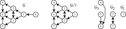
Figure 4: Network example used in simulations consisting of topologically ordered subgraphs ${\mathcal{G}}_{1}<{\mathcal{G}}_{2}<{\mathcal{G}}_{3}$ of graph ${\mathcal{G}}\!\setminus\!s$ composed of undirected subgraphs ${\mathcal{G}}_{1}$, ${\mathcal{G}}_{2}$ and directed acyclic graph ${\mathcal{G}}_{3}$ associated with node sets ${\mathcal{V}}_{1}=\left\{1\right\},{\mathcal{V}}_{2}=\left\{2,3\right\}$ and ordered set ${\mathcal{V}}_{3}=\left\{4<5<6\right\}$, respectively. All edges in graph ${\mathcal{G}}\!\setminus\!s$ that ends in one of the subgraphs, say ${\mathcal{G}}_{i}$, starts: (a) either in the same subgraph ${\mathcal{G}}_{i}$; or (b) in a subgraph that is earlier than the subgraph ${\mathcal{G}}_{i}$ in the subgraph ordering.

The eigenvalues of the pinned Laplacian $K$ are then the eigenvalue $1$ of $K_{1}$, eigenvalues $1,3$ of $K_{2}$ and eigenvalues $1,1,4$ of $K_{3}$ for the example in Fig. 4.

5.2 Step response without DSR

To illustrate the cohesion problem, the step response of the nominal system without DSR in Eq. (6) with zero as initial condition is shown in Fig. 5 where the the source $z_{s}$ is a unit step. Due to symmetry, and same initial conditions, states 2 and 3 are similar, and so are states 4 and 5, and hence there are four distinct plots in the step response. The loss of cohesion is visually observable in Fig. 5 as differences between the different agent responses, and can be quantified as deviation $\Delta=3.73$ in Eq. (15). The settling time $T_{s}$ to 2% of the final value is $T_{s}=7.5$ s. The normalized deviation is $\Delta^{*}=0.496$, as in Eq. (17).

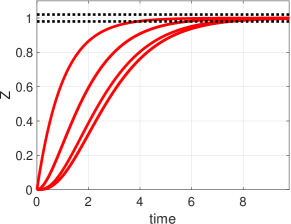
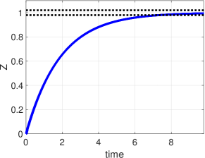
Figure 5: Step response $Z$ with first-order agents. (Left) Deviation from cohesion in step response of the nominal system without DSR in Eq. (6). (Right) Cohesive response with DSR as in Eq. (25), with similar settling time $T_{s}$.

5.3 Improved cohesion with DSR

The improvement in cohesion with DSR is evaluated when the response speed is similar to the case without DSR. Hence the parameter $\alpha$ is selected to yield a similar settling time $T_{s}=7.5$ s as in Fig. 5 for the case without DSR, i.e., from Eq. (19), $\alpha=0.53$. Moreover, the delay $\tau$ is chosen to be a hundred times smaller than the settling time $T_{s}$ as in Remark 2, i.e., $\tau=T_{s}/100=0.075$ s. Since the eigenvalues of the pinned Laplacian $K$ are real, the DSR-based approach is stable if the parameter $\beta$ is chosen to be larger than the inverse of smallest eigenvalue magnitude (which is one for this example), i.e., to satisfy Eq. (52) in Assumption 2, the parameter $\beta$ needs to be larger than one and is selected as $\beta=2$. Then, with these choices of parameters ($\alpha,\beta,\tau$), the roots $s_{i,\hat{k}}$ of the characteristic equation associated with the DDE in Eq. (25), found using the Lambert W function as in Eq. (51), are all in the left half of the complex plane as seen in Fig. 6, and thereby, confirming the expected stability of the DDE.

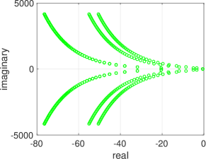
Figure 6: DDE in Eq. (25) is stable since the roots of its characteristic equation, found from Eq. (25), are in the open left-half of the complex plane.

Substantial improvement in cohesion of the step response of the system with DSR in Eq. (25) is seen in Fig. 5. The cohesion deviation $\Delta$ in Eq. (15) has reduced by $77.5$ times from $\Delta=3.72$ without DSR to $\Delta=0.048$ with DSR. The settling time to 2% of the final value is similar, i.e., $T_{s}=7.4$ s, and the normalized deviation $\Delta^{*}$ in Eq. (17) also reduces substantially (by 76 times) to $\Delta^{*}=0.0065$. Thus, the use of DSR results in substantial improvements in the cohesion.

5.4 Cohesive versus rapid synchronization

Without using the DSR approach, rapid synchronization can be used to reduce the difference between the responses by scaling the pinned Laplacian $K$ and the input matrix $B$ in Eq. (6) by the same factor $K_{gain}$ to speed up the convergence, i.e.,

$$\dot{Z}(t)=U=-K_{gain}KZ(t)+K_{gain}Bz_{s}(t).$$ (108)

To match the deviation $\Delta$ in the response with DSR, the factor $K_{gain}$ was varied and the resulting deviation was numerically evaluated. The factor selection of $K_{gain}=77.9$ led to a deviation in cohesion $\Delta=0.048,$ which is same as $\Delta=0.048$ for the case with the use of DSR. Note that this leads to a much faster response with a settling time of $T_{s}=0.0964$ s when compared the settling time of $7.5$ s without scaling-up the dynamics, i.e., $K_{gain}=1$, as seen in Fig. 7, with the time plotted in log scale.

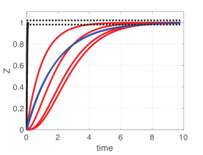
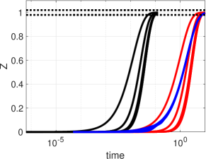
Figure 7: Cohesive versus rapid synchronization of response $Z$ with first-order agents. Step responses illustrating cohesion improvement during the transition with DSR. Blue: with DSR. Red: with nominal $K$ and $B$ without DSR. Solid black: with scaled dynamics $K$ and $B$ in Eq. (6) and without DSR. (left) Faster response leads to a reduction of cohesion deviation $\Delta$ as seen by comparing the case with scaled dynamics (solid black lines) and without scaled dynamics (red lines). (right) The normalized deviation $\Delta^{*}$ in Eq. (17) is not reduced substantially by increasing the response speed by scaling up the dynamics, i.e., through rapid synchronization, as seen when the time is represented in a log scale.

Nevertheless, rapid synchronization does not result in cohesion during the transition in terms of the normalized deviation $\Delta^{*}$ in Eq. (17). The responses remain substantially different from each other, as seen in Fig. 7. The normalized deviation $\Delta^{*}$ with rapid synchronization, achieved with a larger gain of $K_{gain}=77.9$, is $\Delta^{*}=0.496$, which is the same as the normalized deviation of $\Delta^{*}=0.496$ for the nominal case without DSR . Thus, scaling up with larger gain $K_{gain}$ leads to a faster response (rapid synchronization), but it does not lead to improvements in the normalized cohesion $\Delta^{*}$.

Moreover, the rapid synchronization, achieved by scaling up the dynamics, requires a substantial increase in input magnitudes as seen in Fig. 8. The maximum input $U$ required without DSR is $0.499$, with DSR is about twice at $1.064$, and with the scaled-up dynamics ($K_{gain}=77.9$) is $38.97$, which is $77.96$ times more that the nominal case without DSR. Thus, the use of DSR increases the normalized cohesion without the substantial increase in input when compared to the rapid synchronization achieved by scaling-up of the dynamics.

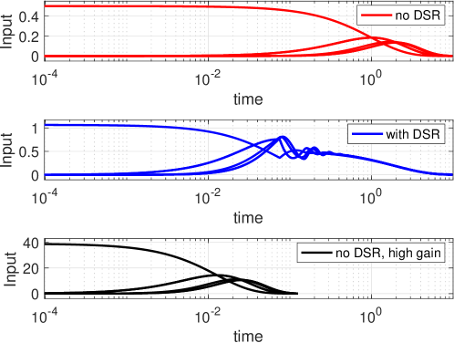
Figure 8: Input $U$ with first-order agents. Maximum input without DSR (top) is $0.499$, with DSR the maximum input (middle) is about twice at $1.064$, and with the scaled-up dynamics in Eq. (108) (bottom) is $38.97$, which is $77.9$ times more that the nominal case without DSR (top).

5.5 Example with higher-order dynamics

The impact of improved cohesion with DSR is illustrated in the following for agents with higher-order dynamics.

5.5.1 Higher-order dynamics example

Consider a second order dynamics ($r=2$) for the agents, using the same network as in Fig. 4, and therefore, the same pinned Laplacian $K$ and input matrix $B$ as in the first order example in Subsection (5.1). The system dynamics, with DSR, in Eq. (81) becomes

$$\ddot{Z}(t) =U(t)=-\beta K\left[2\alpha\dot{Z}(t)+\alpha^{2}Z(t)\right]$$ (109)

$$\quad\quad+\beta Bz_{s}^{*}(t)~{}+\left[I-\beta K\right]\hat{{Z}}^{(2)}(t,\tau).$$

The DSR term $\hat{Z}^{(2)}(t,\tau)$ is as in Eq. (80),

$$\hat{Z}^{(2)}(s,\tau) =\left[f(s)\frac{1-e^{-\tau s}}{\tau}\right]^{2}Z(s)={\mathcal{F}}(s)P(s),$$ (110)

with time domain representation, when the filter is selected as $f(s)=\frac{\Omega}{s+\Omega}$,

$$\frac{d}{dt}\hat{Z}^{(1)}(t,\tau) =-\Omega\hat{Z}^{(1)}(t,\tau)+\Omega\frac{Z(t)-Z(t-\tau)}{\tau}$$ (111)

$$\frac{d}{dt}\hat{Z}^{(2)}(t,\tau) =-\Omega\hat{Z}^{(2)}+\Omega\frac{\hat{Z}^{(1)}(t)-\hat{Z}^{(1)}(t-\tau)}{\tau}.$$

The DSR parameters are selected similar to the first-order case. The delay is selected as $\tau=0.075$ s and the parameter $\alpha=1.195$. With the DSR-parameter $\beta=2$, the lower bound ${\epsilon_{\lambda}}$ is selected as in Eq. (98), ${\epsilon_{\lambda}}={\overline{\epsilon_{\lambda}}}=1.14$. The expression for stability in Eq. (96) was verified numerically as in Remark 14, where the lhs of Eq. (96) was computed over the imaginary axis with the filter selected as a low pass filter as in Eq. (111) and $\Omega=\alpha/10$.

5.5.2 Results with higher-order dynamics

The use of DSR leads to more cohesive response when compared to the case without DSR. The response with DSR is shown in Fig. 9. It is compared to the case without DSR, i.e., $\hat{{Z}}^{(2)}(t,\tau)=0$ in Eq. (109) and a larger parameter $\alpha=1.69$ so that the maximum input without DSR of $2.82$ is similar to the maximum input with DSR of $2.8$, as shown in Fig. 10. The use of DSR results in similar settling time of $6$ s when compared to $5.3$ s without DSR. The cohesion deviation is reduced from $\Delta=1.04,~{}\Delta^{*}=.17$ without DSR to $\Delta=0.63,~{}\Delta^{*}=0.11$ with DSR. Thus, the simulations show that with similar-sized input, the DSR approach leads to increased cohesion for networked agents with higher-order dynamics.

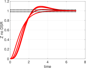
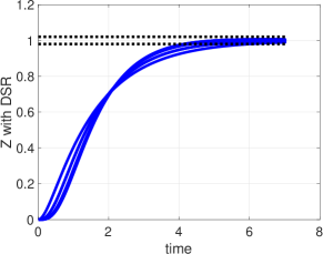
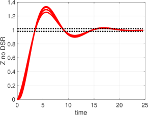
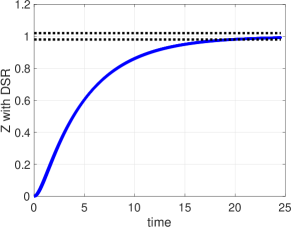
Figure 9: Step response $Z$ with second-order agents with real eigenvalues (top) and complex eigenvalues (bottom). (Top left) Without DSR, i.e., $\hat{{Z}}^{(2)}(t,\tau)=0$ and $\alpha=1.69$ in Eq. (109). (Top right) More cohesive response with DSR as in Eq. (109). (Bottom left) Without DSR, i.e., $\hat{{Z}}^{(2)}(t,\tau)=0$ and $\alpha=1.69$ in Eq. (109). (Bottom right) More cohesive response with DSR as in Eq. (109).

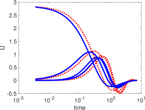
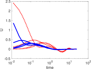
Figure 10: Input $U$ with second-order agents. (Left) real-eigenvalue case. Maximum input without DSR (red, dotted line) is $2.82$, which is similar to the case with DSR (blue, solid line) with a maximum input of $2.8$. (Right) complex-eigenvalue case. Maximum input without DSR (red, dotted line) is $2.41$, and with DSR (blue, solid line) with a maximum input of $1.36$.

5.5.3 Results with complex eigenvalues

Additional simulations were performed for higher-order dynamics (see Figs. 9, 10) for the complex-eigenvalue case. This was achieved by adding edges from nodes $4,5,6$ to node $1$ in Fig. 4. This leads to a loss of topological ordering, and leads to complex eigenvalues for the pinned Laplacian $K$. The resulting response tends to be more oscillatory.

Nevertheless, reductions are seen in the cohesion deviation, as with the case for higher-order dynamics with real-valued eigenvalues. With the DSR-parameters $\tau=0.075$ s, $\beta=20$, and $\alpha=1.195$, the expression for stability in Eq. (96) was verified numerically as in Remark 14. The use of DSR results in similar settling time of $19.9$ s when compared to $18.5$ s without DSR. The cohesion is improved from $\Delta=1.17,\Delta^{*}=0.058$ without DSR to $\Delta=0.176,\Delta^{*}=0.009$ with DSR. Thus, the simulations show that with similar settling time, the DSR approach leads to increased cohesion for networked agents with higher-order complex dynamics.

The MATLAB code is attached as an Appendix.

5.6 Limitations and future work

Overall, the simulation results show substantial cohesion improvement with the DSR approach, even for agents with higher-order dynamics. In general, network properties such as synchronization can be maintained if the network is jointly connected (instead of being always connected). Additional work is needed to extend the current work to develop conditions for cohesion improvements with the DSR approach for such time-varying networks. Similarly, there is potential to extend the DSR approach to improve cohesion during finite-time and fixed-time synchronization.

6 Conclusions

This work proposed a new delayed-self reinforcement (DSR) approach that enables cohesive response of multi-agent networks, during transitions from one cohesive operating point to another. Stability conditions were developed for the delay-based implementation of the proposed control law for general directed-graph networks. The potential for substantial improvements with the proposed DSR approach was illustrated with a simulation example and comparative analysis with and without DSR. The main advantage of the DSR approach is that it does not require reorganization of the network or increases in the response speed of the network to improve cohesion. Moreover, the method is applicable to agents with higher-order heterogeneous dynamics.

7 Acknowledgment

This work was partially supported by NSF grant CMII 1536306.

Appendix

⬇

1% Simulations for problem in Automatica Paper

2% Second order Complex Case system

3% March 14 2020

4

5 clear all

6 nfig=0;

7

8%%%%%%%%%%%%%%%%%%%%%%%%%%%%%%%%%%%%%%%%%%%%%%%%%%%%%%%%%%%%%%%%%

9 %%%% Step 1: stimulate step response of the system without DSR

10%%%%%%%%%%%%%%%%%%%%%%%%%%%%%%%%%%%%%%%%%%%%%%%%%%%%%%%%%%%%%%%%%

11

12 N=6; nleader=1;

13 K = zeros(N,N); % initialize the K matrix

14 B = zeros(N,1); % initialize the B matrix

15 K(1,1:6) = [3 0 0 -1 -1 -1];

16 K(2,1:3) = [-1 2 -1];

17 K(3,1:3) = [-1 -1 2];

18 K(4,2:4) = [-1 0 1];

19 K(5,3:5) = [-1 0 1];

20 K(6,2:6) = [-1 -1 -1 -1 4];

21 % Pinning the leader

22 K(nleader,nleader) = K(nleader,nleader)+1;

23 B(nleader) = 1;

24

25 % Need to choose beta to satisfy: \beta > \frac{1}{\rho_{i} \cos{\phi_i} },

26 % say 2 times the maximum of rhs over all i

27 lambda = eig(K); % the eigenvalues of K

28 Ts = 7.5;

29 tau = Ts/100;

30

31 % similar settling time but for a second order system

32 alpha_no_dsr = 1.69

33 beta =20

34 alpha =alpha_no_dsr/sqrt(beta)

35

36 alpha_hat1 = 2*alpha; alpha_hat0 = alpha*alpha;

37 alpha_hat1_nodsr = 2*alpha_no_dsr;

38 alpha_hat0_nodsr = alpha_no_dsr*alpha_no_dsr;

39

40%%%%%%%%%%%%%%%%%%%%%%%%%%%%%%%%%%%%%%%%%%%%%%%%%%%%%%%%%%%%%%%%%

41 %%%% Step 2: simulate the system without the delayed control scheme Second Order System

42%%%%%%%%%%%%%%%%%%%%%%%%%%%%%%%%%%%%%%%%%%%%%%%%%%%%%%%%%%%%%%%%%

43

44 % simulate the system without the delayed control scheme

45 zK = zeros(size(K)); iK = eye(size(K)); % zero and identity matrices

46 % define the system

47

48 Aa = [zK iK; -alpha_hat0_nodsr*K -alpha_hat1_nodsr*K];

49 Ba = [0*B; alpha_hat0_nodsr*B]; Ca = zeros(1,2*N); Ca(1,N)=1; Da = [];

50 Cvel = zeros(1,2*N); Cvel(1,N)=1;

51 Sysnodelay = ss(Aa, Ba, Ca, Da);

52 eigA = eig(Aa);

53

54 vd= 1; % final desired state

55 percentval_ts=2; % how to define final value

56 noiselevel = 0;

57

58 % Find the setting time and redo with specify time vector

59 [Y,t,X] = step(Sysnodelay);

60 tsteps = 2000; % time steps in the simulations

61 tmax = max(t); t=1:1:tsteps; t = t*tmax/tsteps;

62 [Y,t,X] = step(Sysnodelay,t);

63 X_no_dsr = X(:,1:N);

64 V_no_dsr = X(:,N+1:2*N);

65 U_no_dsr = -alpha_hat0_nodsr*K*X_no_dsr’ -alpha_hat1_nodsr*K*V_no_dsr’ +alpha_hat0_nodsr*B;

66

67%%%%%%%%%%%%%%%%%%%%%%%%%%%%%%%%%%%%%%%%%%%%%%%%%%%%%%%%%%%%%%%%%

68%%%% Step 3: Stability of system with DSR

69%%%%%%%%%%%%%%%%%%%%%%%%%%%%%%%%%%%%%%%%%%%%%%%%%%%%%%%%%%%%%%%%%

70

71 eigK = eig(K);

72 eps_lamdba = min(abs(beta*eigK./(1-beta*eigK)))

73 %%% check for stability

74 Omega = .1*alpha; % filter selection

75 w =1:Omega/10:100*Omega;

76 fs = Omega./abs((j*w) + Omega) ;

77 lhs = (1-exp(-tau*j*w)).*fs;

78 lhs = max(abs(lhs));

79 rhs = tau*(eps_lamdba.^(1/2))*alpha;

80 if rhs >= lhs

81 lhs_rhs = [ lhs rhs]

82 disp(’stability condition is met’)

83 else

84 lhs_rhs = [ lhs rhs]

85 disp(’Problem: stability condition is not met’)

86 return

87 end

88

89

90%%%%%%%%%%%%%%%%%%%%%%%%%%%%%%%%%%%%%%%%%%%%%%%%%%%%%%%%%%%%%%%%%

91%%%% Step 4: simulate the system with DSR

92%%%%%%%%%%%%%%%%%%%%%%%%%%%%%%%%%%%%%%%%%%%%%%%%%%%%%%%%%%%%%%%%%

93

94 Aadsr = [zK iK; -alpha_hat0*K -alpha_hat1*K];

95 Badsr = [0*B; alpha_hat0*B]; Ca = zeros(1,2*N); Ca(1,N)=1; Da = [];

96

97 Nsim = N*4; dsr_or_not=1;

98 history = [zeros(Nsim,1)];

99 Param_dde = [alpha tau beta N Omega dsr_or_not];

100 %sol = dde23(ddefun,lags,history,tspan,options)

101 sol = dde23(@ddefun,[tau],history,[0, tmax],[],Aadsr,Badsr,K,Param_dde);

102 y_dsr = deval(sol,t);

103 % Definitions in dde23 function dydt = ddefun(t,y,ydel,Aa,Ba,K,Param)

104 %alpha = Param(1); tau = Param(2); beta = Param(3);

105 %N = Param(4); Omega = Param(5); dsr_or_not = Param(6);

106

107

108 X_dsr = y_dsr(1:N,:);

109 V_dsr = y_dsr(N+1:2*N,:);

110 Phat2_dsr = y_dsr(3*N+1:4*N,:);

111 U_dsr = -beta*alpha_hat0*K*X_dsr -beta*alpha_hat1*K*V_dsr +beta*alpha_hat0*B + (eye(size(K))-beta*K)*Phat2_dsr;

112

113

114 nfig=nfig+1; figure(nfig)

115 plot(t,X_no_dsr,’r:’,t,X_dsr,’b’,’LineWidth’,4);

116 xlabel(’time’); ylabel(’Z’);

117 set(gca,’FontSize’,20)

118 pause(0.01)

119 % Blue(DSR) Red(no-DSR)

120 %legend(’no DSR’,’with DSR’)

121

122 nfig=nfig+1; figure(nfig)

123 semilogx(t,U_no_dsr,’r:’,t,U_dsr,’b’, ’LineWidth’,4);

124 xlabel(’time’); ylabel(’U’);

125 set(gca,’FontSize’,20)

126 pause(0.01)

127 %Blue(DSR) Red(no-DSR)

128 saveas(gcf,’fig_hdf_U_comparison_rev_resp’,’epsc’)

129

130 Max_input_U_dsr = max(max(U_dsr))

131 Max_input_U_no_dsr = max(max(U_no_dsr))

132

133 return

134

135%%%%%%%%%%%%%%%%%%%%%%%%%%%%%%%%%%%%%%%%%%%%%%%%%%%%%%%%%%%%%%%%%

136% function to define the derivative for DDE solution

137%%%%%%%%%%%%%%%%%%%%%%%%%%%%%%%%%%%%%%%%%%%%%%%%%%%%%%%%%%%%%%%%%

138

139function dydt = ddefun(t,y,ydel,Aa,Ba,K,Param)

140% Differential equation function

141alpha = Param(1); tau = Param(2); beta = Param(3);

142N = Param(4); Omega = Param(5); dsr_or_not = Param(6);

143

144% define current and delayed states X=[P;Pdot], Phat1, Phat2

145yd =1;

146X = y(1:N*2,1);

147

148P = y(1:N,1);

149Pdel = ydel(1:N,1);

150Phat1 = y((N*2 +1):N*3,1);

151Phat1del = ydel((N*2 +1):N*3,1);

152Phat2 = y((N*3 +1):N*4,1);

153Phat2del = ydel((N*3 +1):N*4,1);

154

155dot_Phat1 = -Omega*Phat1 +Omega*(P -Pdel)/tau;

156dot_Phat2 = -Omega*Phat2 +Omega*(Phat1 -Phat1del)/tau;

157dot_X = [eye(N,N) zeros(N,N); zeros(N,N) beta*eye(N,N)]*Aa*X +beta*Ba*yd + dsr_or_not*[zeros(N,1); (eye(size(K))-beta*K)*Phat2];

158

159dydt = [dot_X ; dot_Phat1; dot_Phat2];

160end % ddex4de

References

- [1] Wei Ren. Multi-vehicle consensus with a time-varying reference state. Systems and Control Letters, 56:474–483, July 2007.
- [2] Alireza Talebpour and Hani S. Mahmassani. Influence of connected and autonomous vehicles on traffic flow stability and throughput. Transportation Research Part C: Emerging Technologies, 71:143 – 163, 2016.
- [3] A Huth and C Wissel. The simulation of the movement of fish schools. Journal of Theoretical Biology, 156(3):365–385, Jun 7 1992.
- [4] Tamás Vicsek, András Czirók, Eshel Ben-Jacob, Inon Cohen, and Ofer Shochet. Novel type of phase transition in a system of self-driven particles. Phys. Rev. Lett., 75:1226–1229, Aug 1995.
- [5] A. Attanasi, A. Cavagna, L Del Castello, I. Giardina, T.S. Grigera, A. Jelic, S. Melillo, L. Parisi, O. Pohl, E. Shen, and M. Viale. Information transfer and behavioural inertia in starling flocks. Nature Physics, 10(9):615–698, Sep 1 2014.
- [6] A. Jadbabaie, Jie Lin, and A. S. Morse. Coordination of groups of mobile autonomous agents using nearest neighbor rules. IEEE Transactions on Automatic Control, 48(6):988–1001, June 2003.
- [7] Wei Ren and R. W. Beard. Consensus seeking in multiagent systems under dynamically changing interaction topologies. IEEE Transactions on Automatic Control, 50(5):655–661, May 2005.
- [8] R. Olfati-Saber. Flocking for multi-agent dynamic systems: algorithms and theory. IEEE Transactions on Automatic Control, 51(3):401–420, March 2006.
- [9] Hanlei Wang. Consensus of networked mechanical systems with communication delays: A unified framework. IEEE Transactions on Automatic Control, 59:1571–1576, Jun. 2014.
- [10] Jiakang Zhou and Qinglei Huand Michael I. Friswell. Decentralized finite time attitude synchronization control of satellite formation flying. Journal of Guidance, Control, and Dynamics, 36:185–195, Jan. 2013.
- [11] Yan-Wu Wang, Xiao-Kang Liu, Jiang-Wen Xiao, and Yanjun Shen. Output formation-containment of interacted heterogeneous linear systems by distributed hybrid active control. Automatica, 93:26–32, July 2018.
- [12] Jorge Cortés. Finite-time convergent gradient flows with applications to network consensus. Automatica, 42(11):1993 – 2000, 2006.
- [13] J. Bu, M. Fazel, and M. Mesbahi. Accelerated consensus with linear rate of convergence. In 2018 Annual American Control Conference (ACC), pages 4931–4936, June 2018.
- [14] Shihua Li, Haibo Du, and Xiangze Lin. Finite-time consensus algorithm for multi-agent systems with double-integrator dynamics. Automatica, 47(8):1706 – 1712, 2011.
- [15] Bin Hu, Zhi-Hong Guan, and Minyue Fu. Distributed event-driven control for finite-time consensus. Automatica, 103:88 – 95, 2019.
- [16] Stephen Boyd, Persi Diaconis, and Lin Xiao. Fastest mixing markov chain on a graph. SIAM Rev., 46(4):667–689, April 2004.
- [17] Ruggero Carli, Fabio Fagnani, Alberto Speranzon, and Sandro Zampieri. Communication constraints in the average consensus problem. Automatica, 44(3):671–684, Mar 2008.
- [18] Shize Su and Zongli Lin. Connectivity enhancing coordinated tracking control of multi-agent systems with a state-dependent jointly-connected dynamic interaction topology. Automatica, 101:431–438, March 2019.
- [19] D. E. Rumelhart, G. E. Hinton, and R. J. Williams. Learning Internal Representations by Error Propagation, pp. 318-362, in D. E. Rumelhart and J. L. McClelland (eds.) Parallel Distributed Processing, Vol. 1 . MIT Press, Cambridge, MA, 1986.
- [20] Ning Qian. On the momentum term in gradient descent learning algorithms. Neural Networks, 12(1):145 – 151, 1999.
- [21] S. Devasia. Rapid Information Transfer in Swarms under Update-Rate-Bounds using Delayed Self-Reinforcement. ASME Journal of Dynamic Systems Measurement and Control, 141(8):#081009 1–9, August Aug, 2019.
- [22] W. L. Miranker. Existence, Uniqueness and Stability of Solutions of Systems of Nonlinear Difference-Differential Equations. Journal of Mathematics and Mechanics, 11(1):101–107, 1962.
- [23] Richard Bellman and Kenneth L. Cooke. Differential-Difference Equations, Vol 6, Series of Monographs and Textbooks, Mathematics in Science and Engineering. Academic Press, New York, 1963.
- [24] R. M. Corless, G. H. Gonnet, D. E. G. Hare, D. J. Jeffrey, and D. E. Knuth. On the lambertw function. Advances in Computational Mathematics, 5(1):329–359, Dec 1996.
- [25] F. M. Asl and A. G. Ulsoy. Analysis of a system of linear delay differential equations. Journal of Dynamic Systems Measurement and Control -Transactions of the ASME, 125(2):215–223, JUN 2003.
- [26] Sun Yi, Patrick W Nelson, and A. Galip Ulsoy. Time-Delay Systems Analysis and Control Using the Lambert W Function. World Scientific - Technology & Engineering, Hackensack, NJ, 2010.
- [27] A. G. Ulsoy. Time-Delayed Control of SISO Systems for Improved Stability Margins. Journal of Dynamic Systems Measurement and Control -Transactions of the ASME, 137(5):041014–041014–12, Apr 2015.
- [28] Jie Chen. On computing the maximal delay intervals for stability of linear delay systems. IEEE Transactions on Automatic Control, 40(6):1087–1093, Jun 1995.
- [29] N. Olgac and R. Sipahi. An exact method for the stability analysis of time-delayed linear time-invariant (lti) systems. IEEE Transactions on Automatic Control, 47(5):793–797, May 2002.
- [30] N Olgac and R Sipahi. The cluster treatment of characteristic roots and the neutral type time-delayed systems. Journal of Dynamic Systems Measurement and Control , 127(1):88–97, MAR 2005.
- [31] W. Qiao and R. Sipahi. Consensus control under communication delay in a three-robot system: Design and experiments. IEEE Transactions on Control Systems Technology, 24(2):687–694, March 2016.
- [32] R. K. Brayton and R. A. Willoughby. On the numerical integration of a symmetric system of difference-differential equations of neutral type. Journal of Mathematical Analysis and Applications, 18 (1):182–189, April 1967.
- [33] N. D. Hayes. Roots of the transcendental equation associated with a certain difference-differential equation. Journal of the London Mathematical Society, s1-25(3):226–232, 1950.
- [34] R. Olfati-Saber, J.A. Fax, and R.M. Murray. Consensus and cooperation in networked multi-agent systems. Proceedings of the IEEE, 95(1):215–233, Jan 2007.
- [35] W. T. Tuttle. Graph Theory. Cambridge University Press, Cambridge, 2001.
- [36] Y. E. Nesterov. A Method of Solving a Convex Programming Problem with Convergence Rate of . Soviet Mathematics Doklady, 27(3):372–376, 1983.
- [37] S. Devasia. Faster Response in Bounded-Update-Rate, Discrete-time Networks using Delayed Self-Reinforcement. International Journal of Control, Accepted, 2019, DOI: 10.1080/00207179.2019.1644537.
- [38] Yongcan Cao and Wei Ren. Multi-Agent Consensus Using Both Current and Outdated States with Fixed and Undirected Interaction. Journal of Intelligent & Robotic Systems, 58(1):95–106, April 2010.
- [39] Hossein Moradian and Solmaz Kia. Accelerated average consensus algorithm using outdated feedback. In 2019 European Control Conference ECC, June 25-28, Napoli, Italy, 2019.
- [40] S. Devasia. Accelerated Consensus for Multi-Agent Networks through Delayed Self Reinforcement. Proceedings of the IEEE International Conference on Industrial Cyber-Physical Systems, Taipei, Taiwan, May 6-9, May, 2019.
- [41] J.M. Ortega. Matrix Theory, Classics in applied mathematics; vol. 3). Plenum Press, New York, 1987.
- [42] Yutaka Yamamoto. Equivalence of internal and external stability for a class of distributed systems. Mathematics of Control, Signals and Systems, 4(4):391–409, December 1991.
- [43] A. Isidori. Nonlinear Control Systems: An Introduction. Springler-Verlag, 1989.