Electrostatic quantum dot confinement in phosphorene

Abstract

We consider states localized by electrostatic potentials in phosphorene using atomistic tight-binding approach. From the tight-binding spectra of states confined in parabolic potential we extract effective masses for conduction band electrons moving along the armchair and zigzag crystal directions by a fit to the harmonic oscillator spectrum. The masses derived in this way are used for a simple single-band effective-mass model which, as we find, reproduces very well the tight-binding energy spectra in external magnetic field, the confined probability densities, and the interaction effects. We study the confined states in the conduction band and find that both methods already for small quantum dots produce Wigner crystallization with separated single-electron islands. The effective-mass model works with a slightly worse precision for confined states of the valence band. The continuum approach deviates considerably from the tight-binding model only in the limit of extremely strong lateral confinement.

I introduction

Black phosphorus (BP) is a layered semiconductor material that attracts a growing attention for its basic properties and possible applications aniso ; 14 ; otpo ; rev ; fukuoka15 . BP with direct band gap anisobp that falls within the visible range for few-layer systems prbgap ; thbgnl ; fofo is investigated for optoelectronic applications otpo . Separation of few-layer material down to a monolayer (phoshorene) fosf14 is now routinely accomplished. The lateral confinement for optics is achieved in nanocrystal Lee17 ; Sun15 ; Wang18 ; BPQD18 ; Saroka ; s2 ; s3 ; pet1 quantum dots (QDs) that support confinement of both electrons and holes with by a mere finite size of the medium.

Gating of BP grown on nonmetallic substrates allows for fabrication of field effect transistors Bfet14 that recently reached a long-term air stability at room temperature he19 ; bl19 . The integer hhe ; ehe and fractional quantum Hall qhe effects, the latter being a fingerprint of strong correlations between interacting carriers, has already been reported qhe . The electrostatic QDs in bulk semiconductors eqd , bilayer graphene prx or carbon nanotubes laird with their clean confinement independent of the nanocrystal edges, allow for precise studies of localized states, energy spectra, coherence times eqd , electron-electron interactions reim as well as for control of the charge ceqd1 ; ceqd2 and spin eqds degrees of freedom. Although the advanced stage of BP field effect transistors has been reached ehe ; Bfet14 ; he19 ; bl19 ; hhe ; qhe so far there are neither experimental nor theoretical literature on electrostatic QD confinement in BP.

In this paper we study a single electron and an electron pair confined in a phosphorene QD by an external potential that can be induced by electrostatic confinement. The electrostatic confinement potential is usually parabolic near its minimum lis . For materials with a parabolic dispersion relation the quantum harmonic oscillator is formed in this way, with the Fock-Darwin dependence on the external magnetic field for the isotropic case reim . The anisotropy of phoshorene crystal structure rev is translated to the in-plane anisotropy of the valence and conduction bands aniso ; anisobp ; 18 ; tibikast1 ; tibikast2 , with the effective masses along the zigzag direction that are much larger than in the armchair direction 18 . The electrostatic BP quantum dots are promising for observation of strong interaction effects due to large effective masses in one of the directions and for tuning the interaction by orientation of the confinement potential anisotropy, and not the size of the dot, as for materials with isotropic effective masses. The BP energy bands deviate from parabolic prbli19 ; kdotp2 ; kdotp1 near the conduction and valence band extrema. Due to the non-parabolicity a precise continuum description calls for $k\cdot p$ modelling of the low energy bands with the coupling between the conduction and valence bands kdotp2 ; kdotp3 ; kdotp4 ; kdotp5 . The coupling is relatively weak for monolayer BP due to the large band gap prbgap ; fofo . In phosphorene the Landau levels are nearly linear on the external magnetic field and the non-linear corrections turn out to be small kdotp6 ; small . On the other hand already for bilayer phosphorene the energy spectra in external magnetic field are very complex, non-linear and corresponding to different effective masses for each level kdotp6 . The relatively simple form of Landau levels for phosphorene kdotp6 ; small motivated us to look for description of the confined states in a parabolic single-band effective mass modeling. We extract the effective masses from the tight-binding model by imposing a parabolic confinement potential. Next we use the effective masses as external potential parameters for which the tight-binding calculations approximate best the quantum harmonic osillator spectrum for $B=0$ with its characteristic degeneracies and energy spacings. Although the tight-binding spectrum deviates from the exact quantum harmonic oscillator, the single and two-electron levels calculated by the tight-binding method can be surprisingly well reproduced by the simple single-band effective-mass model.

II Theory

II.1 single-electron Hamiltonian

We consider a monolayer BP (see Fig. 1) with zigzag lines extended along the $y$ direction and the armchair lines along the $x$ axis. We use the effective tight-binding Hamiltonian of Ref. tibikast1 ,

$$H_{TB}=\sum_{kl}t_{kl}p_{kl}c_{k}^{\dagger}c_{l}+\sum_{k}V_{k}c^{\dagger}_{k}c_{k}+\frac{g\mu_{B}B}{2}\sigma_{z},$$ (1)

where the first sum describes the hopping between the neighbor atoms, and $p_{kl}$ is the Peierls phase that introduces the orbital effects of the magnetic field $p_{kl}=e^{i\frac{e}{\hbar}\int_{\vec{r_{k}}}^{\vec{r_{l}}}\vec{A}\cdot\vec{dl}}$ to the hopping elements. We use the symmetric gauge ${\bf A}=(A_{x},A_{y},A_{z})=(-By/2,Bx/2,0)$ for the perpendicular magnetic field $(0,0,B)$ The hopping integrals $t_{kl}$ adopted from Ref. tibikast1 are listed in Table 1. The pairs of ions that correspond to the two largest absolute values of $t_{kl}$ are linked in Fig. 1 by blue ($t_{kl}=-1.22$ eV) and red ($t_{kl}=3.665$ eV) lines. The second sum of Eq. (1) introduces the external potential, and the last term stands for the Zeeman effect with the Landé factor $g=2$, and Bohr magneton $\mu_{B}$. We consider a finite rectangular flake of phosphorene with a side length of 87 nm in the $x$ direction and 44 nm in the $y$ direction with over 100 thousand ions. The size of the flake is larger than the confinement area of low-energy states considered below.

For the external potential we use the harmonic oscillator potential

$$V(x,y)=\frac{1}{2}m_{x}\omega^{2}x^{2}+\frac{1}{2}m_{y}\omega^{2}y^{2},$$ (2)

where $\hbar\omega$ is the oscillator energy, the $m_{x}$ and $m_{y}$ are fit parameters for the electron effective masses in the armchair and zigzag directions, respectively. For $m_{x}\neq m_{y}$ potential (2) is anisotropic. In Eq. (1) $V_{k}$ is the potential on $k$th ion, $V_{k}=V(x_{k},y_{k})$, where $x_{k}$, and $y_{k}$ are the coordinates of the $k$th ion. We establish $m_{x}$ and $m_{y}$ in the potential of Eq. (2) as fit parameters for the tight-binding spectrum to reproduce the harmonic oscillator spectrum at $B=0$.

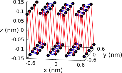
Figure 1: Crystal structure of phosphorene with zigzag lines extended along the $y$ direction. The zigzag bonds appear on two parallel planes shifted in the $z$ direction. The links between the atoms show the pairs of the largest absolute values of the hopping energy (see Table I). The nearest neighbors within the zigzag chain are linked with the blue lines that are spaced by 2.22 Å  with the hopping energy of $-1.22$ eV. The red lines show the nearest-neighbor links between the zigzag chains of separate planes that are 2.24 Å  long with the hopping energy of $3.665$ eV.

II.2 confined electron pair in the tight-binding approach

We calculate the spectrum for a confined electron pair using the Hamiltonian,

$${H}_{2e}=\sum_{i}{d}^{\dagger}_{i}{d}_{i}E_{i}+\frac{1}{2}\sum_{ijkl}{d}^{\dagger}_{i}{d}^{\dagger}_{j}{d}_{k}{d}_{l}V_{ijkl},$$ (3)

where ${d}^{\dagger}_{i}$ is the electron creation operator for the single-electron energy level $E_{i}$ and the Coulomb matrix elements read

$$V_{ijkl}=\kappa\langle{\psi_{i}(\mathbf{r_{1}})\psi_{j}(\mathbf{r_{2}})\frac{1}{|\mathbf{r_{12}}|}}{\psi_{k}(\mathbf{r_{1}})\psi_{l}(\mathbf{r_{2}})}\rangle,$$ (4)

where $\kappa=e^{2}/(4\pi\epsilon\epsilon_{0})$, and $\psi$’s standing for eigenstates of single-electron Hamiltonian (1). We consider that the phoshorene is embedded in Al₂O₃ matrix and use its dielectric constant $\epsilon_{0}=9.1$. We integrate the Coulomb elements for the single-electron wave functions $\psi$ spanned by the atomic orbitals $3p_{z}$ of $P$ atoms,

$$\psi_{i}({\bf r}_{i})=\sum_{k}C^{i}_{k}p_{z}^{k}({\bf r}_{1}),$$ (5)

$$V_{ijkl} = \kappa\langle\psi_{i}({\bf r_{1}})\psi_{j}({\bf r_{2}})|\frac{1}{|{r_{12}}|}|\psi_{k}({\bf r_{1}})\psi_{l}({\bf r_{2}})\rangle$$ (6)

$$= \kappa\sum_{\begin{subarray}{c}a,\sigma_{a};b,\sigma_{b};\\ c,\sigma_{c};d,\sigma_{d}\end{subarray}}C_{a,\sigma_{a}}^{i*}C_{b,\sigma_{b}}^{j*}C_{c,\sigma_{c}}^{k}C_{d,\sigma_{d}}^{l}\delta_{\sigma_{a};\sigma_{d}}\delta_{\sigma_{b};\sigma_{c}}\times$$

$$\langle p_{z}^{a}({\bf r}_{1})p_{z}^{b}({\bf r_{2}})|\frac{1}{|{r_{12}}|}|p_{z}^{c}({\bf r_{1}})p_{z}^{d}({\bf r_{2}})\rangle.$$

For the Coulomb integral we apply the two-center approximation c2 $\langle p_{z}^{a}({\bf r}_{1})p_{z}^{b}({\bf r_{2}})|\frac{1}{|{r_{12}}|}|p_{z}^{c}({\bf r_{1}})p_{z}^{d}({\bf r_{2}})\rangle=\frac{1}{r_{ab}}\delta_{ac}\delta_{bd}$ for $a\neq b$. The on-site integral ($a=b$) is calculated with $3p_{z}$ atomic orbitals, $p_{z}({\bf r})=Nz\left(1-\frac{Zr}{6}\right)\exp(-Zr/3)$, where $N$ is the normalization constant and $Z$ is the effective screened P nucleus charge as seen by $3p_{z}$ electrons. The single-center integral can then be calculated analytically, $I_{a=b}=\frac{3577}{46080}Z$ in atomic units. The Slater screening rules for $3p$ electrons in P atoms produce $Z=4.8$, then $I_{a=b}=10.14$ eV.

The Hamiltonian (3) is diagonalized with the configuration interaction approach in the basis of up to $\sim 1000$ two-electron Slater determinants constructed from the lowest-energy conduction-band eigenfunctions of the single-electron Hamiltonian (1).

$r_{kl}($Å$)$	$2.22$	$2.24$	$3.34$	$3.47$	$4.23$
$t_{kl}($eV$)$	-1.22	3.665	-0.205	-0.105	-0.055

Table 1: Hopping parameters for the effective tight-binding model of Ref. tibikast1 . The value of the hopping parameter $t_{ij}$ is given below the distance between P ions $r_{ij}$.

II.3 single-band effective-mass Hamiltonian

For description of the system in the effective-mass Hamiltonian we take the single-band approximation with the Hamiltonian,

$$H_{em} = \frac{\left(-i\hbar\frac{\partial}{\partial x}+e{A_{x}}\right)^{2}}{2m_{x}}+\frac{\left(-i\hbar\frac{\partial}{\partial y}+e{A_{y}}\right)^{2}}{2m_{y}}$$ (7)

$$+ V(x,y)+\frac{g\mu_{B}B}{2}\sigma_{z}.$$

To diagonalize this Hamiltonian we employ the finite-difference method with gauge-invariant discretization of Ref. governale and Peierls phases that account for the orbital effects of the magnetic field. For the mesh spacing $\Delta x$ in both $x$ and $y$ directions finite difference Hamiltonian defined by its action on the wave function $\Psi_{\mu,\nu}=\Psi(x_{\mu},x_{\nu})=\Psi(\mu\Delta x,\nu\Delta x),$

$$H_{fd}\Psi_{\mu,\nu} \equiv \frac{\hbar^{2}}{2m_{x}\Delta x^{2}}\left(2\Psi_{\mu,\nu}-C_{y}\Psi_{\mu,\nu-1}-C_{y}^{*}\psi_{\mu,\nu+1}\right)$$ (8)

$$+ \frac{\hbar^{2}}{2m_{y}\Delta x^{2}}\left(2\Psi_{\mu,\nu}-C_{x}\Psi_{\mu-1,\nu}-C_{x}^{*}\psi_{\mu+1,\nu}\right)$$

$$+ V_{\mu,\nu}\Psi_{\mu,\nu},$$

with $C_{x}=\exp(-i\frac{e}{\hbar}\Delta xA_{x})$ and $C_{y}=\exp(-i\frac{e}{\hbar}\Delta xA_{y})$.

With the eigenstates of Hamiltonian (8) we calculated the two-electron spectrum in the manner discussed above for the tight-binding method. The only difference is the on-site integral which is evaluated numerically

$$I_{a=b} = \int_{-\Delta x/2}^{\Delta x/2}dx_{1}\int_{-\Delta x/2}^{\Delta x/2}dy_{1}\int_{-\Delta x/2}^{\Delta x/2}dx_{2}\int_{-\Delta x/2}^{\Delta x/2}dy_{2}$$ (9)

$$\frac{1}{\sqrt{(x_{1}-x_{2})^{2}+(y_{1}-y_{2})^{2}}}$$

with the Monte Carlo method. With the finite difference mesh we cover the same area as in the tight-binding approach and use $\Delta x=0.2$ nm.

III Results

III.1 confined electrons of the conduction band

III.1.1 TB spectrum fit for the effective masses

We determine the effective masses by a fit of the tight-binding spectrum obtained for Hamiltonian (1) to the harmonic oscillator spectrum with potential (2). Note, that the fit involves variation of the confinement potential of Eq.(2) as the masses are varied. At $B=0$ the harmonic oscilator the $n$th excited energy level is $n+1$ fold degenerate (spin excluded) with the energy $n\hbar\omega$ above the ground state. For the fit we took $\hbar\omega=10$ meV and considered 15 lowest energy levels obtained with the tight-binding approach, including the ground-state. We looked for a minimal sum of squares of the energy difference between electron energy levels obtained with the tight-binding approach and the corresponding quantum harmonic oscillator energy levels. The best fit was obtained for $m_{x}=0.17037m_{0}$ and $m_{y}=0.85327m_{0}$, with the conduction band effective masses that fall within the range of the values indicated in the literature, e.g., $m_{x}/m_{0}=0.148$ nano , 0.16 016 , 0.166 kdotp6 , 0.17 18 , 0.2 scre2 , and $m_{y}/m_{0}=0.846$ kdotp6 , 1.12 18 , 1.237 nano , 1.24 016 . In the literature also values as large as $m_{y}=6.89m_{0}$ are used scre2 . Values large as the latter are obtained for strained phosphorene layers ntstrain . The optimal spacings between the excited states and the ground states are given in Table 2. The degeneracy of the excited energy levels is only approximate for the best fit. In Table 2 the largest energy diffrence $|\Delta E|$ between the tight-binding harmonic oscillator levels are 0.033 meV, 0.034 meV, 0.041 meV, and 0.117 meV for $n=1,2,3$, and $4$, respectively.

$n\hbar\omega$	$\Delta E_{TB}$					$\sqrt{\sum_{i}(E^{ex}_{i}-E^{tb}_{i})^{2}}$
10	10.000	10.033				0.0330
20	20.000	20.001	20.034			0.0340
30	29.959	29.961	30.013	30.021		0.0617
40	39.883	39.893	39.980	39.996	40.022	0.1614

Table 2: The energy spacings from the ground state in meV for 14 excited states of the conduction band with the tight-binding method for confinement potential given by Eq. (2). The electron effective masses fitted to the harmonic oscillator spectrum $m_{x}=0.17037m_{0}$, $m_{y}=0.85327m_{0}$ for $\hbar\omega=10$ meV and $B=0$. In the subsequent rows we group the nearly degenerate energy levels that for the quantum harmonic oscillator should be placed exactly at the energy of $n\hbar\omega$ above the ground state for $n=1,2,3$ and 4. The last column shows the root of the square distance between the harmonic oscillator spectrum and the tight-binding result for given $n$ in milielectronovolts.

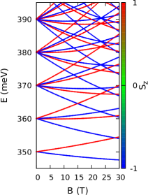
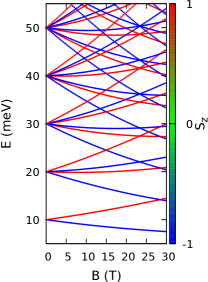
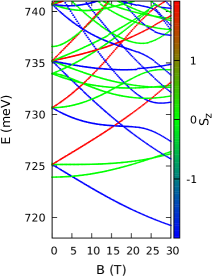
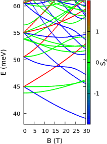
Figure 2: Tight-binding (a,b) spectrum and the results of the single-band effective-mass approximation (c,d) for a single (a,c) and two electrons (b,d) confined in potential (2) with $m_{x}=0.17037m_{0}$, $m_{y}=0.85327m_{0}$ and $\hbar\omega=10$ meV in the external magnetic field. The color of the line indicates the $z-$ component of the spin.

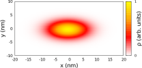
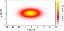
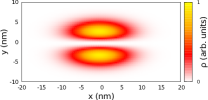
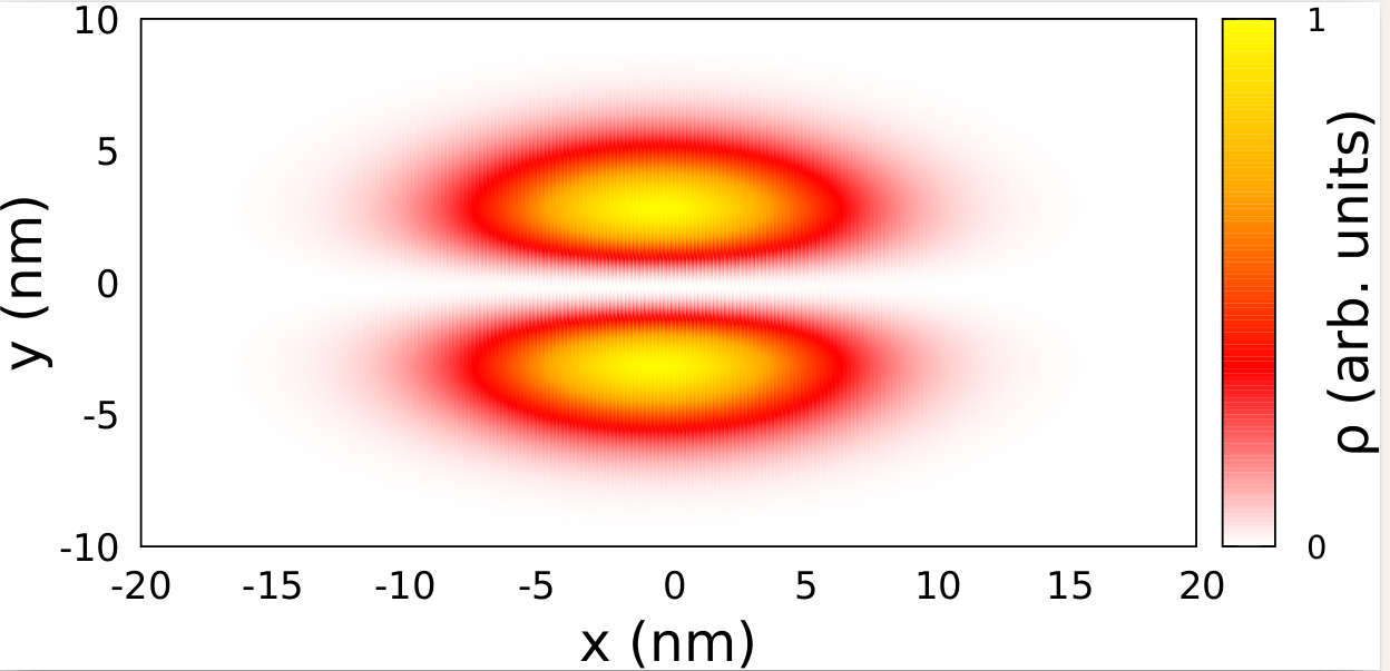
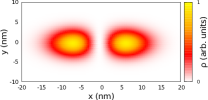
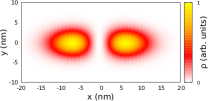
Figure 3: Probability density for the single-electron states calculated with the tight-binding – left column (a,c,e) and effective-mass approximation – right column (b,d,f). Panels (a,b) correspond to the single-electron ground state. Second (c,d) and third row (e,f) of plots correspond to the first and second excited single-electron states.

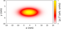
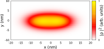
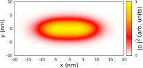
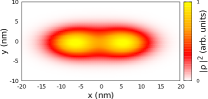
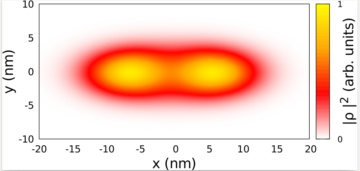
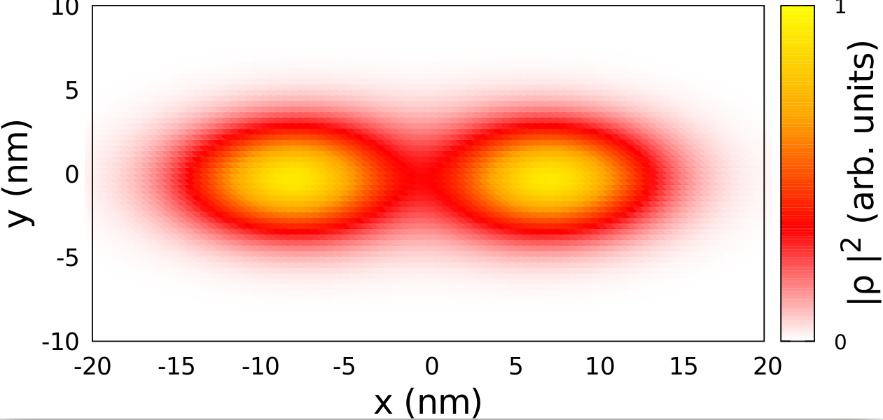
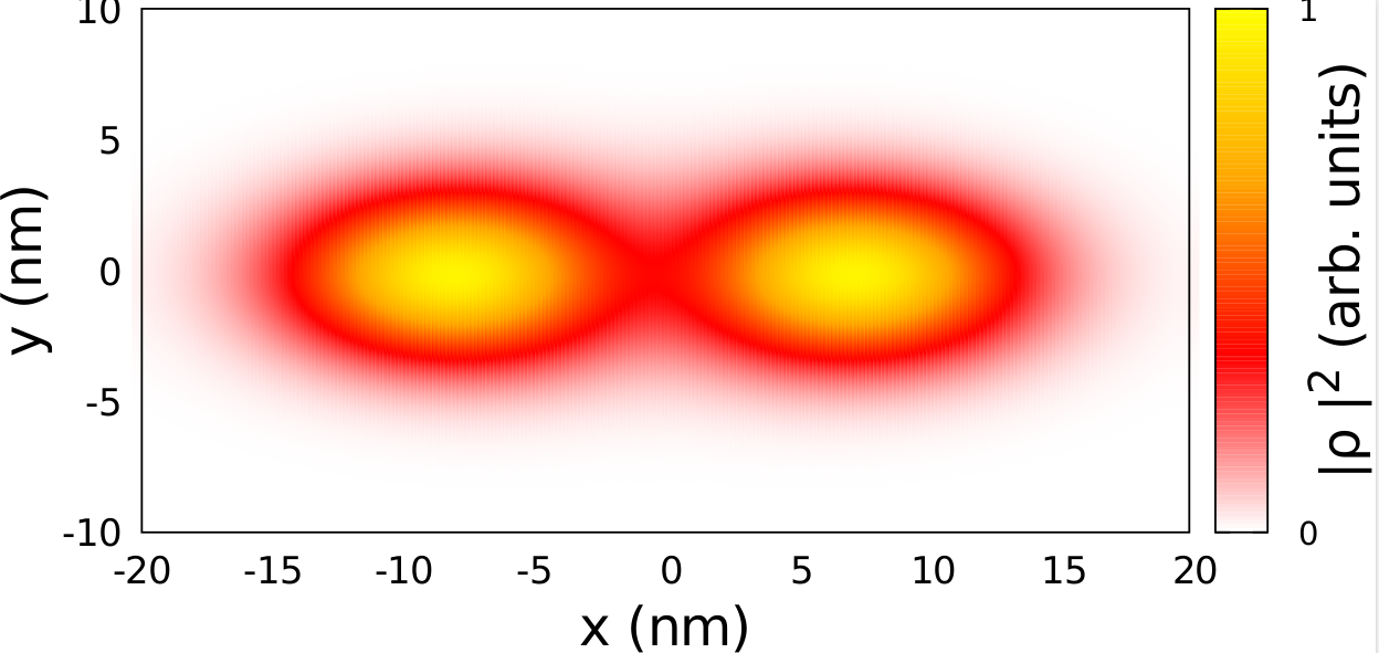
Figure 4: Probability density for two-electron ground-states calculated with the tight-binding – left column – (a,c,e,g,i) and effective-mass approximation –right column (b,d,f,h,j). Panels correspond to decreasing dielectric constant from top to bottom $\epsilon=\infty$ (a,b), $\epsilon=18.2$ (c,d), $\epsilon=9.1$ (e,f), and $\epsilon=4.55$ (g,h). In bulk of this work we apply $\epsilon=9.1$.

$n$	S/T	$\Delta E_{TB}$ (meV)	$\Delta E_{EM}$ (meV)
1	S	0	0
2	T	1.228	1.175
3	T	6.737	6.737
4	S	10.024	10.002
5	S	10.043	10.011
6	S	10.055	10.034
7	T	11.251	11.192
8	T	11.312	11.249
9	S	12.673	12.656
10	T	16.760	16.750

Table 3: The energy spacings in meV from the ground-state as calculated with the tight-binding method ($\Delta E_{TB}$) and with the effective-mass approximation ($\Delta E_{EM}$) for potential of Eq. 2 at $B=0$. The second column indicates the spin-singlet states by S and spin-triplet states by T.

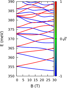
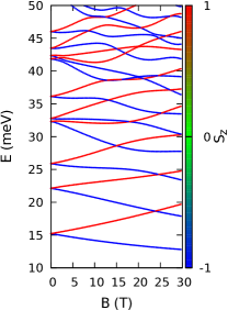
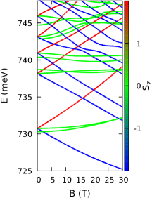
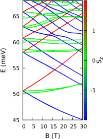
Figure 5: Same as Fig. 2 but for a Gaussian perturbation to the parabolic potential given by Eq. (10).

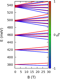
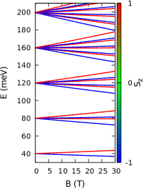
Figure 6: Tight-binding (a) and effective mass (b) single-electron spectrum for $\hbar\omega=40$ meV.

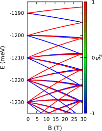
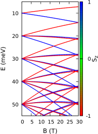
Figure 7: (a) The tight-binding energy spectrum for the valence-band confined states for inverted harmonic oscillator confinement with $\hbar\omega=10$ meV. (b) A single-particle spectrum in the effective-mass approximation (note the inverted scales for the energy and the spin). The results were obtained for hole effective masses obtained by a fit to the harmonic oscillator spectrum with $m_{x}=0.18972m_{0}$ and $m_{y}=1.15071m_{0}$.

III.1.2 Spectra in external magnetic-field and charge densities

The dependence of the single-electron energy levels in the external magnetic field is given in Fig. 2(a,c) with the same scale applied for the vertical and horizontal axes for the tight-binding [Fig. 2(a)] and continuum approach [Fig. 2(c)]. The probability density calculated with the tight-binding approach for the spin-down states: the ground state, the first and the second excited states are displayed in Fig. 3(a,c) and (e), respectively. For comparison the probability densities calculated with the effective-mass approximation are given in Fig. 3(b,d,f). The probability densities for these low-energy states are elongated along the armchair ($x$) direction and more strongly localized in the zigzag direction ($y$) and are very similar for the tight-binding Hamiltonian (left panels of Fig. 3) and in the single-band approximation (right panels of Fig. 3).

The energy spectra for the electron pair are plotted in Fig. 2(b,d). A more detailed comparison is given in Table 4 where the spacing from the ground state is given along with the information whether the state is spin-singlet or spin-triplet. The singlet-triplet order of the tight-binding energy levels is reproduced by the effective-mass approximation and the energy spacings as calculated by the continuum method agree with a precision of about 0.06 meV to the tight-binding results. In Fig. 4 we compare the results for the ground-state two-electron density as obtained with the tight-binding (left panels) and the continuum approach (right panels). Due to the large mass in the zigzag direction the ground states are localized near the $y=0$ line, to a quasi-one dimensional channel that promotes separation of single-electron charges. The panels from top to bottom of Fig. 4 correspond to decreasing dielectric constant. The results in Fig. 4(e,f) correspond to $\epsilon=9.1$ used in the bulk of this paper. As the screening of the interaction is reduced the charge density undergoes Wigner crystallization, with formation of the single-electron islands separated along the armchair direction ($x$ axis). Results of both the tight-binding and the effective-mass approaches are again very similar.

III.1.3 Non-parabolic confinement

In order to verify the effective-mass approximation for non-parabolic spectrum we introduced a perturbation to the potential given by Eq. (2) introducing a repulsive Gaussian centered at the $y$ axis, i.e. for potential

$$V_{p}(x,y)=V(x,y)+V_{z}\exp(-\frac{(y-y_{s})^{2}+x^{2}}{R^{2}}),$$ (10)

where $V(x,y)$ is given by Eq. (2), $V_{z}=30$ meV and $y_{s}=R=5$ nm. Comparison of the spectra is given in Fig. 5 for the single electron [Fig. 5(a,c)] and for the electron pair [Fig. 5(b,d)]. For the single-electron we notice that the perturbation that lowers the symmetry of the potential results in reduction of the degeneracy found for $B=0$. The energy levels enter into avoided crossings that replace the crossings of the high-symmetry case of Fig. 2(a,b). For the electron pair we find that the perturbation leads to a reduced triplet-singlet energy difference in the ground-state for $B=0$. The potential defect introduced above the potential minimum enhances the separation of the charges for the electron pair which Wigner localization in quasi one-dimensional systems results in the singlet-triplet degeneracy 1dszafran for fully separated single-electron islands. Overall agreement between the results of the effective-mass and tight-binding models is very good also for nonparabolic external potential.

III.1.4 Strong confinement

We find that the good quality of the effective-mass approximation holds for $\hbar\omega\leq 10$ meV. Deviations are found for extremely strong confinement. In the limit of strong confinement the effective-mass approximation can be expected fail since (i) the number of atoms in the confinement region becomes limited and (ii) the stronger confinement induces larger contribution from Bloch states wave vectors far from the conduction band minimum where the non-parabolicity gets stronger. The effect (ii) is also induced by higher energy of the confined states. We calculated the electron energy spectrum for the harmonic oscillator energy increased from $\hbar\omega=10$ meV to $\hbar\omega=40$ meV. In the tight-binding spectrum [Fig. 6(a)] a lifted degeneracy of higher energy levels at $B=0$ is evident already at the scale of the figure. The splitting width of $n=2,3,4$ and 5 shells at $B=0$ is 0.3, 1.4, 2.9 and 5.0 meV, respectively. Moreover, a stronger non-linear contribution to energy level dependence on the magnetic field at $B=0$ is distinct for higher energy levels in the tight-binding model as compared to the results of the effective-mass model [Fig. 6(b)]. With the conclusion that the effective-mass model works poorly for $\hbar\omega=40$ meV we should keep in mind that the single-electron energy spacings in electrostatic quantum dots is usually of the order of a few meV at most atmost .

III.2 Confined states of the valence band

Electrostatic quantum dots can store either electrons or holes depending on the sign of the confinement potential. In order to obtain confinement for carriers of the valence band we inverted the potential given by Eq. (2), adopting $V(x,y)=-\frac{1}{2}m^{h}_{x}\omega^{2}x^{2}-\frac{1}{2}m^{h}_{y}\omega^{2}y^{2}$ for the external potential. In the middle of the phoshorene flake a maximum of the potential is produced that can store holes of the valence band. We performed fit of the effective masses in the way explained above for the electrons. The best fit to the harmonic oscillator spectrum is obtained for the hole masses $m^{h}_{x}=0.18972m_{0}$, $m^{h}_{y}=1.15071m_{0}$. The comparison of the energy levels at $B=0$ is given in Fig. 4. For $n=1$ the deviation from the harmonic-oscillator levels given in the last column of Table 4 is 2.8 times larger for the hole than for the electron (cf. Tables 2 and 4). For harmonic oscillator shells $n=2$, $3$ and $4$ the ratio of the deviations for the hole and for the electron is 4.16, 2.6 and 1.04, respectively. The poorer performance of the effective-mass method for the hole is due to the stronger non-parabolicity of the valence band, particularly in the zigzag direction tibikast1 . The hole masses derived from the band structure in the literature are: $m^{h}_{x}/m_{0}=0.138$ nano ,0.15 18 ; 016 , 0.182kdotp6 , and $m^{h}_{y}/m_{0}=1.12$ 18 , 1.14 kdotp6 , 4.92 016 , 5.917 nano . The strain strongly modifies the value of the hole masses nano . The extraction of the effective masses in the tight-binding approach for the flat valence band strongly depends on the way the fit of the parameters is produced, with narrow or wide range of the wave vectors near the $\Gamma$ point tbp . In the present work the localization of the states in the $k$ vector space is determined by the localization of wave functions.

On the scale of the Fig. 7 the results for the tight-binding and the effective-mass models are very similar. The results for the latter model [Fig. 7(b)] were obtained for confinement potential of Eq. (2) without its inversion. Instead, for comparison we inverted the scales for the energy and the spin in Fig. 7(b).

$n\hbar\omega$	$\Delta E_{TB}$					$\sqrt{\sum_{i}(E^{ex}_{i}-E^{tb}_{i})^{2}}$
10	10.009	10.093				0.0934
20	20.009	20.059	20.137			0.1374
30	29.992	30.011	30.078	30.139		0.1599
40	39.929	39.930	40.034	40.059	40.117	0.1682

Table 4: Same as Table 2 only for the valence band with the fitted hole effective masses $m_{x}^{h}=0.18972m_{0}$, $m_{y}^{h}=1.15071m_{0}$.

IV Summary and Conclusions

We have determined the energy spectra of carriers confined in a parabolic external potential using the effective tight-binding Hamiltonian for phosphorene, including the effects of the external magnetic field and the electron-electron interaction. We determined the effective masses for which the lowest energy levels as calculated with the tight binding approximately reproduce the exact quantum harmonic oscillator spectrum. The fitted masses were then used for a simple single-band effective-mass model for conduction band electrons and the valence band holes. The Wigner crystallization of the two-electron ground-state is found at $B=0$ already for a small quantum dot size. The effective mass model correctly reproduces the sequence of the singlet and triplet energy levels and the interaction effects. The present demonstration that the states confined by electrostatic potentials in phosphorene can be with a good approximation described within the simple single-band effective-mass model opens perspectives for simplified treatment of electrostatic quantum dots in monolayer black phosphorus.

References

- (1) F. Xia, H. Wang, and Y. Jia, Rediscovering black phosphorus as an anisotropic layered material for optoelectronics and electronic, Nat. Commun. 5, 4458 (2014).
- (2) A. Castellanos-Gomez, L. Vicarelli, E. Prada, J.O. Island, K.L. Narasimha-Acharya, S.I Blanter, D.J. Groenendijk, M. Buscema, G.A. Steele, J.V. Alvarez, H.W. Zandbergen, J.J. Palacios, and H.S.J. van der Zant Isolation and characterization of few-layer black phosphorus, 2D Materials 1, 025001 (2014).
- (3) J. Miao, L. Zhang, and C. Wang, Black phosphorus electronic and optoelectronic devices, 2D Materials 6, 032003 (2019).
- (4) M. Akhar et al, G. Anderson, R.Zhao, A. Alruqi, J.E. Mroczkowska, G. Sumanasekera, J.B. Jasinski, Recent advances in synthesis, properties, and applications of phosphorene, npj 2D Mater Appl 1, 5 (2017).
- (5) S. Fukuoka, T. Taen, and T. Osada, Electronic Structure and the Properties of Phosphorene and Few-Layer Black Phosphorus, J. Phys. Soc. Jpn. 84, 121004 (2015).
- (6) R. Schuster, J. Trinckauf, C. Habenicht, M. Knupfer, and B. Büchner, Anisotropic Particle-Hole Excitations in Black Phosphorus, Phys. Rev. Lett. 115, 026404 (2015).
- (7) V. Tran, R. Soklaski, Y. Liand, and L. Yang, Layer-controlled band gap and anisotropic excitons in few-layer black phosphorus, Phys. Rev. B 89, 235319 (2014).
- (8) N. Ehlen, B. V. Senkovskiy, A. V. Fedorov, A. Perucchi, P. Di Pietro, A. Sanna, G. Profeta, L. Petaccia, and A. Grüneis, Evolution of electronic structure of few-layer phosphorene from angle-resolved photoemission spectroscopy of black phosphorous, Phys. Rev. B 94, 245410 (2016).
- (9) L. Seixas, A. S. Rodin, A. Carvalho, and A. H. Castro Neto, Exciton binding energies and luminescence of phosphorene under pressure, Phys. Rev. B 91, 115437 (2015).
- (10) H. Liu, A.T. Neal, Z.Zhu, Z. Luo, X. Xu, D. Tomanek, and P.D. Ye, Phosphorene: An Unexplored 2D Semiconductor with a High Hole Mobility, ACS Nano 8, 4033 (2014).
- (11) M. Lee, Y.H. Park, E.B. Kang, A. Chae, Y. Choi, S. Jo, Y.J. Kim , S.J. Park, B. Min, T.K. An, J. Lee, S.I. In, S.Y. Kim, S.Y. Park, I. In, Highly Efficient Visible Blue-Emitting Black Phosphorus Quantum Dot: Mussel-Inspired Surface Functionalization for Bioapplication, ACS Omega 2, 7096 (2017).
- (12) Z. Sun, H. Xie, S. Tang, Y. Xue-Fang, G.Zhinan,J. Shao, H. Zhang, H. Huang, H. Wang, and P.K. Chu, Ultrasmall Black Phosphorus Quantum Dots: Synthesis and Use as Photothermal Agents, Angewandte Chemie 127, 11688 (2015).
- (13) M. Wang, Y. Liang, Y. Liu, G. Ren, Z. Zhang, S. Wu, and J. Shen, Ultrasmall black phosphorus quantum dots: synthesis, characterization, and application in cancer treatment, Analyst 143, 5822 (2018).
- (14) R. Gui, H. Jin. Z. Wang, and J. Li, Black phosphorus quantum dots: synthesis, properties, functionalized modification and applications, Chem. Soc. Rev. 47, 6795 (2018).
- (15) V. A. Saroka, I. Lukyanchuk, M. E. Portnoi, and H. Abdelsalam, Electro-optical properties of phosphorene quantum dots, Phys. Rev. B 96, 085436 (2017).
- (16) H. Abdelsalam, V.A. Saroka, I. Lukyanchuk, and M.E. Portnoi, Multilayer phosphorene quantum dots in an electric field: Energy levels and optical absorption, J. App. Phys. 124, 124303 (2018).
- (17) F. X. Liang, Y. H. Ren, X. D. Zhang, and Z. T. Jiang, Electronic properties and optical absorption of a phosphorene quantum dot, J. App. Phys. 123, 125109 (2018).
- (18) L. L. Li, D. Moldovan, W. Xu, and F.M. Peeters: Electronic properties of bilayer phosphorene quantum dots in the presence of perpendicular electric and magnetic fields, Phys. Rev. B 96, 155425 (2017).
- (19) L. L. Li, D. Moldovan, W. Xu, and F. M. Peeters: Electric- and magnetic-field dependence of the electronic and optical properties of phosphorene quantum dots, Nanotechnology 28, 085702 (2017).
- (20) L. Li, Y. Yu, Q. Ge, X.Ou, H. Wu, D. Feng, X.H. Chen, and Y. Zhang, Black phosphorus field-effect transistors., Nat. Nanotechnol. 9, 372 (2014).
- (21) D. He, Y. Wang, Y. Huang, Y. Shi, X. Wang, and X. Duan, High-Performance Black Phosphorus Field-Effect Transistors with Long-Term Air Stability, Nano Lett. 19, 331 (2019).
- (22) X.Li, Z. Yu, X. Xiong, T. Li, T. Gao, R. Wang, R. Huang, and Yanqing Wu, High-speed black phosphorus field-effect transistors approaching ballistic limit, Sci. Adv. 5 eaau3194 (2019).
- (23) G. Long, D. Maryenko, J. Shen, S. Xu, J. Hou, Z. Wu, W.K. Wong, T. Han, J. Lin, Y. Cai, R. Lortz, and N. Wang, Achieving Ultrahigh Carrier Mobility in Two-Dimensional Hole Gas of Black Phosphorus, Nano Lett. 16, 7768 (2016).
- (24) G. Long, D. Maryenko, S. Pezzini, S. Xu, Z. Wu, T. Han, J. Lin, C. Cheng, Y. Cai, U. Zeitler, and N. Wang Ambipolar quantum transport in few-layer black phosphorus, Phys. Rev. B 96, 155448 (2017).
- (25) J. Yang et al., Integer and Fractional Quantum Hall effect in Ultrahigh Quality Few-layer Black Phosphorus Transistors, Nano Lett. 18, 229 (2018).
- (26) R. Hanson, L. P. Kouwenhoven, J. R. Petta, S. Tarucha, and L. M. K. Vandersypen, Spins in few-electron quantum dots, Rev. Mod. Phys. 79, 1217 (2007).
- (27) M. Eich, R. Pisoni, H. Overweg, A. Kurzmann, Y. Lee, P. Rickhaus, T. Ihn, K. Ensslin, F. Herman, M. Sigrist, K. Watanabe, and T. Taniguchi, Spin and Valley States in Gate-Defined Bilayer Graphene Quantum Dots, Phys. Rev. X 8, 031023 (2018).
- (28) E.A. Laird, F. Kuemmeth, G.A. Steele, K. Grove-Rasmussen, J. Nygaard, K. Flensberg, and Leo P. Kouwenhoven, Quantum transport in carbon nanotubes, Rev. Mod. Phys. 87, 703 (2015).
- (29) S. Reimann and M. Manninen, Electronic structure of quantum dots, Rev. Mod. Phys. 74, 1283 (2002).
- (30) J. Gorman, D. G. Hasko, and D. A. Williams, Charge-Qubit Operation of an Isolated Double Quantum Dot, Phys. Rev. Lett. 95, 090502 (2005).
- (31) K. D. Petersson, J. R. Petta, H. Lu, and A. C. Gossard Phys. Rev. Lett. 105, Quantum Coherence in a One-Electron Semiconductor Charge Qubit, 246804 (2010).
- (32) D. D. Awschalom, L. C. Bassett, A. S. Dzurak, E. L. Hu, and J. R. Petta, Quantum Spintronics: Engineering and Manipulating Atom-Like Spins in Semiconductors, Science 339, 1174 (2013).
- (33) S.Bednarek, B.Szafran, K. Lis, J.Adamowski, Modeling of electronic properties of electrostatic quantum dots, Phys. Rev. B 68, 155333 (2003).
- (34) J. Qiao, X. Kong, Z.X. Hu, F. Yang, W. Ji, High-mobility transport anisotropy and linear dichroism in few-layer black phosphorus, Nat. Commun. 5, 4475 (2014).
- (35) A. N. Rudenko and M. I. Katsnelson, Quasiparticle band structure and tight-binding model for single- and bilayer black phosphorus, Phys. Rev. B 89, 201408(R) (2014).
- (36) A. N. Rudenko, S. Yuan and M. I. Katsnelson, Toward a realistic description of multilayer black phosphorus: From GW approximation to large-scale tight-binding simulations, Phys. Rev. B 92, 085419(R) (2015).
- (37) P. Li, Origin of the electromagnetic anisotropy in monolayer black phosphorus, Phys. Rev. B 100, 205418 (2019).
- (38) P. Li and I. Appelbaum, Electrons and holes in phosphorene, Phys. Rev. B 90, 115439 (2014).
- (39) A. S. Rodin, A. Carvalho, and A. H. Castro Neto, Strain-Induced Gap Modification in Black Phosphorus, Phys. Rev. Lett. 112, 176801 (2014).
- (40) T. Low, A. S. Rodin, A. Carvalho, Y. Jiang, H. Wang, F. Xia, and A. H. Castro Neto, Tunable optical properties of multilayer black phosphorus thin films, Phys. Rev. B 90, 075434 (2014).
- (41) T. Low, R. Roldan, H. Wang, F. Xia, P. Avouris, L. M. Moreno, and F. Guinea, Plasmons and Screening in Monolayer and Multilayer Black Phosphorus, Phys. Rev. Lett. 113, 106802 (2014).
- (42) L. C. Low Yan Voon, A. Lopez-Bezanilla, J. Wang, Y. Zhang, and M. Willatzen, Effective Hamiltonians for phosphorene and silicene, New J. Phys. 17, 025004 (2015).
- (43) J. M. Pereira, Jr. and M. I. Katsnelson, Landau levels of single-layer and bilayer phosphorene, Phys. Rev. B 92, 075437 (2015).
- (44) X. Zhou, R. Zhang, J.P. Sun, Y.L. Zou, D. Zhang, W.K. Lou, F. Cheng, G.H. Zhou, F. Zhai, and K. Chang, Landau levels and magneto-transport property of monolayer phosphorene, Sci. Rep. 5, 12295 (2015).
- (45) B.Sa, Y-.L. Li, Z. Sun, J. Qi, C. Wen, and B. Wu, The electronic origin of shear-induced direct to indirect gap transition and anisotropy diminution in phosphorene, Nanotechnology 26 215205 (2015).
- (46) X. Peng, Q. Wei, and A. Copple, Strain-engineered direct-indirect band gap transition and its mechanism in two-dimensional phosphorene, Phys. Rev. B 90, 085402 (2014).
- (47) M. Van der Donck and F. M. Peeters, Excitonic complexes in anisotropic atomically thin two-dimensional materials: Black phosphorus and TiS, Phys. Rev. B 98, 235401 (2018).
- (48) X. Han, H.M. Stewart, S.A. Shevlin, C. Richard, A. Catlow, and Z.X. Guo, Strain and Orientation Modulated Bandgaps and Effective Masses of Phosphorene Nanoribbons, Nano Lett. 14, 4607 (2014).
- (49) K.A. Guerrero-Becerra and M. Rontani, Wigner localization in a graphene quantum dot with a mass gap, Phys. Rev. B 90, 125446 (2014).
- (50) M. Governale and C. Ungarelli, Gauge-invariant grid discretization of the Schroedinger equation, Phys. Rev. B 58, 7816 (1998).
- (51) B. Szafran, F. M. Peeters, S. Bednarek, T. Chwiej, and J. Adamowski, Spatial ordering of charge and spin in quasi-one-dimensional Wigner molecules, Phys. Rev. B 70, 035401 (2004).
- (52) L.P. Kouwenhoven, D.G. Austing, and S. Tarucha, Few-electron quantum dots, Rep. Prog. Phys. 64, 701 (2001).
- (53) M.G.Menezes and R. B.Capaz, Tight binding parametrization of few-layer black phosphorus from first-principles calculations, Comp. Mat. Sci. 143, 411 (2018).