On optimal polynomial geometric interpolation of circular arcs according to the Hausdorff distance

Abstract

The problem of the optimal approximation of circular arcs by parametric polynomial curves is considered. The optimality relates to the Hausdorff distance and have not been studied yet in the literature. Parametric polynomial curves of low degree are used and a geometric continuity is prescribed at the boundary points of the circular arc. A general theory about the existence and the uniqueness of the optimal approximant is presented and a rigorous analysis is done for some special cases for which the degree of the polynomial curve and the order of the geometric smoothness differ by two. This includes practically interesting cases of parabolic $G^{0}$, cubic $G^{1}$, quartic $G^{2}$ and quintic $G^{3}$ interpolation. Several numerical examples are presented which confirm theoretical results.

65D05, 65D17, 41A05, 41A50

1 Introduction

An efficient representation of circular arcs is an important practical as well as theoretical issue. Since they are fundamental geometric objects they have been widely used in practical applications, such as geometric design, geometric modelling and computer aided manufacturing. On the other hand, they have been studied already in ancient history and they are still attracted by present researchers.

It is well known that a circular arc does not possess a polynomial parametric representation. Although it can be exactly represented in a parametric rational form, it is still an interesting question how close to a circular arc a parametric polynomial can be. The answer definitely depends on the measure of the error. In this paper we shall study the well known Hausdorff distance of certain classes of parametric polynomial curves to a circular arc. The geometric parametric polynomial interpolants of a circular arc will be considered as approximants and the best one will be determined according to the Hausdorff distance. This will provide geometric polynomial curves which can be as close as possible to the circular arcs if both are considered as sets of points in $\mathbb{R}^{2}$. Although a lot of research has been done on optimal approximation of circular arcs by various parametric polynomial curves, the optimality of the approximant has not been studied yet according to the well known Hausdorff distance. It seems that the reason is that the problem becomes much more difficult as if some other measure of the error is considered, such as the simplified radial error, e.g., which will be formally defined later.

The paper is organized as follows. In Section 2 we recall some preliminaries which will be later used in the process of the analysis and the construction of the best approximants. In the next section we consider the best approximation of a circular arc by parabolic curves which only interpolate the boundary points of the circular arc. The problem was already studied in [11] but according to a simplified distance. In Section 4 the simplified version of the error is studied since the results can later be used also for the Hausdorff distance. In order to demonstrate the new approach, the revision of the parabolic approximation is revisited in Section 5. In the next three sections the cubic, the quartic and the quintic cases are studied in detail. The paper is concluded by Section 9 with some final remarks.

2 Preliminaries

Let us denote a considered circular arc by $\boldsymbol{c}$. More precisely, $\boldsymbol{c}$ will be parametrized as $\boldsymbol{c}\colon[-\varphi,\varphi]\to\mathbb{R}^{2}$, $0<\varphi\leq\pi/2$. Since it is enough to consider the unit circular arc centered at the origin of a particular coordinate system and symmetric with respect to the first coordinate axis, we can assume that $\boldsymbol{c}(\alpha)=(\cos\alpha,\sin\alpha)^{T}$. A polynomial approximation of $\boldsymbol{c}$ will be denoted by $\boldsymbol{p}_{n}\colon[-1,1]\to\mathbb{R}^{2}$, where $\boldsymbol{p}_{n}=(x_{n},y_{n})^{T}$ and $x_{n}$, $y_{n}$ are scalar polynomials of degree at most $n$. In order to simplify the notation, we will write $c:=\cos\varphi$ and $s:=\sin\varphi$. Note that $0\leq c<1$. The Bernstein-Bézier representation of $\boldsymbol{p}_{n}$ will be considered, i.e.,

(1) $$\boldsymbol{p}_{n}(t)=\sum_{j=0}^{n}B_{j}^{n}(t)\,\boldsymbol{b}_{j},$$

where $B_{j}^{n}$, $j=0,1,\dots,n$, are (reparameterized) Bernstein polynomials over $[-1,1]$, given as

$$B_{j}^{n}(t)=\binom{n}{j}\left(\frac{1+t}{2}\right)^{j}\left(\frac{1-t}{2}\right)^{n-j},$$

and $\boldsymbol{b}_{j}\in\mathbb{R}^{2}$, $j=0,1,\dots,n$, are the control points. Note that since $\boldsymbol{c}$ is symmetric with respect to the first coordinate axis, also the best parametric polynomial interpolant must posses the same symmetry, i.e., $\boldsymbol{b}_{j}=r(\boldsymbol{b}_{n-j})$, $j=0,1,\dots,n$, where $r\colon\mathbb{R}^{2}\to\mathbb{R}^{2}$ is the reflection over the first coordinate axis. Let ${\mathcal{G}}_{n}^{k}$ denote a class of symmetric $G^{k}$ polynomial interpolants of $\boldsymbol{c}$ of degree at most $n$. More precisely, ${\mathcal{G}}_{n}^{k}$ consists of those parametric polynomials of degree at most $n$, which geometrically interpolate boundary points of $\boldsymbol{c}$ with an order $k$.

The radial error $\phi_{n,k}$ and a simplified radial error $\psi_{n,k}$ of an interpolant $\boldsymbol{p}_{n}\in{\mathcal{G}}_{n}^{k}$ will be defined as

(2) $$\phi_{n,k}(t) =\sqrt{x_{n}^{2}(t)+y_{n}^{2}(t)}-1=\|\boldsymbol{p}_{n}(t)\|_{2}-1,$$

(3) $$\psi_{n,k}(t) =x_{n}^{2}(t)+y_{n}^{2}(t)-1=\|\boldsymbol{p}_{n}(t)\|_{2}^{2}-1,\quad t\in[-1,1],$$

where $\|\cdot\|_{2}$ is the euclidean norm. Note that

(4) $$\phi_{n,k}=\sqrt{\psi_{n,k}+1}-1,$$

and also note that both errors depend on the angle $\varphi$ and some parameters arising from the $G_{n}^{k}$ interpolation. It was shown in [2] that the optimal $\boldsymbol{p}_{n}$ implies minimal radial or simplified radial error (2) or (3) if and only if $\phi_{n,k}$ or $\psi_{n,k}$ alternates $2n-2k-1$, i.e., the error must have $2n-2k-1$ extrema with the same absolute value. The existence of the optimal curve $\boldsymbol{p}_{n}$ is guaranteed by the continuity and compactness argument. However, the uniqueness and its construction are much more challenging issues. Results for some particular cases in the case of simplified radial error (3) where obtained in the pioneering paper [1] but no optimality was proved. The parabolic approximation via the $G^{0}$ parabolic curves has been presented in [11]. Later on several authors considered plenty of particular cases of low degree geometric interpolants of the circular arcs. In [4], the author has studied the optimality of the cubic parametric approximation of low order geometric smoothness, but no rigorous proofs of the optimality have been provided. In [8], the authors have studied the same problem and they have been able to prove the optimality of the solution for the cubic $G^{1}$ and quartic $G^{2}$ cases. Although they claim that they obtained optimal approximant according to the the Hausdorff distance, this is not the case, since they have used its simplification. Particular cases of approximation of circular arcs by quartic Bézier curves can be found in [5] in [17] and in [10]. Quintic polynomial approximants of various geometric smoothness have been studied in [3]. The methods how to approximate the whole circle can be found in [6] and in [7]. In the latter paper the Hausdorff distance has been considered but only for the case where interpolation of the boundary points is not required. A general framework for the approximation of circular arcs by parametric polynomials was given in [16] and some particular cases following this approach can be found in [15]. The optimal approximants of maximal geometric smoothness are characterized in [9].
All the above studies involve the simplified radial error (3) and it seems that no results are available in the literature on optimal approximation with respect to the the radial error (2). However, it is important to study the existence and the uniqueness of the optimal approximants with respect to the radial error, since it was was shown in [7] that the radial error induces the Hausdorff distance in this case.
In order to see that things are much more complicated if the radial error is considered, let us take a quick look at the parabolic case first.

3 Parabolic $G^{0}$ case

Only three control points have to be considered here. Since we are looking for a $G^{0}$ interpolant, we must have

$$\boldsymbol{b}_{0}=(c,-s)^{T},\quad\boldsymbol{b}_{1}=(d,0)^{T},\quad\boldsymbol{b}_{2}=(c,s)^{T}$$

where $d\in\mathbb{R}$ is an unknown parameter. Note that due to the convex hull property we obviously have $d>1$. Our goal is to find a parameter $d$ such that $\phi_{2}:=\phi_{2,0}$ alternates three times with minimal absolute extremal value. It is easy to verify that the extrema of $\phi_{2}$ occur at

$$t_{0}=0,\quad t_{1}=\frac{\sqrt{d^{2}+c^{2}-2}}{d-c},\text{ and }t_{2}=-t_{1}.$$

Since we require $0<t_{1}<1$ the unknown parameter $d$ is bounded by $\sqrt{2-c^{2}}<d<\tfrac{1}{c}$. The function $\phi_{2}$ is an even function and the alternation condition can be expressed as $\phi_{2}(0)+\phi_{2}(t_{1})=0$. This leads to

(5) $$f(d):=d^{4}-8d^{3}+2(c^{2}+4c+6)d^{2}-8c(4-c)d+c^{4}-8c^{3}+12c^{2}+4=0.$$

During the process of determining $f$ some square roots are involved and we observe that $d<4-c$. Thus $d$ must be on the interval $I_{d}:=[\sqrt{2-c^{2}},\inf\{4-c,\tfrac{1}{c}\}]$. Since $\phi_{2}(0)=\tfrac{d-(2-c)}{2}$ is the maximal value of $\phi_{2}$ on $[-1,1]$, we must find a zero of $f$ in $I_{d}$ which is closest to $2-c>\sqrt{2-c^{2}}$. The following lemma reveals its location.

Lemma 3.1.

Let $f$ be as in (5). Then (see Fig. 1):

1. $f(3-3c+c^{2})<0$,

2. $f(d)>0$, for all $d\in(-\infty,2-c]$,

3. $f^{\prime}(d)<0$, for all $d\in[2-c,3-3c+c^{2}]$.

Proof 3.2.

We have $f(3-3c+c^{2})=-(1-c)^{4}(22(1-c^{2})+(1-c^{4})+8c(1+c^{2}))<0$. The inequality $f(d)>0$ for all $d\in(-\infty,2-c]$ is equivalent to the inequality $g(x)>0$ for all $x\in[0,\infty)$, where $g(x)=f(-x-c+2)$. The later inequality holds because

$$g(x) =4(1-c)^{4}+x\left(8(1-c)^{2}c+4(2-2c-x)^{2}+x\left((2-2c-x)^{2}+4c^{2}\right)\right),$$

which is obviously positive for $x\in[0,\infty)$ and $c\in[0,1)$.
The inequality $f^{\prime}(d)<0$ for all $d\in[2-c,3-3c+c^{2}]$ is equivalent to the inequality $h(x)<0$ for all $x\in[0,1]$, where $h(x)=f^{\prime}((1-2c+c^{2})x+2-c)$. The later inequality holds because

$$h(x) =-4(1-c)^{2}\left(3x^{2}(1-c)^{2}c+4\left(1-xc^{2}\right)+\left(4-x^{2}(1-c)^{3}\right)x(1-c)+2(c+x)\right),$$

which is obviously negative for $x\in[0,1]$ since $c\in[0,1)$. This concludes the proof of the lemma.

Recall that our goal is to find such $d\in I_{d}$ which is a solution of $f(d)=0$ and as close to $2-c$ as possible. By Lemma 3.1, all solutions must be greater than $2-c$ but precisely one on $(2-c,c^{2}-3c+3)\subset I_{d}$ which implies the best quadratic $G^{0}$ interpolant. Unfortunately, its closed form is to complicated to be written here and it is more efficient to find it numerically for a given central angle $2\varphi$. The graphs of the radial error and the simplified radial error of the optimal parabolic $G^{0}$ interpolants according to the radial and the simplified radial error for $\varphi=\pi/2$ can be observed in Fig. 2. In Table 1 numerical values of optimal parameters $d_{r}$ according to the radial error and optimal parameters $d_{s}$ according to the simplified radial error [11] with corresponding values of $\phi_{2,0}$ are shown for several values of an inner angle $2\varphi$.

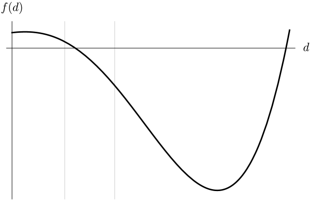
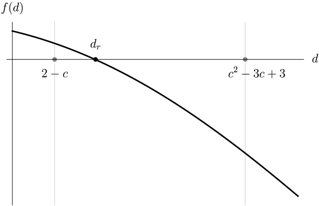
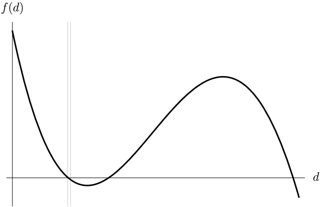
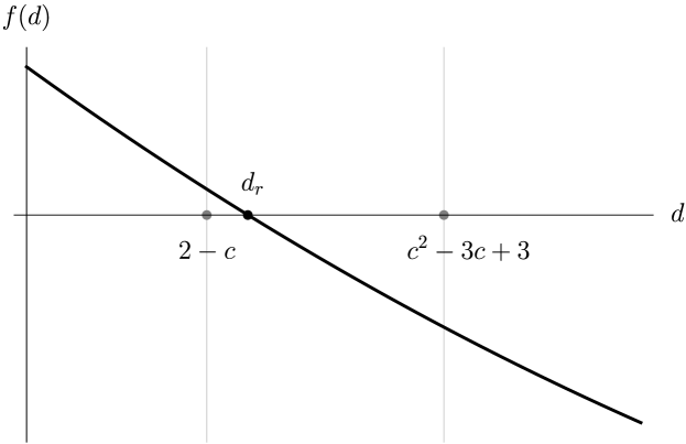
Figure 1: Two characteristic graphs of $f$ (left) and the zoom of their particular segments between two gray vertical lines involving the optimal parameter $d_{r}$ (right). Note that in the neighborhood of $d_{r}$ the graph of $f$ can be either convex or concave.

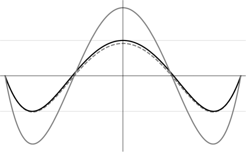
Figure 2: Graphs of the radial error $\phi_{2,0}$ and simplified radial error $\psi_{2,0}$ in the case of the parabolic $G^{0}$ interpolation with $\varphi=\pi/2$. The black graph is the optimal radial error $\phi_{2,0}$, the gray one is the optimal simplified radial error $\psi_{2,0}$ and the gray dashed is the radial error for the optimal parameter $d_{s}$ according to the simplified radial error. Observe that the minima of the gray dashed graph are smaller than the minima of the black one.

$$\begin{array}[]{|c|r|r|r|r|}\hline\cr\vrule\lx@intercol\hfil\varphi\hfil\lx@intercol\vrule\lx@intercol&\vrule\lx@intercol\hfil d_{r}\hfil\lx@intercol\vrule\lx@intercol&\vrule\lx@intercol\hfil\phi_{2,0}\hfil\lx@intercol\vrule\lx@intercol&\vrule\lx@intercol\hfil d_{s}\hfil\lx@intercol\vrule\lx@intercol&\vrule\lx@intercol\hfil\phi_{2,0}\hfil\lx@intercol\vrule\lx@intercol\\ \hline\cr\pi/2&2.21535&1.07676\times 10^{-1}&2.19737&1.09554\times 10^{-1}\\ \hline\cr\pi/3&1.54728&2.36383\times 10^{-2}&1.54643&2.37668\times 10^{-2}\\ \hline\cr\pi/4&1.30843&7.76732\times 10^{-3}&1.30834&7.78280\times 10^{-3}\\ \hline\cr\pi/6&1.13713&1.57677\times 10^{-3}&1.13712&1.57746\times 10^{-3}\\ \hline\cr\pi/8&1.07713&5.03728\times 10^{-4}&1.07713&5.03800\times 10^{-4}\\ \hline\cr\pi/12&1.03427&1.00191\times 10^{-4}&1.03427&1.00194\times 10^{-4}\\ \hline\cr\end{array}$$

Table 1: The table of optimal parameters $d_{r}$ according to the radial error $\phi_{2,0}$ and optimal parameters $d_{s}$ according to the simplified radial error $\psi_{2,0}$ for several different inner angles $2\varphi$ of a circular arc $\boldsymbol{c}$. In the last column the values of the radial error $\phi_{2,0}$ with respect to $d_{s}$ are shown. It is clearly seen that optimal parameters tend to each other when $\varphi\to 0$ but they are not the same.

The parabolic $G^{0}$ interpolation is just a special case with $k=n-2$. Note that for $n\geq 2$ the class ${\mathcal{G}}_{n}^{n-2}$ is a one-parametric family of $G^{n-2}$ polynomial interpolants of degree $n$ which will now be studied in detail.

4 Analysis of $\psi_{n,n-2}$

We have seen in the previous section that the analysis of the optimal parabolic $G^{0}$ interpolant related to the radial error leads to the analysis of the quartic polynomial (5). It is expected that the problem becomes more and more complicated for higher degrees $n$. Thus an alternative way of the analysis should be followed.
The symmetry and the restriction to $k=n-2$ imply that a one-parametric family of interpolants has to be studied. The existence and possible uniqueness of the optimal interpolant in this case has not been proven yet. It is a natural cornerstone for the study of the multi-parameter family of interpolants which will be our future work. We will see that it is basically enough to study the simplified radial error $\psi_{n,n-2}$, since its properties can be used to prove similar properties of the radial error $\phi_{n,n-2}$. The simplified radial error $\psi_{n,n-2}$ becomes

(6) $$\psi_{n,n-2}(t)=:\psi_{n}(t,d)=(t^{2}-1)^{n-1}q_{n}(t,d),$$

where $d$ is the parameter arising from the $G^{n-2}$ interpolation and $q_{n}(\cdot,d)$ is an even quadratic polynomial (see, e.g., [16]). Recall again that $q_{n}$ depends also on $\varphi$, which will not be explicitly written. Let us first observe the following general result.

Lemma 4.1.

Let $\theta_{i}(t)=(t^{2}-1)^{m}r_{i}(t)$, where $r_{i}$ is an even quadratic polynomial, $i=1,2$. If $r_{1}(0)<r_{2}(0)$ and $r_{1}(1)\leq r_{2}(1)$, then

1. $\theta_{1}(t)>\theta_{2}(t)$ for all $t\in(-1,1)$, provided $m$ is an odd number,

2. $\theta_{1}(t)<\theta_{2}(t)$ for all $t\in(-1,1)$, provided $m$ is an even number.

Proof 4.2.

Let us prove only the first part of the lemma since the proof for the other one is similar. For an odd $m$ we observe that $(t^{2}-1)^{m}<0$ for all $t\in(-1,1)$. By assumption we have $r_{1}(0)<r_{2}(0)$ and $r_{1}(1)\leq r_{2}(1)$. If there is $\tau\in(-1,1)$ such that $r_{1}(\tau)\geq r_{2}(\tau)$, the even quadratic polynomials $r_{1}$ and $r_{2}$ must have at least four intersections on $[-1,1]$ which is a contradiction. Thus $r_{1}(t)<r_{2}(t)$ for all $t\in(-1,1)$ and consequently $\theta_{1}(t)>\theta_{2}(t)$ for all $t\in(-1,1)$.

The last lemma is crucial in the proof of the existence and the uniqueness of the best $G^{n-2}$ interpolants with respect to the radial error. First note that it implies that two graphs of the simplified radial error Eq. 6 can not intersect on $(-1,1)$ for two different values $d_{1}$ and $d_{2}$, provided that $q_{n}(0,d_{1})\neq q_{n}(0,d_{2})$ and

(7) $$(q_{n}(0,d_{1})-q_{n}(0,d_{2}))(q_{n}(1,d_{1})-q_{n}(1,d_{2}))\geq 0.$$

The last relation also implies that the same is true for the graphs of the radial error $\phi_{n,n-2}(t,d)=:\phi_{n}(t,d)=\sqrt{\psi_{n}(t,d)+1}-1$ (see Fig. 2). By [2] the error function of the best interpolant must alternate three times, i.e., it must have the unique zero $\tau^{*}\in(0,1)$ which implies the smallest possible alternations. The construction of such an interpolant relies on the following facts:

• There exists an interval $I_{n}\subseteq\mathbb{R}$ such that for any $\tau\in(0,1)$ the equation $q_{n}(\tau,d)=0$ has the unique solution $d\in I_{n}$. If there is another solution $d^{\prime}\not\in I_{n}$ of the same equation, then $d$ must induce better interpolant than $d^{\prime}$.

• The functions $q_{n}(0,\cdot)$ and $q_{n}(1,\cdot)$ are both increasing or both decreasing functions on $I_{n}$ and the first one must be injective.

This suggests the following algorithm for finding $\tau^{*}$ and consequently the best interpolant:
Choose an arbitrary small $\epsilon>0$ and set $\tau_{l}:=0$, $\tau_{r}:=1$. Let $\tau=\tfrac{1}{2}(\tau_{l}+\tau_{r})$ and let $d_{\tau}\in I_{n}$ be the unique solution of the equation $q_{n}(\tau,d)=0$ (property (P1)). If $\max_{t\in[0,1]}\phi_{n}(t,d_{\tau})>|\min_{t\in[0,1]}\phi_{n}(t,d_{\tau})|$, then set $\tau_{l}=\tau$, else set $\tau_{r}=\tau$ (see Fig. 3). Repeat this procedure until $\left|\max_{t\in[0,1]}\phi_{n}(t,d_{\tau})+\min_{t\in[0,1]}\phi_{n}(t,d_{\tau})\right|\leq\epsilon$.
This is basically a method of bisection, but since we are interested in finding an interpolant which alternates, the procedure can be seen as a kind of very well known Remes algorithm ([12],[13],[14]). Observe that the same algorithm works also with the simplified error $\psi_{n}$.

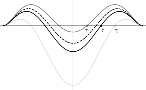
Figure 3: Graphs of $\phi_{n}(\cdot,d_{\tau})$, $\phi_{n}(\cdot,d_{\tau_{l}})$ and $\phi_{n}(\cdot,d_{\tau_{r}})$. The graph of $\phi_{n}(\cdot,d_{\tau^{*}})$ is dashed.

In the following sections we shall see that the above properties of the polynomial $q_{n}$ can be proven at least for $n=2,3,4,5$. Consequently the existence and the construction of the best geometric $G^{n-2}$ interpolant according to the radial error follows.

5 Parabolic $G^{0}$ case revisited

The parabolic $G^{0}$ case was already considered in Section 3. Here we use the approach described in the previous section. Recall that the control points of the $G^{0}$ interpolant are $\boldsymbol{b}_{0}=(c,-s)^{T}$, $\boldsymbol{b}_{1}=(d,0)^{T}$ and $\boldsymbol{b}_{2}=(c,s)^{T}$. The corresponding simplified error function is $\psi_{2}(t,d)=(t^{2}-1)q_{2}(t,d)$ and it is easy to verify that

$$q_{2}(t,d)=\frac{1}{4}\left((d-c)^{2}t^{2}-(d+c)^{2}+4\right).$$

Lemma 5.1.

For every $\tau\in[0,1)$ there exists the unique parameter $d_{\tau}\in I_{2}:=(1,\infty)$ such that $q_{2}(\tau,d_{\tau})=0$.

Proof 5.2.

The lemma follows since $q_{2}(\tau,1)=\tfrac{1}{4}(1-c)(3+c+(1-c)\tau^{2})>0$ and the leading coefficient of the polynomial $q_{2}(\tau,\cdot)$ is $-\tfrac{1}{4}(1-\tau^{2})<0$.

Lemma 5.3.

The function $q_{2}(0,\cdot)$ is strictly decreasing and $q_{2}(1,\cdot)$ is decreasing on $I_{2}$.

Proof 5.4.

The result follows directly from $q_{2}(0,d)=\tfrac{1}{4}\left(4-(d+c)^{2}\right)$ and $q_{2}(1,d)=1-cd$.

Note that the above lemmas imply the properties (P1) and (P2) and the existence and the uniqueness of the best quadratic $G^{2}$ interpolant of the circular arc according to the radial error is confirmed.

6 Cubic $G^{1}$ case

The control points in this case are

$$\boldsymbol{b}_{0}=(c,-s)^{T},\quad\boldsymbol{b}_{1}=(c,-s)^{T}+d\,(s,c)^{T},\quad\boldsymbol{b}_{2}=(c,s)^{T}+d(s,-c)^{T},\quad\boldsymbol{b}_{3}=(c,s)^{T},\quad d>0,$$

and the corresponding simplified error function is $\psi_{3}(t,d)=(t^{2}-1)^{2}q_{3}(t,d)$, where

$$q_{3}(t,d)=\frac{1}{16}\left((3dc-2s)^{2}t^{2}+(3ds+4c)^{2}-16\right).$$

Lemma 6.1.

For every $\tau\in(0,1)$ there exists the unique parameter $d_{\tau}\in I_{3}:=(0,\infty)$ such that $q(\tau,d_{\tau})=0$.

Proof 6.2.

Since $q_{3}(\tau,\cdot)$ has a positive leading coefficient $\tfrac{9}{16}(s^{2}+c^{2}\tau^{2})$ and $q_{3}(\tau,0)=-\tfrac{1}{4}s^{2}(4-\tau^{2})<0$, there exists the unique $d_{\tau}>0$ such that $q_{3}(\tau,d_{\tau})=0$.

Lemma 6.3.

The functions $q_{3}(0,\cdot)$ and $q_{3}(1,\cdot)$ are both strictly increasing functions of $d\in I_{3}$.

Proof 6.4.

Lemma follows from $q_{3}(0,d)=\tfrac{1}{16}\left((3ds+4c)^{2}-16\right)$ and $q_{3}(1,d)=\tfrac{3}{16}\left(3d^{2}+4scd-4s^{2}\right)$.

The proof of the existence and the uniqueness of the optimal cubic $G^{1}$ interpolant of the circular arc is thus confirmed. An example for the inner angle $\tfrac{\pi}{2}$ together with the corresponding radial error is in Fig. 4.

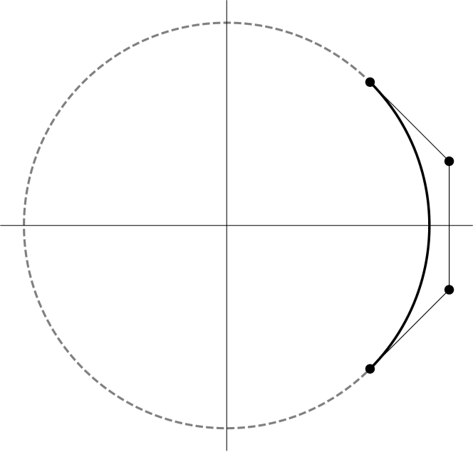
Figure 4: Graphs of the best cubic $G^{1}$ interpolant (left, solid black) of the circular arc given by the inner angle $\tfrac{\pi}{2}$ (left, dashed gray) and the corresponding radial error (right).

7 Quartic $G^{2}$ case

Since we are dealing with $G^{2}$ interpolation, the corresponding control points of the interpolant $\boldsymbol{p}_{4}$ read as

$$\boldsymbol{b}_{0}=(c,-s)^{T},\ \boldsymbol{b}_{1}=(c,-s)^{T}+\frac{\sqrt{3}}{2}\sqrt{1-c\,d}\,(s,c)^{T},\ \boldsymbol{b}_{2}=\left(d,0\right)^{T},\ \boldsymbol{b}_{3}=(c,s)^{T}+\frac{\sqrt{3}}{2}\sqrt{1-c\,d}\,(s,-c)^{T},\ \boldsymbol{b}_{4}=(c,s)^{T},$$

$d\in\mathbb{R}$, and the simplified error function is $\psi_{4}(t,d)=(t^{2}-1)^{3}q_{4}(t,d)$, where

$$q_{4}(t,d) =\frac{1}{64}\left(\left(12-3c^{2}-30cd+12c^{3}d+9d^{2}+12\sqrt{3}cs\sqrt{1-cd}-12\sqrt{3}sd\sqrt{1-cd}\right)t^{2}\right.$$

(8) $$\left.+52-13c^{2}-12c^{3}d-9d^{2}-12\sqrt{3}sd\sqrt{1-cd}-2c\left(9d+10\sqrt{3}s\sqrt{1-cd}\right)\right).$$

Note that due to the square root involved we must consider the restriction of the unknown parameter $d<1/c$. Let us define $a_{4}:=\frac{\sqrt{3}}{3}s\left(c^{2}+\sqrt{3}(1-c)\right)$ and $b_{4}:=\frac{\sqrt{3}}{3}s\left(\sqrt{3+c^{2}}-c\right)$. Observe that $0<a_{4}<b_{4}<1$ and define $J_{4}:=\left(a_{4},b_{4}\right)$. If $c\neq 0$ then let $I_{4}:=\left(\frac{1-b_{4}^{2}}{c},\frac{1-a_{4}^{2}}{c}\right)$ else $I_{4}:=\left(\tfrac{2}{\sqrt{3}},2\right)$ which can be obtained by taking the limit $c\to 0$. Observe that $q_{4}(t,\cdot)$ is an irrational function for $0<c<1$ but with the new variable $x=\sqrt{1-cd}$ the function $r_{4}(t,x):=q_{4}(t,\frac{1-x^{2}}{c})$ becomes a polynomial. Some of its obvious properties are given by the following lemma.

Lemma 7.1.

For every $t\in(0,1)$ the function $r_{4}(t,\cdot)$

• is a quartic polynomial.

• is increasing on $J_{4}$ if and only if $q_{4}(t,\cdot)$ is decreasing on $I_{4}$.

• has always four zeros, precisely one on each of the intervals $(-\infty,-1)$, $(-1,a_{4})$, $J_{4}$ and $(1,\infty)$.

Proof 7.2.

The first two properties are obvious. To see the third one (see Fig. 5), first observe that the leading coefficient of $r_{4}(t,\cdot)$ is $lc(t)=-\frac{9}{64c^{2}}(1-t^{2})$ and it is obviously negative.

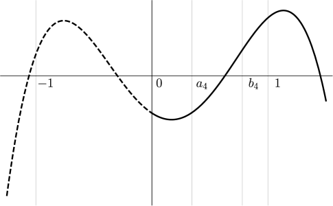
Figure 5: A characteristic graph of $r_{4}(t,\cdot)$.

A straightforward calculation reveals that

$$r_{4}(t,-1) =\frac{1}{64}\left(39+8\sqrt{3}cs+9t^{2}+12\sqrt{3}cs\left(1-t^{2}\right)+\left(1-c^{2}\right)\left(13+3t^{2}\right)\right)>0,$$

$$r_{4}(t,b_{4}) =\frac{1}{4}\left(1-c^{2}\right)\left(c\sqrt{3+c^{2}}-1-c^{2}\right)^{2}>0,$$

$$r_{4}(t,1) =\frac{1}{64}\left(52+12t^{2}+4\sqrt{3}cs\left(-5+3t^{2}\right)-c^{2}\left(13+3t^{2}\right)\right)\geq\frac{1}{64}\left(52-20\sqrt{3}-16\right)>0.$$

Since $lc(t)<0$ the property (iii) will follow if we verify $r_{4}(t,a_{4})<0$. In order to do this let us first observe that

(9) $$r_{4}(t,a_{4})=-\frac{1}{64}(1-c)^{3}(1+c)s_{4}(t),$$

where $s_{4}$ is an even quadratic polynomial. It is also quite easy to verify

$$s_{4}(0) =\left(4-2\left(1+\sqrt{3}\right)c^{2}\right)^{2}+12\left(2+\sqrt{3}\right)c^{3}(1-c)+20\left(\sqrt{3}-1\right)c\left(1-c^{3}\right)$$

$$+\left(4\left(7-4\sqrt{3}\right)+c^{2}\right)\left(1-c^{4}\right)+20\left(2\sqrt{3}-3\right)+2\left(5-2\sqrt{3}\right)c^{3}+2\left(1+2\sqrt{3}\right)c^{5}>0,$$

$$s_{4}(1) =2\left(\left(7-4\sqrt{3}\right)\left(64+40\sqrt{3}-7c\right)+c\left(3-2\sqrt{3}c\right)^{2}+c^{3}+c^{3}\left(3\sqrt{3}-2-2c\right)^{2}\right)>0,$$

and the proof of the lemma is complete.

Lemma 7.3.

For every $\tau\in(0,1)$ there exists the unique parameter $d_{\tau}\in I_{4}$ such that $q_{4}(\tau,d_{\tau})=0$.

Proof 7.4.

If $0<c<1$, the result follows directly from the previous lemma. If $c=0$ then $I_{4}=\left(\frac{2}{\sqrt{3}},2\right)$, $q_{4}(\tau,\cdot)$ is a quadratic polynomial with $q_{4}(\tau,\frac{2}{\sqrt{3}})q_{4}(\tau,2)=-\frac{1}{32}\left(6\sqrt{3}-8+3\left(2-\sqrt{3}\right)\left(1-\tau^{2}\right)\right)<0$ and the result of the lemma follows.

Since $q_{4}(t,d)=r_{4}(t,\sqrt{1-cd})$, each nonnegative zero of $r_{4}(t,\cdot)$ implies one zero of $q_{4}(t,\cdot)$. Thus by Lemma 7.1 $q_{4}(t,\cdot)$ might have two or three zeros. But the next lemma reveals that the one on $I_{4}$ provides the best approximant.

Lemma 7.5.

Let $d_{\tau}^{*}$ be the unique solution of $q_{4}(\tau,d)=0$ on $I_{4}$. If $d_{\tau}$ is any other solution of the same equation then the absolute value of the leading coefficient of $q_{4}(\cdot,d_{\tau})$ is bigger than the absolute value of the leading coefficient of $q_{4}(\cdot,d_{\tau}^{*})$.

Proof 7.6.

If $c=0$ then $I_{4}=\left(\frac{2}{\sqrt{3}},2\right)$ and $q_{4}(\tau,\cdot)$ is a quadratic polynomial with the leading coefficient $-\tfrac{9}{64}(1-\tau^{2})<0$. Furthermore, $q_{4}(\tau,0)=\tfrac{1}{16}\left(13-3\tau^{2}\right)>0$ thus the additional solution $d_{\tau}$ of $q_{4}(\tau,d)=0$ is negative. Since the leading coefficient $lc(d)=\frac{3}{64}\left(2-\sqrt{3}d\right)^{2}$ of $q_{4}(\cdot,d)$ is nonnegative, increasing on $(\tfrac{2}{\sqrt{3}},\infty)$ and decreasing elsewhere, we have $lc(d_{\tau})>lc(0)=\tfrac{3}{16}>\tfrac{3}{8}(2-\sqrt{3})=lc(2)>lc(d_{\tau}^{*})$.
Let us assume now that $0<c<1$. Denote by $x_{\tau}^{*}=\sqrt{1-cd_{\tau}^{*}}$ the unique solution of $r_{4}(\tau,x)=0$ on $J_{4}$ and by $x_{\tau}=\sqrt{1-cd_{\tau}}$ any other solution of the same equation. The leading coefficient $lc$ of the polynomial $r_{4}(\cdot,x)$ is

$$lc(x)=\frac{1}{64c^{2}}\left(9x^{4}+12\sqrt{3}csx^{3}-6\left(3-5c^{2}+2c^{4}\right)x^{2}-12\sqrt{3}cs^{3}x+9s^{4}\right).$$

It can be verified that $lc\geq 0$ with two double zeros $b_{4}^{-}=-\frac{\sqrt{3}}{3}s(\sqrt{3+c^{2}}+c)$ and $b_{4}$, and a unique local maximum at $-\tfrac{cs}{\sqrt{3}}$ (see Fig. 6). Thus $lc$ is decreasing on $[0,b_{4})$ and increasing on $(b_{4},\infty)$.

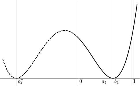
Figure 6: A characteristic graph of the leading coefficient of $r_{4}(\cdot,d)$. It is non-negative with the double zeros at $b_{4}^{-}$ and at $b_{4}$.

The proof of the lemma will be complete if we show $lc(x_{\tau}^{*})<lc(x_{\tau})$. If $x_{\tau}<a_{4}$ then the result follows from the fact that $lc$ decreases on $[0,b_{4})$. If $x_{\tau}>b_{4}$, then $x_{\tau}>1$ by Lemma 7.1 and it is enough to verify that $lc(1)\geq lc(a_{4})$. Because

$$lc(1)-lc(a_{4}) =c\left(4\sqrt{3}-9+4c^{2}\right)^{2}+12\sqrt{3}c\sqrt{1-c^{2}}+\left(24\sqrt{3}-36\right)(1-c)+3\left(28\sqrt{3}-43\right)c(1-c)$$

$$+\left(3+4\sqrt{3}\right)c^{2}(1-c)+\left(3+4\sqrt{3}\right)c^{3}(1-c)+5\left(20\sqrt{3}-29\right)c^{4}(1-c)+\left(76\sqrt{3}-129\right)c^{5}(1-c)$$

$$+\left(28\sqrt{3}-47\right)c^{6}(1-c)+\left(28\sqrt{3}-39\right)c^{7}(1-c)+\left(36\sqrt{3}-59\right)c^{8}(1-c)+\left(40\sqrt{3}-63\right)c^{9}(1-c)$$

$$+8\left(5\sqrt{3}-8\right)c^{10}>0,$$

the proof of the lemma is complete.

From the last two lemmas the property (P1) follows. In order to confirm also the property (P2), we additionally have to prove the following lemma.

Lemma 7.7.

The functions $q_{4}(0,\cdot)$ and $q_{4}(1,\cdot)$ are strictly decreasing on $I_{4}$.

Proof 7.8.

Let us first observe that for $c=0$ we have $q_{4}(0,d)=\frac{1}{64}\left(52-12\sqrt{3}d-9d^{2}\right)$ and $q_{4}(1,d)=1-\frac{3\sqrt{3}d}{8}$ which are obviously strictly decreasing on $I_{4}$.
If $0<c<1$ we again consider the function $r_{4}(t,x)=q_{4}\left(t,\frac{1-x^{2}}{c}\right)$. By Lemma 7.1 the proof will be complete if we verify that $r_{4}(0,\cdot)$ and $r_{4}(1,\cdot)$ are strictly increasing on $J_{4}$.
Recall that $r_{4}(t,\cdot)$ is a quartic polynomial with the leading coefficient $-\frac{9}{64c^{2}}\left(1-t^{2}\right)$. Consequently, $f_{0}(x):=\frac{dr_{4}}{dx}(0,x)$ is a cubic polynomial with the negative leading coefficient and $f_{1}(x):=\frac{dr_{4}}{dx}(1,x)$ is quadratic with the positive leading coefficient $\tfrac{9\sqrt{3}s}{8c}$. So, it suffices to show that $f_{i}(0)<0$, $f_{i}(a_{4})>0$ and $f_{i}(1)>0$ for $i=0,1$. By straightforward computations we have

$$f_{0}(0)=-\frac{\sqrt{3}\left(3+5c^{2}\right)s}{16c}<0,\quad f_{1}(0)=-\frac{\sqrt{3}\left(3+c^{2}\right)s}{8c}<0,\quad$$

and

$$f_{0}(1)=\frac{9c+6c^{3}+\sqrt{3}s(6-5c^{2})}{16c}>0,\quad f_{1}(1)=\frac{12c+\sqrt{3}s\left(6-c^{2}\right)}{8c}>0.$$

In order to show $f_{i}(a_{4})>0$, $i=0,1$, we observe that $f_{0}(a_{4})=\frac{s(1-c)}{16c}\,g_{0}(c)$ and $f_{1}(a_{4})=\frac{\sqrt{3}s(1-c)}{8c}g_{1}(c)$, where

$$g_{0}(c) =6\left(3+\sqrt{3}\right)+9\left(1-2\sqrt{3}\right)c-5\sqrt{3}c^{2}+2\left(3+8\sqrt{3}\right)c^{3}-2\left(9+4\sqrt{3}\right)c^{4}+\left(9+2\sqrt{3}\right)c^{5}-\sqrt{3}c^{6},$$

$$g_{1}(c) =6-4\left(3-\sqrt{3}\right)c-\left(13-6\sqrt{3}\right)c^{2}+9c^{3}+\left(3-6\sqrt{3}\right)c^{4}+3c^{5}.$$

Let us write $g_{0}=g_{01}+g_{02}+g_{03}$, where

$$g_{01}(c) =6\left(3+\sqrt{3}\right)-9\left(-1+2\sqrt{3}\right)c,$$

$$g_{02}(c) =-5\sqrt{3}c^{2}+\left(9+\sqrt{3}\right)c^{5},$$

$$g_{03}(c) =c^{3}\left(2\left(3+8\sqrt{3}\right)-2\left(9+4\sqrt{3}\right)c+\sqrt{3}c^{2}(1-c)\right).$$

It is now easy to verify $g_{01}(c)>27-12\sqrt{3}\approx 6.22$, $g_{02}(c)\geq-3\sqrt[6]{3^{5}}\sqrt[3]{\left(\frac{2}{9+\sqrt{3}}\right)^{2}}\approx-2.45$, $g_{03}(c)>0$, thus $g_{0}(c)>0$ and consequently $f_{0}(a_{4})>0$. Similarly, let us write $g_{1}=g_{11}+g_{12}$, where

$$g_{11}(c)=6-4\left(3-\sqrt{3}\right)c\quad{\rm and}\quad g_{12}(c)=c^{2}\left(-13+6\sqrt{3}+9c+\left(3-6\sqrt{3}\right)c^{2}+3c^{3}\right).$$

Again, we can bound $g_{11}(c)>4\sqrt{3}-6\approx 0.93$ and $g_{12}(c)>-0.05$, thus $g_{1}(c)>0$ and so $f_{1}(a_{4})>0$. Note that the exact value of $g_{12}$ can be given in a closed form but it is to complicated to be written here.

From the previous proofs the properties (P1) and (P2) follow also for the quartic $G^{2}$ case. Let us demonstrate the results by some examples. Consider the quartic case with $\varphi=\pi/4$. According to Lemma 7.3, Lemma 7.5 and Lemma 7.7, there is the unique best $G^{2}$ interpolant of the circular arc with respect to the radial error. From the above proofs of the lemmas it can be seen that there might be another $G^{2}$ interpolant for which the radial error alternates three times. More precisely, some analysis based on numerical computations actually reveals that this happens for all angles $\varphi<\arccos{3/5}$. Indeed, such an interpolant exists but its radial error is much bigger that the error of the optimal interpolant. Numerical experiments indicate that it is quite difficult to find the best interpolant numerically directly by constructing an appropriate equation for the unknown $d$. The bisection algorithm described in Section 4 should be used instead. The results are shown in Fig. 7.

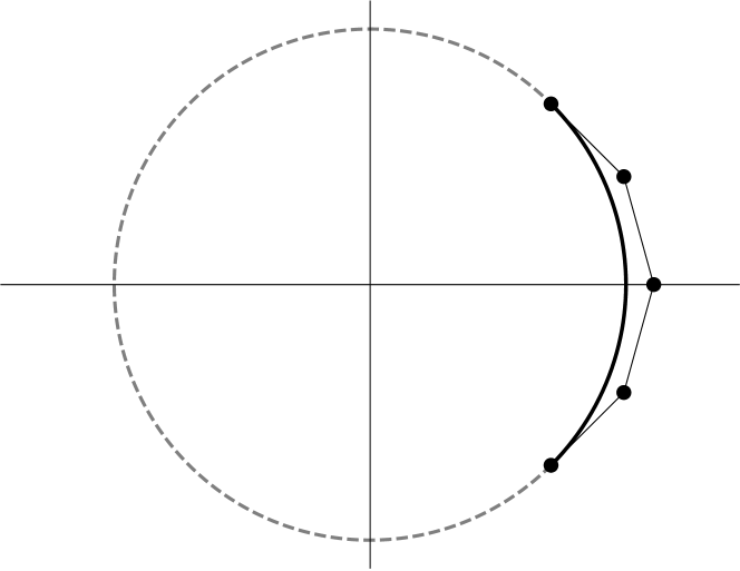
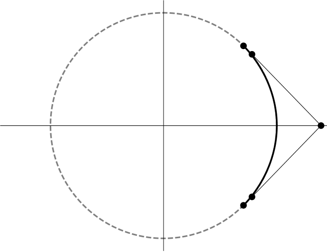
Figure 7: Graphs of two quartic $G^{2}$ interpolants (solid black) of the circular arc given by the inner angle $\pi/2$ (dashed gray). The best one is on the left. The maximum of its radial error is approximately $2.5\times 10^{-6}$. The interpolant on the right has alternating radial error too, but its maximal value is approximately $2\times 10^{-3}$ and it is much bigger than for the optimal interpolant.

8 Quintic $G^{3}$ case

Here we consider the $G^{3}$ interpolation which implies the control points

$$\boldsymbol{b}_{0} =(c,-s)^{T},\quad\boldsymbol{b}_{1}=(c,-s)^{T}+d(s,c)^{T},\quad\boldsymbol{b}_{2}=\left(\frac{5d(4-5d^{2})c+4(2+5d^{2})s}{4(5d+2sc)},-\frac{5d((4-5d^{2})s-6dc)}{4(5d+2sc)}\right)^{T},$$

$$\boldsymbol{b}_{3} =\left(\frac{5d(4-5d^{2})c+4(2+5d^{2})s}{4(5d+2sc)},\frac{5d((4-5d^{2})s-6dc)}{4(5d+2sc)}\right)^{T},\quad\boldsymbol{b}_{4}=(c,s)^{T}+d(s,-c)^{T}\quad\boldsymbol{b}_{5}=(c,s)^{T},$$

with $d<0$ due to the $G^{1}$ continuity. The corresponding simplified error function is $\psi_{5}(t,d)=(t^{2}-1)^{4}q_{5}(t,d)$, where $q_{5}(\cdot,d)$ is a quadratic polynomial with rational coefficients in $d$. Let us define

$$0<\alpha_{5}:=\frac{2s}{5}\leq a_{5}:=\frac{16s}{25+15c}<b_{5}:=\frac{2s}{3+2c}<\beta_{5}:=\frac{4s}{5(1+c)}<1,$$

and $I_{5}:=(a_{5},b_{5})$. Similarly as in the previous cases, we will confirm the properties (P1) and (P2) (see Fig. 8 for better understanding the proofs in the following).

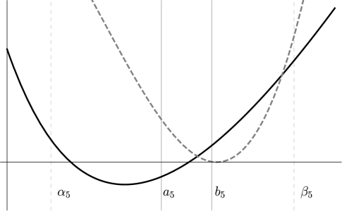
Figure 8: A characteristic graph of $q_{5}(\cdot,d)$ (black) and its leading coefficient $lc$ (gray dashed).

Let us first consider the behavior of the leading coefficient $lc$ of $q_{5}(\cdot,d)$ which is of the form $lc(d)=(r(d))^{2}$, where

$$r(d)=\frac{125sd^{3}+100cd^{2}-20s(3+c^{2})d+16cs^{2}}{32(5d+2sc)}.$$

Lemma 8.1.

The leading coefficient $lc$ of the polynomial $q_{5}(\cdot,d)$ is a decreasing function of the variable $d$ on $\left(\alpha_{5},b_{5}\right)\supset I_{5}$ and it is an increasing function on $\left(\beta_{5},\infty\right)$.

Proof 8.2.

Recall that $lc(d)=(r(d))^{2}$. The denominator of the derivative

$$r^{\prime}(d)=\frac{5(125sd^{3}+25c(2+3s^{2})d^{2}+40sc^{2}d-4cs^{2}(5+c^{2}))}{16(5d+2sc)^{2}}$$

is positive and the nominator is an increasing function of the variable $d\in[\alpha_{5},\infty)$. Since $r^{\prime}(\alpha_{5})=\tfrac{5(1-c)}{8(1+c)^{2}}(1+c+2c^{2})>0$, the function $r$ is increasing on $(\alpha_{5},\infty)$. Since

$$r\left(b_{5}\right)=-\frac{(1-c)^{2}(5-2c+2c^{2})s}{4(3+2c)^{2}(5+3c+2c^{2})}<0\quad{\rm and}\quad r\left(\beta_{5}\right)=\frac{(1-c)^{2}s}{4(1+c)(2+c+c^{2})}>0.$$

the result of the lemma follows.

Lemma 8.3.

For any $t\in(0,1)$ the function $q_{5}(t,\cdot)$ is a convex function on the interval $(0,\beta_{5})\subset(0,1)$.

Proof 8.4.

Let us define $g(x)=q_{5}(t,\beta_{5}x)$. Then the function $q_{5}(t,\cdot)$ is convex on the interval $(0,\beta_{5})$ if and only if the function $g$ is convex on the interval $(0,1)$. Since

$$g^{\prime\prime}(x)=\frac{1-c}{8(1+c)^{2}\left(2x+c+c^{2}\right)^{4}}\left(\sum_{j=0}^{5}a_{j}(t)x^{j}(1-x)+a_{6}(t)x^{6}\right),$$

for some even quadratic polynomials $a_{j}$, it is enough to show that $a_{j}(0)>0$ and $a_{j}(1)>0$ for $j=0,\ldots,6$. The latter can be easily checked and details will be omitted here.

Lemma 8.5.

For any $t\in(0,1)$ the function $\psi_{5}(t,\cdot)$ has exactly two zeros on the interval $(0,\beta_{5})$. One is on the interval $(\alpha_{5},a_{5})$ and the other one is on the interval $I_{5}$.

Proof 8.6.

By the previous lemma $\psi_{5}(t,\cdot)$ has at most two zeros on the interval $(0,\beta_{5})$. The result of the lemma follows since

$$\psi_{5}\left(t,\alpha_{5}\right) =\frac{(1-c)^{5}(1-t^{2})^{4}t^{2}}{16(1+c)}>0,$$

$$\psi_{5}\left(t,a_{5}\right) =-\frac{(1+c)(1-c)^{4}(1-t^{2})^{4}}{1024(5+3c)^{4}(8+5c+3c^{2})^{2}}$$

$$\times(48(15925+4065c+1338c^{2}-3846c^{3}-1071c^{4}-27c^{5})-64(1-c)(44+3c+9c^{2})^{2}t^{2})<0,$$

$$\psi_{5}\left(t,b_{5}\right) =\frac{(1+c)(1-c)^{4}(1-t^{2})^{4}}{64(3+2c)^{4}(5+3c+2c^{2})^{2}}(16c(180+169c+123c^{2}+27c^{3}+c^{4})+4(1-c)(5-2c+2c^{2})^{2}t^{2})>0.$$

We are finally ready to confirm the properties (P1) and (P2).

Lemma 8.7.

The functions $q_{5}(0,\cdot)$ and $q_{5}(1,\cdot)$ are strictly increasing on $I_{5}$. For every $\tau\in(0,1)$ there exists the unique solution $d_{\tau}$ of the equation $q_{5}(\tau,d)=0$ on the interval $I_{5}$. For any other solution $d$ of the equation $q_{5}(t,d)=0$, we have $lc(d)>lc(d_{t})$.

Proof 8.8.

Let us first prove the monotonicity of $q_{5}(0,d)$. Note that $q_{5}(0,d)=\psi_{5}(0,d)=(f(d))^{2}-1$, where

$$f(d)=\frac{8(5+3c^{2})s+20c(9-c^{2})d+150sd^{2}-125cd^{3}}{32(5d+2sc)}.$$

Since $I_{5}\subset(0,1)$ and $f>0$ on $(0,1)$, it is enough to show that $f^{\prime}>0$ on $I_{5}$. The derivative $f^{\prime}$ can be written as $f^{\prime}(d)=\tfrac{5}{16}(5d+2sc)^{-2}g(d)$, where $g(d)=-4(5-6c^{2}+c^{4})s+60s^{2}cd+75s^{3}d^{2}-125cd^{3}$. The inequality $g(d)>0$ holds for all $d\in I_{5}$ since

$$g\left(\frac{2(1-c)s}{75+95c+30c^{2}}x+\frac{16s}{25+15c}\right)=\frac{4s^{3}(1-c)^{2}}{(3+2c)^{3}(5+3c)^{3}}\left((3+2c)^{3}(335+297c+189c^{2}+27c^{3})\right.$$

$$\left.+30(3+2c)^{2}(8+5c+3c^{2})x+3(5+2c+c^{2})(3+2c)(1-3c)x^{2}-2(1-c)cx^{3}\right)$$

$$\geq\frac{4s^{3}(1-c)^{2}}{(3+2c)^{3}(5+3c)^{3}}\left(3^{3}\,335+0-90-2\right)>0$$

for all $x\in(0,1)$.

Let us now check that the function $h=q_{5}(1,\cdot)$ is increasing on $I_{5}$. Note that

$$h^{\prime}\left(a_{5}\right) =\frac{5(1-c)^{2}s}{64(5+3c)^{3}\left(8+5c+3c^{2}\right)^{3}}$$

$$\times\left(440863+1380116c+1950998c^{2}+1731140c^{3}+984672c^{4}+368604c^{5}+80946c^{6}+8748c^{7}+729c^{8}\right)>0,$$

$$h^{\prime\prime}\left(b_{5}\right) =\frac{375(1-c)}{32(3+2c)^{2}\left(5+3c+2c^{2}\right)^{4}}$$

$$\times\left(2755+9325c+15649c^{2}+16453c^{3}+11136c^{4}+4638c^{5}+688c^{6}-356c^{7}-240c^{8}-48c^{9}\right)>0,$$

$$h^{\prime\prime\prime}\left(b_{5}\right) =-\frac{375}{16(3+2c)\left(5+3c+2c^{2}\right)^{5}s}$$

$$\times\left(650+8850c+24645c^{2}+41580c^{3}+53039c^{4}+52746c^{5}+40515c^{6}+22080c^{7}+7255c^{8}+216c^{9}\right.$$

$$\left.-1016c^{10}-480c^{11}-80c^{12}\right)<0,$$

and

$$h^{\prime\prime\prime\prime}\left(d\right)=\frac{1875}{128}\left(1+\frac{320\left(5+2c^{2}+c^{4}\right)^{2}s^{4}}{(5d+2cs)^{6}}\right)>0.$$

These imply that $h^{\prime\prime\prime}<0$, $h^{\prime\prime}>0$ and $h^{\prime}>0$ on $I_{5}$.

By Lemma 8.5, there is the unique solution $d_{\tau}\in I_{5}$ of the equation $q_{5}(\tau,d)=0$ and for any other solution $d$ we have $d<d_{\tau}$ or $d>\beta_{5}$. By Lemma 8.1, the leading coefficient $lc(d)>lc(a_{5})>lc(d_{\tau})$, provided $d<d_{\tau}$, and $lc(d)>lc(\beta_{5})$, provided $d>\beta_{5}$. Hence it is enough to show that $lc(\beta_{5})>lc(a_{5})$, which follows from

$$\sqrt{lc\left(\beta_{5}\right)}-\sqrt{lc\left(a_{5}\right)}=r(\beta_{5})-r(a_{5}) =\frac{s(1-c)^{2}}{4(1+c)(2+c+c^{2})}-\frac{s(1-c)^{2}(44+3c+9c^{2})}{4(5+3c)^{2}(8+5c+3c^{2})}$$

$$=\frac{s(1-c)^{2}\left(112+227c+182c^{2}+58c^{3}+6c^{4}-9c^{5}\right)}{4\left(1+c\right)\left(2+c+c^{2}\right)\left(5+3c\right)^{2}\left(8+5c+3c^{2}\right)}>0.$$

The following example reveals that there might be several quintic $G^{3}$ interpolants with the alternating radial error. Some of them possess quite interesting configuration of the control points (see Fig. 9).

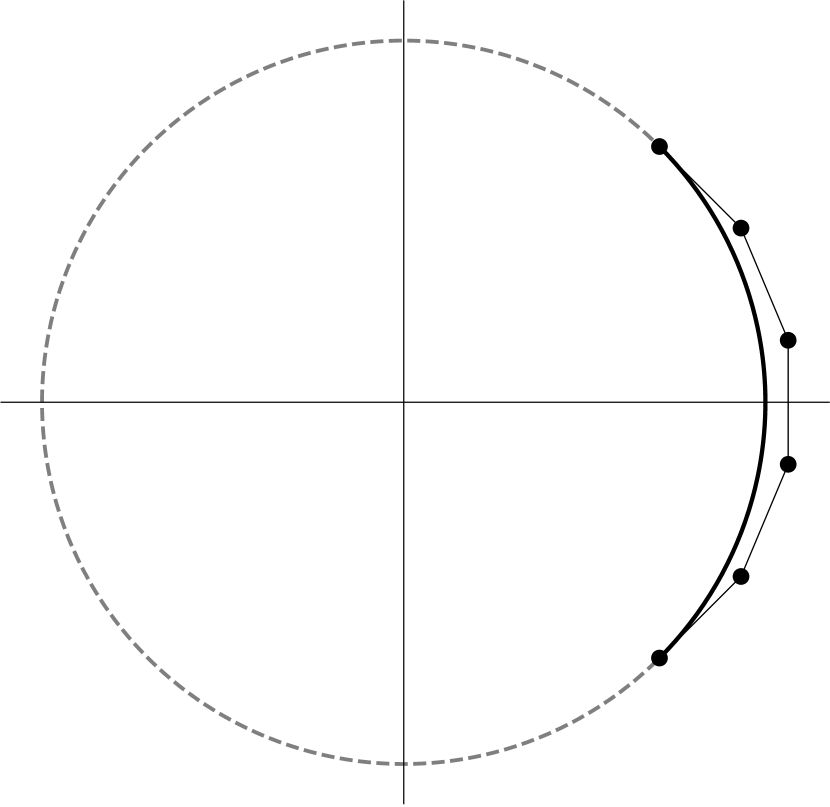
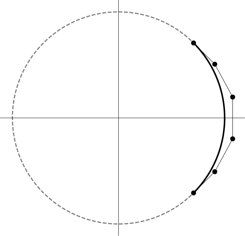
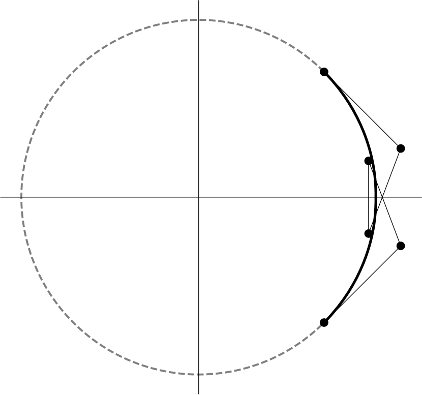
Figure 9: Graphs of quintic $G^{3}$ interpolants (solid black) of the circular arc given by the inner angle $\pi/2$ (dashed gray). The left one is the best interpolant with the maximum of the radial error approximately $2\times 10^{-8}$. The middle one and one on the right have an alternating radial error too. But the values of their radial errors are approximately $2\times 10^{-6}$ for the middle one, and $8\times 10^{-4}$ for the one on the right.

9 Conclusion

In this paper a new approach to study the circular arc approximation by parametric polynomials via the geometric interpolation has been considered. The existence and the uniqueness of the best parametric polynomial of some particular degree and order of geometric smoothness were confirmed for the simplified radial error and also for the radial error itself. The later one is a new result which, up to our knowledge, has not been studied in the literature yet. A general iterative algorithm for the construction of the best parametric polynomial approximant was established in the case when the degree of the parametric polynomial $n$ and the order of geometric smoothness $k$ are related by $k=n-2$. The algorithm is based on a kind of bisection method, thus it is robust and leads to the desired solution for any starting point of the iteration. Since the cases $n=2,3,4,5$ have been analyzed only, one can consider the analysis of some higher degrees as a future work. But even more important is the analysis of some low degree cases for which $n-k>2$. The first step in this direction was done in [16] and in [15] but only for the simplified radial error. It is clear that the problem of finding the best geometric interpolant in the case of the radial error is much more challenging issue.

References

- [1] T. Dokken, M. Dæhlen, T. Lyche, and K. Mørken, Good approximation of circles by curvature-continuous Bézier curves, Comput. Aided Geom. Design, 7 (1990), pp. 33–41. Curves and surfaces in CAGD ’89 (Oberwolfach, 1989).
- [2] E. F. Eisele, Chebyshev approximation of plane curves by splines, J. Approx. Theory, 76 (1994), pp. 133–148.
- [3] L. Fang, Circular arc approximation by quintic polynomial curves, Comput. Aided Geom. Design, 15 (1998), pp. 843–861.
- [4] M. Goldapp, Approximation of circular arcs by cubic polynomials, Comput. Aided Geom. Design, 8 (1991), pp. 227–238.
- [5] S. Hur and T. Kim, The best cubic and quartic bézier approximations of circular arcs, J. Comput. Appl. Math., 236 (2011), pp. 1183–1192.
- [6] G. Jaklič, Uniform approximation of a circle by a parametric polynomial curve, Comput. Aided Geom. Design, 41 (2016), pp. 36–46.
- [7] G. Jaklič and J. Kozak, On parametric polynomial circle approximation, Numer. Algorithms, 77 (2017), pp. 433–450.
- [8] S.-H. Kim and Y. J. Ahn, An approximation of circular arcs by quartic Bézier curves, Comput. Aided Design, 39 (2007), pp. 490–493.
- [9] M. Knez and E. Žagar, Interpolation of circular arcs by parametric polynomials of maximal geometric smoothness, Comput. Aided Geom. Design, 63 (2018), pp. 66–77.
- [10] B. Kovač and E. Žagar, Some new quartic parametric approximants of circular arcs, Appl. Math. Comput., 239 (2014), pp. 254–264.
- [11] K. Mørken, Best approximation of circle segments by quadratic Bézier curves, in Curves and surfaces (Chamonix-Mont-Blanc, 1990), Academic Press, Boston, MA, 1991, pp. 331–336.
- [12] E. Remes, Sur la détermination des polynomes d’approximation de degré donnée, Commun. Soc. Math. Kharkov, 10 (1934).
- [13] E. Remes, Sur le calcul effectif des polynomes d’approximation de Tchebychef, C. R. Acad. Sci., 199 (1934), pp. 337–340.
- [14] E. Remes, Sur un procédé convergent d’approximations successives pour déterminer les polynomes d’approximation, C. R. Acad. Sci., 198 (1934), pp. 2063–2065.
- [15] A. Vavpetič, Optimal parametric interpolants of circular arcs, preprint.
- [16] A. Vavpetič and E. Žagar, A general framework for the optimal approximation of circular arcs by parametric polynomial curves, J. Comput. Appl. Math., 345 (2019), pp. 146–158.
- [17] Z. Xiaoming and C. Licai, Approximation of circular arcs by quartic Bézier curves, J. Comp.-Aided Design Comp. Graph., 22 (2010), p. 1094.