Partial Queries for Constraint Acquisition

Abstract

Learning constraint networks is known to require a number of membership queries exponential in the number of variables. In this paper, we learn constraint networks by asking the user partial queries. That is, we ask the user to classify assignments to subsets of the variables as positive or negative. We provide an algorithm, called QuAcq, that, given a negative example, focuses onto a constraint of the target network in a number of queries logarithmic in the size of the example. The whole constraint network can then be learned with a polynomial number of partial queries. We give information theoretic lower bounds for learning some simple classes of constraint networks and show that our generic algorithm is optimal in some cases. Finally we evaluate our algorithm on some benchmarks.

1 Introduction

Constraint programming (CP) has been more and more used to solve combinatorial problems in industrial applications. One of the strengths of CP is that it is declarative, which means that the user specifies the problem as a CP model, and the solver finds solutions. However, it appears that specifying the CP model is not that easy for non-specialists. Hence, the modeling phase constitutes a major bottleneck in the use of CP. Several techniques have been proposed to tackle this bottleneck. In Conacq.1 [7, 9, 12], the user provides examples of solutions (positive) and non-solutions (negative). Based on these positive and negative examples, the system learns a set of constraints that correctly classifies all examples given so far. This is a form of passive learning. A passive learner based on inductive logic programming is presented in [21]. This system requires background knowledge on the structure of the problem to learn a representation of the problem correctly classifying the examples. In ModelSeeker [5], the user provides positive examples to the system, which arranges each of them as a matrix and identifies constraints in the global constraints catalog ([4]) that are satisfied by particular subsets of variables in all the examples. Such particular subsets are for instance rows or columns. The candidate constraints are ranked and proposed to the user for selection. This ranking/selection combined with the representation of examples as matrices allows ModelSeeker to quickly find a good model when the problem has an underlying matrix structure. More recently, a passive learner called Arnold has been proposed [20]. Arnold takes positive examples as input and returns an integer program that accepts these examples as solutions. Arnold relies on a tensor-based language for describing polynomial constraints between multi-dimensional vectors. As in ModelSeeker, the problem needs to have an underlying matrix structure. Conacq.1 is thus the only passive learner that can learn constraints when the problem does not have a specific structure.

By contrast, in an active learner like Conacq.2 [10, 12], the system proposes examples to the user to classify as solutions or non solutions. Such questions are called membership queries [2]. In applications where we need a proof that the learning system has converged to the target set of constraints, active learning is a good candidate because it can significantly decrease the number of examples necessary to converge. For instance, a few years ago, the Normind company hired a constraint programming specialist to transform their expert system for detecting failures in electric circuits in Airbus airplanes into a constraint model in order to make it more efficient and easier to maintain. An active learner can do this by automatically interacting with the expert system. As another example, active learning was used to build a constraint model that encodes non-atomic actions of a robot (e.g., catch a ball) by asking queries of the simulator of the robot [23]. Such active learning introduces two computational challenges. First, how does the system generate a useful query? Second, how many queries are needed for the system to converge to the target set of constraints? It has been shown that the number of membership queries required to converge to the target set of constraints can be exponentially large [11, 12].

In this paper, we propose QuAcq (for Quick Acquisition), an active learner that asks the user to classify partial queries as positive or negative. Given a negative example, QuAcq is able to learn a constraint of the target constraint network in a number of queries logarithmic in the number of variables. As a result, QuAcq converges on the target constraint network in a polynomial number of queries. In fact, we identify information theoretic lower bounds on the complexity of learning constraint networks that show that QuAcq is optimal on some simple languages and close to optimal on others. One application for QuAcq would be to learn a general purpose model. In constraint programming, a distinction is made between model and data. For example, in a sudoku puzzle, the model contains generic constraints like each subsquare contains a permutation of the numbers. The data, on the other hand, gives the pre-filled squares for a specific puzzle. As a second example, in a time-tabling problem, the model specifies generic constraints like no teacher can teach multiple classes at the same time. The data, on the other hand, specifies particular room sizes, and teacher availability for a particular time-tabling problem instance. The cost of learning the model can then be amortized over the lifetime of the model. QuAcq has several advantage. First, it is the only approach ensuring the property of convergence in a polynomial number of queries. Second, as opposed to existing techniques, the user does not need to give positive examples. This might be useful if the problem has not yet been solved, so there are no examples of past solutions. Third, QuAcq learns any kind of network, whatever the constraints are organized in a specific structure or not. Fourth, QuAcq can be used when part of the network is already known from the user or from another learning technique. Experiments show that the larger the amount of known constraints, the fewer the queries required to converge on the target network.

The rest of the paper is organized as follows. Section 2 gives the necessary definitions to understand the technical presentation. Section 3 describes the differences between the algorithm presented in this paper and the version in [8]. Section 4 presents QuAcq, the algorithm that learns constraint networks by asking partial queries. In Section 5, we show that QuAcq behaves optimally on some simple languages. Section 6 presents an experimental evaluation of QuAcq. Section 7 concludes the paper.

2 Background

The learner and the user need to share some common knowledge to communicate. We suppose this common knowledge, called the vocabulary, is a (finite) set of $n$ variables $X$ and a domain $D=\{D(X_{1}),\ldots,D(X_{n})\}$, where $D(X_{i})\subset\mathbbm{Z}$ is the finite set of values for $X_{i}$. A constraint $c$ is defined by a sequence of variables $scp(c)\subseteq X$, called the constraint scope, and a relation $rel(c)$ over $\mathbbm{Z}$ specifying which sequences of $|scp(c)|$ values are allowed for the variables $scp(c)$. We will use the notation $var(c)$ to refer to the set of variables in $scp(c)$, and we abusively call it ’scope’ too when no confusion is possible. A constraint network (or simply network) is a set $C$ of constraints on the vocabulary $(X,D)$. An assignment $e_{Y}\in D^{Y}$, where $D^{Y}=\Pi_{X_{i}\in Y}D(X_{i})$, is called a partial assignment when $Y\subset X$ and a complete assignment when $Y=X$. An assignment $e_{Y}$ on a set of variables $Y\subseteq X$ is rejected by a constraint $c$ (or $e_{Y}$ violates $c$) if $var(c)\subseteq Y$ and the projection $e_{Y}[scp(c)]$ of $e_{Y}$ on the variables $scp(c)$ is not in $rel(c)$. If $e_{Y}$ does not violate $c$, it satisfies it. An assignment $e_{Y}$ on $Y$ is accepted by $C$ if and only if it does not violate any constraint in $C$. An assignment on $X$ that is accepted by $C$ is a solution of $C$. We write $sol(C)$ for the set of solutions of $C$. We write $C[Y]$ for the set of constraints in $C$ whose scope is included in $Y$, and $C_{Y}$ for the set of constraints in $C$ whose scope is exactly $Y$. We say that two networks $C$ and $C^{\prime}$ are equivalent if $sol(C)=sol(C^{\prime})$.

In addition to the vocabulary, the learner owns a language $\Gamma$ of bounded arity relations from which it can build constraints on specified sets of variables. Adapting terms from machine learning, the constraint basis, denoted by $B$, is a set of constraints built from the constraint language $\Gamma$ on the vocabulary $(X,D)$ from which the learner builds a constraint network.

The target network is a network $T$ such that $T\subseteq B$ and for any example $e\in D^{X}$, $e$ is a solution of $T$ if and only if $e$ is a solution of the problem that the user has in mind. A membership query $ASK(e)$ takes as input a complete assignment $e$ in $D^{X}$ and asks the user to classify it. The answer to $ASK(e)$ is yes if and only if $e\in sol(T)$. A partial query $ASK(e_{Y})$, with $Y\subseteq X$, takes as input a partial assignment $e$ in $D^{Y}$ and asks the user to classify it. The answer to $ASK(e_{Y})$ is yes if and only if $e_{Y}$ does not violate any constraint in $T$. It is important to observe that ”$ASK(e_{Y})$=yes ” does not mean that $e_{Y}$ extends to a solution of $T$, which would put an NP-complete problem on the shoulders of the user. A classified assignment $e_{Y}$ is called positive or negative example depending on whether $ASK(e_{Y})$ is yes or no. For any assignment $e_{Y}$ on $Y$, $\kappa_{B}(e_{Y})$ denotes the set of all constraints in $B$ that reject $e_{Y}$. We will also use $\kappa_{\Delta}(e_{Y})$ to denote the set of constraints in a given set $\Delta$ that reject $e_{Y}$.

We now define convergence, which is the constraint acquisition problem we are interested in. Given a set $E$ of (partial) examples labeled by the user yes or no, we say that a network $C$ agrees with $E$ if $C$ accepts all examples labeled yes in $E$ and does not accept those labeled no. The learning process has converged on the network $L\subseteq B$ if $L$ agrees with $E$ and for every other network $L^{\prime}\subseteq B$ agreeing with $E$, we have $sol(L^{\prime})=sol(L)$. We are thus guaranteed that $L$ is equivalent to $T$. It is important to note that $L$ is not necessarily unique and equal to $T$. This is because of redundant constraints. Given a set $C$ of constraints, a constraint $c\notin C$ is redundant wrt $C$ if $sol(C)=sol(C\cup\{c\})$. If a constraint $c$ from $B$ is redundant wrt $T$, the network $T\cup\{c\}$ is equivalent to $T$.

In the algorithms presented in the rest of the paper we will use the join operation, denoted by $\Join$. Given two sets of constraints $S$ and $S^{\prime}$, the join of $S$ with $S^{\prime}$ is the set of non-empty constraints obtained by pairwise conjunction of a constraint in $S$ with a constraint in $S^{\prime}$. That is, $S\Join S^{\prime}=\{c\land c^{\prime}\mid c\in S,c^{\prime}\in S^{\prime},c\land c^{\prime}\not\models\bot\}$. A constraint belonging to the basis $B$ will be called elementary in contrast to a constraint composed of the conjunction of several elementary constraints, which will be called conjunction. A conjunction will also sometimes be referred to as a set of elementary constraints. Given a set $S$ of conjunctions, we will use the notation $S_{p}$ to refer to the subset of $S$ containing only the conjunctions composed of at most $p$ elementary constraints. Finally, a normalized network is a network that does not contain conjunctions of constraints on any scope, that is, all its constraints are elementary.

3 QuAcq2 versus QuAcq1

A first version of QuAcq was published in [8]. From now on let us call it QuAcq1. That version was devoted to normalized constraint networks, that is, networks for which there does not exist any pair of constraints with scopes included one in the other. In addition, QuAcq1 was not taking as assumption that the target network is a subset of constraints from the basis. As a consequence, when the target network was not a subset of the basis, QuAcq1 was either learning a wrong network or was subject to a ”collapse” state. When the target network was a subset of the basis, QuAcq1 was asking redundant (i.e., useless) queries. In QuAcq2, the problem of constraint acquisition is formulated in a way that is more in line with standard concept learning [3, 24]. The target network is a subset of the constraints in the basis. As a consequence, an active learner such as QuAcq2 will always return the last possible constraint network given a set of examples already classified. It will never collapse. The second difference with QuAcq1 is that QuAcq2 does not require that the target network is normalized. QuAcq2 can learn any type of constraint network.

4 Constraint Acquisition with Partial Queries

We propose QuAcq2, a novel active learning algorithm. QuAcq2 takes as input a basis $B$ on a vocabulary $(X,D)$. It asks partial queries of the user until it has converged on a constraint network $L$ equivalent to the target network $T$. When a query is answered yes, constraints rejecting it are removed from $B$. When a query is answered no, QuAcq2 enters a loop (functions FindScope and FindC) that will end by the addition of a constraint to $L$.

4.1 Description of QuAcq2

QuAcq2 (see Algorithm 1) initializes the network $L$ it will learn to the empty set (line 1). In line 1, QuAcq2 calls function GenerateExample that computes an assignment $e_{Y}$ on a subset of variables $Y$ satisfying the constraints of $L$ that have a scope included in $Y$, but violating at least one constraint from $B$. We will see later that there are multiple ways to design function GenerateExample. If there does not exist any pair $(Y,e_{Y})$ accepted by $L$ and rejected by $B$ (i.e., GenerateExample returns $\bot$), then all constraints in $B$ are implied by $L$, and we have converged (line 1). If we have not converged, we propose the example $e_{Y}$ to the user, who will answer by yes or no (line 1). If the answer is yes, we can remove from $B$ the set $\kappa_{B}(e_{Y})$ of all constraints in $B$ that reject $e_{Y}$ (line 1). If the answer is no, we are sure that $e_{Y}$ violates at least one constraint of the target network $T$. We then call the function FindScope to discover the scope $S$ of one of these violated constraints, and the procedure FindC will learn (that is, put in $L$) at least one constraint of $T$ whose scope is in $S$ (line 1).

In : A basis $B$

Out : A learned network $L$

1 begin

2       $L\leftarrow\varnothing$;

3       while true do

4             $e_{Y}\leftarrow\texttt{Generate\-Example}(X,L,B)$;

5             if $e_{Y}=\bot$ then  return “convergence on $L$”;

6             if $ASK(e_{Y})=\textit{yes}$  then

7                   $B\leftarrow B\setminus\kappa_{B}(e_{Y})$;

8                  

9             else  $\texttt{FindC}(e_{Y},\texttt{FindScope}(e_{Y},\varnothing,Y),L)$;

10            

11      

12

Algorithm 1 QuAcq2

The recursive function FindScope (see Algorithm 2) takes as parameters an example $e$ and two sets $R$ and $Y$ of variables. An invariant of FindScope is that $e$ violates at least one constraint whose scope is a subset of $R\cup Y$. A second invariant is that FindScope always returns a subset of $Y$ that is also the subset of the scope of a constraint violated by $e$. If there is at least one constraint in $B$ rejecting $e[R]$ (i.e., $\kappa_{B}{(e[R])}\neq\varnothing$, line 2), we ask the user whether $e[R]$ is positive or not (line 2). If the answer is yes, we can remove all the constraints that reject $e[R]$ from $B$. If the answer is no, we are sure that $R$ itself contains the scope of a constraint of $T$ rejecting $e$. As $Y$ is not needed to cover that scope, we return the empty set (line 2). We reach line 2 only in case $e[R]$ does not violate any constraint. We know that $e[{R\cup Y}]$ violates a constraint. Hence, if $Y$ is a singleton, the variable it contains necessarily belongs to the scope of a constraint that violates $e[{R\cup Y}]$. The function returns $Y$. If none of the return conditions are satisfied, the set $Y$ is split in two balanced parts $Y_{1}$ and $Y_{2}$ (line 2) and we apply a technique similar to QuickXplain ([19]) to elucidate the variables of a constraint violating $e[{R\cup Y}]$ in a logarithmic number of steps (lines 2 and 2). In the first recursive call, if $R\cup Y_{1}$ does not contain any scope $S$ of constraint rejecting $e$, FindScope returns a subset $S_{1}$ of such a scope such that $S_{1}=S\cap Y_{2}$ and $S\subseteq R\cup Y$. In the second recursive call, the variables returned in $S_{1}$ are added to $R$. if $R\cup S_{1}$ does not contain any scope $S$ of constraint rejecting $e$, FindScope returns a subset $S_{2}$ of such a scope such that $S_{2}=S\cap Y_{1}$ and $S\subseteq R\cup Y$. The rationale of lines 2 and 2 is to avoid entering a recursive call to FindScope when we know the answer to the query in line 2 of that call will necessarily be no. It happens when all the constraints rejecting $e[R\cup Y]$ have a scope included in the set of variables that will be $R$ inside that call (that is, $R\cup Y_{1}$ for the call in line 2, and $R$ union the output of line 2 for the call in line 2). Finally, line 2 of FindScope returns the union of the two subsets of variables returned by the two recursive calls, as we know they all belong to the same scope of a constraint of $T$ rejecting $e$.

In : An example $e$ ; Two scopes $R,Y$

Out : The scope of a constraint in $T$

1 begin

2       if $\kappa_{B}(e[R])\neq\varnothing$  then

3             if $ASK(e[{R}])=\textit{yes}$ then  $B\leftarrow B\setminus\kappa_{B}(e[R])$;

4             else return $\varnothing$;

5            

6      if $|Y|=1$ then return Y;

7       split $Y$ into $<Y_{1},Y_{2}>$ such that $|Y_{1}|=\lceil|Y|/2\rceil$;

8       if $\kappa_{B}(e[R\cup Y_{1}])=\kappa_{B}(e[R\cup Y])$ then $S_{1}\leftarrow\varnothing$;

9       else $S_{1}\leftarrow\texttt{FindScope}(e,R\cup Y_{1},Y_{2})$;

10       if $\kappa_{B}(e[R\cup S_{1}])=\kappa_{B}(e[R\cup Y])$ then $S_{2}\leftarrow\varnothing$;

11       else $S_{2}\leftarrow\texttt{FindScope}(e,R\cup S_{1},Y_{1})$;

12       $\textnormal{{return}}\ S_{1}\cup S_{2}$;

13      

14

Algorithm 2 Function FindScope

The function FindC (see Algorithm 3) takes as parameter $e$ and $Y$, $e$ being the negative example that led FindScope to find that there is a constraint from the target network $T$ over the scope $Y$. The set $\Delta$ is initialized to all candidate constraints, that is, the set $B_{Y}$ of all constraints from $B$ with scope exactly $Y$ (line 3). As we know from FindScope that there will be a constraint with scope $Y$ in $T$, we join $\Delta$ with the set of constraints of scope $Y$ rejecting $e$ (line 3). In line 3, an example $e^{\prime}$ is chosen in such a way that $\Delta$ contains both constraints satisfied by $e^{\prime}$ and constraints violated by $e^{\prime}$. If no such example exists (line 3), this means that all constraints in $\Delta$ are equivalent wrt $L[Y]$. Any of them is added to $L$ and $B$ is emptied of all its constraints with scope $Y$ (line 3). If a suitable example $e^{\prime}$ was found, it is proposed to the user for classification (line 3). If $e^{\prime}$ is classified positive, all constraints rejecting it are removed from $\Delta$ and $B$ (line 3). Otherwise we call FindScope to seek constraints with scope strictly included in $Y$ that violate $e^{\prime}$ (line 3). If FindScope returns the scope of such a constraint, we recursively call FindC to find that smaller arity constraint before the one having scope $Y$ (line 3). If FindScope has not found such a scope (that is, it returned $Y$ itself), we do the same join as in line 3 to keep in $\Delta$ only constraints rejecting the example $e^{\prime}$ (line 3). Then, we continue the loop of line 3.

In : An example $e$ ; A scope $Y$

In Out : The network $L$

1 begin

2       $\Delta\leftarrow B_{Y}$;

3       $\Delta\leftarrow\Delta\Join\kappa_{\Delta}(e)$;

4       while true do

5             choose $e^{\prime}_{Y}$ in $sol(L[Y])$ such that $\varnothing\subsetneq\kappa_{\Delta}(e^{\prime}_{Y})\subsetneq\Delta$;

6             if $e^{\prime}_{Y}=\bot$ then

7                   pick $c$ in $\Delta$;

8                   $L\leftarrow L\cup\{c\};B\leftarrow B\setminus B_{Y}$; exit;

9             else

10                   if $ASK(e^{\prime}_{Y})=\textit{yes}$ then

11                         $\Delta\leftarrow\Delta\setminus\kappa_{\Delta}(e^{\prime}_{Y});B\leftarrow B\setminus\kappa_{B}(e^{\prime}_{Y})$;

12                  else

13                         $S\leftarrow\texttt{FindScope}(e^{\prime}_{Y},\varnothing,Y)$;

14                         if $S\subsetneq Y$ then $\texttt{FindC}(e^{\prime}_{Y},S,L)$;

15                         else  $\Delta\leftarrow\Delta\Join\kappa_{\Delta}(e^{\prime}_{Y})$;

16                        

17                  

18            

19      

20

Algorithm 3 Procedure FindC

At this point we can make an observation on the kind of response the user is able to give. QuAcq2 is designed to communicate with users who are not able to provide any more hint than ”Yes, this example works” or ”No, this example doesn’t work”. We can imagine cases where the user is a bit more skilled than that and can provide answers such as (a) ”This example $e$ doesn’t work because there is something wrong on the variables in this set $Y$” or (b) ”This example $e$ doesn’t work because it violates this constraint $c$” or (c) ”This example $e$ doesn’t work: here is the set of all the constraints that it violates”. QuAcq2 can easily be adapted to these more informative types of answers. In the case of (a) we just have to skip the call to FindScope. In the case of (b), we can both skip FindScope and FindC. The case (c) corresponds to the matchmaker agent described in [17]. The more informative the query, the more dramatic the decrease in number of queries needed to find the right constraint network.

4.2 Illustration example

We illustrate the behavior of QuAcq2 and its two sub-procedures FindScope and FindC on a simple example. Consider the variables $X_{1},\ldots,X_{5}$ with domains $\{-10..10\}$, the language $\Gamma=\{\leq,\neq,{\tt\sum^{\neq}}\}$, and the basis $B=\{\leq_{ij},\geq_{ij},\neq_{ij}\mid i,j\in 1..5,i<j\}\cup\{{\tt\sum_{ij}^{\neq k}}\mid i,j,k\in 1..5,i<j\neq k\neq i\}$, where $\leq_{ij}$ is the constraint $X_{i}\leq X_{j}$, $\geq_{ij}$ is $X_{i}\geq X_{j}$, $\neq_{ij}$ is $X_{i}\neq X_{j}$, and ${\tt\sum_{ij}^{\neq k}}$ is $X_{i}+X_{j}\neq X_{k}$. The target network is $T=\{=_{15},<_{23}{\tt\sum_{23}^{\neq 4}}\}$.

Suppose that the first example $e_{1}$ generated in line 1 of QuAcq2 is $\{X_{1}=0,X_{2}=1,X_{3}=2,X_{4}=3,X_{5}=4\}$, denoted by $(0,1,2,3,4)$. The query is proposed to the user in line 1 of QuAcq2 and the user replies no because the constraints $=_{15}$ and ${\tt\sum_{23}^{\neq 4}}$ are violated. As a result, $\texttt{FindScope}(e_{1},\varnothing,\{X_{1}\ldots X_{5}\})$ is called in line 1 of QuAcq2.

Running FindScope

Table 1: FindScope on the example $(0,1,2,3,4)$

call	$R$	$Y$	ASK	return
0	$\varnothing$	$X_{1},X_{2},X_{3},X_{4},X_{5}$	$\times$	$X_{2},X_{3},X_{4}$
1	$X_{1},X_{2},X_{3}$	$X_{4},X_{5}$	yes	$X_{4}$
1.1	$X_{1},X_{2},X_{3},X_{4}$	$X_{5}$	no	$\varnothing$
1.2	$X_{1},X_{2},X_{3}$	$X_{4}$	$\times$	$X_{4}$
2	$X_{4}$	$X_{1},X_{2},X_{3}$	$\times$	$X_{2},X_{3}$
2.1	$X_{1},X_{2},X_{4}$	$X_{3}$	yes	$X_{3}$
2.2	$X_{3},X_{4}$	$X_{1},X_{2}$	yes	$X_{2}$
2.2.1	$X_{1},X_{3},X_{4}$	$X_{2}$	$\times$	$X_{2}$

The trace of the execution of $\texttt{FindScope}(e_{1},\varnothing,\{X_{1}\ldots X_{5}\})$ is displayed in Table 1. Each row corresponds to a call to FindScope. Queries are always on the variables in $R$. ’$\times$’ in the column $ASK$ means that the question is skipped because $\kappa_{B}(e_{1}[R])=\varnothing$. This happens when $R$ is of size less than 2 (the smallest constraints in $B$ are binary) or because a (positive) query has already been asked on $e_{1}[R]$ and $\kappa_{B}(e_{1}[R])$ has been emptied.

• The initial call (call-0 in Table 1) does not ask the query because $R=\varnothing$ and $\kappa_{B}(e_{1}[\varnothing])=\varnothing$. $Y$ is split in two sets $Y_{1}=\{X_{1},X_{2},X_{3}\}$ and $Y_{2}=\{X_{4},X_{5}\}$. Line 2 detects that $\kappa_{B}(e_{1}[X_{1},X_{2},X_{3}])$ and $\kappa_{B}(e_{1}[X_{1},X_{2},X_{3},X_{4},X_{5}])$ are different (e.g., $\geq_{25}$ is still in $B$), so the recursive call call-1 is performed.

• Call-1: $R=\{X_{1},X_{2},X_{3}\}$ (i.e., the $R\cup Y_{1}$ of call-0) and $Y=\{X_{4},X_{5}\}$ (i.e., the $Y_{2}$ of call-0). $e_{1}[X_{1},X_{2},X_{3}]$ is classified positive. Hence, line 2 of FindScope removes all constraints in $\kappa_{B}(e_{1}[X_{1},X_{2},X_{3}])$ (i.e., $\geq_{12},\geq_{13},\geq_{23}$) from $B$. $Y$ is split in two sets $Y_{1}=\{X_{4}\}$ and $Y_{2}=\{X_{5}\}$. Again, $\kappa_{B}(e_{1}[X_{1},X_{2},X_{3},X_{4}])$ and $\kappa_{B}(e_{1}[X_{1},X_{2},X_{3},X_{4},X_{5}])$ are different in line 2 ($\geq_{25}$ is still in $B$), so call-1.1 is performed.

• Call-1.1: $e_{1}[R]$ is classified negative. The empty set is returned in line 2 of call-1.1. We are back to call-1. Line 2 of call-1 detects that $\kappa_{B}(e_{1}[X_{1},X_{2},X_{3}])$ and $\kappa_{B}(e_{1}[X_{1},X_{2},X_{3},X_{4},X_{5}])$ are different, so call-1.2 is performed in line 2 of call-1.

• Call-1.2: $R=\{X_{1},X_{2},X_{3}\}$ (i.e., the $S_{1}\cup Y_{1}$ of call-1) and $Y=\{X_{4}\}$ (i.e., the $Y_{2}$ of call-1). Call-1.2 does not ask the query because $\kappa_{B}(e_{1}[X_{1},X_{2},X_{3}])$ is already empty (see call-1). In line 2, call-1.2 detects that $Y$ is a singleton and returns $\{X_{4}\}$. We are back to call-1. In line 2, call-1 returns $\{X_{4}\}$ one level above in the recursion. We are back to call-0. As $\kappa_{B}(e_{1}[X_{4}])$ and $\kappa_{B}(e_{1}[X_{1},X_{2},X_{3},X_{4},X_{5}])$ are different, we go to call-2.

• Call-2: The query $ASK(e_{1}[X_{4}])$ is not asked because $\kappa_{B}(e_{1}[X_{4}])$ is empty. $Y$ is split in two sets $Y_{1}=\{X_{1},X_{2}\}$ and $Y_{2}=\{X_{3}\}$. As $\kappa_{B}(e_{1}[X_{1},X_{2},X_{4}])$ and $\kappa_{B}(e_{1}[X_{1},X_{2},X_{3},X_{4}])$ are different ($\geq_{34}$ is still in $B$), we go to call-2.1.

• Call-2.1: $e_{1}[X_{1},X_{2},X_{4}]$ is classified positive. FindScope removes the constraints in $\kappa_{B}(e_{1}[X_{1},X_{2},X_{4}])$ from $B$ and returns the singleton $\{X_{3}\}$. We are back to call-2. As $\kappa_{B}(e_{1}[X_{3},X_{4}])$ and $\kappa_{B}(e_{1}[X_{1},X_{2},X_{3},X_{4}])$ are different, we go to call-2.2.

• Call-2.2: $e_{1}[X_{3},X_{4}]$ is classified positive. FindScope removes the constraints in $\kappa_{B}(e_{1}[X_{3},X_{4}])$ from $B$. $Y$ is split in two sets $Y_{1}=\{X_{1}\}$ and $Y_{2}=\{X_{2}\}$. As $\kappa_{B}(e_{1}[X_{1},X_{3},X_{4}])$ and $\kappa_{B}(e_{1}[X_{1},X_{2},X_{3},X_{4}])$ are different (${\tt\sum_{23}^{\neq 4}}$ is still in $B$), we go to call-2.2.1.

• Call 2.2.1 does not ask the query because $\kappa_{B}(e_{1}[X_{1},X_{3},X_{4}])$ is empty. (Binary constraints have been removed by former yes answers and there is no ternary constraint on $\{X_{1},X_{3},X_{4}\}$ that is violated by $e_{1}$.) As $Y$ is a singleton. Call-2.2.1 returns $\{X_{2}\}$. We are back to call-2.2.

• Line 2 of call-2.2 detects that $\kappa_{B}(e_{1}[X_{2},X_{3},X_{4}])=\kappa_{B}(e_{1}[X_{1},X_{2},X_{3},X_{4}])$ because all constraints between $X_{1}$ and $X_{2},X_{3},X_{4}$ that were in $\kappa_{B}(e_{1})$ have been removed by yes answers. Call-2.2.2 is skipped and $\varnothing$ is added to $\{X_{2}\}$ in line 2 of call-2.2. $\{X_{2}\}$ is returned to call-2. Call-2 returns $\{X_{2},X_{3}\}$, and call-0 returns $\{X_{2},X_{3},X_{4}\}$. Line 1 of QuAcq2 then calls FindC with $e_{1}[X_{2},X_{3},X_{4}]=(1,2,3)$ and $Y=\{X_{2},X_{3},X_{4}\}$.

Running FindC

The trace of the execution of $\texttt{FindC}((1,2,3),\{X_{2},X_{3},X_{4}\})$ is displayed in Table 2. Each row reports the results of the actions performed after generating a new example in line 3 of FindC. For each of these examples, we report the example generated, its classification, and the new state of $\Delta$, $L$, and $B[X_{2},X_{3},X_{4}]$. We also specify in which lines of FindC these changes occur.

• Row-0: The example $(1,2,3)$ was not generated in FindC but inherited from FindScope. By definition of FindScope, we know that it is a negative example (denoted by $"(\textit{no})"$ in the table). In line 3 of FindC, $\Delta$ is initialized to the set of constraints from $B$ having scope $\{X_{2},X_{3},X_{4}\}$, that is $\{{\tt\sum_{23}^{\neq 4}},{\tt\sum_{24}^{\neq 3}},{\tt\sum_{34}^{\neq 2}}\}$, and then in line 3 these constraints are joined with ${\tt\sum_{23}^{\neq 4}}$, the only constraint in $\kappa_{\Delta}((1,2,3))$. At this point the learned network $L$ is still empty because FindScope did not modify it. $B[X_{2},X_{3},X_{4}]$ contains all the constraints from the original $B$ with scope included in $\{X_{2},X_{3},X_{4}\}$, except $\geq_{23},\geq_{24}$, and $\geq_{34}$, which were discarded during call-1, call-2.1 and call-2.2 of FindScope, respectively.

  Table 2: FindC

  	example	ASK	$\Delta$	$L$	$B[X_{2},X_{3},X_{4}]$
  	(line 3)	(line 3)	(lines 3-3, 3, and 3)	(line 3)	(lines 3 and 3)
  $\texttt{FindC}((1,2,3),\{X_{2},X_{3},X_{4}\})$
  0.	$(1,2,3)$	(no)	${\tt\sum_{23}^{\neq 4}}$	$\varnothing$	${\tt\sum_{23}^{\neq 4}},{\tt\sum_{24}^{\neq 3}},{\tt\sum_{34}^{\neq 2}}$
  			${\tt\sum_{23}^{\neq 4}}\land{\tt\sum_{24}^{\neq 3}},{\tt\sum_{23}^{\neq 4}}\land{\tt\sum_{34}^{\neq 2}}$		$\leq_{23},\leq_{24},\leq_{34},\neq_{23},\neq_{24},\neq_{34}$
  1.	$(2,3,1)$	yes	${\tt\sum_{23}^{\neq 4}},{\tt\sum_{23}^{\neq 4}}\land{\tt\sum_{34}^{\neq 2}}$	$\varnothing$	${\tt\sum_{23}^{\neq 4}},{\tt\sum_{34}^{\neq 2}}$
  					$\leq_{23},\neq_{23},\neq_{24},\neq_{34}$
  2.	$(3,2,1)$	no	unchanged	$\varnothing$	unchanged
  $\texttt{FindC}((3,2),\{X_{2},X_{3}\})$
  3.	$(3,2)$	(no)	$\leq_{23},<_{23}$	$\varnothing$	unchanged
  4.	$(1,1)$	no	$<_{23}$	$<_{23}$	${\tt\sum_{23}^{\neq 4}},{\tt\sum_{34}^{\neq 1}},\neq_{24},\neq_{34}$
  back to $\texttt{FindC}((1,2,3),\{X_{2},X_{3},X_{4}\})$
  5.	$(1,2,-1)$	yes	${\tt\sum_{23}^{\neq 4}}$	$<_{23},{\tt\sum_{23}^{\neq 4}}$	$\neq_{24},\neq_{34}$

• Row-1: In line 3, FindC generates the example $(2,3,1)$, satisfying some constraints from $\Delta$ but not all. $(2,3,1)$ is classified positive in line 3. Hence, the violated conjunction ${\tt\sum_{23}^{\neq 4}}\wedge{\tt\sum_{24}^{\neq 3}}$ is removed from $\Delta$ and all violated constraints in $B$ (i.e., ${\tt\sum_{24}^{\neq 3}}$, $\leq_{24}$, and $\leq_{34}$) are removed (line 3). $L$ remains unchanged.

• Row-2: FindC generates the example $(3,2,1)$, which is classified negative. The call to FindScope in line 3 returns $S=\{X_{2},X_{3}\}$. Line 3 then recursively calls FindC on the scope $\{X_{2},X_{3}\}$.

• Row-3: The example $(3,2)$ is known to be negative without asking. Lines 3-3 initialize $\Delta$ to the set of constraints in $B_{\{X_{2},X_{3}\}}$ and then join them to those rejecting the example. (Note that $<_{23}$ is a shortcut for $\leq_{23}\land\neq_{23}$.) $L$ and $B$ remain unchanged.

• Row-4: FindC generates the example $(1,1)$, which is classified negative. The call to FindScope in line 3 returns the same scope $S=\{X_{2},X_{3}\}$ because $B$ does not contain any smaller arity constraints. Line 3 reduces $\Delta$ to a the singleton $<_{23}$. As a result, the next loop of FindC cannot generate any new example in line 3. Line 3 adds $<_{23}$ to $L$ and removes all the constraints with scope $\{X_{2},X_{3}\}$ from $B$. This subcall to FindC exits.

• Row-5: We are back to the original call to FindC with the same $\Delta$ as in row-2. Line 3 must generate an example accepted by $L$ and violating part of $\Delta$. It generates $(1,2,-1)$, which is positive. The violated conjunction ${\tt\sum_{23}^{\neq 4}}\wedge{\tt\sum_{34}^{\neq 2}}$ is removed from $\Delta$ and ${\tt\sum_{34}^{\neq 2}}$ is removed from $B$ (line 3). The next loop of FindC cannot generate any new example in line 3 because $\Delta$ is now a singleton. Line 3 adds ${\tt\sum_{23}^{\neq 4}}$ to $L$ and removes all the constraints with scope $\{X_{2},X_{3},X_{4}\}$ from $B$. FindC exits.

4.3 Theoretical analysis

We first show that QuAcq2 is a correct algorithm to learn a constraint network equivalent to a target network that can be specified within a given basis. We prove that QuAcq2 is sound, complete, and terminates.

Proposition 1 (Soundness)

Given a basis $B$ and a target network $T\subseteq B$, the network $L$ returned by QuAcq2 is such that $sol(T)\subseteq sol(L)$.

Proof. Suppose there exists $e_{1}\in sol(T)\setminus sol(L)$. Hence, there exists at least one scope on which QuAcq2 has learned a conjunction of constraints rejecting $e_{1}$. Let us consider the first such conjunction $c^{*}$ learned by QuAcq2, and let us denote its scope by $Y$. By assumption, $c^{*}$ contains an elementary constraint $c_{1}$ rejecting $e_{1}$. The only place where we add a conjunction of constraints to $L$ is line 3 of FindC. This conjunction has been built by join operations in lines 3 and 3 of FindC. By construction of FindScope, $e_{1}[Y]$ is rejected by a constraint with scope $Y$ in $T$ and by none of the constraints on subscopes of $Y$ in $T$ when the join operation in line 3 of FindC is executed. By construction of FindC, the join operations in line 3 of FindC are executed for and only for $e^{\prime}_{Y}$ generated in this call to FindC that are rejected by a constraint with scope $Y$ in $T$ and by none of the constraints on subscopes of $Y$. As a result, $\Delta$ contains all minimal conjunctions of elementary constraints from $B_{Y}$ that reject $e_{1}[Y]$ and all $e^{\prime}_{Y}$ generated in this call to FindC that are rejected by a constraint of scope $Y$ in $T$ and by none of the constraints on subscopes of $Y$. One of those minimal conjunctions is necessarily a subset of the conjunction in $T$. In line 3, when we put one of these conjunctions in $L$, they are all equivalent wrt $L$ because line 3 could not produce an example $e^{\prime}_{Y}$ violating some conjunctions from $\Delta$ and satisfying the others. As scope $Y$ is, by assumption, the first scope on which QuAcq2 learns a wrong conjunction of constraints, we deduce that all conjunctions in $\Delta$ are equivalent wrt to $T$. As a consequence, none can contain $c_{1}$. Therefore, adding one of them to $L$ cannot reject $e_{1}$. $\square$

Proposition 2 (Completeness)

Given a basis $B$ and a target network $T\subseteq B$, the network $L$ returned by QuAcq2 is such that $sol(L)\subseteq sol(T)$.

Proof. Suppose there exists $e_{1}\in sol(L)\setminus sol(T)$ when QuAcq2 terminates. Hence, there exists an elementary constraint $c_{1}$ in $B$ that rejects $e_{1}$, and $c_{1}$ belongs to $c^{*}$, the conjunction of the constraints in $T$ with same scope as $c_{1}$. The only way for QuAcq2 to terminate is line 1 of QuAcq2. This means that in line 1, GenerateExample was not able to generate an example $e_{Y}$ accepted by $L[Y]$ and rejected by $B[Y]$. Thus, $c_{1}$ is not in $B$ when QuAcq2 terminates, otherwise the projection $e_{1}[Y]$ of $e_{1}$ on any $Y$ containing $var(c_{1})$ would have been such an example. We know that $c_{1}\in T$, so $c_{1}$ was in $B$ before starting QuAcq2. Constraints can be removed from $B$ in line 1 of QuAcq2, line 2 of FindScope, and lines 3 and 3 of FindC. In line 1 of QuAcq2, line 2 of FindScope, and line 3 of FindC, a constraint $c_{2}$ is removed from $B$ because it rejects a positive example. This removed constraint $c_{2}$ cannot be $c_{1}$ because $c_{1}$ belongs to $T$, so it cannot reject a positive example. In line 3 of FindC, all (elementary) constraints with scope $Y$ are removed from $B$. Let us see if one of them could be our $c_{1}$. Given an elementary constraint $c_{2}$ with scope $Y$ that is removed from $B$ in line 3 of FindC, either $c_{2}$ is still appearing in one conjunction of $\Delta$ when FindC terminates, or not. Thanks to lines 3 and 3, we know that $L\cup\{c_{Y}\}\models\Delta$. Thus, if $c_{2}$ is in one of the conjunctions of $\Delta$, then $L\models c_{2}$ after the execution of line 3, the only line where FindC can terminate. Thus, $c_{2}$ cannot be $c_{1}$ because by assumption $c_{1}$ rejects $e_{1}$, which itself is accepted by $L$. If $c_{2}$ is not in any of the conjunctions of $\Delta$ when FindC terminates, these conjunctions must have been removed in line 3 or in line 3, the two places where $\Delta$ is modified. Let us denote by $\widehat{c_{2}}$ a conjunction in $\Delta$ composed of $c_{2}$ and a subset of $c^{*}$. It necessarily exists at the first execution of the loop in line 3 because $c_{2}\in B$ and line 3 either keeps $c_{2}$ (if $c_{2}$ is violated by $e$) , or joins it with elements of $c^{*}$ (if $c_{2}$ is satisfied by $e$). Line 3 is executed after a negative query $e^{\prime}_{Y}$. If $c_{2}$ rejects $e^{\prime}_{Y}$, all the conjunctions containing it remain in $\Delta$. If $c_{2}$ is satisfied by $e^{\prime}_{Y}$, there necessarily exists a conjunction in $\kappa_{\Delta}(e^{\prime}_{Y})$ which is a subset of the conjunction $c^{*}$ because QuAcq2 is sound (Proposition 1). $\widehat{c_{2}}$ is joined with this subset. Thus, $\Delta$ still contains a conjunction composed of $c_{2}$ and a subset of $c^{*}$. Each time a negative example will be generated, this subset will either stay in $\Delta$ or be joined with another subset of $c^{*}$. As a result, line 3 cannot remove all conjunctions composed of $c_{2}$ and a subset of $c^{*}$. These conjunctions $\widehat{c_{2}}$ must then have been removed in line 3 because they were rejecting the example $e^{\prime}_{Y}$ classified positive in line 3. These conjunctions can be removed only if $c_{2}$ rejects $e^{\prime}_{Y}$ because the rest of the conjunction is a subset of $c^{*}$. Again $c_{2}$ cannot be $c_{1}$ because $c_{1}$ cannot reject positive examples. Therefore, $c_{1}$ cannot reject an example accepted by $L$, which proves that $sol(L)\subseteq sol(T)$. $\square$

Proposition 3 (Termination)

Given a basis $B$ and a target network $T\subseteq B$, QuAcq2 terminates.

Proof. Each execution of the loop in line 1 of QuAcq2 either executes line 1 of QuAcq2 or enters FindC. By construction of $e_{Y}$ in line 1 of QuAcq2 we know that $\kappa_{B}(e_{Y})$ is not empty. Hence, in line 1 of QuAcq2, $B$ strictly decreases in size. By definition of FindScope, the set $Z$ returned by FindScope is such that there exists a constraint $c$ with $var(c)=Z$ in $B$ rejecting $e_{Y}$. Thus, $\kappa_{B}(e_{Y}[Z])$ is not empty. As a result, each time FindC is called, $B$ strictly decreases in size because FindC always executes line 3 before exiting. Therefore, at each execution of the loop in line 1 of QuAcq2, $B$ strictly decreases in size. As $B$ has finite size, we have termination. $\square$

Theorem 1 (Correctness)

Given a basis $B$ and a target network $T\subseteq B$, QuAcq2 returns a network $L$ such that $sol(L)=sol(T)$.

Proof. Correctness immediately follows from Propositions 1, 2, and 3. $\square$

We analyze the complexity of QuAcq2 in terms of the number of queries it can ask of the user. Queries are proposed to the user in line 1 of QuAcq2, line 2 of FindScope and line 3 of FindC.

Proposition 4

Given a vocabulary $(X,D)$, a basis $B$, a target network $T$, and an example $e_{Y}\in D^{Y}$ rejected by $T$, FindScope uses $O(|S|\cdot\log|Y|)$ queries to return the scope $S$ of one of the constraints of $T$ violated by $e_{Y}$.

Proof. Let us first consider a version of FindScope that would execute lines 2 and 2 unconditionally. That is, a version without the tests in lines 2 and 2. FindScope is a recursive algorithm that asks at most one query per call (line 2). Hence, the number of queries is bounded above by the number of nodes of the tree of recursive calls to FindScope. We show that a leaf node is either on a branch that leads to the elucidation of a variable in the scope $S$ that will be returned, or is a child of a node of such a branch. By construction of FindScope, we observe that no answers to the query in line 2 always occur in leaf calls and that the only way for a leaf call to return the empty set is to have received a no answer to its query (line 2). Let $R_{child},Y_{child}$ be the values of the parameters $R$ and $Y$ for a leaf call with a no answer, and $R_{parent},Y_{parent}$ be the values of the parameters $R$ and $Y$ for its parent call in the recursive tree. We know that $S\nsubseteq R_{parent}$ because the parent call necessarily received a yes answer. Furthermore, from the no answer to the query $ASK(e[{R_{child}}])$, we know that $S\subseteq R_{child}$. Consider first the case where the leaf is the left child of the parent node. By construction, $R_{child}\subsetneq R_{parent}\cup Y_{parent}$. As a result, $Y_{parent}$ intersects $S$, and the parent node is on a branch that leads to the elucidation of a variable in $S$. Consider now the case where the leaf is the right child of the parent node. As we are on a leaf, if the test of line 2 is false (i.e., $\kappa_{B}(e[R_{child}])=\varnothing$), we necessarily exit from FindScope through line 2, which means that this node is the end of a branch leading to a variable in $S$. If the test of line 2 is true (i.e., $\kappa_{B}(e[R_{child}])\neq\varnothing$), we are guaranteed that the left child of the parent node returned a non-empty set, otherwise $R_{child}$ would be equal to $R_{parent}$ and we know that $\kappa_{B}(e[R_{parent}])$ has been emptied in line 2 as it received a yes answer. Thus, the parent node is on a branch to a leaf that elucidates a variable in $S$.

We have proved that every leaf is either on a branch that elucidates a variable in $S$ or is a child of a node on such a branch. Hence the number of nodes in the tree is at most twice the number of nodes in branches that lead to the elucidation of a variable from $S$. Branches can be at most $\log|Y|$ long. Therefore the total number of queries FindScope can ask is at most $2\cdot|S|\cdot\log|Y|$, which is in $O(|S|\cdot\log|Y|)$.

Let us come back to the complete version of FindScope, where lines 2 and 2 are active. The purpose of lines 2 and 2 is only to avoid useless calls to FindScope that would return $\varnothing$ anyway. These lines do not affect anything else in the algorithm. Hence, by adding lines 2 and 2, we can only decrease the number of recursive calls to FindScope. As a rsult, we cannot increase the number of queries. $\square$

Theorem 2 (Complexity)

Let $\Gamma$ be a language of bounded-arity relations. QuAcq2 learns constraint networks over $\Gamma$ in $O(m\log n+b)$ queries, where $n$ and $m$ are respectively the number of variables and the number of constraints of the target network, and $b$ is the size of the basis.

Proof. Each time line 1 of QuAcq2 classifies an example as negative, the scope $var(c)$ of a constraint $c$ from the target network is found in $O(|var(c)|\cdot\log n)$ queries (Proposition 4). As the basis only contains constraints of bounded arity, $var(c)$ is found in $O(\log n)$ queries. Finding $c$ with FindC requires a number of queries in $O(1)$ because the size of $\Gamma$ does not depend on the size of the target network. Hence, the number of queries necessary for finding the target network is in $O(m\log n)$. Convergence is obtained once the basis is wiped out of all its constraints or those remaining are implied by the learned network $L$. Each time an example is classified positive in line 1 of QuAcq2 or line 2 of FindScope, this leads to at least one constraint removal from the basis because, by construction of QuAcq2 and FindScope, this example violates at least one constraint from the basis. Concerning queries asked in FindC, their number is in $O(1)$ at each call to FindC, and there are no more calls to FindC than constraints in the target network because FindC always adds at least one constraint to $L$ during its execution (line 3). This gives a total number of queries required for convergence that is bounded above by the size $b$ of the basis. $\square$

The complexities stated in Theorem 2 are based on the size of the target network and size of the basis. The size of the language $\Gamma$ is not considered because it has a fixed size, independent on the number of variables in the target network. Nevertheless, line 3 of FindC can lead to an increase in the size of $\Delta$ up to $2^{|\Gamma|}$. By reformulating line 3 of FindC as shown below, we can bound the increase in size of $\Delta$. In the following, we use the notation $\Delta_{p}$ as defined at the very end of Section 2.

…

5bis choose $e^{\prime}_{Y}$ in $sol(L[Y])$ and $\varnothing\subsetneq\kappa_{\Delta}(e^{\prime}_{Y})\subsetneq\Delta$, minimizing $p$ such that $\varnothing\subsetneq\kappa_{\Delta_{p}}(e^{\prime}_{Y})\subsetneq\Delta_{p}$ if possible, $\kappa_{\Delta_{p}}(e^{\prime}_{Y})\subsetneq\Delta_{p}$ otherwise;

…

Proposition 5

Given a basis $B$, a target network $T$, and a scope $Y$, the number of queries required by FindC to learn a subset of $B_{Y}$ equivalent to the conjunction of constraints of $T$ with scope $Y$ in $T[Y]$ is in $O(|B_{Y}|+2^{max(|c^{*}|,|I_{c^{*}}|)})$, where $c^{*}$ is the smallest such conjunction and $I_{c^{*}}=\{c_{i}\in B_{Y}\mid c^{*}\to c_{i}\}$.

Proof. We first compute the number of queries required to generate $c^{*}$ in $\Delta$, and then the number of queries required to remove all conjunctions of constraints not equivalent to $c^{*}$ from $\Delta$.

Let us first prove that line 4.3 of FindC will not stop generating examples before $c^{*}$ is one of the conjunctions in $\Delta$. Let us take as induction hypothesis that when entering a new execution of the loop in line 3, if $c^{*}$ is not in $\Delta$, then the set of the conjunctions in $\Delta$ that are included in $c^{*}$ covers the whole set of elementary constraints from $c^{*}$. That is, $\bigcup\{sub\in\Delta\mid sub\subset c^{*}\}=c^{*}$. The only way to modify $\Delta$ is to ask a query $e^{\prime}_{Y}$. If $e^{\prime}_{Y}$ is positive, this means that $c^{*}$ is satisfied and all its subsets remain in $\Delta$. If $e^{\prime}_{Y}$ is negative, either this is due to a constraint of $T$ on a subscope of $Y$ or not. If it is due to a constraint on a subscope, line 3 is executed and not line 3, so $\Delta$ remains unchanged. If it is not due to a constraint on a subscope, this guarantees that at least one elementary constraint of $c^{*}$ is violated, and according to our induction hypothesis, at least one subset of $c^{*}$, call it $sub_{1}$, is in $\kappa_{\Delta}(e^{\prime}_{Y})$. Hence, line 3 generates a conjunction of $sub_{1}$ with each of the other subsets of $c^{*}$ that are in $\Delta$. As a result, every elementary constraint in $c^{*}$ belongs to at least one of these conjunctions with $sub_{1}$ that are uniquely composed of elementary constraints from $c^{*}$. Furthermore, before line 3, by construction, all elementary constraints composing $c^{*}$ are in $\Delta$ and line 3 is similar to line 3. As a consequence, our induction hypothesis is true. We prove now that as long as $c^{*}$ is not in $\Delta$, line 4.3 is able to generate a query $e^{\prime}_{Y}$. By definition, we know that $c^{*}$ is the smallest conjunction equivalent to the constraint of $T$ with scope $Y$. Thus, no subset of $c^{*}$ can be implied by any other subset of $c^{*}$. This guarantees that there exists an example $e^{\prime}_{Y}$ such that one subset $sub_{1}$ of $c^{*}$ is in $\kappa_{\Delta}(e^{\prime}_{Y})$ and another subset, $sub_{2}$, is in $\Delta\setminus\kappa_{\Delta}(e^{\prime}_{Y})$. $e^{\prime}_{Y}$ is a valid query to be generated in line 4.3 and to be asked in line 3. As a consequence, we cannot exit FindC as long as $c^{*}$ is not in $\Delta$.

We now prove that $c^{*}$ is in $\Delta$ after a number of queries linear in $|B_{Y}|$. We first count the number of positive queries. Thanks to the condition in line 4.3 of FindC, we know that at least one elementary constraint $c_{i}$ of $B_{Y}$ is violated by the query. Thus, all the conjunctions containing $c_{i}$ are removed from $\Delta$ in line 3, and no conjunction containing $c_{i}$ will be able to come again in $\Delta$. As a result, the number of positive queries is bounded above by $|B_{Y}|$. Let us now count the number of negative queries. A query can be negative because of a constraint on a subscope of $Y$ or because of $c^{*}$. If because of a subscope we do not count it in the cost of learning $c^{*}$. If because of $c^{*}$, we saw that there exists a subset $sub_{1}$ of $c^{*}$ in $\kappa_{\Delta}(e^{\prime}_{Y})$. Line 3 generates a conjunction of $sub_{1}$ with each of the other subsets of $c^{*}$ that are in $\Delta$. Before the joining operation, either $sub_{1}$ is included in the largest subset $maxsub$ or not. If $sub_{1}$ is included in $maxsub$, then $maxsub$ also belongs to $\kappa_{\Delta}(e^{\prime}_{Y})$ and it produces a larger subset by joining with any other non-included subset of $c^{*}$. If $sub_{1}$ is not included in $maxsub$, they are necessarily joined together, generating again a subset strictly larger than $maxsub$. Thus, the number of queries that are negative because of $c^{*}$ is bounded above by $|c^{*}|$. Therefore, the number of queries necessary to have $c^{*}$ in $\Delta$ is in $O(|B_{Y}|)$.

Once $c^{*}$ has been generated, it will remain in $\Delta$ until the end of this call to FindC because it can be removed neither by a positive query (it would not be in $\kappa_{\Delta}(e^{\prime}_{Y})$) nor by a negative (either it is in the $\kappa_{\Delta}(e^{\prime}_{Y})$ or a subconstraint is found and $\Delta$ is not modified).

We now show that the number of queries required to remove all conjunctions of constraints not equivalent to $c^{*}$ from $\Delta$ is in $O(|B_{Y}|+2^{max(|c^{*}|,|I_{c^{*}}|)})$. We first have to prove that once a conjunction $rem$ has been removed from $\Delta$, it will never come back in $\Delta$ by some join operation. The conjunction $rem$ can come back in $\Delta$ if and only if there exist $a$ and $b$ in $\Delta$ such that $rem=a\land b$. If $rem$ was removed due to a positive query $e^{\prime}_{Y}$, then $rem$ was in $\kappa_{\Delta}(e^{\prime}_{Y})$ and then, either $a$ or $b$ was in $\kappa_{\Delta}(e^{\prime}_{Y})$ too. Thus, $a$ or $b$ has been removed from $\Delta$ at the same time as $rem$, which contradicts the assumption that $rem$ came back due to the join of $a$ and $b$. If $rem$ was removed due to a negative query $e^{\prime}_{Y}$, then $rem$ was not in $\kappa_{\Delta}(e^{\prime}_{Y})$ and then, none of $a$ and $b$ were in $\kappa_{\Delta}(e^{\prime}_{Y})$. $a$ and $b$ have thus both been joined with other elements of $\kappa_{\Delta}(e^{\prime}_{Y})$ and have disappeared from $\Delta$ at the same time as $rem$. This again contradicts the assumption.

We are now ready to show that all conjunctions not equivalent to $c^{*}$ are removed from $\Delta$ in $O(|B_{Y}|+2^{max(|c^{*}|,|I_{c^{*}}|)})$ queries. For that, we first prove that all conjunctions not implied by $c^{*}$ are removed from $\Delta$ in $O(|B_{Y}|+2^{|c^{*}|})$ queries. As long as there exists a conjunction $nimp$ in $\Delta$ such that $c^{*}\not\models nimp$, line 4.3 can generate a query $e^{\prime}_{Y}$ with $p\leq|c^{*}|$. If $\varnothing\subsetneq\kappa_{\Delta_{p}}(e^{\prime}_{Y})\subsetneq\Delta_{p}$ cannot be satisfied for any $p\leq|c^{*}|$, then there necessarily exists an $e^{\prime}_{Y}$ (satisfying $c^{*}$ and violating $nimp$) with $\kappa_{\Delta_{|c^{*}|}}(e^{\prime}_{Y})=\varnothing\subsetneq\Delta_{|c^{*}|}$ and $nimp\in\kappa_{\Delta}(e^{\prime}_{Y})$, otherwise we would have $c^{*}\models nimp$. As a result, line 4.3 can never return a query $e^{\prime}_{Y}$ with $p>|c^{*}|$ if there exists $nimp$ in $\Delta$ such that $c^{*}\not\models nimp$. Suppose first that $ASK(e^{\prime}_{Y})=yes$. By construction of $e^{\prime}_{Y}$, we know that at least one elementary constraint $c_{i}$ of the initial $B_{Y}$ (line 3) is violated by $e^{\prime}_{Y}$. Thus, all the conjunctions containing $c_{i}$ are removed from $\Delta$ and the number of positive queries is bounded above by $|B_{Y}|$. Suppose now that $ASK(e^{\prime}_{Y})=no$. By construction of $e^{\prime}_{Y}$, we know that $\Delta_{p}\setminus\kappa_{\Delta_{p}}(e^{\prime}_{Y})$ is not empty for some $p\leq|c^{*}|$, and all these conjunctions in $\Delta_{p}\setminus\kappa_{\Delta_{p}}(e^{\prime}_{Y})$ disappear from $\Delta_{p}$ in line 3 because they are joined with other conjunctions of $\kappa_{\Delta}(e^{\prime}_{Y})$. Hence, the number of negative queries is bounded above by the number of possible conjunctions in $\Delta_{|c^{*}|}$, which is in $O(2^{|c^{*}|})$.

Once all the conjunctions not implied by $c^{*}$ have been removed from $\Delta$, $\Delta$ only contains $c^{*}$ and conjunctions included in the set $I_{c^{*}}$ of elementary constraints implied by $c^{*}$. We show that removing from $\Delta$ all conjunctions implied by $c^{*}$ is performed in $O(2^{|I_{c^{*}}|})$ queries. As all conjunctions remaining in $\Delta$ are implied by $c^{*}$, all queries will be negative. By construction of such a negative query $e^{\prime}_{Y}$, we know that $\Delta\setminus\kappa_{\Delta}(e^{\prime}_{Y})$ is not empty. All these conjunctions in $\Delta\setminus\kappa_{\Delta}(e^{\prime}_{Y})$ disappear from $\Delta$ in line 3 because they are joined with other conjunctions of $\kappa_{\Delta}(e^{\prime}_{Y})$. Thus, each query removes at least one element from $\Delta$, which is a subset of $\{c^{*}\}\cup 2^{I_{c^{*}}}$. As a result, the number of such queries is in $O(2^{|I_{c^{*}}|})$. $\square$

Corollary 1

Given a basis $B$, a target network $T$, and a scope $Y$ such that $B_{Y}$ contains a constraint $c^{*}$ equivalent to the conjunction of constraints of $T$ with scope $Y$ and there does not exist any $c$ in $B_{Y}$ such that $c^{*}\to c$, FindC returns $c^{*}$ in $O(|B_{Y}|)$ queries, which is included in $O(|\Gamma|)$.

The good news brought by Corollary 1 are that despite the join operation required in FindC to deal with non-normalized networks, QuAcq2 is linear in the size of the language $\Gamma$ when the target network is normalized and $\Gamma$ does not contain constraints subsuming others.

5 Learning Simple Languages

The performance of QuAcq2 (in terms of the number of queries submitted to the user) crucially depends on the nature of the relations in the language $\Gamma$. Some constraint languages are intrinsically harder to learn than others, and there may exist languages that are easy to learn using a specialized algorithm but difficult to learn using QuAcq2.

Determining precisely how QuAcq2 fares when compared with an optimal learning algorithm (that uses partial queries) on a given language $\Gamma$ is in general a very difficult question. However, if $\Gamma$ is simple enough then a complete analysis of the efficiency of QuAcq2 is possible. In this section, we focus on constraint languages built from the elementary relations $\{=,\neq,>\}$ and systematically compare QuAcq2 with optimal learning algorithms. We will measure the number of queries as a function of the number $n$ of variables; our analysis only assumes that the example $e_{Y}$ generated in line 1 of QuAcq2 is complete (i.e., $Y=X$) and is a solution of $L$ that maximizes the number of violated constraints in the basis $B$.

The next Theorem summarizes our findings. For the sake of readability, its proof is delayed at the end of the section.

Theorem 3

Let $\Gamma\subseteq\{=,\neq,>\}$ be a non-empty constraint language over a finite domain $D\subset\mathbb{Z}$, $|D|>1$. The following holds:

• If $|D|=2$, then QuAcq2 learns networks over $\Gamma$ in $\Theta(n\log n)$ queries in the worst case. This is asymptotically optimal, except for $\Gamma=\{>\}$ for which the optimum is $\Theta(n)$.

• If $|D|>2$, then in the worst case QuAcq2 learns networks over $\Gamma$ in

  • $\Theta(n\log n)$ queries if $\Gamma=\{=\}$, which is asymptotically optimal, and

  • $\Theta(n^{2}\log n)$ queries otherwise, while the optimum is $\Theta(n^{2})$.

Note that for all these languages, the asymptotic number of queries made by QuAcq2 differs from the best possible by a factor that is at most logarithmic.

The proof of Theorem 3 is based on the following six lemmas. The first three (Lemmas 1, 2 and 3) derive unconditional lower bounds on the number of queries necessary to learn certain constraint languages from a simple counting argument. Lemmas 4, 5 and 6 (together with Theorem 2) will then establish matching upper bounds.

Lemma 1

Let $\Gamma$ be a constraint language over a finite domain $D\subset\mathbb{Z}$, $|D|>2$, such that $\{>,\neq\}\cap\Gamma\neq\varnothing$. Then, learning constraint networks over $\Gamma$ requires $\Omega(n^{2})$ partial queries in the worst case.

Proof. Let $d_{1},d_{2},d_{3}$ be three values in $D$ such that $d_{1}>d_{2}>d_{3}$ and $(X,D)$ be a vocabulary with an even number $n$ of variables. Let ${\cal C}_{n}$ denote the set of all possible solution sets of constraint networks over $\Gamma$ with vocabulary $(X,D)$. For any $(i,j)\in[1,\ldots,n/2]\times[n/2+1,\ldots,n]$ we define the assignment $\phi_{ij}:X\to D$ as follows:

$$\phi_{ij}(X_{q}) =\left\{\begin{array}[]{ll}d_{1}&\mbox{if }q\in[1,\ldots,n/2]\backslash\{i\}\\ d_{2}&\mbox{if }q\in\{i,j\}\\ d_{3}&\mbox{if }q\in[n/2+1,\ldots,n]\backslash\{j\}\end{array}\right.$$

Now, let $R$ denote a relation in $\{>\,,\neq\}\cap\Gamma$ and observe that $R$ contains the three tuples $(d_{1},d_{2})$, $(d_{1},d_{3})$, $(d_{2},d_{3})$ but not the tuple $(d_{2},d_{2})$. Then, for any subset $S\subseteq{\cal S}=\{\phi_{ij}\mid(i,j)\in[1,\ldots,n/2]\times[n/2+1,\ldots,n]\}$ the constraint network $C^{S}=\{R_{(X_{i},X_{j})}:\phi_{ij}\notin S\}$ over $\Gamma$ has the property that $sol(C^{S})\cap{\cal S}=S$. In particular, for any two distinct sets $S_{1},S_{2}\subseteq{\cal S}$ we have $sol(C^{S_{1}})\neq sol(C^{S_{2}})$ and hence

$$|{\cal C}_{n}|\geq|\{C^{S}\mid S\subseteq{\cal S}\}|=2^{|{\cal S}|}=2^{(n/2)^{2}}.$$

It follows that learning constraint networks over $\Gamma$ requires $\Omega(n^{2})$ partial queries since each query only provides a single bit of information on the target network. $\square$

Lemma 2

Let $\Gamma$ be a constraint language such that $\{=\}\subseteq\Gamma$. Then, learning constraint networks over $\Gamma$ requires $\Omega(n\log n)$ partial queries in the worst case.

Proof. In a constraint network over $\{=\}$, all variables of a connected component must be equal. In particular, two constraint networks over $\{=\}$ with the same variable set $X$ are equivalent (i.e. have the same solution set) if and only if the partitions of $X$ induced by the connected components are identical. The number of possible partitions of $n$ objects is known as the $n$th Bell Number $C(n)$. It is known that $\log C(n)=\Omega(n\log n)$ [16], so this entails a lower bound of $\Omega(n\log n)$ queries to learn constraints networks over $\Gamma$. $\square$

Lemma 3

Let $\Gamma$ be a constraint language over a domain $D\subset\mathbb{Z}$, $|D|=2$, such that $\{\neq\}\subseteq\Gamma$. Then, learning constraint networks over $\Gamma$ requires $\Omega(n\log n)$ partial queries in the worst case.

Proof. Since $|D|=2$ and $\{\neq\}\subseteq\Gamma$, we can simulate an equality constraint $X_{i}=X_{j}$ over $D$ by introducing one fresh variable $X_{ij}$ and two constraints $X_{i}\neq X_{ij}$, $X_{ij}\neq X_{j}$. It follows that for every set $S^{=}$ of non-equivalent constraint networks over $\{=\}$ with domain $D$, $n$ variables and $O(n)$ constraints, we can construct a set $S^{\neq}$ of non-equivalent constraint networks over $\Gamma$ with $n^{*}=O(n)$ variables and such that $|S^{\neq}|=|S^{=}|$. As we have seen in the proof of Lemma 2, $|S^{=}|$ can be chosen such that $\log|S^{=}|=\Omega(n\log n)$. In that case, we have $\log|S^{\neq}|=\Omega(n^{*}\log n^{*})$ and the desired lower bound follows. $\square$

Lemma 4

For any finite domain $D\subset\mathbb{Z}$ with $|D|\geq 2$, QuAcq2 learns constraint networks over the constraint language $\{=\}$ in $O(n\log n)$ partial queries.

Proof. We consider the queries submitted to the user in line 1 of QuAcq2 and count how many times they can receive the answers yes and no.

For each no answer in line 1 of QuAcq2, a new constraint will eventually be added to $L$. This new constraint $c$ cannot be entailed by $L$ because the (complete) query generated in line 1 of QuAcq2 must be accepted by $L$ and rejected by $c$. In particular, $c$ cannot induce a cycle in $L$. It follows that at most $n-1$ queries in line 1 are answered no, each one entailing $O(\log n)$ more queries through the function FindScope and $O(1)$ through the function FindC.

Now we bound the number of yes answers in line 1 of QuAcq2. Let $e_{Y}$ be an example generated by QuAcq2 in line 1. Let $B^{L\not\models}$ denote the set of constraints in $B$ that are not entailed by $L$. In order to obtain a lower bound on the number of constraints in $B^{L\not\models}$ that $e_{Y}$ violates, we consider an assignment $\phi$ to $X$ that maps each connected component of $L$ to a value in $D$ drawn uniformly at random. We will show that the expected number of constraints that $\phi$ violates is $|B^{L\not\models}|/2$. Since QuAcq2 selects the assignment that maximizes the number of violated constraints, it will follow that $e_{Y}$ violates at least half of $B^{L\not\models}$.

By construction, the random assignment $\phi$ is accepted by $L$. Furthermore, each constraint $c$ in $B^{L\not\models}$ involves two variables belonging to distinct connected components of $L$ so the probability that $\phi$ satisfies $c$ is $|rel(c)|/|D|^{2}=1/|D|$, where $|rel(c)|$ denotes the number of tuples in $|D|^{2}$ that belong to the equality relation (the relation of the constraint $c$). By linearity of expectation, the expected number of constraints that $\phi$ violates is therefore $|B^{L\not\models}|\cdot(1-1/|D|)\geq|B^{L\not\models}|\cdot 1/2$. As discussed in the previous paragraph, this implies in particular that $e_{Y}$ violates at least half the constraints in $B^{L\not\models}$. It follows that throughout its execution QuAcq2 will receive at most $\lceil\log|B|\rceil=\lceil\log n^{2}\rceil$ yes answers at line 1.

Putting everything together, the total number of queries that QuAcq2 may submit before it converges is bounded by $O(n\log n)$, as claimed. $\square$

Lemma 5

If $|D|=2$, then QuAcq2 learns constraint networks over the constraint language $\{=,\neq,>\}$ in $O(n\log n)$ partial queries.

Proof. The proof follows the same strategy as that of Lemma 4, although the details are a little more involved. Again, we will count how many queries can be submitted to the user in line 1 of QuAcq2.

Each (complete) query submitted in line 1 that receives a negative answer will eventually add a new, non-redundant constraint to $L$. Observe that if $(L_{=},L_{\neq},L_{>})$ denotes the partition of $L$ into sub-networks containing only constraints $=$, $\neq$ and $>$ respectively, then neither $L_{=}$ nor $L_{\neq}$ may contain a cycle; if $L_{>}$ does then the solution set of $L$ is empty and QuAcq2 will halt at line 1 the next time it goes through the main loop. Therefore, at most $3n$ queries may receive a negative answer in line 1, each entailing $O(\log n)$ additional queries through the function FindScope and $O(1)$ through the function FindC.

In order to bound the number of yes answers in line 1 of QuAcq2, consider an example $e_{Y}$ generated by QuAcq2 at line 1. Let $B^{L\not\models}$ denote the set of constraints in $B$ that are not entailed by $L$. Again, we claim that $e_{Y}$ violates at least half the constraints in $B^{L\not\models}$.

We assume without loss of generality that $D=\{0,1\}$, interpreted as the Boolean values true and false. Let ${\cal S}$ denote the set of connected components in the constraint network $L_{=,\neq}$ (the restriction of $L$ to constraints that are either equalities or disequalities). We say that a connected component $S\in{\cal S}$ is free if there does not exist a constraint in $L$ of the form $X_{i}>X_{j}$ with either $X_{i}$ or $X_{j}$ in $S$. Because $L$ is satisfiable, free connected components $S$ have exactly two satisfying assignments $s,\overline{s}$, where $\overline{s}$ is the logical negation of $s$. All other components have exactly one satisfying assignment $s$.

We construct a random assignment $\phi$ to $X$ as follows. For each connected component $S\in\cal{S}$, the restriction of $\phi$ to $S$ is either $s$ or $\overline{s}$ (chosen uniformly at random) if $S$ is free, and $s$ otherwise. By construction $\phi$ is accepted by $L$, and for each variable $X_{k}\in X$ that belongs to a free component, the probability that $\phi$ assigns $X_{k}$ to $1$ is exactly $1/2$. It follows that, for each constraint $c$ in $B^{L\not\models}$, the probability that $\phi$ violates $c$ is either $1/2$ (if $c$ is an equality or disequality, or a constraint $X_{i}>X_{j}$ involving exactly one free component) or $3/4$ (if $c$ is a constraint $X_{i}>X_{j}$ involving two free components). Overall, the expected number of constraints in $B^{L\not\models}$ that $\phi$ violates is at least $1/2\cdot|B^{L\not\models}|$. In particular, there exists an assignment that violates at least half the constraints in $B^{L\not\models}$, and by the way QuAcq2 generates examples in line 1, $e_{Y}$ does as well.

In conclusion, QuAcq2 will receive $\lceil\log|B|\rceil=O(\log n)$ yes answers and $O(n)$ no answers at line 1, plus $O(n\log n)$ answers within FindScope and FindC. The total number of queries made by QuAcq2 is therefore bounded by $O(n\log n)$. $\square$

Lemma 6

If $|D|=2$, then constraint networks on the language $\{>\}$ can be learned in $O(n)$ partial queries.

Proof. Suppose that the constraint network we are trying to learn has at least one solution. Observe that in order to describe such a problem, the variables can be partitioned into three sets: one for variables that must take the value $1$ (i.e., on the left side of a $>$ constraint), a second for variables that must take the value $0$ (i.e., on the right side of a $>$ constraint), and the third for unconstrained variables. In the first phase, we greedily partition variables into three sets, ${\cal L},{\cal R},{\cal U}$ initially empty and standing respectively for Left, Right and Unknown. During this phase, we have three invariants:

1. There is no $X_{i},X_{j}\in{\cal U}$ such that $X_{i}>X_{j}$ belongs to the target network

2. $X_{i}\in{\cal L}$ iff there exists $X_{j}\in{\cal U}$ and a constraint $X_{i}>X_{j}$ in the target network

3. $X_{i}\in{\cal R}$ iff there exists $X_{j}\in{\cal U}$ and a constraint $X_{j}>X_{i}$ in the target network

We go through all variables of the problem, one at a time. Let $X_{i}$ be the last variable picked. We query the user with an assignment where $X_{i}$, as well as all variables in ${\cal U}$ are set to $1$, and all variables in ${\cal R}$ are set to $0$ (variables in ${\cal L}$ are left unassigned). If the answer is yes, then there are no constraints between $X_{i}$ and any variable in ${\cal U}$, hence we add $X_{i}$ to ${\cal U}$ without breaking any invariant. Otherwise we know that $X_{i}$ is either involved in a constraint $X_{j}>X_{i}$ with $X_{j}\in{\cal U}$, or a constraint $X_{i}>X_{j}$ with $X_{j}\in{\cal U}$. In order to decide which way is correct, we make a second query, where the value of $X_{i}$ is flipped to $0$ and all other variables are left unchanged. If this second query receives a yes answer, then the former hypothesis is true and we add $X_{i}$ to ${\cal R}$, otherwise, we add it to ${\cal L}$. Here again, the invariants still hold.

At the end of the first phase, we therefore know that variables in ${\cal U}$ have no constraints between them. However, they might be involved in constraints with variables in ${\cal L}$ or in ${\cal R}$. In the second phase, we go over each variable $X_{i}\in{\cal U}$, and query the user with an assignment where all variables in ${\cal L}$ are set to $1$, all variables in ${\cal R}$ are set to $0$ and $X_{i}$ is set to $1$. If the answer is no, we conclude that there is a constraint $X_{j}>X_{i}$ with $X_{j}\in{\cal L}$ and therefore $X_{i}$ is added to ${\cal R}$ (and removed from ${\cal U}$). Otherwise, we ask the same query, but with the value of $X_{i}$ flipped to $0$. If the answer is no, there must exist $X_{j}\in{\cal R}$ such that $X_{i}>X_{j}$ belongs to the network, hence $X_{i}$ is added to ${\cal L}$ (and removed from ${\cal U}$). Last, if both queries get the answer yes, we conclude that $X_{i}$ is not constrained. When every variable has been examined in this way, variables remaining in ${\cal U}$ are not constrained.

Once ${\cal L},{\cal R},{\cal U}$ are computed, we construct an arbitrary constraint network $C$ over $\{>\}$ that is consistent with these sets. At this point, either $C$ is equivalent to the target network or our only assumption (the target network has at least one solution) was incorrect. We resolve this last possibility by submitting an arbitrary solution to $C$ to the user. If the answer is yes, then we return $C$. Otherwise, the target network has no solution and we return an arbitrary unsatisfiable network over $\{>\}$. $\square$

We are now ready to prove Theorem 3.

Proof. [of Theorem 3] We first consider the case $|D|=2$. By Lemma 5, QuAcq2 learns constraint networks over any language $\Gamma\subseteq\{=,\neq,>\}$ in $O(n\log n)$ queries. Furthermore, if $\Gamma$ contains either $\{=\}$ or $\{\neq\}$ then this bound is optimal by Lemma 2 and Lemma 3. This leaves the case of $\Gamma=\{>\}$. By Lemma 6, this language is learnable in $O(n)$ queries; this upper bound is tight since there are $\Omega(2^{n/2})$ non-equivalent constraint networks over $\{>\}$ on $n$ variables. (Take, for instance, the $2^{n/2}$ sub-networks of $C=\{(X_{i}>X_{n/2+i})\mid 1\leq i\leq n/2\}$ for $n$ even.) On the other hand, such constraint networks can have $\Omega(n)$ non-redundant constraints and QuAcq2 learns $O(1)$ constraints per call to FindScope. Each of these calls to FindScope takes $\Omega(\log n)$ queries, so in the worst case QuAcq2 requires $\Omega(n\log n)$ queries. Combining this observation with Lemma 5 we obtain that QuAcq2 learns networks over $\{>\}$ (with domain size $2$) in $\Theta(n\log n)$ queries in the worst case.

Now, assume that $|D|>2$. If $\Gamma=\{=\}$ then by Lemma 2 and Lemma 4, QuAcq2 learns networks over $\Gamma$ in $\Theta(n\log n)$ queries in the worst case and this bound is optimal. For every other language, Lemma 1 establishes a universal worst-case lower bound of $\Omega(n^{2})$ queries. A straightforward learning algorithm that examines all possible ordered pairs of variables and uses partial queries to determine the constraints of the target network on each pair will converge after $O(n^{2})$ partial queries. Such constraints networks can have $\Omega(n^{2})$ non-redundant constraints, so in the worst case QuAcq2 submits $\Omega(n^{2}\log n)$ queries. This matches the general upper bound from Theorem 2 since the basis has size $O(n^{2})$. $\square$

6 Experimental Evaluation

In this section, we experimentally evaluate QuAcq2. The purpose of our evaluation is to answer the following questions:

[Q1]

How does QuAcq2 behave in its basic setting?

[Q2]

How to make QuAcq2 faster to generate queries?

[Q3]

How effective is QuAcq2 when a background knowledge is provided?

In the following subsections, we first describe the benchmark instances. Second, we evaluate QuAcq2 in its basic setting. This baseline version allows us to observe that QuAcq2 may be subject to long query-generation times. We then propose a strategy to make QuAcq2 faster in generating queries. We validate this strategy on our benchmark problems. Finally we evaluate the efficiency of QuAcq2 when a background knowledge is provided. This last experiment shows us that the number of queries required by QuAcq2 to converge can dramatically decrease when the user is able to provide some background knowledge about the problem to acquire.

For each of our experiments, QuAcq2 was run ten times on each problem and the reported results are the averages of the ten runs. For each run, we have set a time limit of one hour on the time to generate a query, after which a time out ($\tt TO$) was reported. All the results reported in this section were obtained with the version of FindC that uses line 4.3 described in Section 4.3. We also tried the basic version that uses line 3 described in Algorithm 3. The results did not make any significant difference. All experiments were conducted using C++ platform on an Intel(R) Xeon(R) E5-2667 CPU, 2.9 GHz with 8 Gb of RAM.

The performance of QuAcq2 is measured according to the following criteria:

• size (i.e., number of constraints) of the target network $T$,

• size of the learned network $L$,

• total number of queries to learn a network $L$ equivalent to $T$,

• total number of queries to converge (i.e., until it is proved that $L$ is equivalent to $T$),

• average size of all queries,

• cumulated waiting time until a network ${L}$ equivalent to $T$ is learned, that is, time needed to generate all the queries until this network ${L}$ equivalent to $T$ is found,

• cumulated waiting time until convergence is reported,

• average time needed to compute a query,

• maximum waiting time between two queries, and

• number of runs that finished without triggering the 1-hour cutoff.

6.1 Benchmark Problems

We evaluated QuAcq2 on a variety of benchmark problems whose characteristics are the following.

Problem Purdey [22].

Four families stopped by Purdey’s general store, each to buy a different item. They all paid with different means. Under a set of additional constraints given in the description, the problem is to match each family with the item they bought and how they paid for it. This problem has a single solution. The target network of Purdey has 12 variables with domains of size 4 and 27 binary constraints. There are three types of variables, family, bought and paid, each of them containing four variables. We initialized QuAcq2 with a basis of constraints of size 396 from the language $\Gamma=\{\geq,\leq,<,>,\neq,=\}$.

Problem Zebra.

The target network of the well-known Lewis Carroll’s zebra problem is formulated using 25 variables of domain size of 5 with 5 cliques of $\neq$ constraints and 14 additional constraints given in the description of the problem. The problem has a single solution. We initialized QuAcq2 with a basis of 2700 unary and binary constraints from the language $\Gamma=\{\geq,\leq,<,>,\neq,=,\circ_{val},\shortparallel_{1},\nshortparallel_{1}\}$, where $\circ_{val}$ denotes the unary relation $(x\circ val)$ with $\circ\in\{\geq,\leq,<,>,\neq,=\}$ and $val\in 1..5$, and where $\shortparallel_{1}$ and $\nshortparallel_{1}$ respectively denote the distance relations $|x-y|=1$ and $|x-y|\neq 1$.

Problem Golomb [18, prob006].

A Golomb ruler problem is to put a set of $n$ marks on a ruler so that the distances between marks are all distinct. This is encoded as a target network with $n$ variables corresponding to the $n$ marks, and constraints of varying arity. We learned the target network of 350 constraints encoding the 8-marks ruler. We initialized QuAcq2 with a basis of 1680 binary, ternary and quaternary constraints from the language $\Gamma=\{\geq,\leq,<,>,\neq,=,\shortparallel^{zt}_{xy},\nshortparallel^{zt}_{xy}\}$, where $\shortparallel^{zt}_{xy}$ and $\nshortparallel^{zt}_{xy}$ respectively denote the distance relations $|x-y|=|z-t|$ and $|x-y|\neq|z-t|$. Observe that when $x$ and $z$, or $y$ and $t$ represent the same variable, $\shortparallel^{zt}_{xy}$ and $\nshortparallel^{zt}_{xy}$ yield ternary constraints.

Problem Random.

We generated a binary random target network with 50 variables, domains of size 10, and 122 binary constraints. The 122 binary constraints are iteratively and randomly selected from the complete graph of binary constraints from the language $\Gamma=\{\geq,\leq,<,>,\neq,=\}$. When a constraint is randomly selected it is inserted in the target network only if this pair of variables is not already linked by a constraint and if the new constraint is not implied by the already selected constraints. QuAcq2 is initialized with a basis of constraints containing the complete graph of 7350 binary constraints from $\Gamma$.

Problem RLFAP.

The Radio Link Frequency Assignment Problem is to provide communication channels from limited spectral resources so as to avoid interferences between channels [14]. The constraint network of the instance we selected has 50 variables with domains of size 40 and 125 binary constraints (arithmetic and distance constraints). We initialized QuAcq2 with a basis of 12,250 constraints from the language $\Gamma=\{\geq,\leq,<,>,\neq,=,=^{val}_{xy},>^{val}_{xy}\}$, where $=^{val}_{xy}$ and $>^{val}_{xy}$ respectively denote the distance relations $|x-y|=val$ and $|x-y|>val$, and $val\in\{12,14,28,35,56,84,238\}$.

Problem Sudoku.

The Sudoku logic puzzle is a $9\times 9$ grid. It must be filled in such a way that all the rows, all the columns and the 9 non-overlapping $3\times 3$ squares contain the numbers 1 to 9. The target network of Sudoku has 81 variables with domains of size 9 and 810 binary $\neq$ constraints on rows, columns and squares. QuAcq2 is initialized with a basis $B$ of 19,440 binary constraints from the language $\Gamma=\{\geq,\leq,<,>,\neq,=\}$.

Problem Jigsaw.

The Jigsaw Sudoku is a variant of Sudoku in which the $3\times 3$ squares are replaced by irregular shapes. We used the instance of Jigsaw Sudoku displayed in Figure 1. The target network has 81 variables with domains of size 9 and 811 binary $\neq$ constraints on rows, columns and shapes. QuAcq2 is initialized with a basis $B$ of 19,440 binary constraints from the language $\Gamma=\{\geq,\leq,<,>,\neq,=\}$.

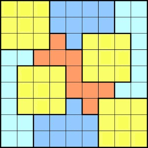
Figure 1: Our instance of Jigsaw problem.

6.2 [Q1] QuAcq2 in its basic setting

When QuAcq2 is used in its basic setting, we denote it by QuAcq2.basic. What we call the basic setting is when, in line 1 of Algorithm 1, QuAcq2 uses the function GenerateExample.basic described in Algorithm 4. GenerateExample.basic computes a complete assignment on $X$ satisfying the constraints in $L$ and violating at least one constraint from $B$. We build a network $C$ that contains the constraints from the network $L$ already learned (line 4), plus a reification of the constraints in $B$. A Boolean $b_{i}$ is introduced for each $c_{i}\in B$. This Boolean is forced to be true if and only if the constraint $c_{i}$ is satisfied (line 4). We then force the sum of $b_{i}$’s not to be equal to $|B|$ (line 4). Function $solve$ is called on $C$ (line 4) and returns a solution of $C$, or $\bot$ if no solution exists. Finally, the projection on $X$ of the solution is returned (line 4). The constraint solver inside $solve$ uses the dom/wdeg variable ordering heuristic [13] and a random value selection.

1 $C\leftarrow L$;

2 foreach $c_{i}\in B$ do  $C\leftarrow C\cup\{b_{i}\leftrightarrow c_{i}\}$;

3 $C\leftarrow C\cup\{\sum b_{i}\neq|B|\}$;

4 $e\leftarrow solve(C)$;

5 return $e[X]$;

Algorithm 4 $\texttt{Generate\-Example}.\texttt{basic}(X,B,L)$

Table 3: QuAcq2.basic. All results are averages of ten runs (time in seconds).

Instance	$|T|$	$|L|$	${\tt\#Q_{A}}$	${\tt\#Q_{C}}$	${\tt\overline{|Q|}}$/$|X|$	${\tt time_{A}}$	${\tt time_{C}}$	${\tt\overline{t}}$	${\tt t_{max}}$	${\tt\#C}$
Purdey	27	26.2	175.3	177.1	5.0/12	0.08	0.09	0.00	0.01	10
Zebra	64	61.1	555.6	555.8	8.1/25	2.54	2.54	0.00	1.50	10
Golomb	350	96.4	351.5	351.5	4.8/8	116.39	217.34	0.33	8.70	10
Random	122	122.0	1 082.2	1 092.0	20.8/50	2.08	85.94	0.08	83.80	7
RLFAP	125	98.5	1 103.6	–	–	43.35	–	–	$\tt TO$	0
Sudoku	810	775.7	6 849.9	–	–	214.16	–	–	$\tt TO$	0
Jigsaw	811	764.0	6 749.6	–	–	224.18	–	–	$\tt TO$	0
$\tt TO$ = 1 hour

Table 3 reports the results of running QuAcq2.basic on all our benchmark problems. The first observation we can make by looking at the table is that there are only four problems on which QuAcq2.basic has been able to converge in all of the ten runs (Purdey, Zebra, Golomb) or in some of them (Random). For Random, on which QuAcq2.basic converges 7 times out of 10, Table 3 reports the averages of these 7 runs.

We first focus our attention on these four problems: Purdey, Zebra, Golomb, and Random. Let us first compare the columns $|T|$ and $|L|$. On Purdey and Zebra, we observe that the size of $L$ is slightly smaller than the size of the target network $T$. This is due to a few constraints that are redundant wrt to some subsets of $T$. On Golomb, $|L|\ll|T|$ (96 and 350 respectively) because our target network with all quaternary constraints $|X_{i}-X_{j}|\neq|X_{k}-X_{l}|$ contains a lot of redundancies QuAcq2.basic detects convergence before learning them. Finally, as Random does not have any structure, it does not contain any redundant constraint, and $|L|=|T|$. The column ${\tt\overline{|Q|}}$/$|X|$ shows us that the queries asked by QuAcq2.basic are often much shorter than $|X|$. The average size ${\tt\overline{|Q|}}$ of queries varies from one third to one half of $|X|$. The the number of queries ${\tt\#Q_{C}}$ is two to seven times smaller than the size of the basis $B$. This means that each positive query leads to the removal of several constraints from $B$. Let us now compare the costs of finding the right network (columns ${\tt\#Q_{A}}$ and ${\tt time_{A}}$) and the costs of converging (columns ${\tt\#Q_{C}}$ and ${\tt time_{C}}$). This tells us a lot about the end of the learning process. On Purdey and Zebra, ${\tt\#Q_{A}}$ and ${\tt time_{A}}$ are similar to ${\tt\#Q_{C}}$ and ${\tt time_{C}}$ (respectively), which means that QuAcq2.basic learns constraints until the very end of the process. On Golomb, ${\tt\#Q_{A}}$ and ${\tt\#Q_{C}}$ are again similar, but ${\tt time_{C}}$ is much larger than ${\tt time_{A}}$. The reason is that after having learned all the constraints necessary to have a $L$ equivalent to $T$, GenerateExample.basic spends 100 seconds to show that $L\models B$, which proves convergence. On Random, we observe yet another behavior. As on Golomb, ${\tt time_{C}}$ is much larger than ${\tt time_{A}}$ (almost two orders of magnitude larger), but ${\tt\#Q_{C}}$ is also larger than ${\tt\#Q_{A}}$. The reason is that QuAcq2.basic has found a network $L$ equivalent to $T$ ten queries before the end and spends the end of the learning process generating complete queries that are positive and that allow QuAcq2.basic to remove useless constraints from $B$ and finally prove convergence. This last phenomenon is probably due to the sparseness of $T$ in Random. The columns ${\tt\overline{t}}$ and ${\tt t_{max}}$ tell us that most queries are very easy to generate (from milliseconds to one third of a second in average) and that most of the time is in fact consumed by generating the last positive queries. Random is an extreme case where the very last query consumes forty times the time needed for the whole process of learning $T$.

Let us now move our attention to the last three problems in Table 3, namely, RLFAP, Sudoku, and Jigsaw. On these problems, on each of the ten runs, QuAcq2.basic reaches the 1-hour cutoff on the time to generate a query. However we see that ${\tt\#Q_{A}}$ and ${\tt time_{A}}$, which represent the cost of learning a network equivalent to $T$ without having proved convergence, are reported in the table. For all the runs and all problems, QuAcq2.basic has found a network $L$ equivalent to $T$ before reaching the cutoff. This is the proof of convergence that leads QuAcq2.basic to the time-out. ${\tt\#Q_{A}}$ and ${\tt time_{A}}$ represent the cost of learning a network equivalent to $T$ but QuAcq2.basic does not know it is the target. Similarly to the first four problems, the number of queries required to learn a network equivalent to $T$ is significantly smaller than the size of $B$ (from three to eleven times smaller).

From this first experiment we conclude that QuAcq2.basic learns small constraint networks in a number of queries always significantly smaller than the size of the basis and generates queries in very short times. However, as soon as the size of the target network increases, the time to generate the last queries becomes prohibitive for an interactive learning process.

6.3 [Q2] Faster query generation

6.3.1 GenerateExample.cutoff: Generating (partial) queries with a time limit

The experiments in Section 6.2 have shown that QuAcq2.basic can be subject to excessive waiting time between two queries. This prevents its use in an interactive process where a human is in the loop. In this section we propose a new version of GenerateExample that fixes this weakness. We start from the observation that the example generated by GenerateExample in line 1 of Algorithm 1 does not need to be an assignment on $X$. Any partial assignment is satisfactory as long as it does not violate any constraint from $L$ and violates at least one constraint from $B$. We propose thus GenerateExample.cutoff, a new version of GenerateExample that quickly returns a partial assignment on a subset $Y$ of $X$ accepted by $L$ and violating at least one constraint from $B$. The main idea is to modify the function $solve$ so that it can be called with a cutoff.

Function $solve(C,S,obj,ub)$ takes as input a set $C$ of constraints to satisfy, a set $S$ of variables that must be included in the assignment, a parameter $obj$ to maximize, and an upper bound $ub$ on the time allocated. $solve$ returns a pair $(e_{Y},t)$ where $e_{Y}$ is an assignment on a set $Y$ of variables containing $S$, and $t$ is the time consumed by $solve$. If $solve$ proves that $C$ is inconsistent (that is, it found a set $Y$ containing $S$ for which every assignment on $Y$ either violates $C[Y]$ or leads to arc inconsistency on $C$), it returns the pair $(\bot,t)$ where $t$ is the time needed to prove that $C$ is inconsistent. If the allocated time $ub$ is not sufficient to find a satisfying assignment or prove an inconsistency, $solve$ returns the pair $(nil,ub)$. Otherwise, $solve$ returns a pair $(e_{Y},t)$ where $e_{Y}$ is an assignment accepted by $C$ and with highest value of $obj$ found during the allocated time $ub$, and $t$ is the time consumed. When $solve$ is called with $obj=nil$, there is nothing to maximize and the first satisfying assignment (on $S$) is returned. The function $solve$ uses the bdeg variable ordering heuristic [25]. bdeg selects the variable involved in a maximum number of constraints from $B$. By following bdeg, $solve$ tends to generate assignments that violate more constraints from $B$, so that in case of yes answer, the size of $B$ decreases faster.

1 $\texttt{time}\leftarrow 0$;

2

3foreach $c\in B$ do

4       $(e_{var(c)},t)\leftarrow solve(L\cup\{\neg c\},var(c),nil,+\infty)$;

5       $\texttt{time}\leftarrow\texttt{time}+t$;

6      

7      if $e_{var(c)}=\bot$ then

8             mark $c$ as redundant; $L\leftarrow L\cup\{c\}$; $B\leftarrow B\setminus\{c\}$;

9            

10       else

11             $(e^{\prime}_{Y},t^{\prime})\leftarrow solve(L\cup\{\neg c\},var(c),|Y|,\mathsf{cutoff}-\texttt{time})$;

12             $\texttt{time}\leftarrow\texttt{time}+t^{\prime}$;

13             if $e^{\prime}_{Y}=nil$ then return $e_{var(c)}$;

14             if $e^{\prime}_{Y}=\bot$ then

15                   mark $c$ as redundant; $L\leftarrow L\cup\{c\}$; $B\leftarrow B\setminus\{c\}$;

16                  

17             else return $e^{\prime}_{Y}$;

18            

19      

20remove all constraints marked as redundant from $L$;

21 return $\bot$;

Algorithm 5 $\texttt{Generate\-Example}.\texttt{cutoff}(X,B,L)$

Algorithm 5 describes GenerateExample.cutoff. GenerateExample.cutoff takes as input the set of variables $X$, a current basis of constraints $B$, a current learned network $L$ and a timeout parameter $\mathsf{cutoff}$. GenerateExample.cutoff iteratively picks a constraint $c$ from $B$ until a satisfying assignment is returned or $B$ is exhausted (line 5). The call to $solve$ in line 5 computes an assignment $e_{var(c)}$ on ${var(c)}$ violating $c$ and accepted by $L$. The time $t$ needed to compute $e_{var(c)}$ is added to the time counter (line 5). If $solve$ returns $e_{var(c)}=\bot$ (i.e., $L\cup\{\neg c\}$ is inconsistent), $c$ is marked as redundant because it is implied by $L$. $c$ is then removed from $B$ and added to $L$ (line 5). Adding $c$ to $L$ is required to avoid that QuAcq2 will later try to learn this constraint which is no longer in $B$. If $solve$ returns an assignment $e_{var(c)}$ different from $\bot$, GenerateExample.cutoff enters a second phase during which a second call to $solve$ will use the remaining amount of time, $\mathsf{cutoff}-time$, to compute an assignment $e^{\prime}_{Y}$ violating $c$ and accepted by $L$, whilst maximizing $|Y|$ (line 5). If no such assignment is found in the remaining time, $solve$ returns an $e^{\prime}_{Y}$ equal to $nil$ and GenerateExample.cutoff returns the $e_{var(c)}$ found by the first call to $solve$ (line 5). If $solve$ proved the inconsistency of $L\cup\{\neg c\}$ over a given scope $Y$ (i.e., $e^{\prime}_{Y}=\bot$), $c$ is marked as redundant, removed from $B$, and added to $L$ (line 5), exactly like line 5. GenerateExample.cutoff then goes back to line 5 to select a new constraint from $B$. Otherwise (i.e., $e^{\prime}_{Y}\notin\{nil,\bot\}$), GenerateExample.cutoff returns the assignment $e^{\prime}_{Y}$ with the largest size of $Y$ that has been found in the allocated time (line 5). Finally, if all constraints in $B$ have been processed without finding a suitable assignment (line 5), this means that all the constraints that were in $B$ were implied by $L$. The learning process has thus converged. We just need to remove all constraints marked as redundant from $L$ (line 5) and GenerateExample.cutoff returns $\bot$ (line 5). It is not necessary to remove the redundant constraints but it usually makes the learned network more compact and easier to understand.

6.3.2 Evaluation of GenerateExample.cutoff

We made the same experiments as in Section 6.2 but instead of using QuAcq2.basic, we used QuAcq2.cutoff, that is, QuAcq2 calling GenerateExample.cutoff. We have set the cutoff to one second so that the acquisition process remains comfortable in the case where the learner interacts with a human. Table 4 reports the results for the same measures as in Table 3.

Table 4: QuAcq2.cutoff with $\mathsf{cutoff}$ = 1 second.

Instance	$|T|$	$|L|$	${\tt\#Q_{A}}$	${\tt\#Q_{C}}$	${\tt\overline{|Q|}}$/$|X|$	${\tt time_{A}}$	${\tt time_{C}}$	${\tt\overline{t}}$	${\tt t_{max}}$	${\tt\#C}$
Purdey	27	26.3	172.3	179.1	5.3/12	0.09	0.20	0.00	0.03	10
Zebra	64	61.2	556.5	561.2	8.1/25	3.92	4.27	0.01	2.31	10
Golomb	350	98.0	377.2	377.2	4.2/8	135.32	138.06	0.36	8.47	10
Random	122	122.0	1 059.7	1 064.8	20.6/50	2.17	2.20	0.00	0.07	10
RLFAP	125	125.0	1 167.8	1 167.8	19.4/50	42.82	42.82	0.04	1.05	10
Sudoku	810	810.0	6 939.0	6 941.6	21.5/81	164.05	164.32	0.02	1.01	10
Jigsaw	811	811.0	6 874.5	6 880.2	21.0/81	225.40	231.04	0.03	1.01	10

The main information that we extract from Table 4 is that the use of GenerateExample.cutoff has a dramatic impact on the time consumption of generating queries. The cumulated generation time for all queries until convergence never exceeds five minutes on any run on any problem whereas QuAcq2.basic was reaching the one-hour cutoff for a query on all runs on three of the problems. Even on the problems where QuAcq2.basic was converging, QuAcq2.cutoff can show a significant speed up. For instance, on Random, QuAcq2.basic was taking a long time to prove that the learned network was equivalent to the target one (${\tt time_{C}}$ $\mathsf{g}$ ${\tt time_{A}}$). With QuAcq2.cutoff, ${\tt time_{C}}$ and ${\tt time_{A}}$ are almost equal and are close to the value of ${\tt time_{A}}$ of QuAcq2.basic.

We could have expected that the generation of shorter queries at the end of the learning process leads to an increase in the overall number of queries for QuAcq2.cutoff because shorter positive queries lead to fewer redundant constraints detected. But, when comparing ${\tt\#Q_{A}}$ and ${\tt\#Q_{C}}$ in Tables 3 and 4, we see that the increase is negligible. There is a -2% to +2% difference on most problems. The exceptions are Golomb and RLFAP, on which QuAcq2.cutoff exhibits an increase of 6% and 7% respectively. Similarly, ${\tt\overline{|Q|}}$/$|X|$ is essentially the same for QuAcq2.basic and QuAcq2.cutoff. As a last observation on Table 4, it can seem surprising that ${\tt t_{max}}$ is more than eight seconds on Golomb despite the cutoff of one second in GenerateExample.cutoff. This is because during the learning process, GenerateExample.cutoff repetitively finds redundant constraints without asking a question to the user (line 5 in Algorithm 5).

This experiment shows us that the introduction of a cutoff in the generation of examples completely solves the issue of extremely long waiting times at the end of the process. QuAcq2.cutoff learned all our benchmarks problems with extremely fast query generation. The only price to pay is a slight increase in number of queries in two of the problems.

6.4 [Q3] QuAcq2 with background knowledge

In practical applications, it is often the case that the user already knows some of the constraints of her problem. These constraints can be known because they are easy to express, or because they are implied by the structure of the problem, or because they have been learned by another tool. For instance, given a solution to a sudoku or to a jigsaw sudoku, ModelSeeker would be able to learn that all the cells in a row must take different values. We can also inherit constraints from a past/obsolete model that needs to be updated because some changes have occurred in the problem. For instance, if new workers have joined the company, we need to learn constraints on them, but the rest of the problem remains unchanged. This set of already known constraints will be called the background knowledge.

QuAcq2 can easily be adapted to handle the case of a background knowledge. In the following, a background knowledge will be a set $K$ of constraints, where $K$ is the part of the target problem that we already know, that is, $K\subseteq T$. Instead of calling QuAcq2 with an empty network $L$ and a basis $B$, QuAcq2 is called with $L$ initialized to $K$ and the basis initialized to $B\setminus\{K\cup\bar{K}\}$, where $\bar{K}=\{c\mid\neg c\in K\}$.

We performed a first experiment with Purdey, Zebra, Golomb, and Jigsaw. In Purdey, we assume that the user was able to express that if four different families buy four different items with four different paying means, then there is a clique of dis-equalities on the four variables representing families, a clique of dis-equalities on the variables representing items to buy, and also a clique on the variables representing paying means. Similarly, in Zebra, we assume that the user was able to express that if there are five people of five different nationalities, there is a clique of dis-equalities on the five variables representing nationalities. Idem on colors of houses, drinks, cigarettes and pets. In Golomb, we assume the user was able to express the symmetry breaking constraint $X_{i}<X_{j}$ for all pairs of marks $i,j,i<j$. Finally, in Jigsaw, we assume that the user ran ModelSeeker on the solutions of a few instances of these problems and learned that there is a clique of dis-equalities on all the rows and all the columns.

Table 5: QuAcq2.cutoff when the cliques of disequalities are already given in Purdey, Zebra, and Jigsaw, and the symmetry-breaking constraints in Golomb.

Instance	$|T|$	$|K|$	$|L|\setminus|K|$	${\tt\#Q_{A}}$	${\tt\#Q_{C}}$	${\tt\overline{|Q|}}$	${\tt time_{A}}$	${\tt time_{C}}$	${\tt\overline{t}}$	${\tt t_{max}}$
Purdey	27	18	9.0	70.8	81.5	5.6/12	0.05	0.24	0.00	0.03
Zebra	64	50	14.0	185.6	199.2	7.1/25	3.91	4.87	0.02	2.92
Golomb	350	28	70.0	246.5	246.5	5.1/8	132.10	139.51	0.53	6.00
Jigsaw	811	648	163.0	1 688.8	1 715.0	20.5/81	175.37	201.29	0.12	1.03

Table 5 reports the results when running QuAcq2.cutoff with an $L$ initialized to $K$ as described above for the four problems. The main observation is that the number of queries asked by QuAcq2.cutoff significantly decreases. This decrease in number of queries goes from a factor 1.5 for Golomb, where $|K|/|T|\approx 0.08$, 2.2 for Purdey, where $|K|/|T|\approx 0.67$, 2.8 for Zebra, where $|K|/|T|\approx 0.78$, to 4.0 for Jigsaw, where $|K|/|T|\approx 0.80$. This shows that the larger the number of constraints already known, the greater the decrease in number of queries. These are good news because the number of queries is a critical criterion when the user is a human. The second interesting information we learn from this experiment is that most of the other characteristics of QuAcq2.cutoff are essentially the same whatever QuAcq2.cutoff is provided with an initial background knowledge or not. The only exception is the average time to generate a query, ${\tt\overline{t}}$, that tends to increase in the presence of a background knowledge. This is not surprising because we know that this is when we are close to the end of the acquisition process —when $L$ is large— that query generation costs the most. But this increase only occurs because our queries are very fast to generate, faster than the cutoff of one second. If queries were becoming too long to generate, the cutoff would force shorter queries.

We performed a second experiment on Random, RLFAP, Sudoku, and Jigsaw, that are the problems on which QuAcq2.cutoff asks the more queries. Similarly to the previous experiment, we called QuAcq2.cutoff with a learned network $L$ partially filled with a background knowledge $K$ and a basis initialized to $B\setminus\{K\cup\bar{K}\}$. We varied the size of $K$ by randomly picking from 0% to 90% of the constraints in the target network.

Figure 2 reports the ratio ${\tt\#Q_{C}}$-w$K$/${\tt\#Q_{C}}$-wo$K$ of the number of queries that QuAcq2.cutoff requires to converge with a given $K$ on the number of queries required to converge without any $K$. These results show that when the size of $K$ increases, the number of queries decreases. On RLFAP, QuAcq2.cutoff drops from 1168 queries without $K$ to only 13 queries when $K$ contains 90% of the target network. Importantly, on all problems the decrease is strongly correlated to the amount of background knowledge provided (slope almost linear). This is very good news because this means that it always deserves to add more background knowledge.

Figure 2: ${\tt\#Q_{C}}$-w$K$/${\tt\#Q_{C}}$-wo$K$ for QuAcq2.cutoff when varying the size of $K$.

We do not report any result on QuAcq2.basic with background knowledge. Whatever the amount of background knowledge provided, QuAcq2.basic suffers from the same drawback as QuAcq2.basic without background knowledge: the last few queries are prohibitively expensive to generate. On RLFAP, Sudoku, and Jigsaw, QuAcq2.basic cannot converge on any run of any size of $K$ within the one-hour time limit on query generation time.

6.5 Discussion

These experiments tell us several important features of QuAcq2. These experiments show us that QuAcq2 can learn any kind of network, whatever all their constraints are organized with a specific structure (such as Sudoku), some of their constraints have a structure (Purdey, Zebra, Golomb, Jigsaw), or they have no structure at all (Random, RLFAP).

A second general observation is that QuAcq2 learns a network in a number of queries always significantly smaller than the size of the basis. This confirms that QuAcq2 is able to select the queries in a way that makes them very informative for the learning process. However, the experiment in Section 6.2 shows that when QuAcq2 is used in its basic version, the time to generate queries can be prohibitive, especially when interacting with a human. We indeed observe that when we are close to the end of the learning process, it can be extremely time consuming to generate a complete example at the start of each loop of acquisition of QuAcq2.

The experiment in Section 6.3.2 shows that a simple adaptation of the way examples are generated (see function GenerateExample.1 in Section 6.3.1), allow us to monitor the CPU time needed to generate an example with a cutoff. In the experiment we see that a cutoff of one second leads to a very smooth interaction between the learner and the user. It is important to bear in mind that even with a cutoff, QuAcq2 ensures the property of convergence.

All experiments in Sections 6.2 and 6.3.2 were performed in the scenario where we do not have any background knowledge about the problem. In these experiments, QuAcq2 is always initialized with an empty learned network $L$. As a result, the number of queries necessary on some of the benchmark problems can seem unrealistic for a real use, especially in the presence of a human user. But it is often the case that the user is able to express some of the constraints of the problem, or that an initial subset of the constraints can be learned with a tool such as ModelSeeker or Arnold. Such tools are able to learn constraints with very few examples when these constraints follow some specific structure. In such scenarios, QuAcq2 can be used as a complement that will learn the missing constraints, that is, the constraint that cannot be captured in a specific structure recognized by these tools. Our experiment in Section 6.4 shows that QuAcq2 is extremely good when it is provided with a background knowledge in the form of a set of constraints. The larger the set of constraints given as a background knowledge, the fewer queries needed to learn the network.

7 Conclusion

We have proposed QuAcq2, an algorithm that learns constraint networks by asking the user to classify partial assignments as positive or negative. Each time it receives a negative example, the algorithm converges on a constraint of the target network in a logarithmic number of queries. Asking the user to classify partial assignments allows QuAcq2 to converge on the target constraint network in a polynomial number of queries (as opposed to the exponential number of queries required when learning with membership queries only). We have shown that QuAcq2 is optimal on certain constraint languages and that it is close to optimal (up to $\log n$ worse) on others. Furthermore, as opposed to other techniques, the user does not need to provide positive examples to learn the target network. This can be very useful when the problem has never been solved before. Our experiments show that QuAcq2 in its basic version can be time consuming but they also show that QuAcq2 can be parameterized with a cutoff on the waiting time that allows it to generate queries quickly. These experiments also show that QuAcq2 can learn any kind of network, whatever its constraints follow a specific structure (such as matrices) or not. More, we observed that QuAcq2 behaves very well in the presence of a background knowledge. The larger the background knowledge, the fewer the queries required to converge on the target network. This last feature makes QuAcq2 a perfect candidate to learn missing constraints in a partially filled constraint model. As a last comment, we should bear in mind that all the improvements of QuAcq1 already published in the literature (for instance [26, 6, 15, 1, 25]), can be used with QuAcq2.

References

- [1] H.A. Addi, C. Bessiere, R. Ezzahir, and N. Lazaar. Time-bounded query generator for constraint acquisition. In Proceedings of the 15th International Conference on Integration of Constraint Programming, Artificial Intelligence, and Operations Research (CPAIOR 2018), pages 1–17, Delft, The Netherlands, 2018. Springer.
- [2] D. Angluin. Queries and concept learning. Machine Learning, 2(4):319–342, 1987.
- [3] D. Angluin, M. Frazier, and L. Pitt. Learning conjunctions of horn clauses. Mach. Learn., 9:147–164, 1992.
- [4] N. Beldiceanu, M. Carlsson, and J.X. Rampon. Global constraint catalog. Technical Report T2005:08, Swedish Institute of Computer Science, Kista, Sweden, May 2005.
- [5] N. Beldiceanu and H. Simonis. A model seeker: Extracting global constraint models from positive examples. In Proceedings of the Seventeenth International Conference on Principles and Practice of Constraint Programming (CP’12), pages 141–157, Quebec City, Canada, 2012. Springer.
- [6] C. Bessiere, R. Coletta, A. Daoudi, N. Lazaar, Y. Mechqrane, and E.H. Bouyakhf. Boosting constraint acquisition via generalization queries. In Proceedings of the 21st European Conference on Artificial Intelligence, pages 99–104, Prague, Czech Republic, 2014. IOS Press.
- [7] C. Bessiere, R. Coletta, E. Freuder, and B. O’Sullivan. Leveraging the learning power of examples in automated constraint acquisition. In Proceedings of the Tenth International Conference on Principles and Practice of Constraint Programming (CP’04), pages 123–137, Toronto, Canada, 2004. Springer.
- [8] C. Bessiere, R. Coletta, E. Hebrard, G. Katsirelos, N. Lazaar, N. Narodytska, C.-G. Quimper, and T. Walsh. Constraint acquisition via partial queries. In Proceedings of the 23rd International Joint Conference on Artificial Intelligence, pages 475–481, Beijing, China, 2013.
- [9] C. Bessiere, R. Coletta, F. Koriche, and B. O’Sullivan. A SAT-based version space algorithm for acquiring constraint satisfaction problems. In Proceedings of the European Conference on Machine Learning (ECML’05), pages 23–34, Porto, Portugal, 2005. Springer.
- [10] C. Bessiere, R. Coletta, B O’Sullivan, and M. Paulin. Query-driven constraint acquisition. In Proceedings of the Twentieth International Joint Conference on Artificial Intelligence (IJCAI’07), pages 44–49, Hyderabad, India, 2007.
- [11] C. Bessiere and F. Koriche. Non learnability of constraint networks with membership queries. Technical report, Coconut, Montpellier, France, February 2012.
- [12] C. Bessiere, F. Koriche, N. Lazaar, and B. O’Sullivan. Constraint acquisition. Artif. Intell., 244:315–342, 2017.
- [13] F. Boussemart, F. Hemery, C. Lecoutre, and L. Sais. Boosting systematic search by weighting constraints. In Proceedings of the Sixteenth European Conference on Artificial Intelligence (ECAI’04), pages 146–150, Valencia, Spain, 2004.
- [14] B. Cabon, S. de Givry, L. Lobjois, T. Schiex, and J.P. Warners. Radio link frequency assignment. Constraints, 4(1):79–89, 1999.
- [15] A. Daoudi, Y. Mechqrane, C. Bessiere, N. Lazaar, and E.H. Bouyakhf. Constraint acquisition using recommendation queries. In Proceedings of the Twenty-Fifth International Joint Conference on Artificial Intelligence (IJCAI’16), pages 720–726, New York City, NY, 2016.
- [16] N.G. De Bruijn. Asymptotic Methods in Analysis. Dover Books on Mathematics. Dover Publications, 1970.
- [17] E.C. Freuder and R.J. Wallace. Suggestion strategies for constraint-based matchmaker agents. In Michael J. Maher and Jean-Francois Puget, editors, Proceedings of the 4th International Conference on Principles and Practice of Constraint Programming (CP98), pages 192–204, Pisa, Italy, 1998. Springer.
- [18] I.P. Gent and T. Walsh. Csplib: a benchmark library for constraints. http://www.csplib.org/, 1999.
- [19] U. Junker. Quickxplain: Preferred explanations and relaxations for over-constrained problems. In Proceedings of the Nineteenth National Conference on Artificial Intelligence (AAAI’04), pages 167–172, San Jose CA, 2004.
- [20] M. Kumar, S. Teso, and L. De Raedt. Acquiring integer programs from data. In Proceedings of the Twenty-Eighth International Joint Conference on Artificial Intelligence (IJCAI 2019), pages 1130–1136, Macao, China, 2019. ijcai.org.
- [21] A. Lallouet, M. Lopez, L. Martin, and C. Vrain. On learning constraint problems. In Proceedings of the 22nd IEEE International Conference on Tools for Artificial Intelligence (IEEE-ICTAI’10), pages 45–52, Arras, France, 2010.
- [22] J. Mason. Purdey’s general store. Dell Magazine, 54:10–10, April 1997.
- [23] M. Paulin, C. Bessiere, and J. Sallantin. Automatic design of robot behaviors through constraint network acquisition. In Proceedings of the 20th IEEE International Conference on Tools for Artificial Intelligence (IEEE-ICTAI’08), pages 275–282, Dayton OH, 2008.
- [24] L. De Raedt, A. Passerini, and S. Teso. Learning constraints from examples. In Proceedings of the Thirty-Second AAAI Conference on Artificial Intelligence (AAAI-18), pages 7965–7970, New Orleans, Louisiana, USA, 2018. AAAI Press.
- [25] D.C. Tsouros, K. Stergiou, and C. Bessiere. Structure-driven multiple constraint acquisition. In Proceedings of the 25th International Conference on Principles and Practice of Constraint Programming (CP 2019), pages 709–725, Stamford, CT, 2019. Springer.
- [26] D.C. Tsouros, K. Stergiou, and P.G. Sarigiannidis. Efficient methods for constraint acquisition. In John N. Hooker, editor, Proceedings of the 24th International Conference Principles and Practice of Constraint Programming (CP 2018), pages 373–388, Lille, France, 2018. Springer.