Graph Profiling for Vertex Cover:
Targeted Reductions in a Branch and Reduce Solver

Akiba and Iwata [TCS, 2016] demonstrated that a branch and reduce (B&R) solver for the vertex cover problem can compete favorably with integer linear programming solvers (e.g., CPLEX). Given a well-engineered B&R solver taking a reduction routine configuration as input, our research question is are there graph characteristics that determine which reductions will be most effective? Not only is the answer affirmative, but the relevant characteristics are easy to identify and compute.

In order to explore our ideas rigorously, we provide an enhanced implementation of the Akiba-Iwata solver so that it can (a) be configured with any subset of reductions and any applicable lower bounds; (b) print statistics such as time taken and number of vertices reduced by each reduction type; and (c) print trace information with additional details.

Based on extensive experiments with both benchmark and random instances we demonstrate that (i) doing more reductions does not necessarily lead to better runtimes (in fact, sometimes the best strategy is to use no reductions at all); (ii) in most cases, the subset of reductions leading to the best (or nearly the best) runtime can be predicted based on measurable characteristics of a graph, such as density of the graph and degree distribution; and (iii) the exceptions have structural characteristics that may be known in advance; examples include large sparse graphs, geometric graphs, and planar graphs.

Our primary contributions are

1. A thorough examination reduction routine performance in the context of graph characteristics.

2. Three primary hypotheses suggesting simple suites of reductions as the most efficient options.

3. Experiments with a large corpus of data to validate our hypotheses.

4. Measures that quantify a problem instance on two key dimensions to make our hypotheses concrete.

5. An enhanced open-source version of the Akiba-Iwata solver that enables our investigations and creates opportunities for future exploration.

Our main objective is to provide guidance to a user so that, faced with a given problem instance or set of instances, they may most effectively use the available reductions. Ultimately these efforts can lead to an automated process.

Categories and Subject Descriptors: G.2.2 [Discrete Mathematics]: Graph Theory – Graph Algorithms.

General Terms: Algorithms, Experimentation, Graphs, Performance.

Additional Key Words and Phrases: vertex cover, branch and reduce, dominance, folding.

1 Introduction

Originally one of Karp’s 21 NP-complete problems [21], Vertex Cover has a rich history in combinatorial optimization. While there are simple 2-approximation algorithms, the problem cannot be approximated below 1.36 [9], or below 2 when assuming the Unique Games Conjecture [22]. When solving exactly, Vertex Cover is fixed-parameter tractable in both the natural parameter (solution size) and also in structural graph properties such as treewidth [8]. Such exact solutions may be of interest in their own right [1, 27] or as a structural property utilized by an algorithm [10]. Additionally, Vertex Cover relates to several other optimization problems such as Independent Set, Maximum Clique, and Odd Cycle Transversal [2]. In some cases, reformulating these optimization problems and solving them with a Vertex Cover solver leads to faster algorithms [23].

In recent years researchers have developed vertex cover solvers scalable to large data. Minimum vertex cover (minVC) is easily converted to an Integer Linear Programming (ILP) instance, enabling the use of industrial-quality solvers such as CPLEX and Gurobi. Akiba and Iwata [2] showed that a branch-and-reduce (B&R) framework populated with several reduction routines, lower bound estimators, and branching rules could compete with both CPLEX and a Maximum Clique solver on social-network–sized datasets. In this paper we report how this B&R solver can be tuned for faster performance based on the provided instance. Specifically, we study how the choice of reduction configuration affects total performance.

In order to carry out these explorations, we provide an enhanced version of the Akiba-Iwata solver (VCS+) where (a) any subset of the provided reductions and lower bound methods can be selected; and (b) the output includes detailed statistics on the number of vertices reduced and the runtime spent for each reduction. Statistics related to the effectiveness of verious lower bounds are also provided. In our analysis we find that

• The set of reductions chosen for a particular problem instance matters, sometimes a great deal.

• Easily computed characteristics of a problem instance, based on concrete measures we define, can pinpoint the set of reductions that are likely to be most effective.

• In some cases, structural properties of the instance, such as whether it is planar, based on geometry, or simply very large and sparse, are the primary factor influencing the most efficient set of reductions.

To make the relationships between graph characteristics and performance of reductions more precise, we propose and experimentally validate five hypotheses. Outlined here, these are described and quantified in Section 5.

1. If the graph has low degree variation and density is large, the most promising option is to do no reductions at all.

2. If degree variation and density are large, the dominance reduction is effective.

3. Simple reductions, such as degree-1 and fold-2, are sufficient for most sparse graphs.

4. The effectiveness of the LP reduction is related to how close the graph is to being bipartite.

5. Sparse graphs with low degree variation are much harder to solve using B&R than others with the same number of vertices.

Our preliminary experiments involved over 40,000 trials on roughly 10,000 instances. The results reported here focus on a carefully selected set of roughly one thousand instances, with ’interesting’ runtimes, and at least six trials (using a different set of reductions for each trial) per instance.

The remainder of the paper is organized as follows. Section 2 provides definitions and outlines the concepts relevant to VCSolver; Section 3 motivates our study and distinguishes our experimental approach from that of Akiba and Iwata; Section 4 lists the problem instances in our corpus; Section 5 presents our main experimental results; Section 6 discusses special cases; and Section 7 summarizes our findings and suggests future work.

Appendix A outlines the B&R algorithm implemented by VCSolver; Appendix B shows the options and statistics provided by VCS+. Appendices C and D describe problem instances from other sources in detail; Appendix E describes the exceptions to the main hypotheses; and Appendix F has detailed tables that complement the figures in the main text.

Code and scripts for VCS+ are available at https://github.com/mfms-ncsu/VC-BR and a CPLEX driver at https://github.com/mfms-ncsu/CPX-ILP.

2 Background and Motivation

A graph $G=(V,E)$ has a vertex set $V$ and edge set $E\subseteq V\times V$. In this paper we assume that all graphs are simple and undirected. When clear from context, we denote $n=|V|$ and $m=|E|$. The neighborhood of $v$, set of adjacent vertices, is denoted $\mathrm{N}(v)$. If $v$ is included we use $\mathrm{N}[v]$.

A vertex cover of $G$ is a set of vertices $S\subseteq V$ such that $G\setminus S$ is edgeless. Formulated as an optimization problem, the objective of Vertex Cover is to find a minimum sized vertex cover. We refer to this as the minVC problem. A minVC instance can be converted into an Integer Linear Programming (ILP) instance by minimizing $\sum_{v\in V}x_{v}$ subject to $x_{u}+x_{v}\geq 1$ for each edge $uv$, and $x_{v}\in\{0,1\}$ for each vertex $v$. In other words, minimize the number of vertices in the cover, such that every edge is covered and each vertex is either in the cover or not. We implicitly use this conversion when solving minVC instances with CPLEX.

A related problem is Odd Cycle Transversal (OCT), the problem of computing a minimum set of vertices whose removal renders a graph odd cycle-free. Using a canonical transformation [2], an OCT instance can be transformed into a minVC instance with only constant blowup; in fact, there is precedent to think that OCT instances are best solved with minVC solvers [23].

In the remainder of this section we overview branching techniques such as branch-and-bound and branch-and-reduce, summarize the reduction rules provided in [2], and provide motivation for the current study.

2.1 Branch-and-reduce

Similar to branch-and-bound, the branch-and-reduce (B&R) paradigm iterates between branching, checking bounds, and running an ensemble of reduction routines to simplify the problem instance. A graph instance is reduced until the reductions no longer apply, then two branches are created (by choosing a vertex and either including it in the cover or excluding it), and each resulting sub-instance is reduced. At each step the partial solution and a lower bound on the current instance is compared against an upper bound, allowing the algorithm to quit a branch early if the lower bound is greater than or equal to the known upper bound.

Unlike preprocessing routines, only run once at the beginning of execution, the reduction routines are executed throughout the course of the full algorithm. Whereas ineffective preprocessing routines will incur wasted time for the initial instance only, ineffective reduction routines could waste time at a potentially exponential number of subinstances. Therefore it is of interest to identify which reduction routines will prove effective on the structures and substructures found over the full course of an execution.

Appendix A gives details of the general branch and reduce algorithm and Iwata’s implementation, VCSolver. Our enhanced version, VCS+, makes no changes beyond enabling an unconstrained choice of reductions and lower bounds. In addition, VCS+ outputs the actual solution obtained (as a bit vector), to allow verification and potential post-processing (when the solution is not optimal); and it outputs a large variety of statistics relevant to our study – see Appendix B.

2.2 Lower Bounds

The three nontrivial lower bounds in VCSolver are

• clique. If $C$ is a $k$-clique, then any vertex cover must include at least $k-1$ vertices of $C$. VCSolver employs a simple greedy strategy that collects vertices into cliques, largest first.

• LP. The linear programming relaxation of the ILP for minVC is a lower bound. This bound is applied when an LP reduction, see below, is done.

• cycle. If $C$ is a cycle with $k$ vertices, any vertex cover must include at least $\lceil k/2\rceil$ vertices of $C$. VCSolver applies the cycle lower bound only if an LP reduction has taken place and information about odd cycles is readily available.

Options provided by VCSolver are: $-l0$ (trivial lower bound only), $-l1$ (clique lower bound), $-l2$ (LP lower bound), $-l3$ (LP and cycle lower bounds), $-l4$ (all lower bounds).

2.3 Reduction rules

The reduction rules used in VCSolver are as follows. We refer the reader to Akiba and Iwata [2], Xiao and Nagamochi [28, 29] and Ho [17] for more details and proofs.

• degree-1. A degree-one vertex can be removed and its neighbor added to the cover.

• dominance. If $vw$ is an edge and $\mathrm{N}[v]\subseteq\mathrm{N}[w]$, then $w$ dominates $v$ and we can add $w$ to the cover.

• fold-2. If $\mathit{deg}(v)=2$ and its neighbors $u$ and $w$ are not adjacent, then we contract $u,v,w$ into a new vertex $z$ to form $G^{\prime}$; if $C^{\prime}$, a minimum cover of $G^{\prime}$, includes $z$ then $C^{\prime}-z\cup\{u,w\}$ is a minimum cover of $G$; otherwise $C^{\prime}\cup v$ is a minimum cover.

• twin. If $\mathrm{N}(v)=\mathrm{N}(w)$ and $\mathit{deg}(v)=\mathit{deg}(w)=3$ then $v$ and $w$ are twins; we contract $\mathrm{N}(v)$ into a single vertex $z$ to form $G^{\prime}$; if $C^{\prime}$, a minimum cover of $G^{\prime}$, contains $z$, then $C^{\prime}-z\cup\mathrm{N}(v)$ is a minimum cover of $G$; otherwise $C^{\prime}\cup v$ is.

  The fold-2 and twin reductions are special cases of a $k$-independent-set reduction – see [28, 29].

• LP. If $S$ is a solution to the LP-relaxation of the ILP for minVC, then there exists a minimum vertex cover that includes every vertex $v$ with $x_{v}=1$ and excludes every $v$ with $x_{v}=0$. Iwata et al. [18] give an algorithm that minimizes the number of variables with half-integer values.

• unconfined. [28] A vertex is unconfined if the following algorithm returns true.

  1. $S=\{v\}$.

  2. Find $u\in N(S)$ with $|N(u)\cap S|=1$ and having minimum value of $|N(u)\setminus N[S]|$.

  3. If no such $u$ exists or $|N(u)\setminus N[S]|>1$, then return false.

  4. If $N(u)\setminus N[S]=\emptyset$, then return true.

  5. Otherwise, $S=S\cup(N(u)\setminus N[S])$ and start again from step 2.

  Unconfined reductions generalize dominance – if the algorithm returns true during step 4 in the first iteration, then $v$ dominates $u$.

• funnel. If, for some $w\in\mathrm{N}(v)$, $\mathrm{N}[v]-w$ is a clique, we create $G^{\prime}$ by removing $v$, $w$, and $\mathrm{N}(v)\cap\mathrm{N}(w)$, and adding an edge $st$ between each $s\in\mathrm{N}(v)\setminus\mathrm{N}[w]$ and each $t\in\mathrm{N}(w)\setminus\mathrm{N}[v]$. Let $C^{\prime}$ be a minVC of $G^{\prime}$. If $\mathrm{N}(v)\setminus\mathrm{N}(w)\subseteq C^{\prime}$ then $C=C^{\prime}\cup w\cup(\mathrm{N}(v)\cap\mathrm{N}(w))$ is a minimum cover of $G$; otherwise $\mathrm{N}(w)\setminus\mathrm{N}(v)\subseteq C^{\prime}$ and $C=C^{\prime}\cup v\cup(\mathrm{N}(v)\cap\mathrm{N}(w))$ form a minimum cover of $G$.

• desk. If $v_{1},v_{2},v_{3},v_{4}$ is a chordless four-cycle, $\mathit{deg}(v_{i})\geq 3$ for $i=1,\ldots,4$, and $\mathrm{N}(v_{1},v_{3})\cap\mathrm{N}(v_{2},v_{4})=\emptyset$, then create $G^{\prime}$ by removing $v_{1},v_{2},v_{3},v_{4}$ and adding an edge between each $s\in\mathrm{N}(v_{1},v_{3})$ and each $t\in\mathrm{N}(v_{2},v_{4})$. Let $C^{\prime}$ by a minimum cover of $G^{\prime}$. If $\mathrm{N}(v_{1},v_{3})\subseteq C^{\prime}$ then $C=C^{\prime}\cup\{v_{2},v_{4}\}$ is a minimum cover of $G$; else $\mathrm{N}(v_{2},v_{4})\subseteq C^{\prime}$ and $C=C^{\prime}\cup\{v_{1},v_{3}\}$ is a minimum cover of $G$.

The funnel and desk reductions are special cases of alternative reductions – see [28].

2.4 Related work

Some recent research addresses the relationship between graph characteristics and vertex cover complexity. For example, Bläsius et al. [6] show that minVC on hyperbolic random graphs can be solved in polynomial time. These graphs model the degree distribution and clustering of many real-world graphs. Though we have not experimented specifically with these graphs, we note that VCS+, with appropriate choice of reductions, is efficient on graphs with similar characteristics. Recent work also addresses use of various combinations of reductions to obtain algorithms that are efficient in practice. Hespe et al. [16] make effective use of parallelism. Chang et al. [7] use reductions in a linear-time heuristic that generates high quality solutions in practice (for the related maximum independent set problem). Other researchers have demonstrated that the combination of degree-1 and fold-2, used in preprocessing, is effective for many real-world instances – see, e.g., Strash [26]. We have found that this combination is effective when used throughout execution for most benchmark and randomly generated instances, including ones from the recent PACE-2019 vertex cover challenge [24].

3 Reduction Configurations

One of our main contributions is the analysis of individual reductions and combinations of reductions, particularly those not offered by the original VCSolver.

The reduction options offered by VCSolver are limited and cumulative, such that r0 $\subseteq$ r1 $\subseteq$ r2 $\subseteq$ r3. The r0 level includes degree-1, dominance, and fold-2; level r1 adds LP; level r2 adds twin, desk, unconfined, and funnel; and level r3 adds packing. The degree-1, fold-2, twin, desk, and packing reductions all take linear time, while LP is linear after an initial $O(m\sqrt{n})$ to set up an auxiliary graph and compute a matching. Dominance and unconfined are $\Theta(d^{2}n)$ and $\Theta(d^{3}n)$, respectively, where $d$ is the maximum degree.

Based on a limited set of problem instances, Akiba and Iwata concluded that using all reductions and all lower bounds (their -r3 -l4 options) is (almost) always best. We discovered, however, that for many of the problem instances from the full benchmark corpus, the fastest runtime was achieved without using any reductions at all and using only the lower bound based on a clique cover. For these instances at least, we show, effectively, that VCSolver is a well-engineered branch-and-bound solver.

Table 1 is a stark illustration. These particular instances were selected from the thousands in our experiments based purely on runtime, with the following characteristics: (i) runtime differences are significant, often differing by an order of magnitude; and (ii) CPLEX is not a good option (runtime yet another order of magnitude worse). One characteristic they share is that they are extremely dense; so it is no surprise that reductions designed for sparse instances are ineffective, whereas a clique lower bound is. In our experiments we explore a middle ground between choosing no reductions and choosing all of them.

Table 1: Selected instances where the best runtimes are achieved with no reductions.

Instance	None	-r2 -l4	-r3 -l4	CPLEX
san1000	30.93	305.46	762.71	$>900$
DSJC1000.9	27.90	232.12	699.34	$>900$
p_hat700-1	12.47	97.47	218.92	$>900$
c-fat500-1	2.26	7.29	7.32	71.92

(a) runtimes: None means clique lower bound only; the other columns represent VCSolver options.

Instance	vertices	min	avg	max
san1000	1,000	449	498.0	554
DSJC1000.9	1,000	870	898.9	924
p_hat700-1	700	413	524.7	624
c-fat500-1	500	479	481.2	482

(b) degree statistics

Table 2: The median effectiveness and efficiency of various reductions.

reduction	$\mu$sec/vertex		% reduced
	med	geo	med	geo
fold2	1.2	1.3	71.2	62.4
unconf.	24.6	21.6	9.1	9.9
lp	51.5	70.0	4.5	3.5
pack.	59.4	69.4	3.5	2.4
deg1	6.1	8.1	2.8	1.9
fun.	81.8	136.3	2.0	1.2
desk	108.5	129.7	0.8	0.8
twin	96.3	117.2	0.5	0.5
dom.	236.8	331.7	0.3	0.3

Efficiency, for a reduction type, is measured as the time spent per vertex reduced, in microseconds. Effectiveness is percentage of vertices reduced with respect to number of vertices reduced overall. Measurements are based on the -r3 -l4 options, which include all reductions and all lower bounds. Given the large variation among problem instances in the corpus (goldilocks instances), we report both the medians and the geometric means. The reductions are sorted by decreasing frequency (last two columns).

To that end, we analyzed the effectiveness and efficiency of various reductions over our corpus – see Table 2. A disadvantage of VCSolver, already noted, is that the choice of reductions is limited. In particular, the smallest subset includes dominance, overall the most time-consuming and least effective. To emphasize the flexibility of VCS+, we use the term reduction configuration (or simply config) to refer to a set of reductions and lower bounds performed by a trial of VCS+. In preliminary experiments (before we compiled the results in Table 2) we discovered that, on most instances where reductions paid off at all, the config that includes most of the linear time ones, Cheap (degree-1, fold-2, desk, twin), gave the best runtimes.

Table 3: Configurations used in our experiments

Name	Reductions	Lower Bounds
Used in preliminary experiments
None		clique
Deg1	deg1	clique
DD	deg1 dom	clique
Cheap	deg1 fold2 desk twin	clique
All	deg1 dom fold2 LP unconfined funnel desk twin	clique lp
Used in comprehensive experiments
Fold2	fold2	clique
DF2	deg1 fold2	clique
r0_l1	deg1 dom fold2	clique
r0_l1+U	deg1 dom fold2 unconfined	clique
r2_l4	deg1 dom fold2 LP unconfined twin funnel desk	clique lp cycle
r3_l4	deg1 dom fold2 LP unconfined twin funnel desk packing	clique lp cycle
Used in experiments with large sparse graphs
Cheap+U	deg1 fold2 unconfined desk twin	clique
Cheap+LP	deg1 fold2 LP desk twin	clique lp
Cheap+LPU	deg1 fold2 LP unconfined desk twin	clique lp
DF2+U	deg1 fold2 unconfined	clique
DF2+LP	deg1 fold2 LP	clique lp
DF2+LPU	deg1 fold2 LP unconfined	clique lp

Table 3 lists the important configs used in our trials. We used the first group in preliminary experiments on most instances to establish the effectiveness of key reductions. In later experiments, focused on goldilocks instances, ones where at least one of the initial configs took $>2$ seconds and at least one took $<600$, we added Fold2 and DF2 (the two most efficient reductions). For comparison, we also added configs offered by the original VCSolver: r0_l1, r2_l4, and r3_l4. Finally, we added r0_l1+U, the -r0 -l1 option of VCSolver with unconfined added (the most frequent after fold-2). So five additional configs.

When doing experiments with special cases – large sparse, geometric, and planar graphs, we added unconfined and/or LP to the Cheap config and to the DF2 config, as suggested by Table 2.

Focusing on runtime, a reduction configuration is said to be competitive for a given problem instance $x$ if its runtime for $x$ is within a factor of 2 (binary order of magnitude) of the minimum. The definition is robust in the sense that it appears to be invariant for trials on radically different machine architectures (cache size being the major factor: 512 KB, 4 MB, 12 MB, 20 MB, or 30 MB) and multiple trials with permuted inputs for the same instance.

A collection $\mathcal{C}$ of reduction configurations is globally competitive over a set of problem instances $\mathcal{I}$ if, for every instance $x\in\mathcal{I}$, at least one reduction set in $\mathcal{C}$ is competitive for $x$. In our preliminary experiments the collection $\{\textsf{None},\textsf{Cheap},\textsf{All}\}$ was globally competitive for all instances. In the more comprehensive experiments on goldilocks instances the collection $\{\textsf{None},\textsf{DF2},\textsf{r0\_l1}\}$ was globally competitive for all but a few exceptions.

4 Problem Instances

Before introducing problem instances we define the measures that characterize them and the resulting two-dimensional landscape. We take special care to introduce random instances that populate as much of the landscape as possible.

4.1 Instance measures

The most obvious of measure is density – many of the reductions are designed specifically for sparse graphs while the densest graphs have large cliques, making the clique lower bound effective without reductions. We use normalized average degree (nad), a hybrid of traditional density and actual average degree. Specifically, if average degree is $>20$, we normalize it using a factor of $200/n$ (most of our randomly generated graphs have roughly 200 vertices), so a complete graph has $\textsl{nad}=199$. When $\leq 20$ we use the actual average degree; the threshold is arbitrary, but, at the low end, reductions and branching lead to trivial subinstances at a rate determined by actual average degree.

The degree spread, or simply spread, captures the fact that the when $\mathit{deg}(v)$ is small and $v$ has high degree neighbors, max-degree branching will quickly make $v$ eligible for degree-1 or fold-2 reductions. We define spread to be $t/b$, where $t$ is the degree at the 95-th percentile and $b$ at the 5-th. This is an arbitrary choice, but the landscape does not change much if we use, for example, the 90-th and the 10-th. In the extreme, when both spread and nad are high, the probability of dominance becomes non-negligible: $\frac{k!}{(k-j)!}\cdot\frac{(n-k)!}{n!}$ for two vertices of degree $k$ and $j\ll k$.

To effectively visualize trials on a corpus of hundreds of graphs we use a landscape plot (log-log) with spread on the x-axis and nad on the y-axis. Fig. 1 shows our randomly generated instances on the landscape.

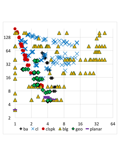
Randomly generated instances of various flavors: Barabasi-Albert, two types of Chung-Lu (uniform/normal distribution and clspk is ’spiked’ – a few vertices at extreme degrees and almost all in the middle), geometric, planar, and blg. The blg (bucket list generator) produces connected graphs and gives full control of min, max, and average degree, thus allowing fuller coverage of the landscape.

Figure 1: The landscape of random instances.

4.2 Random instances

Our random instances fall into several categories. The first of these, blg, is of our own design, keeping the landscape in mind. The rest are based on standard techniques.

blg. The generator for these, bucket list generator (blg) was created specifically for our preliminary experiments to saturate the landscape. The blg takes as input the number of vertices, average degree, and a $dv$ parameter. The generator guarantees connectivity by initially creating a random spanning tree; then edges are added until the average degree is achieved.

Vertices are maintained in ‘buckets’ based on their degree. The parameter $dv$ determines the choice of endpoints for each edge: $dv=0$ means lowest degree vertices are chosen – this leads to regular (or nearly regular) graphs; if $dv=1$, endpoints are chosen uniform randomly; if $dv<1$ bias is toward endpoints of low degree, if $dv>1$ then bias is toward those of high degree – this leads to degree distributions that are approximately normal or approximately exponential, respectively.

In addition to the mandatory parameters, the generator has optional parameters to control (as much as possible) $d_{\mathrm{min}}$ and $d_{\mathrm{max}}$. Vertices whose degree is less than $d_{\mathrm{min}}$ are chosen unconditionally, while vertices with degree greater than $d_{\mathrm{max}}$ are no longer considered.

Most of our blg graphs have 200 vertices. In some cases, where this led to instances that were too easy or too hard, we generated corresponding ones with 250 or 150 vertices, respectively. Naming convention is blg-$n$_$a$_$dv$_$m$d$M$, where $n$ is the number of vertices, $a$ is the average degree, and $m$ and $M$ are the desired minimum and maximum degree, respectively.

ba. (Barabasi-Albert) We used the preferential attachment generator provided by the python networkx package, function barabasi_albert_graph. The only parameters are number of vertices and number of edges to be added by each new vertex. These graphs are connected. In our corpus most of the ba graphs have 256 vertices, but when these turned out to be too easy, we added ones with 512 or 999 vertices. Number of attachment edges ranged from 8 to 90. Naming convention is ba_$n$_$k$_$s$, where $n$, $k$, and $s$ are number of vertices, number of edges to be added, and the random seed, respectively.

cl and clspk. (Chung-Lu) Here we used the expected_degree_graph function from the networkx package. This requires a complete list of vertex degrees and the result is at best an approximation. Our cl graphs start with a uniform distribution of degrees from a specified min to a specified max. The result is closer to a normal distribution. Our clspk graphs start with one min and one max degree vertex and put other degrees somewhere in between. The result is a normal distribution with low standard deviation (but nontrivial spread for the sparser ones). Naming conventions are cl_$n$_min_max_$s$ and clspk_$n$_min_max_avg_$s$, where $n$ is number of vertices, min and max are minimum and maximum degree, respective, $s$ is the random seed, and in the case of clspk, avg is the desired average degree (leading to a skewed distribution in some cases).

geo. (Geometric) These are classic two-dimensional geometric graphs using our own generator. Given a desired number of vertices $n$ and edges $m$, the generator estimates a distance $d$ such that, when randomly placed points (vertices) within distance $d$ of each other are connected, the number of edges will be roughly $m$. We guarantee connectivity in a post-processing phase that constructs a spanning tree on the connected components. The resulting number of edges tends to be larger than desired for sparser graphs, smaller for denser graphs. Our geo graphs have 512 vertices with 1024, 2048, 4096, 8192, 16384, and 32768 desired edges; the actual graphs have roughly 1200, 2000, 3700, 7100, 13500, and 25000 edges, respectively.

planar. These are actually two (extreme) special cases of planar graphs, both based on Delaunay triangulations. The first set, tri-inf are triangulations with the infinite face also triangulated – they have exactly 1000 vertices and 2994 edges. Since most of the reductions preserve planarity, the subinstances created by VCSolver are more general planar graphs.

The other set is the dual graphs – duals of infinite-face triangulations and therefore guaranteed to be 3-regular. We used these to compare with random 3-regular graphs and discover the extent to which planarity matters; they have to have 1024 vertices and 1536 edges. Our initial experiments showed that, with appropriate choice of reductions, these dual graphs are much easier to solve than their general 3-regular cousins. Hence the larger size. The same holds for the triangulations and graphs similar profile (average degree 6 and spread close to 2).

4.3 Instances from other sources

The following benchmark instances come from other collections.

DIMACS graph coloring challenge. We included graphs from the 1993 DIMACS graph coloring implementation challenge [20] as minVC instances. These include several varieties and appear scattered in our landscape. Some have well-defined structures. Details are given in Appendix C.

Odd cycle transversal instances. We included graph instances from experiments reported by Goodrich et al. [14] and provided on their web site [15]. Specifically, the classic Minimum Site Removal dataset from Wernicke [27], used in the Akiba-Iwata experiments is included, along with graphs of interest in quantum computing, originally provided in Beasley’s OR library [4] and the GKA dataset [13]. Of the random graph instances provided in this repository, we sub-selected from these graphs with the (arbitrary) $\texttt{seed}=7$. For figures showing where the OCT instances fall on our landscape, see Appendix D.

PACE 2019 challenge instances. The 2019 Parameterized Algorithms and Computational Experiments (PACE) challenge includes a track on Vertex Cover. Results for both the public and the contest instances [24] are included in our experiments. The results confirm our hypotheses on instances that VCSolver is able to solve at all (within four hours on a powerful server). See Section 5.4 for more details.

5 Experimental Results

Recall that we call a config competitive for an instance $\mathcal{I}$ if its runtime on $\mathcal{I}$ is within a factor of two of the minimum over the configs used in our comprehensive experiments. In this section we evaluate the competitiveness of the configs (described in Table 3), formalize our observations as hypotheses, and discuss how the hypotheses apply to various subsets of the overall corpus, including the the recent PACE 2019 instances. Special cases such as geometric, planar, and large sparse graphs are treated separately in Section 6.

We performed our experiments on a server with dual Intel E5645 (2.4GHz, 12MB cache) processors and 4GB DDR3 RAM, running Red Hat 4.8.5-16 Linux. The VCS+ solver was compiled and run using Java, version 1.8. We ran CPLEX in default mode.

To allow time for trials on several thousand instances with at least six reduction configurations and CPLEX, we set a time limit of 900 seconds. Larger instances were given timeouts of 4 hours or 24 hours and were run on platforms with more memory.

5.1 Main hypotheses

Three main hypotheses emerged from our preliminary experiments and Ho’s thesis [17].

Hypothesis 1

If spread is small ($\leq 4$) and nad is large ($>20$), the None config is competitive.

Hypothesis 1 is easily explained by the presence of larger cliques.

Hypothesis 2

If both spread and nad are large ($\geq 16$), a config that includes dominance, e.g., r0_l1, is competitive.

As observed in Section 4.1, large spread and nad make dominance reductions more likely.

Hypothesis 3

If nad is small, the DF2 config is competitive.

Here branching is likelier to lead to degree-1 and degree-2 vertices than in the situations covered by the previous hypotheses. An important point is that, even when a degree-2 vertex is not a candidate for a fold-2 reduction, VCSolver does the obvious dominance reduction: if the two neighbors of the degree-2 vertex are adjancent, they both dominate it.

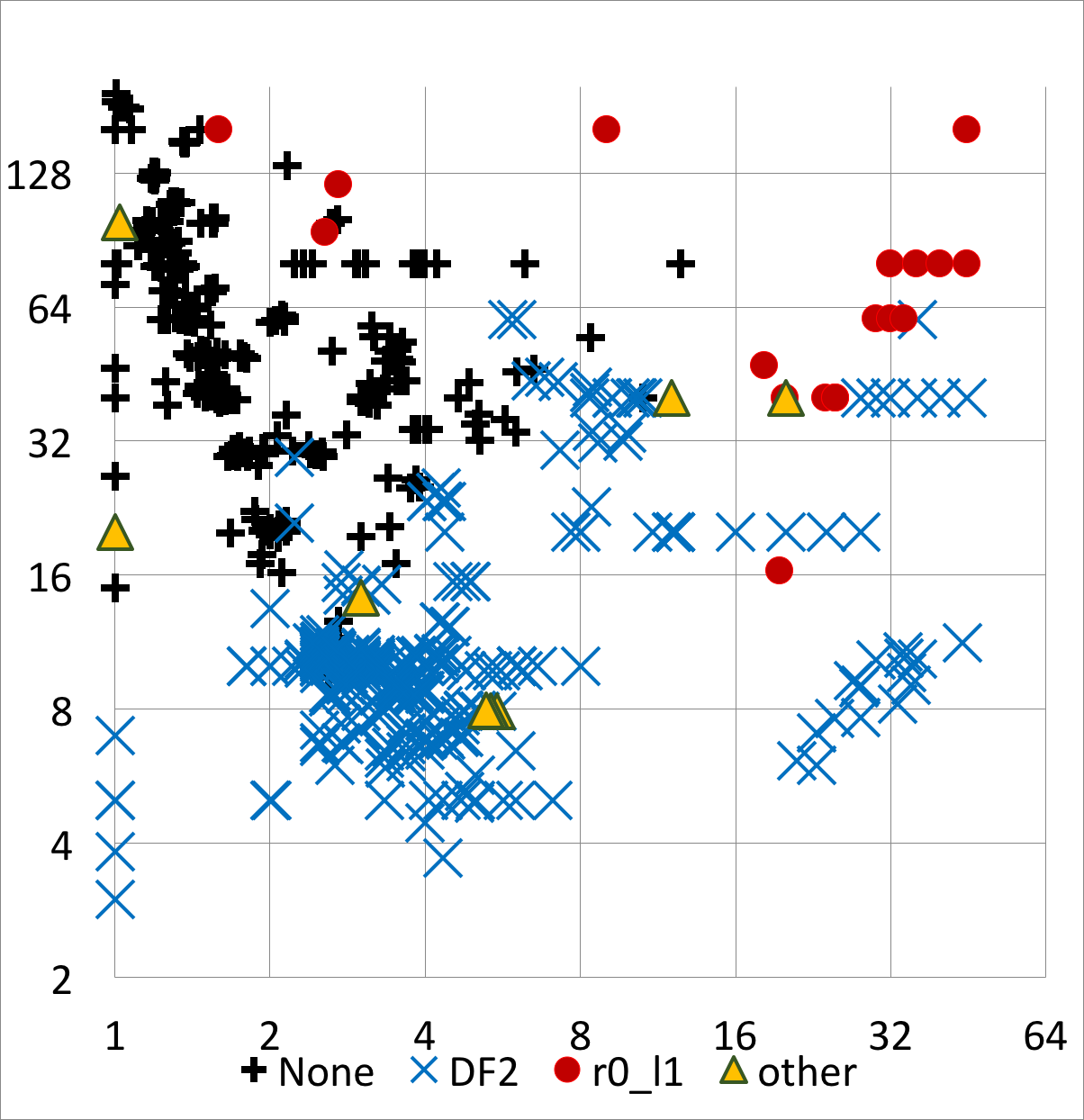
Figure 2: Where None, DF2, and r0_l1 are competitive.

Table 4: Runtime data for instances on the boundaries of our hypotheses.

Instance	spread	nad	None	DF2	r0_l1	r2_l4	min	CPLEX	competitive configs
shown as None in chart but Hypothesis LABEL:hyp:none_dft says DF2 competitive
cl_200_010_080_4	4.9	43.3	2.32	1.41	1.53	5.86	1.21	45.44	None, DF2, r0_l1
blg-200_040_01_05d060	4.6	40	7.74	4.89	6.48	19.44	4.66	238.31	None, DF2, r0_l1
shown as DF2 in chart but Hypothesis 2 says dominance competitive
blg-200_040_16_05d140	28	40	99.28	0.42	0.51	0.89	0.37	1.00	DF2, r0_l1
blg-250_050_16_05d150	30	40	816.18	0.51	0.39	0.85	0.39	2.48	DF2, r0_l1
blg-200_040_16_05d160	32	40	244.71	1.62	1.57	3.92	1.57	3.29	DF2, r0_l1
blg-200_040_16_05d180	36	40	607.35	1.89	1.46	3.34	1.13	4.60	DF2, r0_l1
blg-250_050_16_05d200	40	40	t/o	3.41	3.42	5.83	3.41	15.02	DF2, r0_l1, r2_l4
blg-250_050_16_05d225	45	40	t/o	7.09	7.71	10.52	6.21	17.41	DF2, r0_l1, r2_l4
blg-200_020_16_05d080	16	20	225.73	0.53	0.66	1.59	0.53	1.07	DF2, r0_l1
blg-200_020_16_05d100	20	20	780.26	1.66	1.8	5.95	1.66	3.74	DF2, r0_l1
blg-200_020_16_05d120	24	20	t/o	5.32	5.05	11.01	4.32	11.86	DF2, r0_l1
blg-200_020_16_05d140	28	20	t/o	7.27	8.52	14.80	6.45	12.93	DF2, r0_l1

Fig. 2 shows competitive configs for all 626 goldilocks instances in our general corpus. Each data point shows the first config in the list None, DF2, r0_l1 that is competitive with respect to those in the first two categories of Table 3. This may not be the only competitive one nor the one with minimum runtime. With very few exceptions, all three hypotheses hold. In fact, Table 4 shows that, in the few cases where instances in the chart do not quite meet the numerical thresholds, both of the relevant configs are competitive. There are 12 instances that completely fail to validate the three hypotheses. We address these in detail in Appendix E.

The companion (to Fig. 2) tables in Appendix F show that, not only are the relevant configs competitive, but their runtimes are often close to minimum. In situations where None is competitive (as shown in the chart), it is often better to add degree-1 and/or fold-2 – these have minimal overhead. Where DF2 is competitive, sometimes fold-2 by itself works as well or better. A perusal of the r2_l4 columns reveals that the r2_l4 config is almost never competitive; the same holds for r3_l4, not shown.

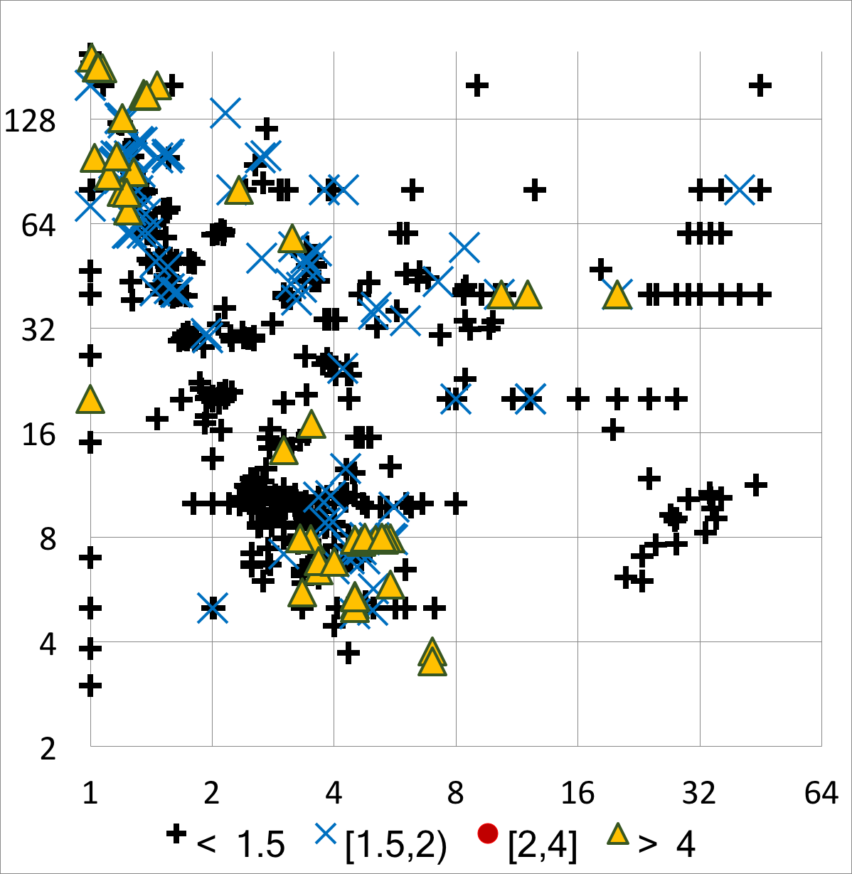
Figure 3: Ratio of r0_l1 runtime to the minimum.

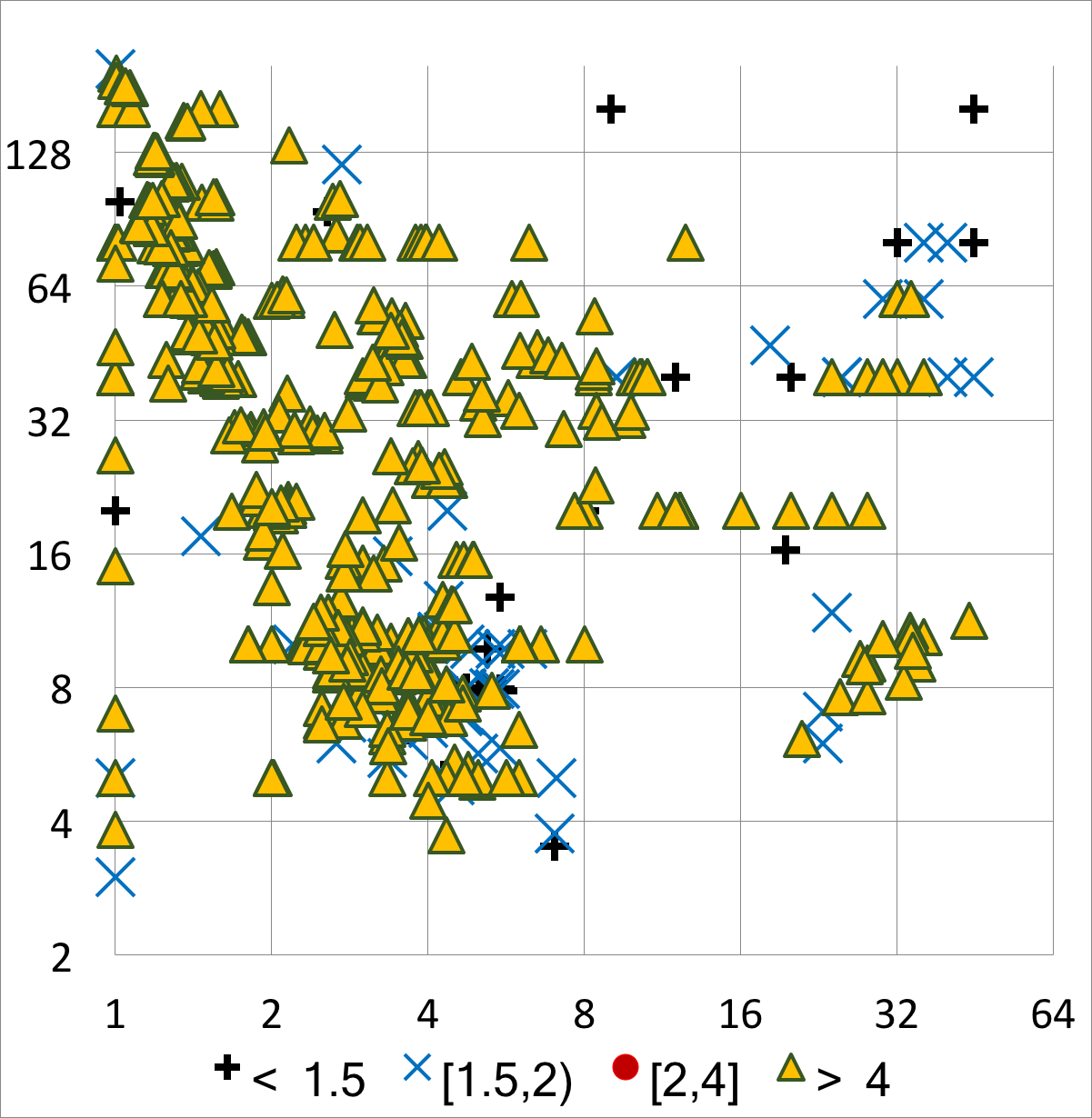
Figure 4: Ratio of r2_l4 runtime to the minimum.

The reader may wonder if the r0_l1 and r2_l4 configs are as good as, or at least competitive, where Hypotheses 1 and 3 apply. Fig. 2 shows that, while r0_l1 is competitive over much of the landscape, there are still many instances where it is not, specifically in regions where None and DF2 are. And lest the reader believe that r2_l4 is competitive in any of the regions specified by the three hypotheses, Fig. 4 shows that r2_l4 is a poor choice for most instances.

5.2 OCT and LP reductions

Table 5: OCT instances where LP reductions are effective.

				runtime				branches
00-Instance	spread	nad	oct %	DF2	r0_l1	r1_l4	CPLEX	DF2	r0_l1	r1_l4	CPLEX
aa41-to-7	24.0	11.8	13.2	t/o	t/o	216.27	4.90	t/o	t/o	365,790	6
aa42-to-7	3.7	6.8	10.8	67.31	89.82	7.19	3.13	496,208	496,173	12,428	26
aa32-to-7	4.7	7.8	18.9	12.48	16.80	6.67	3.38	125,716	125,270	21,628	148
aa29-to-7	4.5	5.4	9.0	51.04	65.76	4.18	2.97	396,403	389,063	5,292	4
aa28-to-7	3.5	7.9	15.9	11.56	14.66	3.99	2.67	103,365	103,199	8,875	50
aa17-to-7	3.7	6.4	14.7	6.97	9.06	3.84	3.59	57,942	57,876	6,606	166
aa24-to-7	5.5	5.9	7.5	30.32	41.20	3.23	2.70	248,317	248,250	4,324	14
aa20-to-7	4.5	5.0	7.8	15.82	18.81	2.71	2.83	132,851	132,628	3,036	29
aa40-to-7	4.4	6.9	15.4	4.45	5.26	2.65	2.15	23,170	23,132	4,161	32
aa19-to-7	4.5	5.1	8.6	6.11	6.49	1.60	2.36	39,821	39,753	2,654	1
aa22-to-7	4.5	5.4	7.8	1.46	1.93	0.41	0.32	5,880	5,874	506	1
aa46-to-7	4.5	4.8	8.9	0.81	0.67	0.38	1.93	2,345	2,325	345	1
aa34-to-7	3.3	5.6	9.3	0.75	0.90	0.32	0.86	3,355	3,334	385	1
aa33-to-7	7.0	3.8	1.5	0.17	0.20	0.05	0.06	344	344	30	1
j20-to-7	7.0	3.5	0.0	0.13	0.17	0.01	0.02	199	199	1	1

Instances are sorted by decreasing r1_l4 runtime.

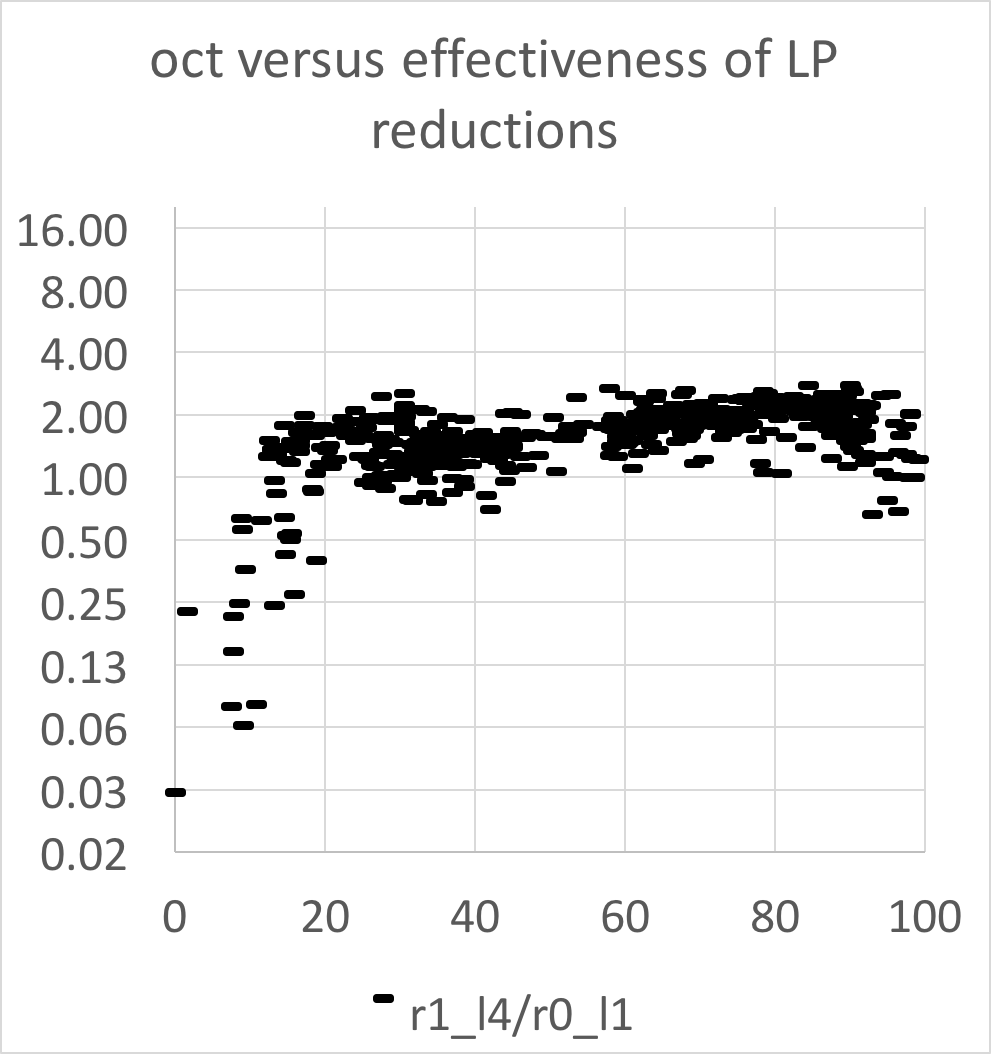
The x-axis is a good oct percentage upper bound; the y-axis represents the ratio between runtime of a config without LP and one with LP added. Up to 20%, adding LP is a good idea. Beyond that, r0_l1 is always within at least a factor of 2.

Figure 5: Effectiveness of LP reductions as a function of estimated oct.

Ho’s thesis [17] proposed another hypothesis.

Hypothesis 4

If (estimated) OCT is small ($<20\%$ of vertices), a config that includes LP, e.g., r1_l4, is competitive.

Since computing OCT directly is an NP-hard problem, we rely on estimates provided by heuristics from [15]. Table 5 shows data for instances in our goldilocks corpus that do not necessarily fit the first three hypotheses, but for which LP reductions lead to significantly lower runtimes. CPLEX is competitive with B&R in all but two instances (instance names in bold); there it spends extra time solving the instance algebraically at the root and its overall runtime is not significant. In one instance, CPLEX is far superior (runtime in bold italic). In all cases, CPLEX does significantly less branching, but more algebraic processing and more cuts. Also, LP by itself with only an LP lower bound is as good as the r1_l4 config for the instances in the table.

The ratio between runtimes for r0_l1 and r1_l4 generally decreases with increasing OCT percentage – estimated OCT as a percentage of vertices; the influence of adding LP reductions and corresponding lower bounds becomes less pronounced as OCT increases. Fig. 5 shows this relationship for the whole corpus.

Interestingly, all of the instances in Table 5 are tunable OCT instances (see Section 4), i.e., randomly generated to mimic instances from the OCT corpus. Except for aa41, the originals were all too easy to be goldilocks.

5.3 Degree of difficulty

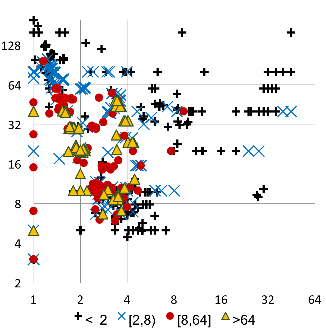
Figure 6: Minimum runtimes (sec) for instances with less than 300 vertices.

It is also important to identify instances where B&R is likely to encounter difficulty. Fig. 6 gives some guidance that, while only small instances are shown, turns out to scale to much larger ones. The main message is that the hardest instances tend to have low to medium average degree and small spread. Conversely, instances with high average degree and/or large spread are easy. None of the instances we report have average degree $<3$; such instances, when small, turn out to be trivial – we address large sparse instances in Section 6.1. This leads to another hypothesis, harder to quantify than the others.

Hypothesis 5

Sparse instances, those with average degree ranging from 5 to 20 (roughly) and small spread, are significantly harder to solve than others.

5.4 Evaluating Hypotheses on PACE Data

Figure 7: Runtime landscape for selected 2019 PACE challenge instances.

Recently we tested our hypotheses on all 200 public instances from the PACE-2019 vertex cover challenge. We used a more powerful server and set a four-hour timeout. For the sake of thoroughness we chose configs None, DF2, r0_l1, Cheap, Cheap+U, Cheap+LP, Cheap+LPU, r0_l1+U, r2_l4, r3_l4, and All.

The instances that VCSolver was able to solve confirmed Hypothesis 3. All were in the region where DF2 should be competitive and all but a few had competitive runtimes for DF2, usually minimum ones. The exceptions are large and, where they are sparse with low spread, required unconfined reductions to reduce them effectively. Table LABEL:tab:pace_table in Appendix F gives results for instances with minimum runtime $>5$ seconds. The instances where DF2 was not competitive are in bold. Table 24 gives degree statistics for the same instances. Here, the instances where r3_l4 has minimum or within 1.5 of minimum runtime are highlighted in bold-italic or bold, respectively.

CPLEX has minimum runtimes on almost all instances where the best runtime for the configs under consideration was more than a second. On the instances with small runtimes, CPLEX preprocessing time dominated the actual branching – they were solved at the root. No config of VCSolver solved any instances beyond vc-exact_100 within our time limit, and only 78 of the first 100 were solved. In contrast, CPLEX was able to solve 142 out of the 200 total instances and 72 of the 100 contest instances.

6 Special Cases

We turn now to instances where our hypotheses do not apply, analyzing these in detail. The main takeaways are (i) large, sparse graphs, if amenable to branch and reduce at all, require a broader suite of reductions – but these are still somewhat predictable; and (ii) graphs with special structure, e.g., geometric and planar graphs, benefit from customized configs.

6.1 Large sparse networks

Table 6: Large sparse real-world instances in the goldilocks zone.

(a) Runtimes for a selection of competitive configurations.

Instance	Cheap+U	Cheap+LP	Cheap+LPU	r2_l4	min	CPLEX
as-skitter	7019.8	17,245.3	8595.3	7922.7	5548.5	6968.1
web-NotreDame	33.4	t/o	31.6	33.2	31.6	num
baidu-relatedpages	2.9	t/o	2.7	2.9	2.7	856.3
libimseti	t/o	468.9	668.1	1651.7	468.9	mem
petster-friendships-dog	t/o	50.3	66.3	59.1	39.1	1487.3
web-Stanford	t/o	t/o	t/o	t/o	38,960.0	num

(b) Degree statistics for the instances.

Instance	n	m	min	b	med	t	max	nad	spread
as-skitter	1,696,415	11,095,298	1	1	5	37	35,455	13.08	37
web-NotreDame	325,729	1,103,836	1	1	2	24	10,721	6.78	24
baidu-relatedpages	415,641	2,374,053	1	1	8	23	127,066	11.42	23
libimseti	220,970	17,233,144	1	1	57	542	33,389	0.14	542
petster-friendships-dog	426,820	8,545,065	1	1	12	105	46,504	0.02	105
web-Stanford	281,903	1,992,636	1	2	6	38	38,625	14.14	19

Time limit was 24 hours or 86,400 seconds. Runtimes are in italics if competitive, bold if within 1.1 of minimum and bold-italic if minimum (usually by a large margin). The libimsetti instance stands out: Cheap+LP outperforms r3_l4 by a factor of more than five. In two of the instances, as-skitter and petster-friendships-dog, a DF2+$x$ config significantly outperformed the corresponding Cheap+$x$ config. These minima are highlighted in the min column of the table. In all but one other case, the difference was slight. However,in the case of libimsetti, the DF2+$x$ configs took almost twice as long as the corresponding Cheap+$x$ configs.

Akiba and Iwata [2] report results for a corpus of sparse real-world networks (Table 1 in their paper). Most of these are either trivial (the instance is reduced at the root with runtimes less than two seconds) or unsuitable for a B&R implementation. In the latter category are the road networks and meshes motivated by graphics, which have average degree between 3 and 6 and spread $<2$, i.e., they confirm Hypothesis 5. Table 6 shows runtime results and degree statistics for five moderately difficult instances and one that is out of reach for all but the full blown r3_l4 config. To accommodate instances of this size we used the more powerful server and a 24-hour timeout.

Large instances make it extremely important to reduce as many vertices as possible at the root, thus decreasing the number of branches (exponential in the number of undecided vertices). Two reductions that are particularly good at this are (i) unconfined, as observed both experimentally – Table 2(a), and theoretically – see Xiao and Nagamochi [28, 29]; and (ii) LP– these are linear time after the $O(m\sqrt{n})$ preprocessing and are unique in their ability to reduce a large number of vertices at once.

It also appears that instances with moderate density and degree spread (web-NotreDame and baidu-relatedpages) favor unconfined reductions, while those that are very sparse with large degree spread (libimseti and petster-friendships-dog) favor LP reductions. The reason for this is unclear. In any case the favored reductions lead to only a small amount of branching. If both unconfined and LP reductions are added to Cheap, we get competitive runtimes for all but the web-Stanford instance.

OCT percentages, below 20% for all of these instances, are misleading – what matters is the OCT value after low degree vertices have been removed by degree-1 and fold-2 reductions. We have not performed this measurement, but the low density and large spread of the two instances that favor LP reductions (libimseti and petster-friendships-dog) suggest that the simple reductions prune a large percentage of vertices.

The first instance, as-skitter (a social network) is hard primarily because of its size – runtimes are in the same two-hour ballpark for all but one config, and for CPLEX. The last instance, web-Stanford, has the nad and spread similar to those of web-NotreDame and baidu-relatedpages, but a more detailed look at its profile in relation to the others reveals some important characteristics: (i) less than 5% of the vertices are degree-1; and (ii) its maximum degree is considerably less, proportionally, than that of baidu-relatedpages (so clique lower bounds are less likely).

The Cheap+LPU, r2_l4, and r3_l4 configs solve petster-friendships-dog without branching and baidu-relatedpages with less than ten branches. Runtimes for all three of these configs are roughly the same on these two instances. This supports our conjecture that eliminating many vertices early is important.

Of special note is the libimseti instance (another social network). It has by far the largest spread and it appears that the presence of many vertices of moderately large degree causes reductions such as dominance and unconfined to be inefficient. The most time consuming reductions for r2_l4 and r3_l4 on this instance are funnel reductions. These are the likely reasons for Cheap+LP to be more than a factor of five faster than r3_l4.

Table 7: Efficiency and effectiveness of reductions on large sparse real-world instances.

(a) Efficiency – microseconds per vertex reduced. The gold column gives the geometric mean for the goldilocks instances in the general corpus. Reductions are sorted by increasing efficiency of the goldilocks instances.

reduction	gold.	as-k	web-N	baidu	libim	pets	web-S
fold2	1.3	1.1	2.4	5.1	161.6	152.0	1.2
deg1	8.1	7.3	2.3	0.8	5.8	1.4	7.3
unconf.	21.6	39.2	52.7	10.9	45,880.2	71.4	24.9
lp	70.0	1,124.8	19.9	5.7	182.2	6.4	112.7
pack.	69.4	13.2	9.2	136,113.0	25,462.9	663,132.0	36.5
fun.	136.3	32.5	647.3	179,117.0	95,881.2	24.7	32.1
twin	117.2	237.6	3.7	52.5	5,135.2	184.1	67.6
desk	129.7	355.4	3.0	301.1	701,832.4	397.6	71.1
dom.	331.7	54.7	37.7	37.2	0.0	37.7	69.2

(b) Effectiveness, the percent of vertices reduced by each reduction. Reductions are sorted by decreasing effectiveness on the goldilocks instances.

reduction	gold.	as-k	web-N	baidu	libim	pets	web-S
fold2	62.4	74.5	26.9	21.9	21.7	46.1	75.9
unconf.	9.9	6.2	2.2	7.0	0.3	3.4	7.1
lp	3.5	0.1	3.1	5.3	74.4	20.4	1.2
pack.	2.4	5.9	1.4	0.0	0.1	0.0	0.4
deg1	1.9	7.5	20.9	64.7	2.6	19.2	6.8
fun.	1.2	3.3	0.1	0.0	0.2	0.0	2.2
desk	0.8	0.3	25.0	0.1	0.0	0.5	3.6
twin	0.5	0.2	18.0	0.5	0.7	10.4	1.6
dom.	0.3	2.0	2.3	0.7	0.0	0.0	1.4

With the exception of the as-skitter and web-Stanford instances, the reduction effeciency/effectiveness profiles of these large sparse instances differs radically from those of the general population. There are more degree-1 reductions – not surprising, but there are significantly fewer fold-2 reductions. The tables clearly point out why Cheap+LP is so effective for libimsetti. LP reductions do most of the work when using the r3_l4 config, on which the data are based, but a lot of time is wasted on unsuccessful packing, unconfined, funnel, and desk reductions.

Finally, note that the config that includes everything except dominance (and packing) is competitive in all but the web-Stanford instance. Table 7 has more detailed information about relative efficiency and effectiveness of reductions on these instances.

6.2 Geometric and Planar Graphs

Two other graph categories that are not amenable to simple configs such as DF2, r0_l1, or Cheap are the geometric and planar graphs we generated.

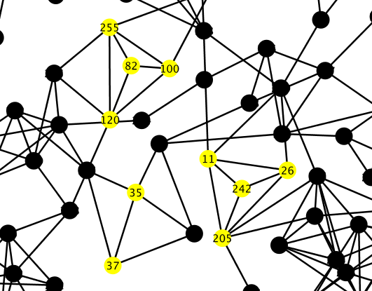
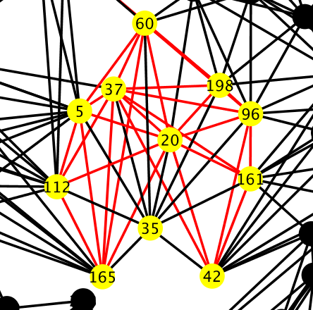
(a) 256 vertices, 512 edges	(b) 256 vertices, 2048 edges

(a) In the sparser geometric graphs there are many $K_{4}$’s with a middle vertex not connected to the rest of the graph or vertices at the junction of two triangles, such as vertex 37. (b) The highlighted vertices and red edges form (at least) three overlapping $K_{5}$’s: vertex sets $\{5,20,37,112,165\}$, $\{20,37,60,96,198\}$ (the edge between 60 and 96 is obscured), and $\{20,37,42,96,161\}$.

Figure 8: Closeup view of two geometric graphs.

Table 8: Runtime and branching data for harder 512-vertex geometric instances.

Instance	edges	spread	runtime				branches
			DD	r0_l1+U	r3_l4	CPLEX	DD	r0_l1+U	r3_l4	CPLEX
W-16384-0	15,968	1.4	900.0	900.0	707.3	4.5	2,723,618	927,514	280,594	80
W-16384-1	15,868	1.4	900.0	900	567.8	3.4	2,790,936	950,663	237,319	27
W-16384-4	15,920	1.4	900.0	900	485.2	3.0	3,064,004	1,040,497	198,080	51
W-16384-3	16,118	1.6	900.0	900.0	420.8	4.0	3,125,229	1,028,770	176,676	85
W-16384-2	16,020	1.7	900	900	372.7	4.8	3,396,657	1,042,980	161,528	185
W-08192-0	7,026	2.5	22.0	1.2	1.3	0.5	272,410	868	328	7
G-08192-0	7,026	2.5	22.4	1.1	1.2	0.5	272,410	868	328	7
W-04096-2	3,954	2.6	225.7	1.3	1.1	0.4	2,497,458	1,234	400	0
G-08192-1	7,046	2.2	22.2	1.1	1.0	0.5	279,029	1,088	290	5
W-08192-1	7,046	2.2	21.9	1.1	1.0	0.5	279,029	1,088	290	5
W-04096-3	3,933	2.6	900	1.9	0.9	0.0	11,460,458	1,262	228	417
W-08192-3	7,188	2.6	10.8	0.7	0.8	0.4	94,997	378	134	0
G-16384-4	13,623	2.2	2.1	0.8	0.8	0.3	11,661	440	136	0
G-08192-3	7,188	2.6	10.7	1.7	0.7	0.4	94,997	378	134	0
G-08192-2	7,161	2.7	13.0	0.6	0.7	0.6	179,228	430	150	9
W-08192-2	7,161	2.7	12.9	0.5	0.6	0.6	179,228	430	150	9
G-16384-3	13,547	2.7	0.7	0.4	0.6	0.5	2,806	80	72	0
W-04096-4	3,944	2.6	209.0	0.6	0.5	0.2	1,686,029	274	60	0
G-16384-2	13,528	2.6	0.7	0.4	0.4	0.6	4,791	62	60	0
G-16384-0	13,346	2.3	1.1	0.2	0.5	0.3	4,266	62	54	0
W-04096-0	3,771	2.2	24.8	0.1	0.2	0.2	267,644	84	42	0
G-08192-4	7,205	2.6	15.2	0.1	0.1	0.9	145,475	50	30	158
W-08192-4	7,205	2.6	15.4	0.1	0.1	0.9	145,475	50	30	158
G-04096-0	3,611	2.8	1.0	0.1	0.1	0.3	12,868	26	23	0
G-04096-3	3,747	3.1	7.8	0.1	0.1	0.1	129,550	28	20	0
W-04096-1	3,922	2.4	124.1	0.1	0.1	0.4	1,752,487	32	14	3
G-16384-1	13,291	2.2	0.4	0.1	0.1	0.2	1,576	10	10	0

The ’W’ instances are geometric graphs with wraparound, e.g., points at distance $d$ from the left edge of the unit square are treated as if they were distance $d$ to the right of the right edge. The ’G’ instances have no wraparound. Instance numbers reflect the desired number of edges – actual number of edges differ from these. The configs that do not include dominance timed out on these instances and r3_l4 always performed at least as well as r2_l4. Except for the easier instances, CPLEX has the best runtimes, but we indicate the best runtimes among the VCSolver configs in bold italics nonetheless.

Geometric graphs. Table 8 shows data for the harder 512-vertex geometric graphs. Any config that did not include dominance reductions timed out on all instances and the full suite provided by r3_l4 gave the best runtimes.

For the sparsest geometric graphs, not shown in the table (runtimes for competitive configs were less than $1/100$ second), dominance is effective on its own because there are many dominated degree-3 vertices – see Fig. 8(a). In the mid-range, Fig. 8(b), CPLEX is the better choice; the neighborhood of most vertices does not yield opportunities for dominance or even unconfined reductions; and the induced cliques overlap. At the highest densities, also not shown, there are enough large cliques so that dominance can reduce the graph at the root.

All of these instances are easy for CPLEX – the only reason it does not always have the best runtimes is because of preprocessing at the root.

Table 10 shows that the profile of reduction effectiveness is radically different for geometric graphs than for the general population. The dominance and unconfined reductions play a much more pronounced role. Profiles of easier geometric instances are also shown – there, degree-1, dominance, and fold-2 reductions, the ones composing r0_l1, do almost all the work.

Table 9: Runtime and branching data for planar and 3-regular graphs.

	runtime				branches
Instance	r0_l1+FU	r2_l4	r3_l4	CPLEX	r0_l1+FU	r2_l4	r3_l4	CPLEX
tri_inf-1000_9	169.3	207.8	24.4	5.9	100,179	200,689	16,353	383
tri_inf-1000_4	6.2	11.0	4.7	2.2	3,757	7,500	2,137	0
tri_inf-1000_2	0.4	0.6	0.5	3.9	107	211	151	170
tri_inf-1000_6	0.6	1.0	0.4	3.3	122	245	73	3
tri_inf-1000_3	1.0	1.4	0.7	9.2	172	345	117	1,712
tri_inf-1000_0	0.4	0.5	0.4	2.9	68	137	63	0
tri_inf-1000_8	0.3	0.5	0.5	2.6	48	97	83	0
tri_inf-1000_1	0.1	0.2	0.2	1.9	22	45	43	0
tri_inf-1000_5	0.2	0.3	0.4	3.4	42	85	75	158
tri_inf-1000_7	0.1	0.2	0.1	29.9	25	51	35	4,261

(a) Full triangulations, including infinite face.

	runtime				branches
Instance	Cheap+FU	r2_l4	r3_l4	CPLEX	Cheap+FU	r2_l4	r3_l4	CPLEX
dual_1024-4	15.0	17.7	9.8	1.8	19,951	8,565	4,205	6
dual_1024-6	13.3	15.4	9.2	2.5	16,107	7,113	3,695	0
dual_1024-1	14.5	14.3	8.2	2.7	16,076	6,891	3,665	139
dual_1024-9	13.9	17.0	6.8	2.0	15,119	6,761	2,667	50
dual_1024-5	8.0	9.8	4.0	2.4	8,559	3,559	1,333	0
dual_1024-2	9.2	10.1	3.3	2.5	10,169	4,378	1,227	29
dual_1024-8	5.6	6.1	4.9	3.0	6,227	2,071	1,128	331
dual_1024-3	10.5	11.7	3.4	1.5	12,665	5,272	1,077	0
dual_1024-7	3.8	3.8	1.7	3.1	2,036	838	285	77
dual_1024-0	1.6	2.5	1.4	2.1	921	407	192	21

(b) Duals of full triangulations.

	runtime				branches
00-Instance	DF2	r2_l4	r3_l4	CPLEX	DF2	r2_l4	r3_l4	CPLEX
reg3-300_4	6.8	12.2	12.2	4.2	112,353	32,701	24,548	3,446
reg3-300_2	6.7	10.0	10.1	7.3	103,040	24,301	19,696	7,542
reg3-300_9	6.6	9.8	10.4	11.3	84,795	22,361	17,263	10,516
reg3-300_7	6.3	10.0	10.0	13.0	101,756	24,074	19,184	11,697
reg3-300_5	6.0	10.8	10.0	20.1	86,157	24,505	18,507	22,569
reg3-300_3	5.6	5.7	7.1	5.9	67,051	12,998	10,831	5,678
reg3-300_8	5.3	8.2	7.1	8.6	71,221	19,058	14,043	7,127
reg3-300_0	5.2	6.8	6.3	15.0	74,005	13,164	9,999	10,739
reg3-300_1	5.0	7.8	8.0	9.0	72,186	18,631	15,087	5,569
reg3-300_6	4.4	6.5	6.8	9.2	55,902	12,234	9,455	8,417

(c) 3-regular graphs with 300 vertices.

For the two types of planar instances unconfined reductions play a key role; performance is even better when funnel reductions are included. For the harder instances, packing appears to be a major factor. The desk reduction plays an important role in the duals – any degree-4 vertex in the original graph leads to a chordless 4-cycle in the dual. CPLEX also does well on these instances.

Planar graphs. While complete Delaunay triangulations are not necessarily representative of maximal planar graphs, nor are their duals representative of 3-regular planar graphs, these two classes do illustrate another situation necessitating more complex configs.

The full triangulations – Table 9(a), are remarkable in their wide range of difficulty. All have the same number of edges, 2994, and almost exactly the same degree spread, 2. We ran r3_l4 on 30 different permutations (vertices renumbered, edges reordered) of the most difficult instance, tri_inf-1000_9, and found (only) a factor of two difference between minimum and maximum runtime with a small standard deviation (roughly 3). There was even less variance for the easiest instance, tri_inf-1000_7. So the difference must lie in subtle structural properties, such as higher degree vertices with degree-3 neighbors, leading to degree-2 reductions (fold-2 or dominance on degree-2 vertices).

The duals – Table 9(b), are less prone to varying runtimes, but still more so than can be accounted for by input permutation. Statistics for permuted runs are almost identical to those of the full triangulations. And nothing stands out when looking at differences in efficiency and effectiveness of reductions. Table 9(c) shows runtimes for 300-vertex 3-regular graphs, which have comparable runtimes but are much smaller. Simple reductions suffice here and runtimes vary much less.

Table 10: The median effectiveness and efficiency of various reductions on geometric and planar graphs versus comparable other graphs.

reduction $\mu$sec/vertex % reduced med geo med geo fold2 5.0 4.6 49.9 45.9 dom. 36.0 36.4 19.2 21.2 unconf. 105.9 107.5 20.9 19.9 deg1 16.6 16.0 6.1 6.0 pack. 260.6 265.2 1.1 1.0 fun. 382.3 463.7 0.8 0.6 desk 448.5 395.7 0.7 0.8 twin 423.3 419.5 0.3 0.2 lp 1,234.5 1,379.4 0.3 0.3	reduction $\mu$sec/vertex % reduced med geo med geo dom. 7.4 11.6 42.2 47.5 fold2 6.3 11.7 39.5 18.7 deg1 19.3 22.8 14.5 9.8 fun. 3.0 3.8 $<0.1$ $<0.1$ unconf. 3.0 5.4 $<0.1$ $<0.1$ pack. 11.0 18.4 $<0.1$ $<0.1$ lp 36.0 43.1 $<0.1$ $<0.1$ twin 249.0 352.6 $<0.1$ $<0.1$ desk 412.0 385.3 $<0.1$ $<0.1$
(a) Harder geometric instances. 512 vertices, average degree 16 and 32.	(b) Easier geometric instances. 512 vertices, average degree 4, 8 and 64.
reduction $\mu$sec/vertex % reduced med geo med geo fold2 2.5 2.3 69.4 69.1 unconf. 84.0 80.8 13.5 13.7 dom. 47.3 37.5 7.7 8.0 deg1 18.1 15.1 6.2 6.1 fun. 138.3 117.6 1.7 1.6 desk 357.2 599.2 0.3 0.3 pack. 209.7 240.4 0.3 0.2 twin 540.8 975.7 0.2 0.1 lp 1,746.5 2,431.3 0.1 0.1	reduction $\mu$sec/vertex % reduced med geo med geo fold2 0.7 0.9 75.1 75.2 desk 29.7 33.1 7.9 8.2 unconf. 25.3 28.2 7.0 6.9 deg1 4.2 4.7 6.0 6.0 fun. 27.5 26.3 2.4 2.3 dom. 61.4 72.8 1.0 1.0 lp 2,479.7 2,484.2 0.1 0.1 twin 756.0 698.6 0.1 0.1 pack. 148.6 213.5 0.1 0.1
(c) Planar: Full triangulations. 1000 vertices, 2994 edges.	(d) Duals of full triangulations. 1024 vertices, 1536 edges, 3-regular.
reduction $\mu$sec/vertex % reduced med geo med geo fold2 1.2 1.3 71.2 62.4 unconf. 24.6 21.6 9.1 9.9 lp 51.5 70.0 4.5 3.5 pack. 59.4 69.4 3.5 2.4 deg1 6.1 8.1 2.8 1.9 fun. 81.8 136.3 2.0 1.2 desk 108.5 129.7 0.8 0.8 twin 96.3 117.2 0.5 0.5 dom. 236.8 331.7 0.3 0.3	reduction $\mu$sec/vertex % reduced med geo med geo fold2 0.3 0.3 89.7 89.6 deg1 3.6 3.7 3.0 3.0 fun. 16.0 16.3 2.6 2.6 unconf. 23.3 23.3 2.0 2.0 desk 73.8 72.8 1.0 1.0 pack. 11.2 11.8 0.9 0.9 lp 347.5 292.2 0.4 0.4 dom. 107.4 125.8 0.2 0.2 twin 167.5 207.9 0.2 0.2
(e) General corpus – see Table 2: 626 goldilocks instances.	(f) 3-regular graphs: 300 vertices, 450 edges.

In all tables, reductions are sorted by decreasing frequency (geometric means).

Table 10 shows relative efficiency and effectiveness of reductions for geometric, planar, and 3-regular graphs in comparison with the main goldilocks corpus. We have already discussed geometric graphs. Duals of triangulations have profiles very similar to 3-regular graphs, except for the importance of desk reductions in the former: a vertex of degree four in the original triangulation leads to a chordless 4-cycle in the dual. And 3-regular graphs differ from the general population in that LP reductions are neither efficient nor effective in the former. Nor are they efficient/effective in any of the geometric or planar classes. Finally, the full triangulations differ mostly from the 3-regular ones in the prominence of dominance reductions. The triangulations, like the sparse geometric graphs, are likely to have $K_{4}$’s with an ’unconnected’ middle vertex – see Fig. 8(a).

7 Conclusions and Future Work

Using a large corpus of problem instances from multiple sources we have validated hypotheses that allow a B&R solver (automated or with human guidance) to conclude when to (i) use no reductions at all; (ii) use the simplest reductions (degree-1, fold-2) only; and (iii) use more sophisticated reductions such as dominance, unconfined, and LP. We have formulated five hypotheses and tested them on our randomly generated instances, several benchmark collections, and instances from the recent PACE challenge.

Our study raises many questions and offers opportunity for new avenues of investigation. A C++ solver based on VCS+ was used in our early experiments – we are now poised to add sophistication to it. Here are some ideas for future work.

• Solutions produced early by VCSolver are usually close to optimal; future experiments can address how it fares as an ’anytime algorithm’ (use the best solution produced within a given time limit), compared with metaheuristics (see, e.g., Andrade et al. [3]), particularly on large instances where optima are not known.

• VCS+ does not currently provide a mechanism for changing the order of the reductions; our experiments suggest that, for most instances, fold-2 should be early in the sequence and dominance later (see Algorithm 3 in Appendix A for the VCSolver sequence).

• Automation appears to be a promising prospect; given what we know about both the larger and the small/medium instances, it makes sense to apply the Cheap+LPU config at the root and then measure the instance (or instances if there are multiple components) to determine how to proceed.

• Runtime for dominance depends on the degrees of the vertices under consideration. It may make sense, for some graphs (characteristics need to be determined experimentally), to set a threshold for the degree of vertices considered as dominated. In other words, restrict the search to vertices $v$ of degree $\leq d$ and, for each such $v$, check whether it is dominated by any of its neighbors.

Acknowledgement. The authors thank Yoichi Iwata for his help navigating some of the details of VCSolver, and for providing insights about the LP reduction that allowed us to create a stand-alone implementation.

A Branch and reduce algorithm

Here we show the details of VCSolver in three main parts. The first, Algorithm 1 is the basic branching strategy. Variable $I$ represents a (sub)instance and $|I|$ is the number of vertices in $I$. When a branching vertex $v$ is chosen, one subinstance includes $v$ in the cover and the other omits $v$, but includes all its neighbors. We use max-degree branching – always choose a vertex of maximum degree. VCSolver does not create new instances: only one copy of the graph is maintained and vertices are marked in a status vector as in, out, or undecided depending on whether, based on decisions leading to the current branch, they are known to be in the cover, not in the cover or still part of the current instance. When branching creates smaller instances, a stack keeps track of only the vertices whose status has changed. Thus there is also only one copy of the status vector. Small additional status vectors keep track of vertices introduced during folding.

Algorithm 2 is responsible for applying reductions (using Algorithm 3) and deciding what to do with the current node, which is either the root (original instance) or a branch. Both of these functions have an option for brute force solution when the instance is sufficiently small. ProcessNode is also alerted when the graph becomes disconnected. The procedure ComponentSolve hides these details.

Reduce applies reductions in a fixed order (our VCS+ does not change this) and, if any reduction reduces at least one vertex, the sequence starts at the beginning. For example, if degree-One, dominance, and unconfined fail, and lp succeeds, then degree-1 reductions are applied again, etc. A reduction is applied only if selected by its runtime option.

Algorithm 1 A branching algorithm for minVC.

function Solve($I,C$)

     $\textsl{status}\leftarrow\textsc{ProcessNode}(I)$

     if status = solved then

         $C\leftarrow\min(|I|,C)$

     end if

     if status = alive then

         save vertex status vector on stack

         $x\leftarrow\textsc{Select-Branching-Candidate}(I)$

         $C_{l}\leftarrow\textsc{Solve}(I\setminus\{x\},C-1)$

         restore status vector and save it again

         $C_{r}\leftarrow\textsc{Solve}(I\setminus N[x],C)$

         restore status vector

         $C\leftarrow\min\{C,C_{l}+1,C_{r}\}$

     else if status = solved then

         $C\leftarrow\min(|I|,C)$

     end if

     return $C$

end function

Algorithm 2 Processing the root/branch.

function ProcessNode($I$)

     $\textsl{n}\leftarrow\text{\# of vertices in the graph}$

     $\textsl{undecided}\leftarrow\text{\# of undecided vertices}$

     status $\leftarrow$ Reduce(I)

     if $\textsl{status}=$ reduction_cut then return solved

     if $\textsl{undecided}=0$ then

         return solved

     end if

     if I not connected then

         solve components separately

         return solved

     else if undecided is small then

         solve by brute force

         return solved

     end if

     return alive

end function

Algorithm 3 Applying reductions.

function Reduce($I$)

     $\rhd$ Each reduction function returns

     $\rhd$ true if at least one vertex is reduced,

     $\rhd$ false otherwise

     $\textsl{n}\leftarrow\text{\# of vertices in the graph}$

     $\textsl{undecided}\leftarrow\text{\# of undecided vertices}$

     while $\textsl{undecided}>0$ do

         if degree-one(I) then continue

         $\rhd$ if # undecided vertices below threshold,

         $\rhd$ solve by brute force

         if $\textsl{n}\cdot\textsl{SHRINK}\geq\textsl{undecided}$ then

              $\textsc{Component-Solve}(\textsl{I})$

              return reduction_cut

         end if

         if dominance(I) then continue

         if unconfined(I) then continue

         if lp(I) then continue

         if packing(I) then continue

         if fold2(I) then continue

         if twin(I) then continue

         if funnel(I) then continue

         if desk(I) then continue

         break

     end while

     if $|I|=0$ then return reduction_cut

     return alive

end function

B Options and Statistics Provided by VCS+

Table 11: Options provided by VCS+

  -b, --branching <int>(2)Ψ0: random, 1: mindeg, 2: maxdeg
  -d, --debug <int>(0)Ψ0: no debug output, 1: basic branching and decompose,
                        2: detailed branching and decompose and basic reduction,
                        3: detailed reduction
  -t, --timeout <int>(3600)Ψtimeout in seconds
      --trace <int>(0)Ψ0: no trace, 1: short version without solution vectors,
                        2: full trace with solution vectors
      --quiet <boolean>(false) Don’t print progress messages
      --root <boolean>(false)ΨOnly process root node -- no branching
      --show_solution <boolean>(false)ΨEnable printing of solution vector
      --clique_lb <boolean>(false)ΨEnable clique lower bound
      --lp_lb <boolean>(false)ΨEnable lp lower bound
      --cycle_lb <boolean>(false)ΨEnable cycle lower bound
      --deg1 <boolean>(false)ΨEnable degree1 reduction
      --dom <boolean>(false)ΨEnable dominance reduction
      --fold2 <boolean>(false)ΨEnable fold2 reduction
      --LP <boolean>(false)ΨEnable LP reduction
      --unconfined <boolean>(false)ΨEnable unconfined reduction
      --twin <boolean>(false)ΨEnable twin reduction
      --funnel <boolean>(false)ΨEnable funnel reduction
      --desk <boolean>(false)ΨEnable desk reduction
      --packing <boolean>(false)ΨEnable packing reduction
      --all_red <boolean>(false)ΨEnable all reductions except packing,
                                    equivalent to old ’-r2 -l3’
      --helpΨShow this message
  

Table 12: Statistics printed by VCS+

num_vertices        Ψ             510
num_edges           Ψ            4032
value               Ψ             412
runtime             Ψ     3.595
num_branches        Ψ            5682
Reduction Times (ms):
deg1Time            Ψ    41.760
domTime             Ψ   329.665
fold2Time           Ψ   144.886
lpTime              Ψ   248.026
twinTime            Ψ    80.137
deskTime            Ψ   260.051
unconfinedTime      Ψ  1401.675
funnelTime          Ψ   303.038
packingTime         Ψ     0.000
Vertices Reduced:
deg1Count           Ψ           10956
domCount            Ψ            8321
fold2Count          Ψ          161319
lpCount             Ψ           18254
twinCount           Ψ             843
deskCount           Ψ            2793
unconfinedCount     Ψ           84497
funnelCount         Ψ            7833
packingCount        Ψ               0
Effective Reduction Calls:
deg1Calls           Ψ            3239
domCalls            Ψ            4010
fold2Calls          Ψ           16402
lpCalls             Ψ            3531
twinCalls           Ψ             167
deskCalls           Ψ             287
unconfinedCalls     Ψ           15179
funnelCalls         Ψ            2437
packingCalls        Ψ               0
Total Reduction Calls:
deg1AllCalls        Ψ           30097
domAllCalls         Ψ           19311
fold2AllCalls       Ψ           53388
lpAllCalls          Ψ           17343
twinAllCalls        Ψ           36986
deskAllCalls        Ψ           36819
unconfinedAllCalls  Ψ           32522
funnelAllCalls      Ψ           13812
packingAllCalls     Ψ               0
Effective Lower Bounds:
trivialLBCount      Ψ            4933
cliqueLBCount       Ψ             736
lpLBCount           Ψ              11
cycleLBCount        Ψ               0
Lower Bound Times (ms):
cliqueLBTime        Ψ   220.685
cycleLBTime         Ψ     0.000
num_leftcuts        Ψ               2
root_lb             Ψ             380
  

Table 11 shows the options provided by VCS+. Almost all of these are related to selecting specific reductions and lower bounds. The order of application for the reductions is not affected, i.e., the order of the relevant options on the command line makes no difference.

Table 12 shows the important part of the output of VCS+ (header information giving version, date, input file name, options, etc., is omitted). The most useful data are the runtimes and number of vertices reduced by each reduction. Also provided are runtimes for lower bounds and number of times each lower bound was effective in cutting off a branch and information about how many times the procedure invoking each reduction was called and how many times it succeeded in reducing at least one vertex.

At the end of the output is a string of 0’s and 1’s representing the solution found by VCS+: a 1 in position $i$ if vertex $i$ is included, a 0 if not. Indexing is 0-based (some benchmark instances have vertices numbered 0) and an underscore (_) is used for missing vertices (aside from a missing 0-vertex some benchmarks have non-contiguous numbering). We provide a script for verifying solutions in this format.

C DIMACS challenge instances

In this appendix, we describe the provenance of the DIMACS instances. Although these instances were originally used for the minimum coloring problem, Akiba and Iwata [2] use the complement graphs of these instances in their experiments. To maintain consistency between our results and theirs, we also use the complement graphs. There are three types of DIMACS instances: (i) random graph generators based on the Erdos-Renyi models, (ii) random graph generators that embed a clique, and (iii) graphs taken from applications.

Random. The C and DSJC instances are based on the $G(n,p)$ Erdos-Renyi model – a graph of $n$ vertices where each edge has probability $p$ being added independent from every other edge. The C instances were created by Michael Trick using a graph generator written by Craig Morgenstern. The DSJC instances were used by Johnson et al. [19] in simulated annealing experiments for graph coloring and number partitioning. The naming convention for these two types are C$n.p$ and DSJC$n.p$ where $n$ and $p$ are the parameters of the $G(n,p)$ model.

$X$	$a=$	$b=$	Expected Density
1	0.00	0.50	0.25
2	0.00	1.00	0.50
3	0.50	1.00	0.75

Table 13: Parameter values for p_hat$n$-$x$ instances

The p_hat instances use the p_hat generator introduced by Gendreau et al. [12], using a generalization of the $G(n,p)$ model that accepts three parameters: $n$, the number of vertices; $a$ and $b$ which are both real numbers such that $0\leq a\leq b\leq 1$. Each vertex $x$ is assigned a value $a\leq p[x]\leq b$ – the probability that an edge $uv$ is added is $\frac{1}{2}(p[u]+p[v])$. When $a=b$, the p_hat model is equivalent to the $G(n,p)$ model. The p_hat instances use the following naming convention: p_hat$n$-$x$ where $n$ is the number of vertices, and $x$ denotes a combination of values for $a$ and $b$ (see Table 13 for specific parameter values).

The sanr instances are random graphs that generated using the procedure introduced by Sanchis and Jagota [25].

Embedded clique. The brock instances use the DELTA generator written by Mark Brockington and Joe Culberson. The Brock instances use the following naming convention: brock$n$_$x$ where $n$ is the number of vertices and $x$ is a distinguishing tag.

The san generator, created by Sanchis and Jagota [25], accepts three parameters: $n$, the number of vertices; $m$, the number of edges; and $c$, the size of the embedded clique. The following naming convention is used: san$n$_$d$_$r$ where $n$ is the number of vertices, $d$ is the density, and $r$ is an integer used to distinguish instances with the same number of vertices and edges but different embedded clique sizes.

Other. The c-fat instances are taken from Berman and Pelc’s [5] work on fault diagnosis for multiprocessor systems. For a given parameter $c$, a $c$-fat ring is a graph, $G=(V,E)$, constructed as follows: Let $k=\left\lfloor\frac{|V|}{c\mathrm{log}|V|}\right\rfloor$ and $W_{0},...,W_{k-1}$ be a partition of $V$ such that $c\mathrm{log}|V|\leq|W_{i}|\leq 1+\left\lceil c\mathrm{log}|V|\right\rceil$ for all $i=0,...,k-1$. For each $u\in W_{i}$ and $v\in W_{j}$, add the edge $uv$ if $u\not=v$ and $|i-j|\in\{0,1,k-1\}$. Naming convention is: c-fat$n$-$c$ where $n$ is the number of vertices and $c$ is the construction parameter.

The MANN instances are based on Steiner triples. For a set $S=\{1,\ldots,n\}$, a Steiner triple system of $S$ is a set $F_{S}=\{T_{1},...,T_{m}\}$ where $T_{i}\subset S$ and $|T_{i}|=3$ (we call $T_{i}$ a Steiner triple), such that for every $u,v\in S$, $u$ and $v$ are contained in exactly one $T_{i}$. It is known that a Steiner triple system exists if and only if $n\geq 3$ and $n\equiv 1,3$ (mod 6) [11]. To construct a MANN graph from a Steiner triple system, add a vertex $v_{s}$ for each $s\in S$. Then for each Steiner triple $T=\{i,j,k\}$, add a clique of size 3 and let $t_{i}$, $t_{j}$, $t_{k}$ be the associated vertices. For each $s$, add an edge between $v_{s}$ and $T_{s}$ for all Steiner triples that contain $s$. The resulting graph is a set of triangles connected by high degree ($>3$) vertices. We use MANN_a$n$ to denote a MANN graph constructed from a Steiner triple system of $\{1,\ldots,n\}$.

D OCT instances

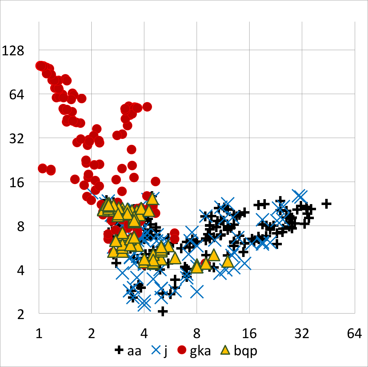
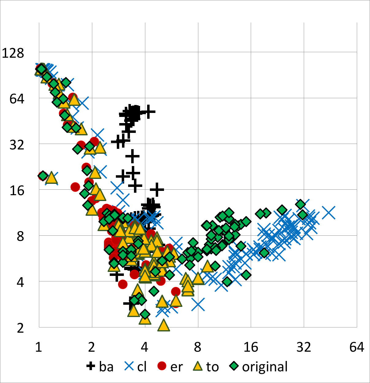
(a) Oct instance categories on our landscape: the aa and j instances come from the genetic database published by Wernicke [27], the gka from the dataset used by Glover et al. [13], and the bqp instances are from from Beasley’s OR library.	(b) Synthetic oct instances on our landscape, generated to have roughly the same size, density, and oct percentages as the originals. The generators used are Barabasi-Albert (ba), Chung-Lu (cl), Erdös-Renyi ((er)), and tunable oct (to). See Goodrich et al. [14].

Figure 9: Oct and synthetic versions on our landscape.

Fig. 9 shows the distribution of the OCT instances and their synthetic derivatives on our landscape. None of these instances have both large degree and wide spread. The synthetic versions, as expected, track the originals pretty well – they are designed to have roughly the same average degree. Barabasi-Albert graphs, while guaranteed to be connected, have less control over degree spread.

E Exceptions to the main hypotheses

Table 14: Exceptions to our hypotheses.

Instance	None	DF2	r0_l1	r0_l1+U	r2_l4	min	cpx	config	br-conf	br-cpx
ba_512_008_3	t/o	0.21	0.16	0.07	0.11	0.07	2.10	r0_l1+U	4	0
ba_512_008_5	t/o	0.19	0.15	0.06	0.10	0.06	0.54	r0_l1+U	4	0
ba_999_008_5	t/o	1.43	1.23	0.47	0.90	0.47	5.97	r0_l1+U	55	0
blg-200_020_16_05d020	9.88	11.23	5.05	2.33	3.42	2.33	0.02	r0_l1+U	1,516	0
blg-200_040_16_05d060	3.56	0.42	0.39	0.05	0.05	0.05	0.05	r0_l1+U	0	0
blg-200_120_20_07d199	2.66	0.93	0.02	0.02	0.03	0.02	0.17	r0_l1	48	78
blg-200_160_01_03d199	1.25	1.06	0.50	0.76	1.50	0.49	10.85	r0_l1	1,441	405
blg-250_050_16_05d100	2.17	0.36	0.17	0.05	0.05	0.05	0.05	r0_l1+U	0	0
blg-250_200_16_05d225	3.01	2.35	0.03	0.03	0.03	0.02	0.11	DD	0	0
DSJR500.1	t/o	t/o	6.38	0.82	0.38	0.38	0.36	r2_l4	125	0
DSJR500.5	1.78	2.03	0.14	0.10	0.13	0.10	0.52	r0_l1+U	0	0
gka_16	2.17	1.04	0.35	0.04	0.05	0.04	0.07	r0_l1+U	0	6

(a) The config column shows the config with the fewest reductions that comes within 1.1 of the minimum. Runtimes for all such configurations are shown in bold italics. Bold runtimes are competitive. The cpx column shows CPLEX runtimes. The br-conf and br-cpx columns show the number of branches for the minimum runtime configuration and CPLEX, respectively.

Instance	n	m	min	bottom	med	mean	top	max	stdev	spread	nad
ba_512_008_3	512	2,032	4	4	5	7.9	22	79	7.7	5.5	7.9
ba_512_008_5	512	2,032	1	4	5	7.9	21	85	8.1	5.4	7.9
ba_999_008_5	999	3,980	1	4	5	8.0	21	125	8.8	5.3	8.0
blg-200_020_16_05d020	200	2,000	10	20	20	20.0	20	25	1.2	1.0	20.0
blg-200_040_16_05d060	200	4,000	5	5	60	40.0	60	60	25.0	12.0	40.0
blg-200_120_20_07d199	200	12,000	71	73	76	120.0	199	199	59.3	2.7	120.0
blg-200_160_01_03d199	200	16,000	121	125	157	160.0	199	199	26.5	1.6	160.0
blg-250_050_16_05d100	250	6,250	5	5	18	50.0	100	100	44.0	20.0	40.0
blg-250_200_16_05d225	250	25,000	5	5	225	200.0	225	225	64.7	45.0	160.0
DSJR500.1	500	3,555	4	7	14	14.2	21	25	4.4	3.0	14.2
DSJR500.5	500	58,862	103	142	231	235.4	363	388	64.7	2.6	94.2
gka_16	180	8,016	87	88	89	89.1	90	90	0.9	1.0	99.0

(b) Degree statistics for the exceptions. The instances where adding dominance is important are in bold. The one where the full suite of reductions appears to be necessary, DSJR500.1, is in italics. The rest rely primarily on unconfined reductions.

In Fig. 2 there are three red dots in the region where None should be competitive and nine scattered instances where the simplest configs are not competitive. Table 14 gives runtime and degree data for all 12 exceptions.

The first three ba instances are easy for all configs except None, and DF2 is competitive when measured against r2_l4. The last blg instances, where dominance is a major factor (bold), are unusual in that at least 5% of vertices also have the maximum degree, close to the maximum possible. Unconfined reductions are the major factor in all but one of the remaining exceptions – in that instance (DSJR500.1) LP plays a key role. The runtimes for all of these instances are small, but they hint at behavior in similar, larger graphs. We see, in Section 6.1, the effectiveness of the Cheap+LPU config.

F Runtime tables

Tables 15–23 show runtimes for various configs, grouped by sets of instances. In each table, competitive runtimes are bold and ones within 1.1 of minimum (roughly) are also italic – the corresponding configs are listed in the rightmost column (the table may not show runtimes for all of these, given the large number of configs in our trials). Rows are sorted by decreasing minimum runtime. To avoid boring the reader with a plethora of large numbers we omit information on branches except to note that major decreases in branching with added reductions are also accompanied by major decreases in runtime. There were a few cases listed in the tables where CPLEX did no branching and a collection of PACE instances where neither CPLEX nor VCSolver (best config) did branching.

Except for Table 23, the PACE instances, the data are based on the nine configs (None, Deg1, Fold2, DF2, DD, r0_l1, r0_l1+U, r1_l4, and r2_l4– we also ran r3_l4 on all instances later to confirm that, in almost all cases, it performed no better than r2_l4) using a timeout of 900 seconds on our server.

For the PACE instances we used the more powerful server with a four-hour timeout and a different set of configs: None, DF2, r0_l1, Cheap, Cheap+U, Cheap+LP, Cheap+LPU, r0_l1+U, r2_l4, r3_l4, All. Here, the bold runtimes are within 1.5 of minimum and those in italics only are within a factor of two. Minimum runtimes – DF2 in all but the three highlighted cases – are bold-italic. The table shows instances with minimum runtimes $>5$ seconds.

Table 24 gives degree statistics for the same instances. Here the ones where r3_l4 runtimes were within 1.5 or 1.1 of minimum are highlighted in bold or bold-italic, respectively.

Table 15: Runtime data for selected Bucket List instances

Instance	spread	nad	None	DF2	r0_l1	r2_l4	min	CPLEX	configs
blg-200_005_00_05d005	1	5	t/o	257.91	305.6	456.31	244.27	254.05	Fold2;DF2
blg-200_040_00_05d060	1	40	156.55	173.65	181.82	768.50	156.55	t/o	None;Deg1;Fold2
blg-150_007_00_07d007	1	7	252.69	47.89	56.11	121.83	44.19	86.68	Fold2;DF2
blg-150_020_00_20d040	1	26.7	32.04	33.22	39.07	136.00	31.35	128.15	None;Deg1;Fold2;DF2
blg-250_050_40_05d249	9.2	40	t/o	22.38	24.62	37.32	19.19	119.39	Fold2;r1_l4
blg-200_010_16_05d060	4.7	10	t/o	19.64	21.96	28.55	18.85	29.25	Fold2;DF2
blg-150_005_00_05d005	1	5	119.97	7.01	6.99	17.31	6.47	10.36	Fold2;DF2;r0_l1
blg-250_050_16_05d225	45	40	t/o	7.09	7.71	10.52	6.21	17.41	Fold2
blg-250_100_01_05d225	4	80	6.77	6.77	8.24	20.17	6.07	t/o	Fold2
blg-200_080_00_05d080	1	80	4.72	5.24	6.43	19.81	4.72	234.70	None;Deg1
blg-200_010_01_05d020	4	10	94.89	4.34	4.34	10.20	3.42	18.79	Fold2
blg-200_020_16_05d020	1	20	9.88	11.23	5.05	3.42	2.33	0.02	r0_l1+U
blg-200_040_01_05d080	10	40	4.25	1.78	2.06	5.82	1.78	94.69	DF2
blg-250_100_16_20d125	6.3	80	2.93	1.75	2.15	3.82	1.75	0.53	DF2
blg-200_080_01_05d100	2.3	80	1.46	2.35	2.89	6.47	1.26	116.43	Deg1
blg-200_160_01_05d180	1.5	160	1.99	1.89	2.59	3.52	1.07	17.30	Fold2
blg-200_003_00_03d003	1	3	t/o	0.29	0.36	0.48	0.29	1.03	DF2
blg-200_080_16_05d180	36	80	4.18	0.30	0.02	0.03	0.02	0.23	r0_l1;r0_l1+U;r1_l4

Table 16: Runtime data for selected Barabasi-Albert instances

Instance	spread	nad	None	DF2	r0_l1	r2_l4	min	CPLEX	configs
ba_256_064_5	3.60	43.80	240.99	196.03	260.32	684.79	180.83	900.4	Fold2;DF2
ba_256_048_2	4.1	34.0	253.52	168.68	225.01	566.95	156.96	t/o	Fold2;DF2
ba_256_032_5	4.3	23.4	350	122.14	157.61	399.68	113.52	t/o	Fold2;DF2
ba_256_072_5	3.4	48.3	102.87	92.04	123.65	338.24	85.22	t/o	Fold2;DF2
ba_256_016_4	4.9	15.5	484.46	10.43	11.61	24.74	9.52	515.12	Fold2;DF2
ba_256_084_4	3.4	54.9	6.88	5.64	7.69	21.57	5.64	43.61	Fold2;DF2
ba_999_008_3	4.8	8	t/o	4.38	3.07	2.78	2.22	12.6	r0_l1+U
ba_512_008_1	4.8	7.9	t/o	0.56	0.65	0.7	0.48	5.33	r0_l1+U
ba_200_010_1	5.6	9.8	5.32	0.17	0.18	0.19	0.11	1.57	r0_l1+U

Table 17: Runtime data for selected Chung-Lu instances

Instance	spread	nad	None	DF2	r0_l1	r2_l4	min	CPLEX	configs
cl_200_020_020_3	2.0	20.0	298.57	217.46	271.34	831.80	201.52	t/o	Fold2;DF2
cl_200_010_010_2	3.0	10.2	t/o	83.14	100.87	230.93	82.22	645.53	Fold2;DF2
cl_200_040_040_6	1.6	39.2	81.22	84.53	88.34	363.67	81.22	t/o	None;Fold2;DF2;r0_l1
cl_200_020_040_4	2.5	29.5	50.62	41.64	46.53	161.62	37.71	t/o	Fold2
cl_200_010_020_2	3.0	15.2	102.16	24.38	29.04	76.38	23.46	163.48	Fold2;DF2
cl_200_060_060_3	1.4	60.1	8.5	9.93	11.19	43.80	8.50	581.79	None
cl_200_060_080_2	1.5	69.8	5.83	6.92	7.06	24.95	5.83	290.82	None;Fold2
cl_200_040_080_2	2.1	59.5	5.5	6.81	6.99	26.18	5.50	266.19	None;Fold2
cl_200_010_040_6	3.9	25.3	9.7	5.27	5.73	14.69	5.27	88.74	DF2;r0_l1
cl_200_010_040_5	3.7	25.2	7.29	5.18	6.49	15.89	4.45	40.43	Fold2
cl_200_080_080_3	1.4	79.9	3.46	3.57	4.41	14.64	3.46	160.38	None;DF2
cl_200_020_080_2	3.6	53.4	2.5	3.44	3.76	9.05	2.50	87.31	None
cl_200_020_080_3	3.5	51.3	2.92	2.66	3.44	10.29	2.46	145.23	Fold2;DF2
cl_200_100_100_4	1.3	99.6	1.79	1.82	1.89	6.05	1.79	144.64	None;DF2;DD;r0_l1
cl_200_080_120_5	1.6	98.7	1.47	1.44	1.52	5.50	1.26	119.20	Fold2
cl_200_010_080_4	4.9	43.3	2.32	1.41	1.53	5.86	1.21	45.44	Fold2
cl_200_100_120_6	1.3	110.5	1.02	1.63	1.23	4.37	1.02	93.45	None
cl_200_005_040_1	8.4	22.8	3.73	0.99	1.09	2.84	0.99	17.23	Fold2;DF2
clspk_200_05_040_020_1	2.0	20.0	460.63	301.94	369.1	t/o	282.59	t/o	Fold2;DF2
clspk_200_05_040_030_3	1.7	29.9	213.26	192.09	210.85	796.56	188.95	t/o	Fold2;DF2
clspk_200_05_080_030_4	1.7	29.9	167.05	143.87	163.27	616.88	139.13	t/o	Fold2;DF2
clspk_200_05_040_040_4	1.6	39.5	60.82	62.49	66.42	266.88	60.08	t/o	None;Fold2;DF2
clspk_200_05_199_010_4	2.5	11.3	880.61	57.12	68.74	161.93	55.30	360.33	Fold2;DF2
clspk_200_05_080_045_4	1.6	44.6	27.39	30.92	35.47	137.21	27.39	t/o	None
clspk_200_05_160_010_5	2.5	10.4	403.30	23.73	28.45	56.14	23.27	87.88	Fold2;DF2
clspk_200_05_080_010_4	3.0	10.3	257.52	19.96	24.43	47.35	19.15	84.90	Fold2;DF2
clspk_200_05_199_050_4	1.5	50.6	17.26	19.64	21.96	84.01	17.26	625.85	None;Fold2
clspk_200_05_160_050_5	1.5	51.1	15.78	16.17	18.59	69.11	15.78	615.77	None;Fold2;DF2
clspk_200_05_040_010_1	3.2	10.2	226.49	16.08	17.29	39.05	14.24	69.32	Fold2
clspk_200_05_080_065_3	1.4	64.9	7.32	7.39	8.78	32.77	7.32	356.67	None;Fold2;DF2
clspk_200_05_199_010_5	2.8	10.3	150.83	6.13	6.02	14.82	6.02	29.74	Fold2;DF2;r0_l1
clspk_200_05_080_080_5	1.4	79.1	3.67	4.59	4.79	15.64	3.67	224.79	None
clspk_200_05_160_085_4	1.3	83.9	3.19	3.45	3.8	9.57	3.19	199.05	None;DF2
clspk_200_05_199_090_5	1.3	89.9	2.93	3.2	3.71	7.92	2.30	223.58	Fold2
clspk_200_05_160_125_4	1.2	124.3	1.13	1.09	1.15	3.52	0.87	132.35	Fold2
clspk_200_05_199_130_4	1.2	128.2	0.69	0.87	1.32	3.13	0.69	138.07	None

Table 18: Runtime data for selected OCT instances: original

Instance	spread	nad	None	DF2	r0_l1	r2_l4	min	CPLEX	configs
bqp100_10	3.8	10.5	t/o	196.43	221.59	545.76	196.43	455.14	Fold2;DF2
bqp100_1	3.8	10.5	779.88	96.52	114.34	270.61	96.52	66.15	Fold2;DF2
gka_28	3.4	26.5	84.45	89.16	114.04	403.02	84.45	611.78	None;Deg1;Fold2;DF2
gka_24	3.7	10.4	378.98	60.01	71.65	160.26	60.01	64.50	Fold2;DF2
gka_33	1.3	77.8	1.58	2.91	3.88	7.80	1.58	12.58	None
gka_21	2.1	36.6	0.59	0.62	0.91	2.63	0.59	0.72	None;DF2
aa41	44	11.3	2.87	0.58	0.68	1.12	0.58	2.88	DF2

Table 19: Runtime data for selected OCT instances: synthetic Barabasi-Albert

Instance	spread	nad	None	DF2	r0_l1	r2_l4	min	CPLEX	configs
aa38-ba	4.3	12.6	t/o	375.22	451.1	595.42	347.08	900.04	DF2;r1_l4
j20-ba	4.8	6.9	t/o	40.73	44.41	47.99	38.07	685.62	DF2;r1_l4
aa17-ba	4.3	10.7	t/o	20.76	23.82	41.46	20.76	205.87	DF2
gka_27-ba	2.2	21	56.60	21.11	23.41	65.42	19.27	58.81	Fold2;DF2
aa32-ba	4.2	10.7	t/o	18.31	20.9	36.49	18.31	118.07	DF2
aa40-ba	4.2	10.6	664.12	9.61	9.99	21.30	9.61	30.58	Fold2;DF2;r0_l1
aa33-ba	4.7	6.9	t/o	10.18	8.89	15.76	8.89	102.04	r0_l1
gka_28-ba	1.9	28.2	12.0	8.45	9.25	26.25	6.80	35.91	Fold2
aa50-ba	3.9	10.6	50.93	3.54	4.45	9.36	2.96	7.61	Fold2
j24-ba	4	6.9	t/o	2.08	1.9	4.90	1.90	56.51	DF2;r0_l1
bqp100_10-ba	3.6	10.1	10.73	1.76	1.36	3.88	1.36	1.73	Fold2;r0_l1
gka_25-ba	4.3	10.5	11.42	1.34	1.4	4.42	1.34	1.74	Fold2;DF2;r0_l1
bqp100_1-ba	3.2	9.6	10.55	1.32	1.57	4.04	1.32	1.74	DF2
gka_26-ba	4.5	10.6	10.84	2.0	1.37	4.30	1.23	1.74	Fold2
gka_8-ba	6	6.4	18.77	1.17	1.05	2.41	1.05	2.36	r0_l1
gka_22-ba	2.2	29.5	3.00	1.28	1.31	4.99	0.95	1.77	Fold2
gka_31-ba	1.5	58.2	0.78	0.74	1.13	4.26	0.74	4.54	None;Deg1;DF2
aa27-ba	4	6.9	45.50	0.74	0.77	0.91	0.60	2.24	r0_l1+U

Table 20: Runtime data for selected OCT instances: synthetic Chung-Lu

Instance	spread	nad	None	DF2	r0_l1	r2_l4	min	CPLEX	configs
gka_27-cl	1.9	22.3	186.82	130.43	159.04	499.65	119.92	551.86	Fold2;DF2
gka_28-cl	1.7	31.1	50.27	49.93	67.41	239.43	48.16	153.92	None;Deg1;Fold2;DF2
bqp100_9-cl	2.8	9.6	471.76	37.2	44.02	109.98	37.20	125.66	DF2
gka_25-cl	2.5	10.9	170.27	25.69	29.51	79.72	25.69	74.67	Fold2;DF2
bqp100_2-cl	2.5	10.7	205.82	24.91	28.93	70.06	24.91	19.63	Fold2;DF2
gka_29-cl	1.5	42.5	12.66	14.16	19.47	64.60	12.66	232.08	None;Deg1
gka_30-cl	1.4	50.3	8.07	9.07	12.49	41.40	8.07	119.05	None;Fold2
aa41-cl	3.3	7.9	72.57	5.15	5.61	15.08	5.15	88.42	Fold2;DF2;r0_l1
gka_31-cl	1.3	60.5	4.74	5.05	6.25	17.95	4.53	80.52	None;Deg1;Fold2
gka_4-cl	2.6	8.8	17.84	3.72	2.89	10.06	2.89	3.59	r0_l1
gka_32-cl	1.3	69.6	4.14	3.98	4.01	9.16	2.83	90.11	Deg1
aa42-cl	34.4	9.7	15.41	2.28	2.52	6.15	2.28	20.12	Fold2;DF2
gka_33-cl	1.2	79	1.9	2.51	3.18	8.07	1.90	11.89	None
aa24-cl	35	9	41.97	1.63	2.2	7.60	1.63	25.80	DF2
gka_21-cl	1.6	42.2	0.9	0.95	1.32	3.30	0.90	1.61	None;DF2
j20-cl	21	6.1	47.44	0.85	1.03	2.67	0.85	6.49	DF2
aa32-cl	33.8	10.7	3.35	0.82	0.84	1.85	0.72	7.91	Fold2

Table 21: Runtime data for selected OCT instances: synthetic Erdos-Renyi

Instance	spread	nad	None	DF2	r0_l1	r2_l4	min	CPLEX	configs
bqp100_2-er	3.5	8.8	t/o	362.37	432.31	t/o	362.37	486.10	Fold2;DF2
gka_26-er	2.8	9.4	t/o	330.76	399.71	t/o	330.76	384.69	Fold2;DF2
j28-er	2	13.4	712.32	291.93	363.92	t/o	282.88	383.09	Fold2;DF2
aa27-er	2.8	6.7	t/o	84.77	98.46	166.64	84.77	263.67	DF2
gka_23-er	2.1	16.2	23.43	18.44	22.89	65.25	18.00	41.33	Fold2;DF2
aa26-er	4	7.5	126.77	10.61	10.74	21.82	10.61	14.00	DF2;r0_l1
j17-er	2.8	9.1	35.36	7.94	8.35	18.91	6.63	7.71	Fold2
gka_31-er	1.4	59.9	3.73	4.66	5.18	13.95	3.73	80.65	None;Deg1
gka_4-er	3	7.2	14.38	5.44	5.11	12.78	3.68	4.24	Fold2
aa51-er	4.3	8.1	21.10	3.36	3.49	8.49	3.36	9.56	Fold2;DF2;r0_l1
aa43-er	2.7	11.6	3.7	2.76	2.75	6.38	2.63	4.82	Deg1;Fold2;DF2;r0_l1
gka_34-er	1.1	87.7	2.23	2.9	3.62	7.41	2.17	2.55	None;Deg1;Fold2;DD
gka_33-er	1.2	78.6	1.82	3.58	3.80	7.86	1.82	17.22	None
gka_3-er	3.3	6.5	6.31	1.53	1.15	5.12	1.13	1.58	Fold2;r0_l1
gka_21-er	1.6	40.6	0.69	0.64	0.82	2.52	0.61	0.98	Deg1;Fold2;DF2

Table 22: Runtime data for selected benchmark instances: DIMACS and SAT

Instance	spread	nad	None	DF2	r0_l1	r2_l4	min	CPLEX	configs
p_hat1500-1	1.4	149.2	430.79	465.1	t/o	t/o	430.79	t/o	None;Deg1;Fold2;DF2
san400_0.7_3	1.3	59.9	271.06	300.5	437.49	t/o	271.06	t/o	None;Deg1;Fold2
sanr200_0.9	2	20.4	276.44	205.02	261.34	785.22	191.06	t/o	Fold2;DF2
DSJC500.5	1.2	100.2	115.74	127.01	205.24	752.15	115.74	t/o	None;Deg1;Fold2;DF2
p_hat700-2	2.7	100.3	87.16	89.33	146.42	519.28	84.96	934.44	None;Fold2;DF2
san200_0.9_3	1.7	19.9	71.2	74.54	101.92	358.31	68.37	3.32	None;Deg1;Fold2;DF2
san400_0.7_2	1.2	59.9	50.93	56.28	89.06	340.32	50.93	727.01	None;Deg1;Fold2
p_hat1000-1	1.4	150.9	48.49	52.19	135.30	436.41	48.49	924.23	None;Fold2;DF2
sanr400_0.5	1.2	99.5	34.11	38.09	59.12	210.13	34.11	904.47	None;Fold2
san1000	1.2	99.6	30.93	34.5	87.99	305.46	30.93	t/o	None;Fold2
p_hat300-3	2.6	50.9	31.26	30.97	43.32	143.69	28.38	t/o	Fold2;DF2
DSJC1000.9	1	179.8	27.9	28.23	91.33	232.12	26.90	t/o	None;Deg1;Fold2;DF2
san400_0.7_1	1.2	59.9	19.83	21.08	32.47	122.46	19.83	7.96	None;Fold2;DF2
johnson16-2-4	1	46.7	19.21	20.72	21.32	42.72	19.21	0.01	None;Fold2;DF2;DD
p_hat700-1	1.4	149.9	12.47	12.9	32.99	97.47	12.47	t/o	None;Fold2;DF2
queen16_16	1.3	38.6	11.66	13.49	15.36	46.98	11.66	0.05	None
p_hat500-2	2.6	98.9	10.53	11.42	19.11	63.64	10.53	t/o	None;Fold2;DF2
flat300_28_0	1.2	96.4	10.47	11.62	17.34	55.34	10.47	t/o	None;Fold2
flat300_20_0	1.1	95	6.27	7.28	10.53	33.37	6.27	t/o	None
p_hat500-1	1.4	149.1	5.12	5.65	10.75	28.57	5.12	t/o	None
DSJC500.9	1	179.9	3.6	4.15	9.10	22.40	3.60	t/o	None;Deg1;Fold2
DSJC250.5	1.2	100.3	2.5	3.25	3.49	11.20	2.50	392.63	None;Fold2
le450_25a	19.5	16.3	41.75	5.45	2.48	3.37	2.48	0.03	r0_l1
school1_nsh	18.2	47.2	4.46	4.54	2.06	3.96	2.06	5.15	r0_l1;r0_l1+U
queen14_14	1.3	43.6	2.42	2.07	2.07	6.24	1.88	0.04	DD
DSJC125.1	2.6	11.8	3.74	1.6	1.94	4.03	1.60	2.43	Fold2;DF2
DSJC250.9	1.1	178.5	1.26	0.91	2.67	3.00	0.91	19.40	Deg1;DF2

Table 23: Runtime data for selected PACE-2019 instances

Instance	spread	nad	DF2	r0_l1	Cheap	Ch+LP	r2_l4	r3_l4	min	CPLEX
vc-exact_040	1.0	5.0	t/o	t/o	t/o	t/o	t/o	8,420.8	8,420.8	5.8
vc-exact_091	1.8	11.6	195.4	223.4	288.1	384.6	534.4	358.6	195.4	113.0
vc-exact_043	1.4	8.4	186.8	222.4	287.1	399.2	475.5	276.6	186.8	18.0
vc-exact_039	1.3	3.1	t/o	t/o	t/o	t/o	256.8	162.6	162.6	30.2
vc-exact_083	1.6	11.7	123.3	148.1	179.1	220.3	348.2	264.1	123.3	60.4
vc-exact_046	1.4	8.1	120.3	141.9	186.1	249.4	331.6	176.0	120.3	12.2
vc-exact_031	1.4	8.1	104.2	120.4	161.3	221.4	225.3	126.6	104.2	8.0
vc-exact_081	1.8	10.0	91.5	110.7	131.5	166.7	254.7	201.6	91.5	76.0
vc-exact_056	1.7	10.9	82.3	98.1	116.1	150.8	210.5	142.7	82.3	33.2
vc-exact_067	1.6	11.7	76.6	92.9	107.4	137.9	224	181.3	76.6	38.6
vc-exact_093	1.9	11.6	69.2	83.2	100.3	129.6	207.7	155.5	69.2	76.4
vc-exact_044	1.9	11.5	65.0	79.7	92.3	116.8	195.9	142.9	65.0	38.6
vc-exact_082	1.9	9.5	63.9	75.1	96.3	118.2	159.2	101.1	63.9	38.9
vc-exact_060	1.8	11.2	53.2	65.2	75.8	96.3	146.2	116.4	53.2	32.4
vc-exact_063	1.6	10.1	51.8	63.2	75.2	91.9	140.5	99.6	51.8	25.2
vc-exact_062	1.8	11.3	50.2	57.0	71.7	95.6	148.6	102.4	50.2	34.8
vc-exact_058	1.9	11.7	49.1	56.5	68.9	87.5	118.7	71.6	49.1	35.3
vc-exact_057	1.9	11.6	48.3	56.4	68.7	90.6	134.6	99.2	48.3	28.9
vc-exact_047	1.8	10.9	46.4	58.1	67.4	81.1	118.2	85.3	46.4	33.0
vc-exact_053	1.0	10.3	45.8	56.8	69.0	83.2	127.5	91.7	45.8	34.6
vc-exact_050	1.7	10.2	45.0	53.1	65.6	84.0	126.7	74.0	45.0	48.4
vc-exact_041	2.0	10.2	43.8	51.6	63.9	81.5	110.1	73.9	43.8	23.6
vc-exact_051	1.8	10.0	42.2	50.4	58.5	71.9	107.4	85.8	42.2	25.4
vc-exact_073	2.1	10.8	34.2	41.9	49.5	59.5	94.8	64.7	34.2	30.9
vc-exact_069	1.0	10.8	33.4	38.6	47.4	62.6	95.9	67.9	33.4	22.7
vc-exact_071	1.8	9.5	32.5	37.1	44.6	52.0	72.2	57.5	32.5	16.7
vc-exact_065	1.9	10.1	31.7	39.1	43.8	54.9	86.2	57.0	31.7	32.8
vc-exact_042	1.8	9.5	30.1	35.8	43.8	53.1	80.1	59.2	30.1	14.1
vc-exact_072	1.9	11.7	28.9	35.2	40.8	51.6	79.5	67.8	28.9	18.1
vc-exact_054	1.8	9.6	25.9	30.9	37.8	47.3	70.9	54.8	25.9	20.6
vc-exact_052	1.0	9.9	25.7	30.9	37.5	50.1	66.0	36.9	25.7	27.1
vc-exact_048	1.9	10.2	25.4	30.2	36.5	45.4	60.9	39.6	25.4	28.9
vc-exact_064	2.0	10.4	24.3	28.7	34.0	42.7	62.0	44.8	24.3	26.9
vc-exact_045	2.0	10.2	19.9	22.8	27	32.4	50.5	38.5	19.9	22.7
vc-exact_061	2.2	9.3	18.0	23.4	28.3	35.7	51.3	36.2	18.0	24.7
vc-exact_049	1.8	9.3	18.8	21.0	26.9	32.3	44.9	31.1	18.8	17.3
vc-exact_038	5.6	9.1	t/o	477.8	t/o	t/o	116.3	16.4	16.4	10.1
vc-exact_077	2.3	9.6	14.6	14.8	21.2	26.9	34.1	26	14.6	17.2
vc-exact_059	2.3	9.6	14.1	14.0	20.1	26.8	33.9	22.1	14.1	17.1
vc-exact_070	2.2	8.6	11.7	13.1	15.8	19.9	28.0	21.1	11.7	17.7
vc-exact_068	2.1	9.6	10.5	12.2	14.2	17.3	22.9	15.8	10.5	12.6
vc-exact_037	1.9	8.2	10.5	11.9	14.4	17.9	24.4	17.9	10.5	11.9
vc-exact_066	2.2	8.7	10.5	12.7	16.2	19.4	26.6	14.7	10.5	16.9
vc-exact_074	2.1	8.1	9.6	10.7	13.0	18.4	22.1	14.2	9.6	11.3
vc-exact_035	2.1	8.6	9.1	10.8	12.0	15.6	18.2	15.1	9.1	15.1
vc-exact_055	2.3	9.4	7.6	8.7	10.3	12.9	17.4	14.2	7.6	16.1

Table 24: Degree statistics for selected PACE-2019 instances

00-Instance	n	m	min	bottom	med	mean	top	max	stdev	spread	nad
vc-exact_040	210	625	5	6	6	6.0	6	6	0.2	0.0	6.0
vc-exact_091	200	1,163	4	6	11	11.6	17	22	3.3	1.8	11.6
vc-exact_043	200	841	3	5	8	8.4	11	15	2.0	1.4	8.4
vc-exact_039	6,795	10,620	2	2	3	3.1	3	21	2.3	1.3	3.1
vc-exact_083	200	1,172	3	7	11	11.7	17	20	3.3	1.6	11.7
vc-exact_046	200	812	4	5	8	8.1	11	15	2.0	1.4	8.1
vc-exact_031	200	813	3	5	8	8.1	11	13	2.1	1.4	8.1
vc-exact_081	199	1,091	2	6	11	11.0	17	20	3.1	1.8	11.0
vc-exact_056	200	1,089	4	6	11	10.9	16	20	3.1	1.7	10.9
vc-exact_067	200	1,174	4	7	12	11.7	18	23	3.4	1.6	11.7
vc-exact_093	200	1,162	3	6	11	11.6	18	24	3.7	1.9	11.6
vc-exact_044	200	1,147	3	6	11	11.5	18	23	3.5	1.9	11.5
vc-exact_082	200	954	3	5	9.5	9.5	15	18	2.9	1.9	9.5
vc-exact_060	200	1,118	3	6	11	11.2	17	22	3.4	1.8	11.2
vc-exact_063	200	1,011	4	6	10	10.1	15	20	3.1	1.6	10.1
vc-exact_062	199	1,128	3	6	11	11.3	17	24	3.4	1.8	11.3
vc-exact_058	200	1,171	4	6	12	11.7	18	24	3.7	1.9	11.7
vc-exact_057	200	1,160	3	6	12	11.6	18	20	3.4	1.9	11.6
vc-exact_047	200	1,093	1	6	11	10.9	17	21	3.4	1.8	10.9
vc-exact_053	200	1,026	4	5	10	10.3	16	21	3.2	2.0	10.3
vc-exact_050	200	1,025	4	6	10	10.3	16	21	3.1	1.7	10.3
vc-exact_041	200	1,023	3	5	10	10.2	16	22	3.2	2.0	10.2
vc-exact_051	200	1,098	4	6	11	11.0	17	24	3.5	1.8	11.0
vc-exact_073	200	1,078	3	5	11	10.8	17	21	3.5	2.1	10.8
vc-exact_069	200	1,083	2	5	11	10.8	16	19	3.5	2.0	10.8
vc-exact_071	200	952	4	5	9.5	9.5	14	18	2.8	1.8	9.5
vc-exact_065	200	1,011	4	5	10	10.1	15	18	3.0	1.9	10.1
vc-exact_042	200	952	3	5	9	9.5	14	19	2.8	1.8	9.5
vc-exact_072	200	1,167	3	6	11	11.7	18	25	3.8	1.9	11.7
vc-exact_054	200	961	1	5	9	9.6	14	18	3.0	1.8	9.6
vc-exact_052	200	992	3	5	10	9.9	16	18	3.2	2.0	9.9
vc-exact_048	200	1,025	2	5	10	10.3	15	21	3.2	1.9	10.3
vc-exact_064	200	1,042	2	5	10	10.4	16	19	3.4	2.0	10.4
vc-exact_045	200	1,020	3	5	10	10.2	16	24	3.4	2.0	10.2
vc-exact_061	200	931	1	4	9	9.3	14	17	3.1	2.2	9.3
vc-exact_049	200	933	2	5	9	9.3	14	19	2.9	1.8	9.3
vc-exact_038	786	14,024	1	4	26	35.7	91	136	28.5	5.6	9.1
vc-exact_077	200	961	2	4	9	9.6	15	18	3.3	2.3	9.6
vc-exact_059	200	961	2	4	9	9.6	15	18	3.3	2.3	9.6
vc-exact_070	200	860	2	4	8	8.6	14	19	2.9	2.2	8.6
vc-exact_068	200	961	3	5	9	9.6	16	20	3.4	2.1	9.6
vc-exact_037	198	808	2	4	8	8.2	12	16	2.6	1.9	8.2
vc-exact_066	200	866	3	4	8	8.7	14	19	3.0	2.2	8.7
vc-exact_074	200	805	1	4	8	8.1	13	16	2.8	2.1	8.1
vc-exact_035	200	864	2	4	8	8.6	13	18	2.9	2.1	8.6
vc-exact_055	200	938	1	4	9	9.4	15	21	3.4	2.3	9.4

References

- [1] F. N. Abu-Khzam, R. L. Collins, M. R. Fellows, M. A. Langston, W. H. Suters, and C. T. Symons, Kernelization algorithms for the vertex cover problem: Theory and experiments., in Proc. 6th Workshop on Algorithm Engineering and Experiments (ALENEX), 2004.
- [2] T. Akiba and Y. Iwata, Branch-and-reduce exponential/FPT algorithms in practice: A case study of vertex cover, Theoretical Computer Science, 609 (2016), pp. 211–225.
- [3] D. V. Andrade, M. G. C. Resende, and R. F. Werneck, Fast local search for the maximum independent set problem, Journal of Heuristics, 18 (2012), pp. 525–547. https://doi.org/10.1007/s10732-012-9196-4.
- [4] J. E. Beasley, OR-Library, 2018. http://people.brunel.ac.uk/ mastjjb/jeb/info.html.
- [5] P. Berman and A. Pelc, Distributed probabilistic fault diagnosis for multiprocessor systems, in Digest of Papers. Fault-Tolerant Computing: 20th International Symposium, IEEE, 1990, pp. 340–346.
- [6] T. Bläsius, P. Fischbeck, T. Friedrich, and M. Katzmann, Solving vertex cover in polynomial time on hyperbolic random graphs, April 2019. https://arxiv.org/abs/1904.12503.
- [7] L. Chang, W. Li, and W. Zhang, Computing a near-maximum independent set in lineartime by reducing-peeling, in Proc. ACM International Conf. on Management of Data, 2017, pp. 1181–1196. https://dl.acm.org/doi/10.1145/3035918.3035939.
- [8] M. Cygan, F. V. Fomin, L. Kowalik, D. Lokshtanov, D. Marx, M. Pilipczuk, M. Pilipczuk, and S. Saurabh, Parameterized Algorithms, Springer Publishing Company, Incorporated, 2015.
- [9] I. Dinur and S. Safra, On the hardness of approximating minimum vertex cover, Annals of Mathematics, (2005), pp. 439–485.
- [10] M. R. Fellows, D. Lokshtanov, N. Misra, F. A. Rosamond, and S. Saurabh, Graph layout problems parameterized by vertex cover, in International Symposium on Algorithms and Computation, Springer, 2008, pp. 294–305.
- [11] D. R. Fulkerson, G. L. Nemhauser, and L. E. Trotter, Two computationally difficult set covering problems that arise in computing the 1-width of incidence matrices of Steiner triple systems, in Approaches to Integer Programming, M. L. Balinski, ed., Springer Berlin Heidelberg, Berlin, Heidelberg, 1974, pp. 72–81. https://doi.org/10.1007/BFb0120689.
- [12] M. Gendreau, P. Soriano, and L. Salvail, Solving the maximum clique problem using a tabu search approach, Annals of Operations Research, 41 (1993), pp. 385–403. https://doi.org/10.1007/BF02023002.
- [13] F. Glover, G. A. Kochenberger, and B. Alidaee, Adaptive memory tabu search for binary quadratic programs, Management Science, 44 (1998), pp. 336–345.
- [14] T. D. Goodrich, E. Horton, and B. D. Sullivan, Practical graph bipartization with applications in near-term quantum computing, arXiv preprint, arXiv:1805.01041, (2018).
- [15] T. D. Goodrich, E. Horton, and B. D. Sullivan, Practical OCT, 2018. github.com/TheoryInPractice/practical-oct.
- [16] D. Hespe, C. Schulz, and D. Strash, Scalable kernelization for maximum independent sets, in Proc. 20th Workshop on Algorithm Engineering and Experiments (ALENEX), 2018. https://doi.org/10.1137/1.9781611975055.19.
- [17] Y. Ho, Graph characteristics and branch-and-reduce algorithms for minimum vertex cover, Master’s thesis, North Carolina State University, 2018.
- [18] Y. Iwata, K. Oka, and Y. Yoshida, Linear-time FPT algorithms via network flow, in Proceedings of the Twenty-Fifth Annual ACM-SIAM Symposium on Discrete algorithms (SODA), Society for Industrial and Applied Mathematics, 2014, pp. 1749–1761.
- [19] D. S. Johnson, C. R. Aragon, L. A. McGeoch, and C. Schevon, Optimization by simulated annealing: an experimental evaluation; Part II, Graph coloring and number partitioning, Operations Research, 39 (1991), pp. 378–406.
- [20] D. S. Johnson and M. A. Trick, Cliques, coloring, and satisfiability: Second DIMACS implementation challenge, October 11–13, 1993, in DIMACS Series in Discrete Mathematics and Computer Science, vol. 26, American Mathematical Soc., 1996.
- [21] R. Karp, Reducibility among combinatorial problems, in Complexity of Computer Computations, R. Miller and J. Thatcher, eds., Plenum Press, 1972, pp. 85 – 103.
- [22] S. Khot and O. Regev, Vertex cover might be hard to approximate to within 2- , Journal of Computer and System Sciences, 74 (2008), pp. 335–349.
- [23] D. Lokshtanov, N. Narayanaswamy, V. Raman, M. Ramanujan, and S. Saurabh, Faster parameterized algorithms using linear programming, ACM Transactions on Algorithms (TALG), 11 (2014), p. 15.
- [24] PACE 2019 (Track Vertex Cover/Exact). https://pacechallenge.org/2019/vc/vc_exact/. Accessed: 2019-06-25.
- [25] L. A. Sanchis and A. Jagota, Some experimental and theoretical results on test case generators for the maximum clique problem, INFORMS Journal on Computing, 8 (1996), pp. 87–102.
- [26] D. Strash, On the power of simple reductions for the maximum independent set problem, in Computing and Combinatorics, Springer International Publishing, 2016, pp. 345–356.
- [27] S. Wernicke, On the algorithmic tractability of single nucleotide polymorphism (SNP) analysis and related problems, September 2003. Diplomarbeit, Universität Tübingen, https://citeseerx.ist.psu.edu/viewdoc/summary?doi=10.1.1.4.6635.
- [28] M. Xiao and H. Nagamochi, Confining sets and avoiding bottleneck cases: A simple maximum independent set algorithm in degree-3 graphs, Theoretical Computer Science, 469 (2013), pp. 92–104.
- [29] M. Xiao and H. Nagamochi, Exact algorithms for maximum independent set, Information and Computation, (2017).