Deuteron polarizations in the proton-deuteron Drell-Yan process
for finding the gluon transversity

Abstract

The gluon transversity distribution in the deuteron is defined by the matrix element between linearly-polarized deuteron states, and it could be investigated in proton-deuteron collisions in addition to lepton-deuteron scattering. The linear polarization of photon is often used, whereas it is rarely used for the spin-1 deuteron. Therefore, it is desirable to express deuteron-reaction cross sections in term of conventional deuteron spin polarizations for actual experimental measurements. In this work, we investigate how proton-deuteron Drell-Yan cross sections are expressed by the conventional polarizations for finding the gluon transversity distribution. In particular, we show that the gluon transversity can be measured in the proton-deuteron Drell-Yan process by taking the cross-section difference between the deuteron spin polarizations along the two-transverse axes. Since the gluon transversity does not exist for the spin-1/2 nucleons, a finite gluon transversity of the deuteron could indicate an “exotic” mechanism beyond the simple bound system of the nucleons in the deuteron. Therefore, the gluon transversity is an interesting and appropriate observable to shed light on a new hadronic mechanism in nuclei.

I Introduction

The nucleon spin used to be explained by a combination of three-quark spins in the nucleon according to the basic quark model. However, it became clear that the quark contribution to the nucleon spin is 20$-$30%, and the rest of spin should come from gluon-spin and partonic orbital-angular-momentum (OAM) contributions nucleon-spin . Now, the controversial issue has basically settled down on the nucleon-spin decomposition into partonic components of spin and OAM contributions in the color-gauge invariant matter decomposition . Recently, major efforts have been done in lattice quantum chromodynamics (QCD) lattice-pdfs and experimental measurements to find each component, and such projects will continue in the next decade.

In particular, three-dimensional structure functions need to be studied for determining the OAM contributions. Among the three-dimensional structure functions, the generalized parton distributions (GPDs) are used for finding the OAM components by integrals over the Bjorken scaling variable gpds-gdas ; gpds . Furthermore, generalized distribution amplitudes (GDAs), which are the $s$-$t$ crossed quantities of the GPDs, are also valuable for investigating internal structure of hadrons gdas . Here, $s$ and $t$ are the Mandelstam variables. For probing the transverse structure of hadrons, there are also transverse-momentum-dependent parton distributions (TMDs) as other three-dimensional structure functions tmds .

So far, spin structure of the nucleons has been investigated mainly by longitudinal-polarization observables; however, the transverse spin measurements started to appear. One of important transverse-polarization quantities is the quark transversity br-book . Quark transversity distributions are defined by helicity-flip amplitudes for quarks, so that they are often called chiral-odd distributions. There are some studies toward a global analysis on their determination; however, it is still at a preliminary stage in the sense that the obtained distributions have large errors transversity-pdfs .

The gluon transversity distribution is expressed by the amplitude of the gluon helicity flip ($\Delta s=2$) gluon-trans-th ; transversity-model ; transversity-lattice . Therefore, the gluon transversity does not exist for the spin-1/2 nucleon due to the helicity-conservation constraint. A hadron with spin more than or equal to one is needed for the helicity flip of two units. It means that the scaling violation of the quark transversity distributions of the nucleon is much different from the one of the longitudinally-polarized ones because they are decoupled from the gluon distribution transversity-q2 ; transversity-q2-gluon . It should be noted that the name “gluon transversity” is misleading because it is not related to the transverse polarization of the gluon and it is defined by linear polarizations. The gluon transversity distribution is used for the gluon collinear distribution connected to the difference between the linear polarizations along the transverse axes $x$ and $y$.

The most simple and stable target for studying the gluon transversity is the deuteron. The deuteron is basically a bound state of a proton and a neutron. However, the spin-1/2 nucleons cannot contribute directly to the gluon transversity distribution, so that it is an appropriate observable for finding an “exotic” component in a nucleus beyond a simple bound system of the nucleons transversity-model . An exotic component in the deuteron could be also investigated by tensor-polarized structure functions, for example $b_{1}$ b1 , by considering that there are significant differences between conventional deuteron calculations b1-convolution and the HERMES measurement b1-hermes . Such studies will be done by the approved Thomas Jefferson National Accelerator Facility (JLab) experiment Jlab-b1 and possibly by a Fermilab experiment Fermilab-dy ; ks-2016 in the measurements of $b_{1}$ and the tensor-polarized parton distribution functions (PDFs), respectively. However, a unique point of the gluon transversity is that the direct nucleon contribution does not exist (namely $\Delta_{T}g=0$), whereas the direct contribution is finite in $b_{1}$ and the tensor-polarized PDFs, for example, due to the D-wave component in the proton-neutron bound system b1-convolution . Any finite gluon transversity distribution ($\Delta_{T}g\neq 0$) could indicate an interesting new mechanism beyond the bound state of proton and neutron.

At this stage, there is no experimental measurement on the gluon transversity distribution. The only possibility is the letter of intent to measure the gluon transversity at JLab by using the polarized spin-1 deuteron jlab-gluon-trans . For example, by finding the azimuthal-angle dependence of the deuteron transverse polarization, the gluon transversity distribution will be measured. So far, it is the only experimental project and such an effort will be continued at Electron-Ion Collider (EIC) Jlab-b1 . On the other hand, there are a number of hadron accelerators in the world, and it is excellent if similar measurements will be done at the hadron facilities. There are available hadron facilities at Fermilab Fermilab-dy , Japan Proton Accelerator Research Complex (J-PARC) j-parc , Gesellschaft für Schwerionenforschung -Facility for Antiproton and Ion Research (GSI-FAIR) gsi-fair , and Nuclotron-based Ion Collider fAcility (NICA) NICA-SPD . In addition, if the fixed-deuteron target becomes possible at Relativistic Heavy Ion Collider (RHIC) RHIC-fixed , Large Hadron Collider (LHC), or EIC, there is another possibility. In general, lepton- and hadron-accelerator measurements are complementary and both results are essential in establishing hadron structure in a wide kinematical region.

For such a purpose, we proposed to use the proton-deuteron Drell-Yan process with the polarized deuteron for finding the gluon transversity distribution in the deuteron ks-gluon-trans-2019 . The cross-section formulae and numerical values were shown for the cross sections by taking linear polarizations of the deuteron. The linear polarization is often used in photon physics. It is also known that the linear-polarization states of the photon are expressed by the circular-polarization states with the helicities $+1$ and $-1$ photon-polarization ; leader-book . Similarly, the linear polarizations of the deuteron could be expressed by its helicity or transversely-polarized states. The proton-deuteron Drell-Yan cross sections are shown by the linear polarizations in Ref. ks-gluon-trans-2019 . Such a formalism is theoretically appropriate. However, it is more practical to express the cross sections in terms of conventional spin polarizations because the linear polarizations are rarely used in deuteron experiments.

In fact, the electron-scattering cross section is expressed by the azimuthal angle of the transversely-polarized deuteron for probing the gluon transversity in the JLab experiment jlab-gluon-trans . In the same way, we expect that the proton-deuteron reaction cross sections could be expressed by the transverse polarizations of the deuteron. The purpose of this work is to express the proton-deuteron Drell-Yan cross sections in terms of the conventional polarizations of the deuteron for future experimental measurements.

In this article, we explain deuteron polarizations, their rotations around the transverse axes, and collinear parton correlation functions of the deuteron in Sec. II. Next, we show how the proton-deuteron Drell-Yan cross sections are expressed by the conventional deuteron polarizations for probing the gluon transversity in Sec. III. The results are summarized in Sec. IV.

II Deuteron polarizations

The vector and tensor polarizations ${\mathbold S}$ and ${\mathbold T}$ of the deuteron are expressed by possible polarization parameters and polarization vector $\vec{E}$ in Sec. II.1. Then, the collinear parton correlation functions of the deuteron are written by the polarization parameters and the deuteron PDFs. Next, rotations of the polarization and spin vectors around the transverse axes are discussed in Sec. II.2 for relating them with the gluon transversity distribution in the proton-deuteron Drell-Yan cross sections.

II.1 Deuteron polarizations
and parton correlation functions

The spin vector ${\mathbold S}$ and tensor ${\mathbold T}$ of the deuteron are parametrized in the deuteron rest frame as ks-gluon-trans-2019 ; bacchetta-2000-PRD ; vonDaal-2016 ; Boer-2016

$$\!\!\!\!{\mathbold S} =(S_{T}^{x},\,S_{T}^{y},\,S_{L}),$$

$$\!\!\!\!{\mathbold T} =\frac{1}{2}\left(\begin{array}[]{ccc}-\frac{2}{3}S_{LL}+S_{TT}^{xx}&S_{TT}^{xy}&S_{LT}^{x}\\[5.69046pt] S_{TT}^{xy}&-\frac{2}{3}S_{LL}-S_{TT}^{xx}&S_{LT}^{y}\\[5.69046pt] S_{LT}^{x}&S_{LT}^{y}&\frac{4}{3}S_{LL}\end{array}\right),$$ (4)

where $S_{T}^{x}$, $S_{T}^{y}$, $S_{L}$, $S_{LL}$, $S_{TT}^{xx}$, $S_{TT}^{xy}$, $S_{LT}^{x}$, and $S_{LT}^{y}$ are the parameters to indicate the deuteron’s vector and tensor polarizations. The deuteron polarization vector $\vec{E}$ is defined as

$$\vec{E}_{\pm}=\frac{1}{\sqrt{2}}\left(\,\mp 1,\,-i,\,0\,\right),\ \vec{E}_{0}=\left(\,0,\,0,\,1\,\right),$$

$$\vec{E}_{x}=\frac{1}{\sqrt{2}}\left(\vec{E}_{-}-\vec{E}_{+}\right)=\left(\,1,\,0,\,0\,\right),$$

$$\vec{E}_{y}=\frac{i}{\sqrt{2}}\left(\vec{E}_{-}+\vec{E}_{+}\right)=\left(\,0,\,1,\,0\,\right),$$ (5)

where $\vec{E}_{+}$, $\vec{E}_{0}$, and $\vec{E}_{-}$ indicate the spin states with the $z$ component of spin $s_{z}=+1$, $0$, and $-1$. The polarizations $\vec{E}_{x}$ and $\vec{E}_{y}$ are called linear polarizations, and they are necessary for investigating the gluon transversity distribution in the deuteron ks-gluon-trans-2019 . The gluon transversity distribution is defined by the matrix element between the linearly-polarized deuteron states. In terms of the polarization vector $\vec{E}$ of the deuteron, they are written as ks-gluon-trans-2019 ; leader-book

$${\mathbold S}=\text{Im}\,(\,\vec{E}^{\,*}\times\vec{E}\,),\ \ \ T_{ij}=\frac{1}{3}\delta_{ij}-\text{Re}\,(\,E_{i}^{\,*}E_{j}\,).$$ (6)

For example, if the polarization vector is $\vec{E}_{+}=(-1,\,-i,\,0)/\sqrt{2}$, we obtain the vector and tensor polarizations from Eq. (6) as

$${\mathbold S}=(0,\,0,\,1),\ \ \ {\mathbold T}=\left(\begin{array}[]{ccc}-\frac{1}{6}&0&0\\[5.69046pt] 0&-\frac{1}{6}&0\\[5.69046pt] 0&0&\frac{1}{3}\end{array}\right).$$ (10)

In comparison with Eq. (4), these relations indicate the polarization parameters as

$$S_{L} =1,\ \ S_{LL}=1/2,$$

$$S_{T}^{x} =S_{T}^{y}=S_{TT}^{xx}=S_{TT}^{xy}=S_{LT}^{x}=S_{LT}^{y}=0.$$ (11)

The polarization $\vec{E}_{+}$ means that the deuteron polarization along $z$ ($S_{L}=1$), and it also contains a part of the tensor-polarization $S_{LL}$ according to Eq. (11).

Deuteron-reaction cross sections are expressed generally by correlation functions. The twist-2 collinear quark-correlation function for the spin-1 deuteron, which is denoted as $B$, is given ks-gluon-trans-2019 ; bacchetta-2000-PRD ; vonDaal-2016 in the laboratory coordinates as

$$\Phi_{q/B} (x_{b})=\frac{1}{2}\bigg{[}\,\not{\bar{n}}\,f_{1,q/B}(x_{b})+\gamma_{5}\,\not{\bar{n}}\,S_{B,L}\,g_{1,q/B}(x_{b})$$

$$+\not{\bar{n}}\,\gamma_{5}\,\not{S}_{B,T}\,h_{1,q/B}(x_{b})+\not{\bar{n}}\,S_{B,LL}\,f_{1LL,q/B}(x_{b})$$

$$+\sigma_{\mu\nu}\,{\bar{n}}^{\nu}\,S_{B,LT}^{\mu}\,h_{1LT,q/B}(x_{b})\,\bigg{]},$$ (12)

where $f_{1,q/B}(x_{b})$ is the unpolarized quark-distribution function, $g_{1,q/B}(x_{b})$ is the longitudinally-polarized one, $h_{1,q/B}(x_{b})$ ($=\Delta_{T}q_{B}(x_{b})$) is the transversity, and $f_{1LL,q/B}(x_{b})$ and $h_{1LT,q/B}(x_{b})$ are tensor-polarized ones bacchetta-2000-PRD . The variable $x_{b}$ is the momentum fraction carried by a parton in the deuteron. The lightlike vectors $\bar{n}$ and $n$ are defined by

$$\bar{n}^{\mu}=\frac{1}{\sqrt{2}}(\,1,\,0,\,0,\,+1\,),\ \ n^{\mu}=\frac{1}{\sqrt{2}}(\,1,\,0,\,0,\,-1\,),$$ (13)

and the antisymmetric tensor $\sigma_{\mu\nu}$ is given by $\sigma_{\mu\nu}=\frac{i}{2}(\gamma_{\mu}\gamma_{\nu}-\gamma_{\nu}\gamma_{\mu})$.

The twist-2 gluon correlation function is similarly given for the deuteron as ks-gluon-trans-2019 ; vonDaal-2016 ; Boer-2016

$$\!\!\!\!\Phi_{g/B}^{\,\alpha\beta}(x_{b})=\frac{1}{2}\bigg{[}-g_{T}^{\,\alpha\beta}f_{1,g/B}(x_{b})+i\,\epsilon_{T}^{\,\alpha\beta}S_{B,L}\,g_{1,g/B}(x_{b})$$

$$\!\!-g_{T}^{\,\alpha\beta}S_{B,LL}f_{1LL,g/B}(x_{b})+S_{B,TT}^{\,\alpha\beta}\,h_{1TT,g/B}(x_{b})\,\bigg{]}.$$ (14)

Here, $f_{1,g/B}$ is the unpolarized gluon distribution function, $g_{1,g/B}$ is the longitudinally-polarized one, $f_{1LL,g/B}$ and $h_{1TT,g/B}$ ($\equiv-\Delta_{T}g_{B}$ in this paper) are tensor- and linearly-polarized ones. In Eq. (14), $g_{T}^{\alpha\beta}$ is defined by $g_{T}^{\alpha\beta}=g^{\alpha\beta}-\bar{n}^{\{\alpha}n^{\beta\}}$ ($g_{T}^{11}=g_{T}^{22}=-1$, $\text{others}=0$) with the symmetrization $a^{\{\alpha}b^{\beta\}}\equiv a^{\alpha}b^{\beta}+a^{\beta}b^{\alpha}$ for the superscript indices, and $\epsilon_{T}^{\alpha\beta}$ is given by $\epsilon_{T}^{\alpha\beta}\equiv\epsilon^{\alpha\beta-+}$ ($\epsilon_{T}^{12}=-\epsilon_{T}^{21}=1$, $\text{others}=0$).

The spin vector and tensor in other frames, for example the center-of-momentum (c.m.) frame, are expressed also by the polarization parameters, $S_{T}^{x}$, $S_{T}^{y}$, $S_{L}$, $S_{LL}$, $S_{TT}^{xx}$, $S_{TT}^{xy}$, $S_{LT}^{x}$, and $S_{LT}^{y}$, which are defined in the rest frame of the deuteron, namely the laboratory frame in the proton-deuteron reactions at Fermilab with the proton beam and the fixed-target deuteron. Let us consider the relation between the spin vectors in the laboratory and c.m. frames. The spin four-vector and momentum are given in the laboratory frame as

$$s^{\,\mu}_{\text{lab}} =(0,\,S_{T}^{x},\,S_{T}^{y},\,S_{L})=(0,\,\vec{s}_{\text{lab}}\,),$$

$$p^{\,\mu}_{\text{lab}} =(M,\,0,\,0,\,0),$$ (15)

where $M$ is the hadron mass. The spin and momentum vectors satisfy $s^{2}=-1$, $p^{2}=M^{2}$, and $s\cdot p=0$ in any frame. The spin vector and momentum in the c.m. frame are given by the Lorentz transformations as

$$s^{\,\mu} =\Lambda^{\mu}_{\ \nu}\,s^{\,\nu}_{\text{lab}}=(\gamma\,\beta\,S_{L},\,S_{T}^{x},\,S_{T}^{y},\,\gamma\,S_{L}),$$

$$p^{\,\mu} =\Lambda^{\mu}_{\ \nu}\,p^{\,\nu}_{\text{lab}}=(\gamma\,M,\,0,\,0,\,\gamma\,\beta\,M),$$

$$\ \Lambda^{\mu}_{\ \nu}=\left(\begin{array}[]{cccc}\gamma&0&0&\gamma\,\beta\\[1.42271pt] 0&1&0&0\\[1.42271pt] 0&0&1&0\\[1.42271pt] \gamma\,\beta&0&0&\gamma\end{array}\right),\ \ \gamma=\frac{1}{\sqrt{1-\beta^{2}}},$$ (20)

where the c.m. frame moves with the velocity $-\beta$ in the $z$ direction with respect to the laboratory frame. The relation between the spin vectors of both frames is given by br-book ; ks-gluon-trans-2019

$$s^{\mu}=\left(\,\frac{\vec{p}\cdot\vec{s}_{\text{lab}}}{M},\,\vec{s}_{\text{lab}}+\frac{\vec{p}\cdot\vec{s}_{\text{lab}}}{M\,(M+p^{0})}\,\vec{p}\,\right).$$ (21)

In the relativistic limit $\beta\to 1$, this relation is written as

$$s^{\,\mu}=S_{L}\frac{p^{\,\mu}}{M}+s_{\perp}^{\,\mu}.$$ (22)

Here, the factor $S_{L}$ is the longitudinal-polarization parameter and the transverse spin $s_{\perp}^{\,\mu}$ is expressed by the two transverse-polarization parameters $S_{T}^{x}$ and $S_{T}^{y}$ as

$$s_{\perp}^{\,\mu}=(0,\,S_{T}^{x},\,S_{T}^{y},\,0).$$ (23)

Since the Lorentz boost is in the $-z$ direction for the deuteron from the laboratory frame to the c.m. frame as shown in Fig. 1, one needs to be careful about the spin parameters and the correlation functions. First, the lightlike vector $\bar{n}$ in Eq. (12) should be replaced by $n$ because of $\vec{p}_{B}\parallel-z$. Second, noting the covariant forms of $S^{\mu}$ and $T^{\mu\nu}$ in Eq. (35) of Ref. ks-gluon-trans-2019 and the Lorentz boost along the $-z$ direction, we find that two parameters change their signs ($S_{L}\to-S_{L}$, $S_{LT}\to-S_{LT}$) and the others stay the same. However, only the terms $S_{B,LL}$ and $S_{B,TT}^{\,xx}$ contribute to the Drell-Yan cross sections in Sec. III, the changes do not affect the following discussions.

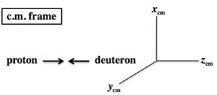
Figure 1: Proton-deuteron reactions in the center-of-momentum frame, where the deuteron moves in the $-z$ direction.

II.2 Rotations of deuteron polarizations
around transverse axes

The polarization vectors $\vec{E}_{+}$, $\vec{E}_{0}$, and $\vec{E}_{-}$ of Eq. (5) indicate the spin states $s_{z}=+1$, $0$, and $-1$ by taking the spin quantization axis in the $z$ direction. The $s_{z}=0$ state is given by the polarization vector $\vec{E}_{0}=(\,0,\,0,\,1\,)$. In the same way, the linear polarizations $\vec{E}_{x}=(\,1,\,0,\,0\,)$ and $\vec{E}_{y}=(\,1,\,0,\,0\,)$ correspond to the $s_{x}=0$ and $s_{y}=0$ states by taking the $x$ and $y$ axes, respectively, as the quantization axes, namely by rotating the $s_{z}=0$ state around the transverse axes with the angle $\pi/2$. If experimentalists can prepare such deuteron-target states, the proton-deuteron Drell-Yan cross-section difference $d\sigma(E_{x})-d\sigma(E_{y})$ can be measured as suggested theoretically in Ref. ks-gluon-trans-2019 . On the other hand, we explain in the following about the possibility of using the $\vec{E}_{+}$ ($s_{z}=1$) polarization by rotating the polarization around the transverse axes as shown in Fig. 2.

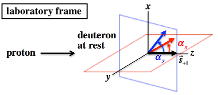
Figure 2: Proton-deuteron reactions in the laboratory frame, where the polarized deuteron is at rest with spin $\vec{s}_{+1}$. The spin vector $\vec{s}_{+1}$ is rotated with the angle $\alpha_{y}$ ($\alpha_{x}$) around the axis $y$ ($x$).

Since a finite polarization $S_{B,TT}^{\,xx}$ is needed for finding the gluon transversity $\Delta_{T}g(x)$ in Eq.(̇14), the deuteron state ($\vec{E}_{+}$) does not contribute for extracting $\Delta_{T}g(x)$ according to Eq. (11). Therefore, let us consider a rotation of the polarization vector $\vec{E}_{+}$ around the $y$ axis with the angle $\alpha_{y}$ in the laboratory frame with the deuteron at rest. Then, the polarization vector $\vec{E}_{+}$ becomes

$$\vec{E}_{\alpha_{y}}=\frac{1}{\sqrt{2}}\left(-\cos{\alpha_{y}},\,-i,\,\sin{\alpha_{y}}\right).$$ (24)

Using this polarization vector, we obtain the spin vector ${\mathbold S}$ and tensor ${\mathbold T}$ as

$$\!\!\!\!{\mathbold S}_{\alpha_{y}} =(\sin{\alpha_{y}},\,0,\,\cos{\alpha_{y}}),$$

$$\!\!\!\!{\mathbold T}_{\alpha_{y}} =\left(\begin{array}[]{ccc}\frac{1}{12}\left\{1-3\cos(2\alpha_{y})\right\}&0&\frac{1}{4}\sin(2\alpha_{y})\\[5.69046pt] 0&-\frac{1}{6}&0\\[5.69046pt] \frac{1}{4}\sin(2\alpha_{y})&0&\frac{1}{12}\left\{1+3\cos(2\alpha_{y})\right\}\end{array}\right).$$ (28)

These vector and tensor polarizations correspond to the parameter choice:

$$S_{T}^{x}=\sin{\alpha_{y}}, S_{T}^{y}=0, S_{L}=\cos{\alpha_{y}},$$

$$S_{LL}=\frac{1}{8}\left\{1+3\cos(2\alpha_{y})\right\}, S_{TT}^{xx}=\frac{1}{2}\sin^{2}{\alpha_{y}}, S_{TT}^{xy}=0,$$

$$S_{LT}^{x}=\frac{1}{2}\sin(2\alpha_{y}), S_{LT}^{y}=0.$$ (29)

If $\alpha_{y}=\pi/2$ is taken, the polarization vector becomes

$$\vec{E}_{\alpha_{y}=\pi/2} =\frac{1}{\sqrt{2}}\left(0,\,-i,\,1\right)=i\frac{1}{\sqrt{2}}\left(0,\,-1,\,-i\right)$$

$$\equiv i\vec{E}_{+/\hat{x}},$$ (30)

where $\vec{E}_{+/\hat{x}}$ is the polarization vector with the spin component $+1$ defined by taking the spin-quantization axis as $x$.

Next, if the rotation with the angle $\alpha_{x}$ is applied around the $x$ axis, the polarization vector $\vec{E}_{+}$ becomes

$$\vec{E}_{\alpha_{x}} =\frac{i}{\sqrt{2}}\left(i,\,-\cos{\alpha_{x}},\,-\sin{\alpha_{x}}\right).$$ (31)

In this case, the polarization parameters are given by

$$S_{T}^{x}=0, S_{T}^{y}=-\sin{\alpha_{x}}, S_{L}=\cos{\alpha_{x}},$$

$$S_{LL}=\frac{1}{8}\left\{1+3\cos(2\alpha_{x})\right\}, S_{TT}^{xx}=-\frac{1}{2}\sin^{2}{\alpha_{x}}, S_{TT}^{xy}=0,$$

$$S_{LT}^{x}=-\frac{1}{2}\sin(2\alpha_{x}), S_{LT}^{y}=0.$$ (32)

At $\alpha_{x}=-\pi/2$, it corresponds to the spin $+1$ state by taking the spin-quantization axis as $y$:

$$\vec{E}_{\alpha_{x}=-\pi/2} =-i\frac{1}{\sqrt{2}}\left(-i,\,0,\,-1\right)\equiv-i\vec{E}_{+/\hat{y}}.$$ (33)

In this way, rotating the deuteron spin around the transverse axes, we obtain a finite linear-polarization parameter $S_{TT}^{xx}$. Then, the gluon transversity can contribute to the gluon correlation function in Eq. (14) and then to the cross section. However, other spin parameters become finite according to Eqs. (29) and (32), the deuteron-polarization combination should be appropriately taken for extracting the gluon transversity distribution as the leading term. Such a combination will be shown later in Eq. (46).

III Polarized proton-deuteron Drell-Yan cross sections
for extracting gluon transversity

In the previous publication ks-gluon-trans-2019 , the proton-deuteron Drell-Yan cross sections were shown for the deuteron linear polarizations as $d\sigma(E_{x}\pm E_{y})$. However, since the linear polarizations are rarely used for the deuteron, we need to express them by the usual deuteron polarizations for actual experimental measurements. Let us consider the proton-deuteron Drell-Yan process with the unpolarized proton and the deuteron polarizations $\vec{E}_{\alpha_{y}}$ and $\vec{E}_{\alpha_{x}}$ or the deuteron spin vectors ${\mathbold S}_{\alpha_{y}}$, ${\mathbold S}_{\alpha_{x}}$ and tensors ${\mathbold T}_{\alpha_{y}}$, ${\mathbold T}_{\alpha_{x}}$.

In the unpolarized proton, there exists one type of twist-2 correlation-function terms, which correspond to the first terms of Eq. (12) and Eq. (14) of the deuteron case:

$$\Phi_{q/A}(x_{a}) =\frac{1}{2}\,\not{\bar{n}}\,f_{1,q/A}(x_{a}),$$

$$\Phi_{g/A}^{\,\alpha\beta}(x_{a}) =-\frac{1}{2}g_{T}^{\,\alpha\beta}\,f_{1,g/A}(x_{a}),$$ (34)

where the variable $x_{a}$ is the momentum fraction carried by a parton in the proton. The cross section of the proton-deuteron Drell-Yan process from the subprocess of $q\,(\bar{q})+g\to\gamma^{\ast}+q\,(\bar{q})$ typically contains the trace terms ks-gluon-trans-2019

$$\!\!\!\!\text{Tr}\left[(4\,\gamma\text{'s})\left\{\Phi_{q/A}(x_{a})+\Phi_{\bar{q}/A}(x_{a})\right\}\cdots(3\,\gamma\text{'s})\Phi_{g/B}^{\,\alpha\beta}(x_{b})\right],$$

$$\!\!\!\!\text{Tr}\left[(4\,\gamma\text{'s})\Phi_{g/A}^{\,\alpha\beta}(x_{a})\cdots(3\,\gamma\text{'s})\left\{\Phi_{q/B}(x_{b})+\Phi_{\bar{q}/B}(x_{b})\right\}\right].$$ (35)

In the same way, the subprocess $q+\bar{q}\to\gamma^{*}+g$ typically have the trace

$$\!\!\!\!\text{Tr}\left[(3\,\gamma\text{'s})\,\Phi_{q(\bar{q})/A}(x_{a})\cdots(3\,\gamma\text{'s})\,\Phi_{\bar{q}(q)/B}(x_{b})\right].$$ (36)

In Eq. (34), because there is one $\gamma$ in $\Phi_{q(\bar{q})/A}(x_{a})$ and no $\gamma$ in $\Phi_{g/A}^{\alpha\beta}(x_{a})$, possible terms in the deuteron correlation functions should contain no $\gamma$ in $\Phi_{g/B}^{\,\alpha\beta}(x_{b})$ and an odd number of $\gamma$ in $\Phi_{q(\bar{q})/B}(x_{b})$ so that the trace terms become finite.

Therefore, the relevant correlation-function terms, which contribute to the Drell-Yan cross section with the unpolarized proton, become

$$\!\!\Phi_{q/B}(x_{b}) =\frac{1}{2}\not{n}\,\bigg{[}f_{1,q/B}(x_{b})+\,S_{B,LL}\,f_{1LL,q/B}(x_{b})\bigg{]},$$

$$\!\!\Phi_{g/B}^{\,\alpha\beta}(x_{b}) =\frac{1}{2}\bigg{[}-g_{T}^{\,\alpha\beta}\,\left\{f_{1,g/B}(x_{b})+S_{B,LL}\,f_{1LL,g/B}(x_{b})\right\}$$

$$\ \ \ \ \ \ \ \ -S_{B,TT}^{\,\alpha\beta}\,\Delta_{T}g_{B}(x_{b})\,\bigg{]},$$ (37)

from Eqs. (12) and (14). Here, the lightlike vector $\bar{n}$ is replaced by $n$ as mentioned in the end of Sec. II.1. The $\alpha_{y}$ and $\alpha_{x}$ rotations around $y$ and $x$ in Fig. 2 indicate the parameter values as given in Eqs. (29) and (32):

$$\!\!\!\!\alpha_{y}\!:S_{B,LL}\!=\!\frac{1}{8}\left\{1\!+\!3\cos(2\alpha_{y})\right\}\!, S_{B,TT}^{xx}\!=\!\frac{1}{2}\sin^{2}{\alpha_{y}},$$

$$\!\!\!\!\alpha_{x}\!:S_{B,LL}\!=\!\frac{1}{8}\left\{1\!+\!3\cos(2\alpha_{x})\right\}\!, S_{B,TT}^{xx}\!=\!-\frac{1}{2}\sin^{2}{\alpha_{x}},$$ (38)

where the $\gamma_{5}\,\not{n}$ terms in the quark correlation function and the antisymmetric term $\epsilon_{T}^{\,\alpha\beta}$ in the gluon correlation function are also removed because their contributions vanish in the traces. The gluon transversity is denoted as $\Delta_{T}g_{B}=-h_{1TT,g/B}$ in Ref. ks-gluon-trans-2019 .

In the proton-deuteron Drell-Yan cross section, there are two types of cross sections as obvious from Eqs. (34), and (37):

$$\frac{d\sigma_{pd\to\mu^{+}\mu^{-}X}}{d\tau\,dq_{T}^{2}\,d\phi\,dy}=\frac{d\sigma_{0}(S_{B,LL})}{d\tau\,dq_{T}^{2}\,d\phi\,dy}+\frac{d\sigma_{\Delta_{T}g}(S_{B,TT}^{xx})}{d\tau\,dq_{T}^{2}\,d\phi\,dy}.$$ (39)

Here, the variable $\tau$ is defined by the dimuon-mass squared $M_{\mu\mu}^{2}$ and the center-of-mass-energy squared $s$ as

$$\!\!\!\tau=\frac{Q^{2}}{s},\ Q^{2}=(k_{1}+k_{2})^{2}=M_{\mu\mu}^{2},\ s=(p_{A}+p_{B})^{2},$$ (40)

where $k_{1}$ and $k_{2}$ are $\mu^{-}$ and $\mu^{+}$ momenta, and $p_{A}$ and $p_{B}$ are proton and deuteron momenta in the proton-deuteron Drell-Yan process, $p(p_{A})+d(p_{B})\to\mu^{-}(k_{1})+\mu^{+}(k_{2})+X$. The virtual photon momentum is denoted as $q$ ($=k_{1}+k_{2}$), and it is given as ks-gluon-trans-2019

$$q=(\,E,\,q_{T}\cos\phi,\,q_{T}\sin\phi,\,q_{L}),$$ (41)

by the transverse and longitudinal momenta $q_{T}$ ($=|\vec{q}\,|\sin\theta$) and $q_{L}$ ($=|\vec{q}\,|\cos\theta$) with the polar and azimuthal angles $\theta$ and $\phi$ in the c.m. frame. The dimuon rapidity $y$ is defined by

$$y=\frac{1}{2}\ln\frac{E+q_{L}}{E-q_{L}}=-\ln\left[\tan(\theta/2)\right],$$ (42)

in the c.m. frame. In Eq. (39), the first term $d\sigma_{0}(S_{B,LL})/(d\tau\,dq_{T}^{2}\,d\phi\,dy)$ is from the subprocess of the unpolarized PDFs in the proton with the unpolarized and tensor-polarized PDFs in the deuteron, and the second one $d\sigma_{\Delta_{T}g}(S_{B,TT}^{xx})/(d\tau\,dq_{T}^{2}\,d\phi\,dy)$ is from the gluon transversity distribution in the deuteron.

The first term of Eq. (39) is no more than the cross section of Eqs. (101) and (102) in Ref. ks-gluon-trans-2019 ; however, the unpolarized distributions should be replaced by unpolarized plus tensor-polarized one in the deuteron, $f_{1,X/B}(x_{b})+S_{B,LL}\,f_{1LL,X/B}(x_{b})$ with $X=q$, $\bar{q}$, or $g$, where $f_{1LL,X/B}(x_{b})$ is a tensor-polarized parton distribution, according to Eq. (37). The tensor-polarized PDF is related to the one $\delta_{T}f$ used in Ref. ks-2016 as $f_{1LL,X/B}(x_{b})=-(2/3)\delta_{T}f_{X/B}(x_{b})$ bacchetta-2000-PRD . However, the factor of 1/2 needs to be multiplied in Eqs.(101) and (102), where the combination $E_{x}+E_{y}$ was taken, and this factor appears in Eq. (43).

The second term corresponds to the cross section of Eq. (97) in Ref. ks-gluon-trans-2019 . However, here we take the specific polarization $S^{xx}_{B,TT}$ instead of the combination $E_{x}-E_{y}$ with $S^{xx}_{B,TT}=-1$ of Ref. ks-gluon-trans-2019 . Hence, Eq. (97) of Ref. ks-gluon-trans-2019 needs to be multiplied by $-(1/2)S^{xx}_{B,TT}$, as shown in Eq. (44).

The actual expression of the cross section is given for the first term as ks-gluon-trans-2019

$$\!\!\!\!\!\!\!\!\frac{d\sigma_{0}(S_{B,LL})}{d\tau\,dq_{T}^{2}\,d\phi\,dy}=\frac{\alpha^{2}\,\alpha_{s}\,C_{F}}{4\,\pi\,\tau\,s^{2}}\int_{\text{min}(x_{a})}^{1}dx_{a}\frac{1}{(x_{a}-x_{1})\,x_{a}^{2}\,x_{b}^{2}}$$

$$\!\!\!\!\!\!\!\!\!\times\sum_{q}e_{q}^{2}\,\bigg{[}\frac{4}{9}\left\{f_{1,q/A}(x_{a})\,f\,^{\prime}_{\!\!1,\bar{q}/B}(x_{b})+f_{1,\bar{q}/A}(x_{a})\,f\,^{\prime}_{\!\!1,q/B}(x_{b})\right\}\frac{2\tau\left\{\tau-(-2x_{a}x_{b}+x_{1}x_{b}+x_{2}x_{a})\right\}+x_{b}^{2}(x_{a}-x_{1})^{2}+x_{a}^{2}(x_{b}-x_{2})^{2}}{(x_{a}-x_{1})(x_{b}-x_{2})}$$

$$\ \ \ \ \ \ \ \ \ \ \ \ +\frac{1}{6}\left\{f_{1,q/A}(x_{a})+f_{1,\bar{q}/A}(x_{a})\right\}f\,^{\prime}_{\!\!1,g/B}(x_{b})\frac{2\tau(\tau-x_{1}x_{b})+x_{b}^{2}\left\{(x_{a}-x_{1})^{2}+x_{a}^{2}\right\}}{x_{b}(x_{a}-x_{1})}$$

$$\ \ \ \ \ \ \ \ \ \ \ \ +\frac{1}{6}\,f_{1,g/A}(x_{a})\left\{f\,^{\prime}_{\!\!1,q/B}(x_{b})+f\,^{\prime}_{\!\!1,\bar{q}/B}(x_{b})\right\}\frac{2\tau(\tau-x_{2}x_{a})+x_{a}^{2}\left\{(x_{b}-x_{2})^{2}+x_{b}^{2}\right\}}{x_{a}(x_{b}-x_{2})}\bigg{]},$$ (43)

where the parton distribution $f\,^{\prime}_{\!\!1,X/B}(x_{b})$ is defined as $f\,^{\prime}_{\!\!1,X/B}(x_{b})=f_{1,X/B}(x_{b})+S_{B,LL}\,f_{1LL,X/B}(x_{b})$. In the numerical analysis of Ref. ks-gluon-trans-2019 , the tensor-polarized PDFs $f_{1LL,X/B}(x_{b})$ are neglected because they are considered to be very small in comparison with the unpolarized PDFs. The variables $x_{1}$ and $x_{2}$ are given by the transverse mass $M_{T}=\sqrt{Q^{2}+\vec{q}_{T}^{\,\,2}}$, the rapidity $y$, and the c.m. energy squared $s$ as $x_{1}=M_{T}\,e^{\,y}/\sqrt{s}$ and $x_{2}=M_{T}\,e^{-y}/\sqrt{s}$. The momentum fraction $x_{b}$ and $\text{min}(x_{a})$ are expressed by these variables as $x_{b}=(x_{a}x_{2}-\tau)/(x_{a}-\tau)$ and $\text{min}(x_{a})=(x_{1}-\tau)/(1-x_{2})$. The second cross-section term is given by ks-gluon-trans-2019

$$\frac{d\sigma_{\Delta_{T}g}(S_{B,TT}^{xx})}{d\tau\,dq_{T}^{2}\,d\phi\,dy}=\frac{\alpha^{2}\,\alpha_{s}\,C_{F}\,q_{T}^{2}}{12\pi s^{3}}\,S_{B,TT}^{xx}\,\cos(2\phi)\int_{\text{min}(x_{a})}^{1} dx_{a}\frac{1}{(x_{a}x_{b})^{2}\,(x_{a}-x_{1})(\tau-x_{a}x_{2})^{2}}$$

$$\times\sum_{q}e_{q}^{2}\,x_{a}\left[\,f_{1,q/A}(x_{a})+f_{1,\bar{q}/A}(x_{a})\,\right]x_{b}\Delta_{T}g_{B}(x_{b}).$$ (44)

Now, let us consider the two rotations for the deuteron polarization in the laboratory frame with the deuteron at rest. One is to take the rotation angle $\alpha_{y}=\alpha$ around the $y$ axis, and the other is to take the rotation angle $\alpha_{x}=\alpha$ around the $x$ axis as shown in Fig. 2. Then, if we take the difference of the cross sections at the two angles, the first cross-section term $d\sigma_{0}(S_{LL})/(d\tau\,dq_{T}^{2}\,d\phi\,dy)$ drops and we obtain

$$\frac{d\sigma_{pd\to\mu^{+}\mu^{-}X}(\alpha_{y}=\alpha)}{d\tau\,dq_{T}^{2}\,d\phi\,dy} -\frac{d\sigma_{pd\to\mu^{+}\mu^{-}X}(\alpha_{x}=\alpha)}{d\tau\,dq_{T}^{2}\,d\phi\,dy}=\frac{\alpha^{2}\,\alpha_{s}\,C_{F}\,q_{T}^{2}}{12\pi s^{3}}\,\sin^{2}\alpha\,\cos(2\phi)$$

$$\!\!\!\!\!\!\!\!\!\!\!\!\!\!\times\int_{\text{min}(x_{a})}^{1}dx_{a}\frac{1}{(x_{a}x_{b})^{2}\,(x_{a}-x_{1})(\tau-x_{a}x_{2})^{2}}\sum_{q}e_{q}^{2}\,x_{a}\left[\,f_{1,q/A}(x_{a})+f_{1,\bar{q}/A}(x_{a})\,\right]x_{b}\Delta_{T}g_{B}(x_{b}).$$ (45)

On the other hand, their cross-section summation is given by

$$\frac{d\sigma_{pd\to\mu^{+}\mu^{-}X}(\alpha_{y}=\alpha)}{d\tau\,dq_{T}^{2}\,d\phi\,dy}+\frac{d\sigma_{pd\to\mu^{+}\mu^{-}X}(\alpha_{x}=\alpha)}{d\tau\,dq_{T}^{2}\,d\phi\,dy}=\frac{\alpha^{2}\,\alpha_{s}\,C_{F}}{2\,\pi\,\tau\,s^{2}}\int_{\text{min}(x_{a})}^{1}dx_{a}\frac{1}{(x_{a}-x_{1})\,x_{a}^{2}\,x_{b}^{2}}$$

$$\!\!\!\!\!\times\sum_{q}e_{q}^{2}\,\bigg{[}\frac{4}{9}\left\{f_{1,q/A}(x_{a})\,f\,^{\prime}_{\!\!1,\bar{q}/B}(x_{b})+f_{1,\bar{q}/A}(x_{a})\,f\,^{\prime}_{\!\!1,q/B}(x_{b})\right\}\frac{2\tau\left\{\tau-(-2x_{a}x_{b}+x_{1}x_{b}+x_{2}x_{a})\right\}+x_{b}^{2}(x_{a}-x_{1})^{2}+x_{a}^{2}(x_{b}-x_{2})^{2}}{(x_{a}-x_{1})(x_{b}-x_{2})}$$

$$\ \ \ \ \ \ \ \ \ \ \ \ +\frac{1}{6}\left\{f_{1,q/A}(x_{a})+f_{1,\bar{q}/A}(x_{a})\right\}f\,^{\prime}_{\!\!1,g/B}(x_{b})\frac{2\tau(\tau-x_{1}x_{b})+x_{b}^{2}\left\{(x_{a}-x_{1})^{2}+x_{a}^{2}\right\}}{x_{b}(x_{a}-x_{1})}$$

$$\ \ \ \ \ \ \ \ \ \ \ \ +\frac{1}{6}\,f_{1,g/A}(x_{a})\left\{f\,^{\prime}_{\!\!1,q/B}(x_{b})+f\,^{\prime}_{\!\!1,\bar{q}/B}(x_{b})\right\}\frac{2\tau(\tau-x_{2}x_{a})+x_{a}^{2}\left\{(x_{b}-x_{2})^{2}+x_{b}^{2}\right\}}{x_{a}(x_{b}-x_{2})}\bigg{]},$$ (46)

with the PDFs $f\,^{\prime}_{\!\!1,X/B}(x_{b})=f_{1,X/B}(x_{b})+\frac{1}{8}\left\{1\!+\!3\cos(2\alpha)\right\}\,f_{1LL,X/B}(x_{b})$.

Therefore, rotating the deuteron longitudinal polarization $\vec{s}_{+1}$ around the transverse coordinates $x$ and $y$ as shown in Fig. 2, we can measure the gluon transversity as the difference between the two cross sections $d\sigma(\alpha_{x}=\alpha)$ and $d\sigma(\alpha_{y}=\alpha)$, whereas their summation is given by the unpolarized and tensor-polarized PDFs of the deuteron. If $\alpha=\pi/2$ is taken, the gluon transversity distribution can be measured in the proton-deuteron Drell-Yan process with the deuteron polarizations along the two-transverse directions. In the same way, rotations of the polarization$\vec{E}_{-}$ or $s_{-1}$ can be used for investigating the gluon transversity distribution.

IV Summary

For finding the gluon transversity distribution of the deuteron in the proton-deuteron Drell-Yan process, the linear polarizations of the deuteron are needed theoretically as investigated in Ref. ks-gluon-trans-2019 . Since the linear polarizations are rarely used in handing the deuteron experimentally, we showed in this work that the Drell-Yan cross sections are expressed by the usual deuteron spin polarizations by rotating the spin vector around the two transverse axes. Then, we indicated that the difference of the two cross sections can be used for finding the gluon transversity distribution in the deuteron. With the transversely-polarized deuteron along two transverse directions, such a gluon transversity measurement is possible at hadron-accelerator facilities.

References

• (1) For review, see S. E. Kuhn, J.-P. Chen, and E. Leader, Prog. Part. Nucl. Phys. 63, 1 (2009); A. Deur, S. J. Brodsky, and G. F. de Teramond, Rep. Prog. Phys. 82, 076201 (2019), and references therein.
• (2) E. Leader and C. Lorce, Phys. Rep. 541, 163 (2014); M. Wakamatsu, Int. J. Mod. Phys. A 29, 1430012 (2014).
• (3) X. Ji, Phys. Rev. Lett. 110, 262002 (2013). For recent progress, see $e.g.$ T. Ishikawa et al., Phys. Rev. D 96, 094019 (2017); Huey-Wen Lin et al., Prog. Part. Nucl. Phys. 100, 107 (2018); Yu-Sheng Liu et al., Phys. Rev. D 101, 034020 (2020).
• (4) M. Diehl, Phys. Rep. 388, 41 (2003); S. Wallon, Doctoral school lecture notes on courses ED-107 and ED-517, Université Paris Sud (2014), unpublished.
• (5) K. Goeke, M. V. Polyakov, and M. Vanderhaeghen, Prog. Part. Nucl. Phys. 47, 401 (2001); X. Ji, Annu. Rev. Nucl. Part. Sci. 54, 413 (2004); A. V. Belitsky and A. V. Radyushkin, Phys. Rep. 418, 1 (2005); S. Boffi and B. Pasquini, Riv. Nuovo Cimento 30, 387 (2007); M. Diehl and P. Kroll, Eur. Phys. J. C 73, 2397 (2013); D. Mueller, Few Body Syst. 55, 317 (2014); K. Kumericki, S. Liuti, and H. Moutarde, Eur. Phys. J. A 52, 157 (2016); H. Moutarde, P. Sznajder, and J. Wagner, Eur. Phys. J. C 78, 890 (2018).
• (6) S. Kumano, Qin-Tao Song, and O. V. Teryaev, Phys. Rev. D 97, 014020 (2018).
• (7) U. D’Alesio and F. Murgia, Prog. Part. Nucl. Phys. 61, 394 (2008); V. Barone, F. Bradamante, and A. Martin, Prog. Part. Nucl. Phys. 65, 267 (2010); C. A. Aidala, S. D. Bass, D. Hasch, and G. K. Mallot, Rev. Mod. Phys. 85, 655 (2013); M. G. Perdekamp and F. Yuan, Annu. Rev. Nucl. Part. Sci. 65, 429 (2015).
• (8) V. Barone and R. G. Ratcliffe, Transverse Spin Physics (World Scientific, Singapore, 2003).
• (9) Z.-B. Kang, A. Prokudin, P. Sun, and F. Yuan, Phys. Rev. D 93, 014009 (2016); M. Radici and A. Bacchetta, Phys. Rev. Lett. 120, 192001 (2018); J. Cammarota et al., arXiv:2002.08384.
• (10) R. L. Jaffe and A. Manohar, Phys. Lett. B223, 218 (1989); J. P. Ma, C. Wang, and G. P. Zhang, arXiv:1306.6693 (unpublished).
• (11) M. Nzar and P. Hoodbhoy, Phys. Rev. D 45, 2264 (1992).
• (12) W. Detmold and P. E. Shanahan, Phys. Rev. D 94, 014507 (2016); 95, 079902 (2017).
• (13) F. Baldracchini, N. S. Craigie, V. Roberto, and M. Socolovsky, Fortsch. Phys. 30, 505 (1981); X. Artru and M. Mekhfi, Z. Phys. C 45, 669 (1990); S. Kumano and M. Miyama, Phys. Rev. D 56, R2504 (1997); A. Hayashigaki, Y. Kanazawa, and Y. Koike, Phys. Rev. D 56, 7350 (1997); W. Vogelsang, Phys. Rev. D 57, 1886 (1998); M. Hirai, S. Kumano, and M. Miyama, Comput. Phys. Commun. 111, 150 (1998).
• (14) W. Vogelsang, Acta Phys. Pol. B 29, 1189 (1998).
• (15) P. Hoodbhoy, R. L. Jaffe, and A. Manohar, Nucl. Phys. B312, 571 (1989); R. L. Jaffe and A. Manohar, Nucl. Phys. B321, 343 (1989); F. E. Close and S. Kumano, Phys. Rev. D 42, 2377 (1990); S. Hino and S. Kumano, Phys. Rev. D 59, 094026 (1999); 60, 054018 (1999); T.-Y. Kimura and S. Kumano, Phys. Rev. D 78, 117505 (2008); S. Kumano, Phys. Rev. D 82, 017501 (2010); J. Phys.: Conf. Series 543, 012001 (2014); G. A. Miller, Phys. Rev. C 89, 045203 (2014).
• (16) W. Cosyn, Yu-Bing Dong, S. Kumano, and M. Sargsian, Phys. Rev. D 95, 074036 (2017).
• (17) A. Airapetian et al. (HERMES Collaboration), Phys. Rev. Lett. 95, 242001 (2005).
• (18) Proposal to Jefferson Lab PAC-38, J.-P. Chen et al. (2011); K. Slifer, E. Long, and J. Maxwell, talks at the Workshop on Exploring QCD with light nuclei at EIC, Stony Brook, New York, USA, https://indico.bnl.gov/event/6799/ .
• (19) Fermilab E1039 experiment, Letter of Intent Report No. P1039 (2013), https://www.fnal.gov/directorate
/program_planning/June2013PACPublic/P-1039_LOI
_polarized_DY.pdf. For the ongoing Fermilab E-906
/SeaQuest experiment, see http://www.phy.anl.gov/mep
/drell-yan/.
• (20) S. Kumano and Qin-Tao Song, Phys. Rev. D 94, 054022 (2016).
• (21) A Letter of Intent to Jefferson Lab PAC 44, LOI12-16-006, M. Jones et al. (2016); R. L. Jaffe and A. Manohar, Phys. Lett. B 223, 218 (1989); E. Sather and C. Schmidt, Phys. Rev. D 42, 1424 (1990); J. P. Ma, C. Wang, and G. P. Zhang, arXiv:1306.6693 (unpublished).
• (22) J-PARC hadron project: https://j-parc.jp/Hadron/en/.
• (23) GSI-FAIR project: https://fair-center.eu/.
• (24) For the Spin Physics Detector (SPD) project at NICA, see http://spd.jinr.ru/.
• (25) D. Cebra, personal communications on the RHIC fixed-target project (2020).
• (26) S. Kumano and Qin-Tao Song, Phys. Rev. D 101, 054011 (2020).
• (27) M. Born and E. Wolf, Principles of optics (Cambridge University Press, Cambridge, 1999); J. D. Jackson, Classical Electrodynamics (John Wiley & Sons, Inc., New York, 1975).
• (28) E. Leader, Spin in Particle Physics (Cambridge University Press, Cambridge, 2001).
• (29) A. Bacchetta and P. J. Mulders, Phys. Rev. D 62, 114004 (2000).
• (30) T. van Daal, arXiv:1612.06585; arXiv:1812.07336, Ph. D. thesis, University of Groningen (2018).
• (31) D. Boer et al., J. High Energy Phys. 10, 013 (2016).