ML-AQP: Query-Driven Approximate Query Processing based on Machine Learning

Abstract.

As more and more organizations rely on data-driven decision making, large-scale analytics become increasingly important. However, an analyst is often stuck waiting for an exact result. As such, organizations turn to Cloud providers that have infrastructure for efficiently analyzing large quantities of data. But, with increasing costs, organizations have to optimize their usage. Having a cheap alternative that provides speed and efficiency will go a long way. Concretely, we offer a solution that can provide approximate answers to aggregate queries, relying on Machine Learning (ML), which is able to work alongside Cloud systems. Our developed lightweight ML-led system can be stored on an analyst’s local machine or deployed as a service to instantly answer analytic queries, having low response times and monetary/computational costs and energy footprint. To accomplish this we leverage the knowledge obtained by previously answered queries and build ML models that can estimate the result of new queries in an efficient and inexpensive manner. The capabilities of our system are demonstrated using extensive evaluation with both real and synthetic datasets/workloads and well known benchmarks.

1. Introduction

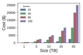
Figure 1. Costs associated with using cloud-managed databases (BigQuery). The x-axis is the amount of data used per query and the y-axis is the associated costs with the average number of queries daily.

With the rapid explosion of data volume and the adoption of data-driven decision making, organizations are struggling to analyze data efficiently and inexpensively. Hence, a lot of companies turn to Cloud providers that maintain large-scale data warehouses (sato2012bigquery, ; gupta2015amazon, ) able to store and process large quantities of data. But, the problem still remains: as multiple queries are issued by multiple analysts, clusters are often overburdened and costs rise significantly. For instance, looking at Figure 1, we can observe the exponential costs associated with an increasing data size. The associated cost (in y-axis) is obtained after multiplying the cost of scanning an amount of data (in x-axis) with varying number of queries shown as colored bars . Most importantly, during data analysis, it is of high importance to be able to extract information without significant delays so as to not break the interactivity constraint, which is set around 500ms (liu2014effects, ). This constraint supports that any answers returned over that limit can have negative effects on an analyst’s experience and productivity. Concretely, analysts often engage in what is called exploratory analysis (exploration, ) in order to better understand the data. Such analyses are an invariable step in the process of further constructing hypotheses or constructing and training predictive and inferential models to answer business questions. A key to these analyses is that an approximate answer to any query is often enough to move forward. As such, over the last few decades research has focused into systems that allow Approximate Query Processing (AQP)(garofalakis2001approximate, ; park2017databaseaqp, ; agarwal2013blinkdbaqp, ; kandula2016quickraqp, ) to facilitate the process of data analysis with this in mind. By trading off some of the accuracy they allow for order of magnitude speed-ups in execution.

Although AQP systems offer a straight-forward and efficient solution to the problem of efficiently processing queries, they come at a cost. They require large samples and would have to reside in the same Cloud system which makes them costly to maintain as every operation carries a cost. In addition, in cases where multiple analysts are using the Cloud system or AQP engine to process queries, they might be stuck waiting for their job to execute as multiple operations could be in the queue. Hence, what we propose is a complementary system to that of AQP engines addressing some of their shortcomings and better highlighting their strengths.

We envision a system that is computationally lightweight and can be stored in an analyst’s machine or in a central server, away from the main backend analytic system of choice. This allows for the exploratory process to be executed locally at the analyst’s machine, without overburdening the cloud system, thus, saving up resources (and money) to be used in cases where accurate answers are needed. From the cloud provider’s standpoint, our solution could act as a pseudo-caching mechanism to reduce load when it is necessary thus allowing for other operations to run.

What makes such a system possible, and the salient feature of our approach, is the availability of a number of previously executed queries (in log files). Leveraging previously executed queries allow for the creation of Machine Learning (ML) models that can estimate the results of new unseen queries. As exploratory analysis is often made up of operations that filter the data and then return descriptive statistics (aggregates) on the resulting subsets, we can construct ML models that predict such statistics. An ML model can effectively learn to associate the input parameter values of a query with the obtained result. Subsequent predictions can then be made in milliseconds, thus, fulfilling the interactivity constraint. In addition, most ML models are orders of magnitude lighter and can be stored on any device.

The desiderata are: Derived models are lightweight (in terms of memory footprint), easy to configure and fast to train, supporting error guarantees for their predictions, able to deal with updates to both query patterns and DB updates, able to handle all types of aggregate functions (AFs), and ensure high accuracy. Lastly, such mechanism does not require access to any of the data neither at training time, as is the case with current sampling-based and ML-based AQP approaches, nor at prediction time as what is being queried is the actual trained model. Concretely, our technical contributions are as follows:

• A flexible vectorized representation for (SQL) queries, to be used by ML models;

• The first AQP engine (ML-AQP) that mines query logs (query-driven) and develops ML models meeting all above desiderata;

• Up to 5 orders of magnitude greater efficiency than the state of the art sampling-based techniques;

• A new method for providing probabilistic error guarantees, based on Quantile Regression to complement approximate answers;

• Support for all AFs (including MIN/MAX which cannot be supported by current approaches);

• A comprehensive performance evaluation using synthetic and several real-world data sets and workloads which substantiate performance claims.

2. Preliminaries and Supported Queries

We abstract every (back-end) Cloud analytics system (both relational and non-relational) as a black box. Thus, essentially, queries are regarded as executing over sets of multi-dimensional points to which a number of operations are performed to return a result. Both non-relational and relational databases can be considered as large collections of attributes either grouped in a collection of normalized tables or being part of a single de-normalized data set. We can store our data in either of the two settings and the result of a query will still be the same. It is just the way of performing data manipulation and aggregation that differs. In the remainder of this section, we demonstrate how common operations in a relational schema can be performed using our proposed representation. This is without loss of generality to any kind of data-storage system and it is merely used as the abstraction should be familiar to the reader. Given the above, our first concern is to develop an appropriate representation for queries so that an ML model can associate the query representation with the query results and learn to predict answers for ’similar’ queries.

Definition 0.

(Data & Attributes) As we are unaware of the underlying data storage format, we adopt a generic assumption of all data being collections of attributes, where a dataset $\mathcal{B}$ is a collection of real-valued $d$-dimensional vectors $\mathbf{a}=(a_{1},\ldots,a_{d})$, such that $\mathcal{B}=\{\mathbf{a}\}_{i=1}^{n}$. The $\mathbf{a}$ vector holds values for $d$ attributes.

Definition 0.

(Aggregate Functions) Aggregate Functions (AF) are applied to the returned result-set and mapping a set of returned values to a scalar result $y\in\mathbb{R}$. An AF can be applied to a specific attribute; AFs commonly include functions such as COUNT, AVG, SUM. They are typically used in an SQL-style query along with various predicates and joins.

Definition 0.

(Predicates) Predicates are used to restrict the number of rows (data vectors) returned by a query. Predicates can be considered as a sequence of negations, conjunctions, and disjunctions ($\neg,\lor,\land$) over attributes with equality and/or inequality constraints ($\leq,\geq,=$). A well known predicate is the range-predicate. A range-predicate effectively restricts an attribute $a_{i}$ to be within a given range [$lb$, $ub$] with $a_{i}\geq lb\land a_{i}\leq ub$. To effectively model a sequence of predicates, we assign two meta-attributes for each attribute $a_{i}$ and consider every predicate as a range-predicate. The two meta-attributes are equal to the [$lb$, $ub$] of a range-predicate. For instance, without loss of generality, assume the three following predicates applied on a dataset with a single attribute $a_{1}$: (1) $a_{1}\geq lb$, (2) $a_{1}=c$, where $c$ is a numerical value, and (3) $a_{1}\geq lb\land a_{1}\leq ub$. We construct two meta-attributes for each case as follows: (1) $(a_{1,lb},-)$, where $-$ could be set to NULL and $a_{1,lb}$ is the supplied $lb$ value, (2) $(a_{1,c},a_{1,c})$, where $a_{1,c}=c$, and (3) $(a_{1,lb},a_{1,ub})$.

2.1. Transforming Aggregate Queries to Vectors

2.1.1. SPA Queries

We first consider Selection-Projection-Aggregate (SPA) queries, in which a single aggregate is the result of a query; that is made up of a single relation and multiple predicates. Given our definition of predicates, we obtain a meta-vector which is made up of all the constraints $\mathbf{m}=(a_{1,lb},a_{1,ub},\ldots,a_{d,lb},a_{d,ub})$ across all attributes. Hence, each SPA query can be represented by a meta-vector $\mathbf{m}\in\mathbb{R}^{2d}$. For all attributes that are part of the data set but not part of the query we leave the values of their associated meta-attributes as NULL. For instance, a simple SPA aggregate query is the following applied over a data set $\mathcal{B}$ with attributes $\mathbf{a}=(a_{1},a_{2},a_{3})$:

⬇

SELECT AF($a_{i}$)

FROM $\mathcal{B}$

WHERE $a_{1}\geq x_{1}\land a_{2}\leq x_{2}$

The meta-vector is $\mathbf{m}=(x_{1},\texttt{NULL},\texttt{NULL},x_{2},\texttt{NULL},\texttt{NULL})$.

2.1.2. SPJA Queries

To effectively model SPJA (Selection-Projection-Join-Aggregate) queries we first redefine what it means to join two or more tables together from a query representation perspective. We assume an architecture in schema design where, if multiple tables exist, then these tables are made up of a large fact table along with much smaller dimension tables. This is widely accepted in the literature (park2017databaseaqp, ; agarwal2013blinkdbaqp, ; hall2016trading, ). Specifically, in a designed AQP system by Google (hall2016trading, ) it is mentioned that all queried relations are pre-joined so that JOINs are not performed at query runtime. As a result, a data analyst simply queries the large fact table using equi-joins whenever they wish to project more attributes to the result set. Therefore, the dimensionality of the initial row (data vector) obtained from the fact table is simply increased. However, it is evident that the result set is still only affected by the predicates in the selection. Assuming these kind of JOINs and that the number of rows is not affected by the resulting JOIN our initial representation is appropriate without any changes.

2.1.3. GROUP-BY Queries

Supporting GROUP-BY queries is crucial for data analytics, as analysts often issue queries to explore differences between cohorts via grouping. A GROUP-BY query is an application of the same AF onto different sub-groups defined by an attribute. Hence, for an attribute $a_{i}$, we use a DISTINCT operator to identify the different groups and subsequently use the vectorization process of an SPA query on the individual groups. The result of the operator would be a set of group values $\mathcal{G}=(G_{1},\ldots,G_{k})$, which can be used as an equality predicate to construct $k$ different queries. An example of this is shown at Figure 2. An SQL query with a GROUP-BY clause is issued and the colored parts of this query are extracted. Suppose that the group-by attribute used is $a_{3}$, $a_{3}=g_{1}$. The predicate values $(x_{1},x_{2},x_{3},x_{4})$ and the extracted group values $(G_{1},\ldots,G_{k})$ are used to construct $k$ meta-vectors in which the values for $(a_{1,lb},a_{1,ub},a_{2,lb},a_{2,ub}$ contain the same values for all rows as the filter-predicates are applied for each group value $G_{1,i}$. The last two columns $a_{3,lb},a_{3,ub}$ are used to store the group values. Each one of those meta-vectors will become associated with the output of the corresponding AF.

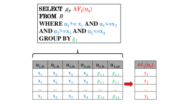
Figure 2. How to vectorize GROUP-BY queries.

This is similar to the formulation of Database Learning (park2017databaseaqp, ). However, we do not limit the number of generated queries to $1000$ as suggested by the formulation of (park2017databaseaqp, ). Hence, an arbitrarily large number of groups can be supported by our formulation.

2.1.4. Handling Categorical Attributes

Some attributes might hold categorical values instead of numerical. An accepted approach is to restrict the length of the categorical attributes to the currently longest of each categorical attribute (kraska2018case, ). Another option is to construct various dummy columns each one denoting a value included in the categorical attribute $a_{i}$(kuhn2013applied, ). Suppose $N$ distinct values for $a_{1}=(A_{1},\ldots,A_{N})$, then $N$ dummy columns are created, with its rows having a value of $\{0,1\}$, that being a mapping $A_{i}\to\{0,1\}$. However, the inherent problem with this option is the explosion in dimensionality of the query vector $\mathbf{m}$ as its dimensionalty now becomes $2d+N$. To this end, an effective encoding scheme can be an injective function, such as various hash functions, that provide an effective mapping from a categorical attribute to a real number, i.e., $\mathcal{A}\mapsto\mathbb{R}$. In our implementation for ML-AQP we use a combination of both. The first technique is used for attributes with low cardinality $<1000$. For tree-based ML algorithms, this has been shown to work best (kuhn2013applied, ). The latter technique is used for attributes with high cardinality $>1000$.

2.2. Overall Support for Queries & Limitations

Overall, with this representation we are able to support a large fraction of the aggregate queries commonly in an OLAP setting, from simple multi-predicate aggregation queries to queries that include JOINs and GROUP-BYs. We can provide support for foreign-key joins as this is the case for multiple AQP engines (park2017databaseaqp, ). Specifically our setting does not make any assumptions as to what type of aggregate functions are used. To ML-AQP the response variable is a scalar $y$, associated with a meta-vector $\mathbf{m}$. Subsequently it tries to identify patterns in $\mathbf{m}$ that would allow it to predict a future $y_{\text{new}}$ when given an $\mathbf{m}_{\text{new}}$. Therefore it is agnostic to the AFs used. This is in contrast to most sampling based AQP engines (agarwal2013blinkdbaqp, ) which restrict the number of aggregates supported. In addition, in the presence of textual filters (LIKE ’%product’) the same approach to other categorical attributes can be applied. Meaning that the pattern is considered as a string and encoded following the approach described at Section 2.1.4. For JOINs which do not simply extend the dimensionality but instead introduce less/more tuples in the result we do not explicitly represent them in the current meta-vector. As we described, usually such schema designs are avoided when conducting analyses over large amounts of data (hall2016trading, ). In addition, derived attributes for GROUP-BYs cannot be supported with our current formulation and instead such queries have to be partially executed to obtain the derived attributes.

3. System Architecture

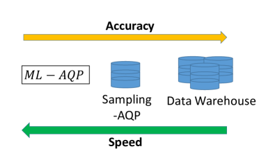
Figure 3. The ML-AQP within the complete data analytics stack. Starting from ML-AQP, analysts can choose a system going from left to right, if they require more accuracy. If speed is essential, they can choose from right to left.

Figure 3 shows holistically how ML-AQP complements the data analytics stack. Our system sits between cloud-based data warehouses and/or Sampling-based AQP engines. Using all three components (ML-AQP, sampling-based AQP engines, data warehouses), the analyst can choose which one to use based on their needs of efficiency and accuracy. A system could also make this choice based on the resources available. Hence, if a cloud system is experiencing heavy loads, it could direct queries to either the sampling-based AQP (S-AQP) engine or ML-AQP. A useful analogy is to think of each of the three components as the cache, RAM and Disk components of a computer. Caches and RAMs can often not hold the data required (hence the lack of accuracy), but the disk will always hold the true answer. However, this comes at a cost in efficiency. Therefore in our case, ML-AQP can act as the cache of the data analytics stack, sampling-based AQP engines as the RAM and finally cloud-based engines as the disk.

To better explain the overall architecture followed in ML-AQP, we explain each component as part of two distinct modes: (a) Training mode and (b) Prediction or Production mode. During Training mode, queries are either executed at the Data Warehouse or the S-AQP and become associated with their results. We can also utilise pre-computed queries stored at log files. ML-AQP leverages those queries to build training sets of query-result pairs for the ML models. Training these ML models transitions ML-AQP to the Prediction/Production mode to which queries are now being transformed into the described vectorial representation $\mathbf{m}$ and their results are estimated by ML models.

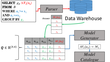
Figure 4. ML-AQP during Training

The complete flow and interaction of the components, is shown at Figure 4. Initially, at Training mode, each query is parsed, through the Parser, and the projected AFs are extracted $f_{1},\ldots,f_{n}$, along with the included predicates $p_{1},\ldots,p_{m}$ and any GROUP-BY attributes $g_{1},\ldots,g_{k}$. In the example at Figure 4, the extracted AF is $f_{1}=\texttt{AF}_{1}(a_{3})$, the resulting predicates are $p_{1}=(a_{1}\geq x_{1})$ and $p_{2}=(a_{1}\leq x_{2})$ and the GROUP-BY attribute is $g_{1}$. For the predicates, we construct an $\mathbf{m}\in\mathbb{R}^{2d}$ meta-vector, where $d$ is total number of attributes in a data set. Each meta-vector is associated with a number of results $y_{1},\ldots,y_{n}$, obtained from the executed AFs. If no GROUP-BY attributes are included then we call this a single query $\mathbf{q}=(\mathbf{m},\mathbf{y}),\mathbf{q}\in\mathbb{R}^{2d+n}$. For any, GROUP-BY attribute $g_{i}$ a SELECT-DISTINCT query is executed and its result is cached in GROUP-BY catalogue $D$. The catalogue $D$ is a mapping from the GROUP-BY attribute $g_{i}$ to its set of distinct values $D:g_{i}\to\mathcal{G}_{g_{i}}$. Caching its result allows their reuse during Prediction/Production mode. For any GROUP-BY attributes that are frequently used together such as $(g_{i},g_{j})$ we also cache their set of distinct values. Given the values returned for $g_{i}$, $\mathcal{G}_{g^{(i)}}=\{G_{g_{i},1},\ldots,G_{g_{i},|G_{g_{i}}|}\}$, we construct multiple single-queries which have different results for $y_{1},\ldots,y_{k}$ as they correspond to different groups. Hence, in the case of GROUP-BY queries, a single query has a matrix representation for its meta-vectors and their associated results $\mathbf{Q}=(\mathbf{M},\mathbf{Y}),\mathbf{Q}\in\mathbb{R}^{(|G_{g_{(i)}}|)\times(2d+n)}$, this result is shown at Figure 4. The same procedure occurs for each executed query, which results in the collection of possibly sparse vectors (as not each attribute is often included in the predicates or the GROUP-BY clause). Because of this, we store all of the processed queries in a sparse matrix to save space. Once we finish parsing and constructing the representation for each query in our training set, we use the Model Generator to construct/train models $\mathcal{M}_{i},\mathcal{M}_{n}$ for each AF encountered and an association is created $\texttt{AF}_{1}(a_{3})\to\mathcal{M}_{1}$. The models are then serialized and stored in a Model Catalogue.

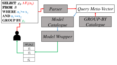
Figure 5. ML-AQP during Production/Prediction

A similar process occurs during the Prediction/Production mode when a new (SQL) query is issued at the ML-AQP. The complete flow of interactions between sub-components is shown at Figure 5. During initialization of the ML-AQP, both the GROUP-BY catalogue and Model Catalogue are loaded in memory. Consider the same query used as an example at Figure 4, but this time the query is not sent for execution but instead ML-AQP is asked to predict its answer. Again the Parser is used to extract the same elements (predicates, AFs, GROUP-BY attributes). A vectorized representation of the query is constructed at Query Meta-Vector. If a GROUP-BY statement exists, the resulting meta-vector is a matrix $\mathbf{M}$ and the values for $g_{i},\ldots,g_{k}$ are obtained from the GROUP-BY catalogue storing different $\mathcal{G}_{g_{i}}$. If the group-by attributes have been cached together then that result is fetched from the catalogue. The necessary AFs to be estimated are identified and their models are fetched from Model Catalogue. The Model Wrapper is used to query the model and estimate the results given the meta-vector $\mathbf{m}$. The result(s) are then returned to the user in an efficient manner as no data are accessed and the only overhead is the inference time of a model.

4. Machine Learning Specifics

Each query result $y$ from the training pair $(\mathbf{m},y)$ derives from an unknown true function $f(\cdot)$. Such function produces answers w.r.t an unknown conditional distribution $p(y|\mathbf{m})$. Our aim is to approximate the true functions $f$ for each aggregate function e.g., COUNT, AVG, MIN, MAX, SUM, etc. Supervised ML algorithms are adopted to minimize the expected prediction loss between the actual answer $y=f(\mathbf{m})$ from the true function $f(\cdot)$ and the predicted $\hat{y}$ from an approximated function $\hat{f}(\cdot)$ generated by the ML model:

(1) $$\min_{f}\mathbb{E}[\mathcal{L}(f(\mathbf{m}),\hat{f}(\mathbf{m}))]$$

The loss $\mathcal{L}(\cdot,\cdot)$ can be usually measured using absolute or squared loss functions: $\mathcal{L}=|f(\mathbf{m})-\hat{f}(\mathbf{m})|\mbox{ or }\mathcal{L}=(f(\mathbf{m})-\hat{f}(\mathbf{m}))^{2}.$ Supervised learning algorithms minimize the expected prediction loss using training examples, which they use to learn the true function $f$. Such training examples are the query-answer pairs in $\mathcal{C}$, which are drawn from $P(y|\mathbf{m})$ and are thus a sample of this distribution. Hence, by minimizing the sample error we expect to obtain good estimation over any unseen query. Our objective over the sample shown at Eq.2 is to minimize the Mean Squared Error (MSE) as it is commonly used in regression algorithms (friedman2001elements, ):

(2) $$\frac{1}{N}\sum_{i}^{N}(y_{i}-\hat{f}(\mathbf{m}_{i}))^{2}.$$

Note, various supervised learning algorithms minimize a variant of the objective in (2) including regularization parameters as a technique to avoid overfitting (friedman2001elements, ).

Going back to our use case, we obtain a set of queries and their responses $\mathcal{C}=\{(\mathbf{m},\mathbf{y})\},\mathbf{m}\in\mathbb{R}^{2d},\mathbf{y}\in\mathbb{R}^{n}$. We treat queries that have a matrix representation $\mathbf{Q}$ as collections of single queries. This makes sense as essentially each row in $\mathbf{Q}$ corresponds to a single query if instead of the GROUP-BY attribute a single predicate existed restricting $g_{i}$ to a single value. The task is to train ML models $\mathcal{M}_{i},\ldots,\mathcal{M}_{n}$ that would produce regression functions $\hat{f}_{i},\ldots,\hat{f}_{n}$ that minimize MSE. Multiple such regression algorithms exist and to make the right choice we have to consider some of the properties of the problem at hand.

4.1. Choice of Machine Learning Models

A primary concern is that the produced training set $\mathcal{C}$ is inherently sparse as both the parameter vector $\mathbf{m}$ and response vector $\mathbf{y}$ contain NULLs (which can be represented as zeroes in linear algebra) for (a) attributes that do not have any predicates set on them and, hence, $a_{i,lb},a_{i,ub}$ would be NULL or zero, (b) queries that do not include an AF producing a response variable $y_{i}$ would also have NULL values for $y_{i}$. For instance, in a dense matrix representation consider two queries calling different AFs; $\texttt{AF}_{1}$ and $\texttt{AF}_{2}$, to represent as a matrix we have to set up two columns $\texttt{AF}_{1}$ and $\texttt{AF}_{2}$ with the first row (for the first query) having a NULL value for $\texttt{AF}_{2}$ and the second row having NULL for $\texttt{AF}_{1}$. To alleviate the NULL response problem we partition the dataset per response/AF such that queries that refer to the same AF are grouped together. However, the input is still sparse. Hence we need algorithms that are able to handle such problems effectively.

Linear models can often be trained in an online manner using SGD (bottou2012stochastic, ), which makes them very efficient. However, they result in simple models which cannot adequately model non-linear relationships without introducing more polynomial terms. Models such as Ridge and Lasso (friedman2001elements, ) regression are interesting variants that include regularization to handle the increased dimensionality of our input. However, we have found that these algorithms do not perform well for our problem. We have also considered the use of Deep Learning, however the models become unnecessarily complex, hard to interpret, expensive to train, difficult to tune and have high inference times (kraska2018case, ) which could increase the latency of estimating the response of an issued query. hence, they violate the desiderata set earlier.

In light of the above arguments, we have made the choice of using Gradient Boosting Machines (friedman2001greedy, ) (GBM) using efficient-parallel implementations called XGBoost(chen2016xgboost, ) and LightGBM(ke2017lightgbm, ). A GBM iteratively fits decision trees, at first trying to approximate the response variable and then making this approximation more fine-grained by combining decision trees trained on the negative gradient of the response variable and the produced predictions by the last decision tree. In addition, the highly scalable implementation of GBM by XGBoost and LightGBM allows handling large, high dimensional and sparse input.

4.2. Error Guarantees

A highly desirable feature of any AQP engine is its ability to offer error guarantees to the user, regarding its approximated answers. For sampling-based AQP engines, providing such guarantees is relatively straightforward: Using subsampling/bootstraping methods, confidence intervals ($[low,high]$) can be derived, associated with certain confidence levels ($l\%$), indicating that the sampled-population statistic of interest (say, the mean) will fall within the $[low,high]$ range with probability $l\%$ (park2018verdictdbaqp, ; kandula2016quickraqp, ; agarwal2013blinkdbaqp, ; olma2019tasteraqp, ). However, this is not appropriate for AQP engines which, instead of inferring population statistics of a sampled population, employ predictive-ML-based models for predicting answers to future questions.

Therefore, as ML-AQP relies on predictive/regression ML models, the produced $\hat{y}$ is not an estimator of a population parameter, but a prediction of the answer for a future query (vector $\mathbf{m}$). Hence, we start off our discussion with a naive solution of offering some kind of error estimation for aggregate answers. All ML models are assessed and minimize what is known as the Expected Prediction Error (EPE). This is measured by the loss stated at (2). During training mode, this is an over-optimistic estimate of the generalizability error that the specific ML model is associated with. The generalizability error is an estimate of the error associated with any future estimations. However, because ML models are trained on the set used for measuring EPE, they tend to produce inaccurate estimates. Hence, we use cross-validation (friedman2001elements, ) that measures the EPE on out-of-sample examples that the model did not use during training. Although, techniques such as Leave-One-Out (LOO) and K-Fold (friedman2001elements, ) produce good estimates for the EPE, this is not probabilistically guaranteed. In addition, the EPE is static across the input space. This means that, even though an ML model might have learned to predict the answers of certain queries with error $\epsilon_{1}$ and some others with error $\epsilon_{2}$, and $\epsilon_{1}\ll\epsilon_{2}$, both sets of queries will have the same EPE associated with them. We find this assumption of a static EPE as undesirable.

Instead of the estimate for EPE, we can use Prediction Intervals: Unlike confidence intervals, which are used to provide an interval for a population parameter, prediction intervals are used to provide intervals that contain the $true$ ($not\ predicted$) value of an aggregate result $y_{n+1}$ of a future query (vector $\mathbf{m_{n+1}}$)). If we knew that the distribution of $y$ is Normal and that any $y$ is independent, prediction intervals could be produced similarly to confidence intervals. Using the sample of $y$ given from the training examples $(y_{1},\ldots,y_{n})$, we compute the interval: $\overline{y}\pm t_{a}s_{n}\sqrt{1+\frac{1}{n}}$, where $t_{a}$ is the $100(1-\frac{a}{2})^{\text{th}}$ percentile of the $t$-distribution, with $\alpha\in(0,1)$ and commonly set to $\alpha=0.01$ or $\alpha=0.05$, $s_{n}$ is the sample variance of the response variable $y$ and $1-\alpha$ is the coverage of the prediction interval. However, we do not wish to make any parametric assumption about the distribution of $y$. Hence, we resort to other methods outlined below.

As mentioned, bootstrap (bootstrap, ), is a prominent method which makes no parametric assumptions about the distribution of $y$. This is used among sampling based AQP engines as well (zeng2014analytical, ; agarwal2014knowing, ). In a sampling-based AQP engine, the bootstrap method is adopted to re-sample the underlying data set $b$ times (where $b$ is usually over $>100$) and produce a distribution of estimates for $y$, $\hat{y}_{i,1},\ldots,\hat{y}_{i,b}$. Let $y_{i,0}$ be the original estimate, with the estimates provided by the bootstrap samples, we then compute the residuals $y_{i,0}-\hat{y}_{i,1},\ldots,y_{i,0}-\hat{y}_{i,b}$. Using the empirical distribution of residuals, we then compute quantiles, which can be used to produce a confidence interval $[\hat{y}_{i,0}-t_{1-{a/2}},\hat{y}_{i,0}+t_{a/2}]$. Theoretically, ML-AQP could also use the bootstrap method, re-sampling the training dataset $b$ times and constructing $b$ ML models $M_{i},\ldots,M_{b}$. This would yield $b$ estimates for $y$, $\{\hat{y}\}_{i=1}^{b}=\{\hat{f}_{i}(\mathbf{m})\}_{i=1}^{b}$ and can similarly produce confidence intervals. However, this methodology would incur the costs of training, maintaining, and predicting the estimates from $b+1$ (if we count the initial model providing the prediction) different ML models. Multiply that by the number of different AFs that need to be learned and the overhead cost of this approach quickly becomes huge.

More recent developments in ML literature focus on building predictive intervals by making use of conformal inference (shafer2008tutorialconformal, ; lei2018distributionconformal, ; papadopoulos2011regressionconformal, ). This technique relies on building a non-conformity measure which estimates the difference of two examples i.e., $\mathbf{m}_{i}$ and $\mathbf{m}_{j}$. This could be defined as the $L_{p}$ norm (i.e $p=2$) of the examples $\lVert\mathbf{m}_{i}-\mathbf{m}_{j}\rVert_{2}^{2}$. But finding the right non-conformity measure in our case is non-trivial as the input vectors are high-dimensional and sparse. Distance in this case becomes meaningless (aggarwal2001surprising, ) and the choice of a valid $p$-norm is beyond the scope of this work. In addition, these techniques scan the complete set of previous training examples to find similar and dissimilar examples. Thus, all previous queries have to remain stored. This is undesirable, as we would like to discard all of the queries and only deploy models for ML-AQP.

Therefore, our choice is to employ Quantile Regression (QR) (koenker2001quantile, ). While typical regression models minimize the EPE and focus on estimating the conditional expectation $\mathbb{E}[y|\mathbf{m}]$, QR tries to estimate the $t^{\text{th}}$ conditional quantile $Q_{y|\mathbf{m}}(t)$. Multiple ML algorithms have been proposed to estimate conditional quantiles (steinwart2011estimating, ; meinshausen2006quantile, ; takeuchi2006nonparametric, ). Formally, given a conditional distribution function for $y$,

(3) $$F_{y|\mathbf{m}}=\mathbb{P}\{Y\leq y|\mathbf{m}\},$$

we define the $t^{\text{th}}$ conditional quantile function as:

(4) $$q_{t}(\mathbf{m})=\inf\{y\in\mathbb{R}:F_{y|\mathbf{m}}>t\}$$

Where $\inf$ is the infimum, which points to $y$ that is less than or equal to all the elements in the defined set. Given the conditional quantile function defined in (4), we construct prediction intervals using $[q_{t/2},q_{1-t/2}]$. This defines the lower and upper bounds of the estimated value for $y$ with coverage probability of $100(1-t)\%$. As stated, earlier regression algorithms estimate the conditional expectation of $y$, $\mathbb{E}[y|\mathbf{m}]$ by minimizing EPE. In the same manner, quantile regression algorithms estimate the conditional $t^{\text{th}}$ quantile $Q_{y|\mathbf{m}}(t)$ by minimizing what is known as ”pinball loss”(koenker2001quantile, ) :

(5) $$\rho_{t}(y,\hat{y})=\begin{cases}t(y-\hat{y}),\quad\text{if}\quad y-\hat{y}>0\\ (1-t)(\hat{y}-y),\quad\text{otherwise}\end{cases}$$

Suppose we have trained two different quantile regression functions $\hat{q}_{t/2}:\mathbf{m}\in\mathbb{R}^{2d}\to Q_{y|\mathbf{m}}(t/2)\in\mathbb{R}$ and $\hat{q}_{1-t/2}:\mathbf{m}\in\mathbb{R}^{2d}\to Q_{y|\mathbf{m}}(1-t/2)\in\mathbb{R}$. Then, a prediction interval for each new query is estimated as: $[\hat{q}_{t/2}(\mathbf{m}_{\text{new}}),\hat{q}_{1-t/2}(\mathbf{m}_{\text{new}})]$ with coverage probability $100(1-t)\%$.

Therefore, ML-AQP provides error guarantees using QR and the statistical tools of prediction intervals and coverage. Specifically, ML-AQP produces a prediction interval $[low,high]$ and a coverage level $l\%$ and guarantees that the $true$ answer to a future query will fall within $[low,high]$ with probability $l\%$. LightGBM (ke2017lightgbm, ) offers support for QR and we are also looking into incorporating (romano2019conformalized, ) to support stricter guarantees.

5. Updates

As ML-AQP is deployed, over the course of time there might be significant data updates or drastic workload shifts that invalidate the patterns learned by the models so far. In general new query patterns or new data might not cause the accuracy of ML-AQP to deteriorate as it is still able to generalize. Formally, we require workload/data updates to be significant so that the distributions at times $t$ and $t+1$ are no longer the same, meaning that the condition, $p_{t}(y)\neq p_{t+1}(y)$, holds for data updates and $p_{t}(\mathbf{m})\neq p_{t+1}(\mathbf{m})$ for workload shifts. Although insertions/updates/deletions could be expected to be frequent, $p(y)$ might not change. Therefore, the key observation is that we do not need to track changes in the data space but instead need to monitor for changes in $p(y)$. To tackle both workload/data shifts we could naively retrain the models at fixed time intervals to be sure that the most updated queries and data are used. Over, 1M+ queries are executed daily in large deployments (kandula2016quickraqp, ); thus, it is easy/fast to find new queries executed on fresh data. However, we provide two alternative methods and in the next paragraphs we first address data updates and then workload shifts.

As shown previously, our solution is query-driven and does not access data at any time. Therefore, to detect changes in the data/workload, we monitor queries that are successively executed by the data warehouse $(\mathbf{q}_{t},\ldots)$. To detect changes to the aggregates distribution $p(y)$ we employ the two-sample Kolmogorov-Smirnov (KS) test. The KS test output statistic is $D=\sup_{y}|F_{1}(y)-F_{2}(y)|$, where $F_{1}$ is the empirical CDF (ECDF) at time $t$ of answers $\mathcal{Y}_{1:t}$ of all queries that were used to train a model and $F_{2}$ is the ECDF of $\mathcal{Y}_{t+1:}$ from monitored queries executed against the data warehouse. The KS test, evaluates the hypothesis that the two sets of answers come from the same distribution. The hypothesis is rejected at a significance level $\alpha$ if $D>c(a)\sqrt{\frac{n+m}{nm}}$, where $c(a)=\sqrt{-\frac{1}{2}+\ln{\frac{\alpha}{2}}}$ and $n=|\mathcal{Y}_{1:t}|$, $m=|\mathcal{Y}_{t+1:}|$ . If the hypothesis is rejected then the distribution has shifted and the model associated with the aggregate needs to be retrained. Retraining a model because of a distribution shift does not impose a large overhead as the cost of training the models is minimal, (as shown in Section 6.4). We are also considering other solutions such as data augmentation (tanner1987calculation, ) to augment the existing set of queries and allow our models to generalize to possible data updates without retraining.

We also need to address the case of a workload shift and employ a similar detection test. The workload is characterised by the query vectors $\mathbf{m}\in\mathbb{R}^{2d}$ and the KS test cannot be applied as their distribution $p(\mathbf{m})$ is multivariate. In this case we can apply Chebyshev’s inequality which states that; given a random variable $X$ and its expected value $\mu$ then the probability of obtaining a sample point greater than $k$ standard deviations from the mean is $\leq\frac{1}{k^{2}}$, formally $Pr(|X-\mu|\geq k\sigma)\leq\frac{1}{k^{2}}$. This is clearly defined for a scalar value $X$ and we need the multivariate version of this as we have vectors $\mathbf{m}\in\mathbb{R}^{2d}$. For the multivariate case we can express the above as $Pr(\sqrt{(\mathbf{m}-\mathbf{\mu})^{T}\Sigma^{-1}(\mathbf{m}-\mathbf{\mu})}\geq k)\leq\frac{N}{k^{2}}$, where $\Sigma$ is the covariance matrix and $N=Tr[\Sigma^{-1}\Sigma]$. Hence, as queries are being monitored we can examine the inequality and trigger an alarm to retrain the models if the inequality is violated, meaning that if $Pr(\sqrt{(\mathbf{m}-\mathbf{\mu})^{T}\Sigma^{-1}(\mathbf{m}-\mathbf{\mu})}\geq k)\geq\frac{N}{k^{2}}$ then we need to retrain the models because of a workload shift.

6. Evaluation

6.1. Experimental Setup

Datasets & Workloads. For our experiments we used the following data sets and workloads:

1. TPC-H(tpch, ): This is the standard TPC-H benchmark.

2. Instacart(instacart, ): This is a data set of an online store. A database was created using the csv files which follows the setup of VerdictDB. (park2018verdictdbaqp, ).

3. Crimes(crimesdata, ): This is a real data set of crimes reported in the city of Chicago. A workload for this data set was obtained from (crimes_workload, ) which models a number of range-queries with multiple AFs. Their predicates are sampled from a number of random distributions to simulate various analysts executing queries at different subspaces of the data set.

4. Sensors(sensors, ): Is a data set comprised of a number of sensor readings including voltage, humidity temperature etc with a temporal dimension. A synthetic workload was created restricting the temporal dimension and extracting the MIN(temperature) and MAX(humidity).

Training ML-AQP. ML-AQP has a Training phase, much like sampling based AQP engines that need to create samples before being able to operate. For all workloads, we generate queries and train the models on $70\%$ of the complete workload. We then conduct the experiments and take measurements on the rest $30\%$. This is standard practise in the ML literature. For Instacart, we use a similar format of queries as VerdictDB (verdict-instacart, ). However, to facilitate learning we vary the predicate values. For all queries containing predicate values, we generate queries from the same template with values sampled from a normal distribution $\mathcal{N}(\mu,\sigma)$, where $(\mu,\sigma)$ is the average and standard deviation of the corresponding attribute, respectively. If the attribute contains a categorical value, the generated queries contain a value selected uniformly at random. The total number of training queries generated were $10^{4}$ and $3.3\cdot 10^{3}$ for testing. Some queries contained no predicates, in these cases no additional queries were generated. The number of queries obtained is not large as typically there are millions of queries being executed on a daily basis in production environments (kandula2016quickraqp, ).

For TPC-H, we use a subset of the queries contained in the benchmark as we are still making progress on our Parser. We generate $100$ queries for each of the queries used. A model is trained for each distinct AF. For Instacart, three different models are generated as three distinct AFs are used in this workload. For TPC-H, $12$ different models were generated. For Crimes and Sensors. we generate a model per AF tested.

6.2. Performance

We first examine the performance of ML-AQP and demonstrate the speedup gains over a popular database PostgreSQL. We compare the results using a sampling based AQP engine, VerdictDB (park2018verdictdbaqp, ). Let $t_{b}$ be the response time for PostgreSQL and $t_{m}$, $t_{v}$ the response times for ML-AQP and VerdictDB then speedup is measured by $\frac{t_{b}}{t_{m}}$ and $\frac{t_{b}}{t_{v}}$, respectively. For this experiment, we use TPC-H with 1GB and Instacart with its main fact tables (order_products, orders) containing $~{}3$M and $~{}30$M rows. For TPC-H, we use a subset of all the template queries and for Instacart, we use the same format of queries as used in the evaluation of VerdictDB(verdict-instacart, ). For VerdictDB, uniform samples were created for large fact tables at $1\%$/$10\%$ ratio. This experiment ran on a single machine with an Intel(R) Core(TM) i7-6700 CPU @3.40GHz, 16GB RAM and 1TB HDD.

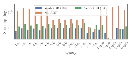
Figure 6. Speedups offered by ML-AQP compared to VerdictDB

The results are shown at Figure 6. We can instantly notice that the speedup differences are huge (notice the log-scale on y-axis). Even though we are using relatively small datasets, VerdictDB, understandably, cannot offer the same speedup as ML-AQP. The minimum/maximum speedup gained by ML-AQP is at $7\times$/$7200\times$,for VerdictDB $1\%$ $0.59\times$/$43\times$ (as we suspect that some of the computation is offloaded to the main engine) and for VerdictDB $10\%$ $3\times$/$11\times$. This stems from the fact that ML-AQP is only performing inferences at Prediction mode using trained models. It does not need to scan any of the data at any time. To be more specific, Table 1 shows the mean response time along with the standard deviation and $95^{\text{th}}$ percentile for all queries across the four different systems. As it is evident, even at the $95^{\text{th}}$ percentile the response times for ML-AQP are no greater than $120$ milliseconds, satisfying the interactivity constraint set at $500$ms (liu2014effects, ).

System	Time (sec)	$95^{\text{th}}$ percentile (sec)
PostgreSQL	$1.62\pm 1.21$	$4.01$
VerdictDB (10%)	$0.28\pm 0.41$	$0.79$
VerdictDB (1%)	$0.14\pm 0.3$	$0.43$
ML-AQP	$0.05\pm 0.16$	$0.12$

Table 1. Performance over all queries across systems

Even for queries with relatively large GROUP-BYs the speedup is at $20x$. By default GROUP-BYs are a bottleneck in our case as multiple queries have to be executed for each distinct value of the attribute used in the GROUP-BY clause. For instance, query $14$-ic has approximately $50$K distinct values. In this experiment its values were cached as this would have been the default behavior. This is due to similar queries with the same GROUP-BY attributes being executed during Training mode. When caching the values, query $14-ic$ takes $0.67$ seconds to execute and $0.7$ seconds when it does not cache the GROUP-BY values. We can see minor impact, with an overhead attributed to the execution of the SELECT DISTINCT query at $0.3$ seconds. We can still get $7x$ better response times than PostgreSQL, where as VerdictDB ($1\%$/$10\%$) is at $24x/3x$ for this particular query. Although a larger speed-up is observed, for VerdictDB($1\%$) we will notice that accuracy using $1\%$ sampling ratio deteriorates with large errors in the individual groups.

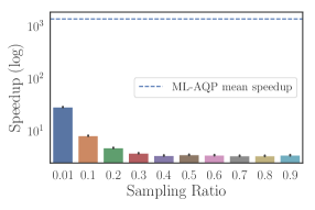
Figure 7. VerdictDB speedup for an increasing sampling ratio.

At Figure 7 we examine how the speed-up offered by sampling based and in general data-driven AQP solutions diminishes as the sampling ratio is increased. For point of reference we also provide the average speedup offered by ML-AQP which is not constrained by a sampling ratio as it uses no data.

6.3. Performance at the Cloud

Our solution is designed to alleviate the monetary, computational, storage costs in large deployments usually in the cloud. We first examine how the computational cost can be mediated using our solution. For this experiment, we use AWS Redshift, with 2 dc2.large compute nodes and $1$ master node each at 16GB memory with 160GB SSD. We use a $100x$ scaled version of the Instacart dataset. The total storage footprint of this data set is $~{}100$GB with the main fact tables (order_products, orders) containing $4.2$ billion and $0.5$ billion rows respectively. We execute the same Instacart queries (verdict-instacart, ) and we set a timeout value at $5$(mins). After this, we abort the execution of the query. For VerdictDB we uniformly sample the same fact tables at $10\%$ ratio. In this experiment, we expect the results for VerdictDB to deteriorate. On the other hand ML-AQP is constant in its performance as it is unaffected by data size. It is important to recall that the deployment of ML-AQP can happen in two ways: (i) All the models and required modules for ML-AQP can be distributed to all the analysts’ machines and be loaded in memory during analysis (later experiments will showcase that the small storage footprint of ML-AQP permits this solution); (ii) All models can be deployed at a server and be used as a service. This would have significantly lower costs than executing queries using Redshift. However, it might have more overhead as the predictions have to be transferred to the analysts machine over the network. We further examine the performance benefits of both solutions.

The results of this experiment are shown at Figure 8. There are two different deployments for ML-AQP: (a) ML-AQP (network), (b) ML-AQP (local). For ML-AQP (network) deployment, we set up a small server serving predictions over the network. It accepts HTTP POST requests with the extracted parameter values of the SQL query and returns a prediction of its answer. The results shown in Figure 8 are in log-scale. As expected, the benefits of a local deployment are far greater, although we would have to consider problems in maintaining the models as in this case ML-AQP are in each analysts machine. In addition, for some queries VerdictDB offers no speedups as Redshift is able to process those queries in an efficient manner.

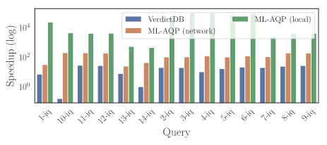
Figure 8. Speedups in large deployments

ML-AQP (local)	ML-AQP (network)	VerdictDB
$443$-$10^{5}$	$24$-$195$	$0.16$-$28$

Table 2. Minimum-Maximum speedups at the Cloud

To be more concise, the min/max speedup benefits of the compared systems are shown at Table 2. As evident, the local deployment is orders of magnitude faster than both VerdictDB and an over the network deployment. We also report on average response times and the response times at the $95^{\text{th}}$ percentile for all systems.

System	Time (sec)	$95^{\text{th}}$ percentile (sec)
Redshift	$55\pm 75$	$142$
VerdictDB	$49\pm 120$	$300$
ML-AQP (network)	$0.78\pm 1.82$	$2.68$
ML-AQP (local)	$0.02\pm 0.08$	$0.25$

Table 3. Performance at the Cloud

The results are shown in Table 3. The first thing we notice, is that although VerdictDB has less mean response time than Redshift, at the $95^{\text{th}}$ percentile it is slower, possibly due to overheads of VerdictDB in deciding which samples to process. In addition, both the network and local deployments for ML-AQP offer mean sub-second latencies and only $2.68$ seconds at the $95^{\text{th}}$ for network.

6.4. Training Overhead

As stated earlier, ML-AQP has to go through Training mode initially. At this stage, previously executed queries are used to train a variety of models and learn to predict the answers of future aggregate queries. Ideally training the models would happen locally at Data Scientist’s machines so as not to incur additional costs of repeatedly training and fine tuning the models in the Cloud. Therefore, in this experiment we measure the Training Time required to build a model with varying number of queries. We run this experiment locally on a single machine with an Intel(R) Core(TM) i7-6700 CPU @3.40GHz, 16GB RAM and 1TB HDD to demonstrate this capability. We compare this to the sample building time of VerdictDB with an increasing sample ratio. We use the TPC-H data set at $1$GB. At each iteration $3$ samples are built on the main fact tables.

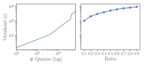
Figure 9. (Left) Training overhead for an increasing number of queries (x-axis) (Right) Sample preparation time for VerdictDB

Figure 9 shows the result of this experiment. The sample preparation time for VerdictDB, Figure 9(right), increases linearly and even for $0.1$ ratio at $1$GB, takes longer than training ML-AQP on $4$ million queries. At $6+$ million queries, this overhead is still less than the sample preparation time for VerdictDB at $0.6$ ratio. To put this in context, for ML-AQP to train on queries generated for Instacart, on $4,000$ for AVG queries took $1.1$ seconds and for SUM $3.3$ seconds. For TPC-H it took, less than a second to train each model. The only exception was for COUNT as its associated queries included a large number of groups $(>50,000)$ and took $326$ seconds to train on around $5$ million training examples in total. It is also important to note that sampling based AQP engines are susceptible to the size of the data set. In this experiment, we are only using $1$GB of data, as the size increases, sample preparation time is expected to increase, too. This would not be a problem for ML-AQP as it is only affected by the number of queries and it is not, at any point, affected by the size of the underlying data set. In conclusion, both approaches, sampling-based AQPs and Query-Driven ML-based AQPs will have ”training” overheads. Their overheads are largely determined by different dimensions and as these solutions are designed to expedite query processing in petabyte scale storage engines we expect ML-AQPs overhead to be much less.

6.5. Accuracy

6.5.1. Accuracy on TPC-H & Instacart

To assess the accuracy of ML-AQP we measure the Relative Error(park2018verdictdbaqp, ; park2017databaseaqp, ; agarwal2013blinkdbaqp, ; kandula2016quickraqp, ) across all the query templates of both Instacart and TPC-H. ML-AQP was trained on past queries generated as described in Section 6.1. Three models were trained using LightGBM to answer Instacart queries, one for each AF involved. For TPC-H, 11 models were trained using XGBoost as the queries were largely referring to AFs on different attributes. The number of rounds were set to $10^{4}$ with early stopping when no more improvement was shown. Objective was set to squared_error. We compare our results with VerdictDB, which created samples over the large fact tables at ratios of $1\%$/$10\%$.

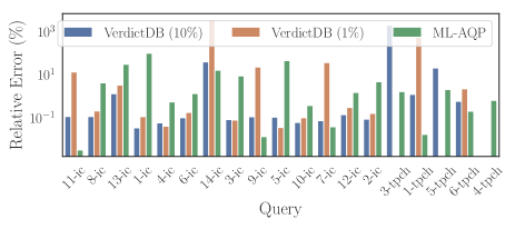
Figure 10. Relative Errors for each query in TPC-H & Instacart

An initial set of results is shown at Figure 10. A first impression is that both systems perform really well over a large range of queries. Please note that the results show the average relative error over each query template. Where for each query template multiple, $>50$, queries were executed with random predicate values as described in (6.1). ML-AQP is able to accurately answer $80\%$ of queries for Instacart and $100\%$ of the selected TPC-H queries with relative error below $10\%$. We can also visually discern that ML-AQP outperforms VerdictDB for many queries. VerdictDB at $1\%$ was not able to answer accurately queries that have a large number of groups, such as $14$-ic and in some cases the groups returned by VerdictDB did not match the ones returned by the engine ($3$-tpch, $5$-tpch). For ML-AQP, queries 1-ic and 5-ic produce large relative errors. This is understandable as these queries include no predicates and are simply the results over a full scan of the table (ie are simple SELECT AF FROM T). The results of such queries can easily be cached. ML-AQP is not expected to answer such queries as the meta-vector $\mathbf{m}$ is filled with nan values, to which the model simply ignores as there are no patterns to be learned.

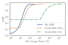
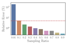
Figure 11. (Left) CDFs of relative error per group in a GROUP-BY query (right) Relative error for an increasing sampling ratio with the mean relative error for ML-AQP as a horizontal line.

We also measure the relative error on a per-group basis. Especially, for query $14$-ic where a large number of groups are present we notice high relative error. Figure 11(left), shows the CDF of the relative error across groups for all three systems. ML-AQP outperforms VerdictDB at both sampling ratios ($1\%$, $10\%$), which shows that it can accurately estimate the aggregates across groups. Given the prior discussion we do not mean to say that sampling based engines have less accuracy. Instead, at a small sampling ratio the benefits are not great and the large trade-off between accuracy and speed makes their use inappropriate. Hence, sampling based engines can be used in parallel to ML-AQP, when the analyst needs more accurate answers and they are willing to sacrifice some of the efficiency for it, as also suggested by Figure 3. So, the systems can co-exist if we use sampling based engines with a higher sampling ratio as the expected error over all queries decreases as is shown at Figure 11(right).

6.5.2. Accuracy on range queries over spatio-temporal data.

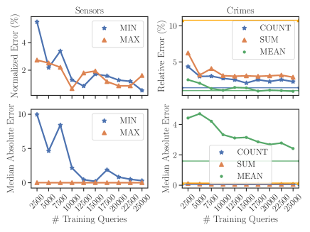
Figure 12. Accuracy over Sensors and Crimes for an increasing number of training queries and over different AFs. (Top) Relative/Normalized Error (Bottom) Median Absolute Error. (Right Column) For Crimes the accuracy of VerdictDB is plotted as horizontal lines.

We have also measured the accuracy of ML-AQP in predicting the responses of range-queries over spatio-temporal data sets. Specifically, multiple synthetic queries are executed over Crimes restricting its spatial dimensions and returning a response COUNT, MEAN or SUM over other attributes included in the data set. Namely COUNT returns the number of recorded incidents within the defined area, MEAN is the average Beat number which is a police defined number describing the area, and SUM of the arrests over the specified area. For Sensors we restricted the temporal dimensions and extract the MIN(temperature) and MAX(humidity). All of the results at Figure 12(top) show that the relative error is below the targeted $10\%$ for this kind of data sets and conntinues dropping as more queries are being used for training the models. We also plot the accuracy for VerdictDB ($1\%$) as horizontal lines only for the Crimes data set as VerdictDB does not support MIN/MAX aggregates. Note that for Sensors, we report on the Normalized Error $|\frac{y-\hat{y}}{\overline{y}}|$, which computes the absolute difference divided by the mean response. The reason is that for this workload, the values are really small ($\mu=9$) and the measured relative error is not robust as it might report a $50\%$ error even if $y=2$ and $\hat{y}=1$. This is also encountered in (kandula2019experiencesaqp, ) and similar technique is employed. To provide more context as to how close the predictions are in relation to the true response, we also provide results on the Median Absolute Error (MAE) at Figure 12(bottom). It is a well known metric in the ML community that is robust to outliers indicating the median of the absolute error between $y$ and $\hat{y}$. As evidenced, the absolute difference is small for all aggregates and data sets and continues to drop as more queries are used for training. The accuracy obtained is similar to VerdictDB’s with ML-AQP having lower relative error for COUNT. In addition, we stress the fact that we are able to predict the responses for MIN and MAX that to our knowledge are not supported by most AQP systems. In addition, as the number of queries increase, we see a drop in relative error suggesting that more accurate predictions can be obtained. Overall, the results of this experiment show that ML-AQP is able to support a wide variety of aggregates over a diverse set of data sets.

6.5.3. Accuracy on error estimation

We study the effectiveness of the prediction intervals constructed using QR. For this experiment we train two LightGBM models on quantile loss, with parameters n_estimators$=1500$ and l_rate$=0.001$. We set $t=0.95$ and train the two models using alpha$=1-t$ and alpha$=t$. This effectively creates a prediction interval that would ideally provide a coverage rate of $90\%$. Coverage rate is used in other work to assess prediction intervals (lei2018distributionconformal, ; foygel2019predictive, ) and is essentially an empirical estimate of the predictions that will fall within the proposed interval. It is computed using a held-out set of queries. Specifically, the two models generate responses for $\hat{y}_{5^{\text{th}}}$ and $\hat{y}_{95^{\text{th}}}$. We test each true value $y$ on $\hat{y}_{5^{\text{th}}}\leq y\leq\hat{y}_{95^{\text{th}}}$ and report the ratio of queries where the condition is true. We used the queries of Instacart and conduct this experiment on three different AFs COUNT, SUM, AVG.

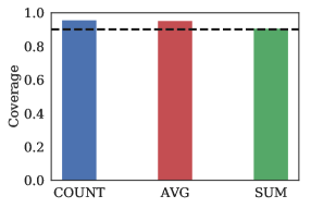
Figure 13. Coverage Ratio for different AFs. Horizontal line drawn at $90\%$

The results at Figure 13 confirm, that empirically a value lies within the interval, provided by QR estimates, by an estimated probability $>0.9$. In short, using QR, ML-AQP is able to provide good probabilistic intervals for the true answer. Using this interval the user can choose whether they trust the prediction or they wish to get a more accurate estimate using an S-AQP or the data warehouse engine.

6.6. Storage

For this experiment, we measure the Storage overhead of ML-AQP. At the end of the Training phase we deploy ML models at analysts devices or a central device. Measuring the storage overhead and ensuring that this is adequately small is of great importance. We expect orders of magnitude smaller storage footprint than sampling based AQP engines as we neither store any of the data nor any of the queries used for training. We initially examine how much memory is required by a model with increased complexity. The main factor contributing to the size of the selected ML models (GBMs) is the number of trees and their depth.

Figure 14. Increasing number of trees (x-axis) and size in kilobytes

Figure 14 shows an increase in the total storage required by an increasing number of trees. For conducting the experiments over Instacart and TPC-H the number of trees never exceeded $1700$ with some AFs requiring as little as $100$ trees. ML-AQP requires additional storage for encoding categorical values and for caching values obtained from queries with GROUP-BY clauses. For instance for Instacart, there are $50,000$ categorical values and ML-AQP requires an extra $4$MB (on top of the storage required by the models). This cost increases linearly as the number of labels increase. Accounting for all of this and even any required modules by the implementation of ML-AQP still does not match the storage overhead required by sampling based AQP. To put this in context, Instacart requires $2.4$GB of storage for its tables. To sample its main fact tables orders and order_products at $0.1$, VerdictDB required $1.8$GB in total. On the other hand, ML-AQP requires a mere $15.5$MB to cover the aggregate queries issued against Instacart, this includes all models and catalogues. Given this information, we can safely assert that ML-AQP is extremely light-weight and can easily reside in main memory during analysis.

6.7. Updates Adaptation

We conduct an experiment to assess ML-AQP’s detection mechanisms for updates in data and workload. As we have elaborated we need to identify cases where $p(y)$ and $p(\mathbf{m})$ change by observing queries executed at the data warehouse without accessing any data. Monitoring actual insertions/updates/deletions could prove futile as the distribution of $y$ might not be changing. For this experiment we use two distributions $p_{1}(\mathbf{m},y)$ and $p_{2}(\mathbf{m},y)$. The distributions for parameters $\mathbf{m}$ are multivariate Normal distributions initialized randomly at the data space of Crimes data set and the answers $y$ are the actual answers for COUNT over the same data set. We first test for data shift detection. In this experiment we obtain the empirical distribution function of $p_{1}(y)$ and conduct the KS test at regular intervals. At a specific point in time we change to $p_{2}(y)$ which we then expect that KS statistic will go over the threshold. The results at Figure 15(left) show that as the distribution shifts the KS statistic increases and becomes larger than $c(a)\sqrt{\frac{n+m}{nm}}$ as soon as the data shift happens (vertical dotted line). In addition, Figure 15(right) shows when the KS statistic fires relative to the impact of updates on $p(y)$ indicating that the model would be updated before relative error increases dramatically.

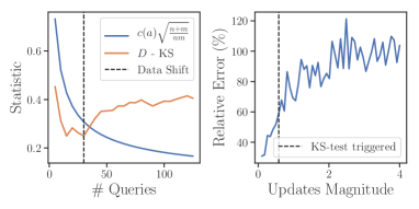
Figure 15. (Left) x-axis; Number of queries processed initially from $p_{1}$ and then from $p_{2}$; y-axis; measured statistic (Right) Updates Magnitude and firing of the KS statistic before relative error increases.

We perform a similar experiment to assess the detection of a workload shift. Again,we have two different distributions, where initially queries are observed from the first distribution and at a specific point in time queries are sampled from the other distribution. We monitor Cheybyshev’s inequality and detect whether the inequality has been violated to trigger a workload shift. The results shown at Figure 16 denote that as the workload changes (indicated by the vertical dotted line) the threshold (horizontal dotted line) provided by the inequality is exceeded and we can successfully detect whether the patterns have shifted and adapt accordingly. In general, in the face of data or workload updates ML-AQP is able to appropriately detect and adapt to such changes.

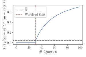
Figure 16. Number of monitored queries and probability of exceeding $k$ standard deviations along with Chebyshev’s inequality threshold.

7. Related Work

To meet the needs of interactive query processing in large analytic environments various big data engines (armbrust2015spark, ; dean2008mapreduce, ; zaharia2016apache, ) and columnar databases (gupta2015amazon, ) have been developed. However, the goal of truly interactive analysis still remains elusive, as such engines produce exact results. Their results have to be computed over large quantities of data. Therefore, research in AQP has been pretty strong the last decades (zeng2015gaqp, ; potti2015daqaqp, ; olma2019tasteraqp, ; acharya1999aquaaqp, ; park2017databaseaqp, ; park2018verdictdbaqp, ; agarwal2013blinkdbaqp, ; kandula2016quickraqp, ; kandula2019experiencesaqp, ; hellerstein1997onlineaqp, ; chaudhuri2017approximateaqp, ; babcock2003dynamicaqp, ; ma2019dbest, ; garofalakis2001approximate, ) and still the list is not exhaustive. We can categorize most AQP engines to sampling based AQP engines (agarwal2013blinkdbaqp, ; park2018verdictdbaqp, ; olma2019tasteraqp, ) and online aggregation engines (zeng2015gaqp, ; hellerstein1997onlineaqp, ). Sampling based AQP engines create samples over some (or all) of the columns in tables and produce answers with error guarantees based on samples. On the other hand, online aggregation engines produce a result as quickly as possible and then keep on refining it as more and more data are processed until the user stops the query execution. However, AQP is struggling to find its way through the industry. A notable approach is QuickR developed from Microsoft (kandula2016quickraqp, ; kandula2019experiencesaqp, ) but there is more work to be done.

More recently we see the deployment of ML models to a wide variety of data management problems: selectivity estimation (dutt2019selectivity, ; cardinalitydeeplearning, ; anagnostopoulos2017query, ; anagnostopoulos2015learning, ; ortiz2019empirical, ; kipf2018learned, ; sun2019end, ; yang2019selectivity, ; woltmann2019cardinality, ), query optimization (neo, ), in which ML is used to decide on a query plan, or to create indexes (kraska2018case, ), for expediting visualisation (wang2018neuralcubes, ) and to AQP (ma2019dbest, ; hilprecht2019deepdb, ; thirumuruganathan2019approximate, ; kulessa2018model, ). We believe that this approach can be fruitful if used with care. This is why we are not aiming to replace already existing AQP engines or data analytic systems and instead provide an addition to the stack. We believe the user needs to have a choice considering the trade-offs between speed and accuracy. As such our approach is similar to the recent trend of applying ML over data management problems, in that we employ ML models for AQP. Approaches such as (ortiz2019empirical, ; cardinalitydeeplearning, ; kipf2018learned, ; sun2019end, ; yang2019selectivity, ; woltmann2019cardinality, ) make use of ML to estimate cardinalities for their use in a query optimization setting. Similar methodologies are adopted in that first features are extracted either from data or from queries and subsequently used for training models. This is to be expected as any relevant work that makes use of ML needs to follow this process. However, all of the aforementioned works focus on cardinality estimation and not on AQP. In addition they follow different modelling/vectorization for the queries, use different ML models and none of the works explicitly address data/workload updates and error guarantees. Perhaps the most similar work to ours is NeuralCubes (NC) (wang2018neuralcubes, ) in which the authors describe a query-driven ML-based system to be used as a visualisation backend engine using AQP (COUNT/AVERAGE) answers. Compared to NC, ML-AQP (i) provides error guarantees, (ii) support updates in both data and workload, (iii) support more AFs, (iv) explicitly provide information on training/storage/prediction-serving overheads, and (v) provide all that with inherently simple, easy to understand ML models. We have conducted experiments based on two data sets that were used in NC and report on Relative Absolute Error (RAE) which is the metric used in NC. ML-AQP’s RAE for BK-Austin was $3.9\%$ (where NC is at $3.88\%$) and for BK-NYC, RAE was $3.6\%$ (where NC is at $4.25\%$). The results suggest better or similar accuracy over NC with a much smaller training overhead–ML-AQP trains its models $>10X$ faster than NC on weaker hardware.

Compared to other approaches focusing on ML for AQP such as (ma2019dbest, ; hilprecht2019deepdb, ; thirumuruganathan2019approximate, ; kulessa2018model, ) ML-AQP neither learns from data nor uses data to construct samples or models. ML-AQP employs a novel query-driven method, based on vectorized representations of previously executed queries and their results and is oblivious to the underlying data distribution. In addition, ML-AQP’s focus is not solely in COUNT/SUM/AVG as most works (hilprecht2019deepdb, ; thirumuruganathan2019approximate, ; kulessa2018model, ) but offers support for any kind of AF through its AF agnostic methodology. Nevertheless, data-driven approaches are surely a promising avenue and we believe all of these approaches could complement each other. In cases where;i) data sets are massive, ii) no models or samples can be built and stored efficiently, and iii) there is a low cost requirement, ML-AQP appears to be more favorable.

8. Conclusions

In this paper we described ML-AQP, whose salient feature is that it develops ML models over (small numbers of) previously executed queries and their answers, instead of developing models or samples over massive base tables. The models are extremely compact and simple, avoiding using complex deep learning networks. Despite this, ML-AQP can provide answers efficiently, offering up to $5$ orders of magnitude speedups in large deployments with small relative errors. Specifically, queries and their answers are transformed into a custom vectorized representation. This representation, allows training ML models that learn patterns to predict future query answers. Also, ML-AQP can bound errors of its answers by employing prediction intervals constructed using Quantile Regression models. In addition, updates to data and changes in query workloads can be handled effectively. Moreover, it can support any aggregate queries, including MIN,MAX (which most AQP systems struggle to address), along with GROUP-BYs. Experiments substantiate that ML-AQP can ensure low errors while introducing dramatic efficiency gains with small memory/storage footprints, and supporting all aggregate functions. ML-AQP, thus, shows a promising method into how ML models can be incorporated for AQP, avoiding the pitfalls of dealing with massive data sets.

Appendix A Appendix

A.1. Restricting Dimensionality of the Query Representation

As the number of columns (attributes, dimensions) gets larger, our representation will be moving towards a high-dimensional space causing problems to our underlying ML models. One way to tackle this is to use unsupervised dimensionality reduction techniques [51], which will reduce the dimensionality of our given query vectors. Another, more straightforward way to tackle this is to restrict the number of columns we built our ML models over. As examined queries focus on a subset of the original column set [9, 60], allowing us to use a heuristic to build ML models only over the most frequently used columns or the columns of the highest importance to the analysts. Especially, in the case of spatio-temporal data sets the focus is usually on the spatial and temporal dimensions to which an analyst applies filters and then examines descriptive statistics over other columns.

A.2. Sensitivity Analysis

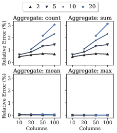
Figure 17. Relative Error (y-axis) measured across different aggregates with an increasing number of columns/attributes (x-axis) and a varying number of predicates set randomly.

In this section of our experimental analysis, we study a variety of variables contributing to the accuracy of our solution. For these experiments, we use the synthetic dataset to control the number of attributes and predicates set. Queries with meta-vectors up to $200$, $\mathbf{m}\in\mathbb{R}^{200}$, are executed over uniform spaces with the number of set predicates up to $50$ . All predicates are numerical and each query vector is associated with a response. The predicates essentially define range queries over the respective columns. To put this in perspective, real workloads expect a median number of columns selected in a query around $8$ [31] with a more recent estimate reporting that $90\%$ of queries use around $1-6$ [30] columns with a maximum reaching $12$. We increase the number of predicates and columns to study the effects on accuracy. We initially train the models on a constant number of queries $10,000$ and vary the number of predicates and columns/attributes. In addition, we test different aggregates, COUNT, SUM, MEAN/AVG and MAX, to examine their predictability. In essence, ML-AQP is agnostic to what kind of aggregate is being predicted, to ML-AQP an AF applied over an attribute is a response variable to which it tries to identify patterns that can help it minimize the loss $L(y,\hat{y})$.

As can be seen at Figure 17, the relative error increases w.r.t. the number of columns and predicates. Although there is not a notable increase ($2\%$), we can attribute this to the fact that more queries might be needed to learn a more complex space. As the dimensionality of the space (number of columns) increases, the number of predicates increasingly restricts the sub-spaces defined by the queries. In addition, For MEAN and MAX, we do not observe large differences in relative error. Closely, examining the workloads we notice that the Coefficient of Variation (CoV), defined by the standard deviation to the mean ration: $\frac{\sigma}{\mu}$ is $0.08$ for the response $y$ of MEAN and $0.01$ for the response MAX. Where the CoV shows the extent of the variability in relation to the mean. A CoV value closer to $1$ indicates high variability. Therefore, ML-AQP might be able to learn their distributions with less queries.

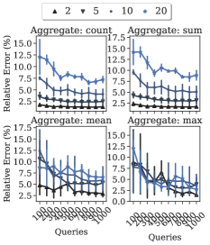
Figure 18. Relative Error (y-axis) measured across different aggregates with an increasing number of queries (x-axis) used for training.

Figure 18 shows how relative error decreases as the number of queries that a model is trained on increases. For all aggregates, we notice that the effect the number of queries has started to diminish and nothing more can be learned. This provides an approximation to the number of queries needed to model the specific aggregates under this workload. It also denotes that after exceeding a certain number of queries, we should then focus on the complexity of our model to further decrease the relative error. In addition, for MEAN and MAX, we see high standard deviation for relative error across settings, especially when the number of queries is small. This advises us that as the number of queries is small, relative error is largely determined by the complexity of the workload (dimensionality, sparsity). However, as more and more queries are being used to train the models this effect fades away.

References

- [1] Crimes workload. URL :https://archive.ics.uci.edu/ml/datasets/Query+Analytics +Workloads+Dataset. Accessed: 2019-06-28.
- [2] Instacart. URL :https://www.instacart.com/datasets/grocery-shopping-2017. Accessed: 2019-06-28.
- [3] Instacart queries. https://github.com/verdictdb/verdict/wiki/Instacart-Queries.
- [4] Tpc-h. http://www.tpc.org/tpch/.
- [5] Crimes - 2001 to present. URL: https://data.cityofchicago.org/Public-Safety/Crimes-2001-to-present/ijzp-q8t2, 2018. Accessed: 2018-08-10.
- [6] Intel lab data. URL: http://db.csail.mit.edu/labdata/labdata.html, 2019. Accessed: 2019-04-10.
- [7] S. Acharya, P. B. Gibbons, V. Poosala, and S. Ramaswamy. The aqua approximate query answering system. In ACM Sigmod Record, volume 28, pages 574–576. ACM, 1999.
- [8] S. Agarwal, H. Milner, A. Kleiner, A. Talwalkar, M. Jordan, S. Madden, B. Mozafari, and I. Stoica. Knowing when you’re wrong: building fast and reliable approximate query processing systems. In Proceedings of the 2014 ACM SIGMOD international conference on Management of data, pages 481–492. ACM, 2014.
- [9] S. Agarwal, B. Mozafari, A. Panda, H. Milner, S. Madden, and I. Stoica. Blinkdb: queries with bounded errors and bounded response times on very large data. In Proceedings of the 8th ACM European Conference on Computer Systems, pages 29–42. ACM, 2013.
- [10] C. C. Aggarwal, A. Hinneburg, and D. A. Keim. On the surprising behavior of distance metrics in high dimensional space. In International conference on database theory, pages 420–434. Springer, 2001.
- [11] C. Anagnostopoulos and P. Triantafillou. Learning set cardinality in distance nearest neighbours. In 2015 IEEE international conference on data mining, pages 691–696. IEEE, 2015.
- [12] C. Anagnostopoulos and P. Triantafillou. Query-driven learning for predictive analytics of data subspace cardinality. ACM Transactions on Knowledge Discovery from Data (TKDD), 11(4):47, 2017.
- [13] M. Armbrust, R. S. Xin, C. Lian, Y. Huai, D. Liu, J. K. Bradley, X. Meng, T. Kaftan, M. J. Franklin, A. Ghodsi, et al. Spark sql: Relational data processing in spark. In Proceedings of the 2015 ACM SIGMOD international conference on management of data, pages 1383–1394. ACM, 2015.
- [14] B. Babcock, S. Chaudhuri, and G. Das. Dynamic sample selection for approximate query processing. In Proceedings of the 2003 ACM SIGMOD international conference on Management of data, pages 539–550. ACM, 2003.
- [15] L. Bottou. Stochastic gradient descent tricks. In Neural networks: Tricks of the trade, pages 421–436. Springer, 2012.
- [16] S. Chaudhuri, B. Ding, and S. Kandula. Approximate query processing: No silver bullet. In Proceedings of the 2017 ACM International Conference on Management of Data, pages 511–519. ACM, 2017.
- [17] T. Chen and C. Guestrin. Xgboost: A scalable tree boosting system. In Proceedings of the 22nd acm sigkdd international conference on knowledge discovery and data mining, pages 785–794. ACM, 2016.
- [18] J. Dean and S. Ghemawat. Mapreduce: simplified data processing on large clusters. Communications of the ACM, 51(1):107–113, 2008.
- [19] A. Dutt, C. Wang, A. Nazi, S. Kandula, V. Narasayya, and S. Chaudhuri. Selectivity estimation for range predicates using lightweight models. Proceedings of the VLDB Endowment, 12(9):1044–1057, 2019.
- [20] B. Efron and R. J. Tibshirani. An introduction to the bootstrap. CRC press, 1994.
- [21] R. Foygel Barber, E. J. Candes, A. Ramdas, and R. J. Tibshirani. Predictive inference with the jackknife+. arXiv preprint arXiv:1905.02928, 2019.
- [22] J. Friedman, T. Hastie, and R. Tibshirani. The elements of statistical learning, volume 1. Springer series in statistics New York, NY, USA:, 2001.
- [23] J. H. Friedman. Greedy function approximation: a gradient boosting machine. Annals of statistics, pages 1189–1232, 2001.
- [24] M. N. Garofalakis and P. B. Gibbons. Approximate query processing: Taming the terabytes. In VLDB, pages 343–352, 2001.
- [25] A. Gupta, D. Agarwal, D. Tan, J. Kulesza, R. Pathak, S. Stefani, and V. Srinivasan. Amazon redshift and the case for simpler data warehouses. In Proceedings of the 2015 ACM SIGMOD international conference on management of data, pages 1917–1923. ACM, 2015.
- [26] A. Hall, A. Tudorica, F. Buruiana, R. Hofmann, S.-I. Ganceanu, and T. Hofmann. Trading off accuracy for speed in powerdrill. 2016.
- [27] J. M. Hellerstein, P. J. Haas, and H. J. Wang. Online aggregation. In Acm Sigmod Record, volume 26, pages 171–182. ACM, 1997.
- [28] B. Hilprecht, A. Schmidt, M. Kulessa, A. Molina, K. Kersting, and C. Binnig. Deepdb: Learn from data, not from queries! arXiv preprint arXiv:1909.00607, 2019.
- [29] S. Idreos, O. Papaemmanouil, and S. Chaudhuri. Overview of data exploration techniques. In Proceedings of the 2015 ACM SIGMOD International Conference on Management of Data, pages 277–281. ACM, 2015.
- [30] S. Kandula, K. Lee, S. Chaudhuri, and M. Friedman. Experiences with approximating queries in microsoft’s production big-data clusters. Proceedings of the VLDB Endowment, 12(12):2131–2142, 2019.
- [31] S. Kandula, A. Shanbhag, A. Vitorovic, M. Olma, R. Grandl, S. Chaudhuri, and B. Ding. Quickr: Lazily approximating complex adhoc queries in bigdata clusters. In Proceedings of the 2016 International Conference on Management of Data, pages 631–646. ACM, 2016.
- [32] G. Ke, Q. Meng, T. Finley, T. Wang, W. Chen, W. Ma, Q. Ye, and T.-Y. Liu. Lightgbm: A highly efficient gradient boosting decision tree. In Advances in Neural Information Processing Systems, pages 3146–3154, 2017.
- [33] A. Kipf, T. Kipf, B. Radke, V. Leis, P. Boncz, and A. Kemper. Learned cardinalities: Estimating correlated joins with deep learning. arXiv preprint arXiv:1809.00677, 2018.
- [34] A. Kipf, D. Vorona, J. Müller, T. Kipf, B. Radke, V. Leis, P. Boncz, T. Neumann, and A. Kemper. Estimating cardinalities with deep sketches. In Proceedings of the 2019 International Conference on Management of Data, SIGMOD ’19, pages 1937–1940, New York, NY, USA, 2019. ACM.
- [35] R. Koenker and K. F. Hallock. Quantile regression. Journal of economic perspectives, 15(4):143–156, 2001.
- [36] T. Kraska, A. Beutel, E. H. Chi, J. Dean, and N. Polyzotis. The case for learned index structures. In Proceedings of the 2018 International Conference on Management of Data, pages 489–504. ACM, 2018.
- [37] M. Kuhn and K. Johnson. Applied predictive modeling, volume 26. Springer, 2013.
- [38] M. Kulessa, A. Molina, C. Binnig, B. Hilprecht, and K. Kersting. Model-based approximate query processing. arXiv preprint arXiv:1811.06224, 2018.
- [39] J. Lei, M. GŚell, A. Rinaldo, R. J. Tibshirani, and L. Wasserman. Distribution-free predictive inference for regression. Journal of the American Statistical Association, 113(523):1094–1111, 2018.
- [40] Z. Liu and J. Heer. The effects of interactive latency on exploratory visual analysis. IEEE Transactions on Visualization & Computer Graphics, pages 1–1, 2014.
- [41] Q. Ma and P. Triantafillou. Dbest: Revisiting approximate query processing engines with machine learning models. In Proceedings of the 2019 International Conference on Management of Data, pages 1553–1570. ACM, 2019.
- [42] R. Marcus, P. Negi, H. Mao, C. Zhang, M. Alizadeh, T. Kraska, O. Papaemmanouil, and N. Tatbul. Neo: A learned query optimizer. Proc. VLDB Endow., 12(11):1705–1718, July 2019.
- [43] N. Meinshausen. Quantile regression forests. Journal of Machine Learning Research, 7(Jun):983–999, 2006.
- [44] M. Olma, O. Papapetrou, R. Appuswamy, and A. Ailamaki. Taster: Self-tuning, elastic and online approximate query processing. In 2019 IEEE 35th International Conference on Data Engineering (ICDE), pages 482–493. IEEE, 2019.
- [45] J. Ortiz, M. Balazinska, J. Gehrke, and S. S. Keerthi. An empirical analysis of deep learning for cardinality estimation. arXiv preprint arXiv:1905.06425, 2019.
- [46] H. Papadopoulos, V. Vovk, and A. Gammerman. Regression conformal prediction with nearest neighbours. Journal of Artificial Intelligence Research, 40:815–840, 2011.
- [47] Y. Park, B. Mozafari, J. Sorenson, and J. Wang. Verdictdb: universalizing approximate query processing. In Proceedings of the 2018 International Conference on Management of Data, pages 1461–1476. ACM, 2018.
- [48] Y. Park, A. S. Tajik, M. Cafarella, and B. Mozafari. Database learning: Toward a database that becomes smarter every time. In Proceedings of the 2017 ACM International Conference on Management of Data, pages 587–602. ACM, 2017.
- [49] N. Potti and J. M. Patel. Daq: a new paradigm for approximate query processing. Proceedings of the VLDB Endowment, 8(9):898–909, 2015.
- [50] Y. Romano, E. Patterson, and E. J. Candès. Conformalized quantile regression. arXiv preprint arXiv:1905.03222, 2019.
- [51] S. T. Roweis and L. K. Saul. Nonlinear dimensionality reduction by locally linear embedding. science, 290(5500):2323–2326, 2000.
- [52] K. Sato. An inside look at google bigquery. White paper, URL: https://cloud. google. com/files/BigQueryTechnicalWP. pdf, 2012.
- [53] G. Shafer and V. Vovk. A tutorial on conformal prediction. Journal of Machine Learning Research, 9(Mar):371–421, 2008.
- [54] I. Steinwart, A. Christmann, et al. Estimating conditional quantiles with the help of the pinball loss. Bernoulli, 17(1):211–225, 2011.
- [55] J. Sun and G. Li. An end-to-end learning-based cost estimator. Proceedings of the VLDB Endowment, 13(3):307–319, 2019.
- [56] I. Takeuchi, Q. V. Le, T. D. Sears, and A. J. Smola. Nonparametric quantile estimation. Journal of machine learning research, 7(Jul):1231–1264, 2006.
- [57] M. A. Tanner and W. H. Wong. The calculation of posterior distributions by data augmentation. Journal of the American statistical Association, 82(398):528–540, 1987.
- [58] S. Thirumuruganathan, S. Hasan, N. Koudas, and G. Das. Approximate query processing using deep generative models. arXiv preprint arXiv:1903.10000, 2019.
- [59] Z. Wang, D. Cashman, M. Li, J. Li, M. Berger, J. A. Levine, R. Chang, and C. Scheidegger. Neuralcubes: Deep representations for visual data exploration. arXiv preprint arXiv:1808.08983, 2018.
- [60] A. Wasay, X. Wei, N. Dayan, and S. Idreos. Data canopy: Accelerating exploratory statistical analysis. In Proceedings of the 2017 ACM International Conference on Management of Data, pages 557–572. ACM, 2017.
- [61] L. Woltmann, C. Hartmann, M. Thiele, D. Habich, and W. Lehner. Cardinality estimation with local deep learning models. In Proceedings of the Second International Workshop on Exploiting Artificial Intelligence Techniques for Data Management, pages 1–8, 2019.
- [62] Z. Yang, E. Liang, A. Kamsetty, C. Wu, Y. Duan, X. Chen, P. Abbeel, J. M. Hellerstein, S. Krishnan, and I. Stoica. Selectivity estimation with deep likelihood models. arXiv preprint arXiv:1905.04278, 2019.
- [63] M. Zaharia, R. S. Xin, P. Wendell, T. Das, M. Armbrust, A. Dave, X. Meng, J. Rosen, S. Venkataraman, M. J. Franklin, et al. Apache spark: a unified engine for big data processing. Communications of the ACM, 59(11):56–65, 2016.
- [64] K. Zeng, S. Agarwal, A. Dave, M. Armbrust, and I. Stoica. G-ola: Generalized on-line aggregation for interactive analysis on big data. In Proceedings of the 2015 ACM SIGMOD International Conference on Management of Data, pages 913–918. ACM, 2015.
- [65] K. Zeng, S. Gao, B. Mozafari, and C. Zaniolo. The analytical bootstrap: a new method for fast error estimation in approximate query processing. In Proceedings of the 2014 ACM SIGMOD international conference on Management of data, pages 277–288. ACM, 2014.