Universal finite-time thermodynamics of many-body quantum machines
from Kibble-Zurek scaling

Abstract

We demonstrate the existence of universal features in the finite-time thermodynamics of quantum machines by considering a many-body quantum Otto cycle in which the working medium is driven across quantum critical points during the unitary strokes. Specifically, we consider a quantum engine powered by dissipative energizing and relaxing baths. We show that under very generic conditions, the output work is governed by the Kibble-Zurek mechanism, i.e., it exhibits a universal power-law scaling with the driving speed through the critical points. We also optimize the finite-time thermodynamics as a function of the driving speed. The maximum power and the corresponding efficiency take a universal form, and are reached for an optimal speed that is governed by the critical exponents. We exemplify our results by considering a transverse-field Ising spin chain as the working medium. For this model, we also show how the efficiency and power vary as the engine becomes critical.

I Introduction

Advances in quantum science and technology have made possible the laboratory implementation of minimal quantum devices such as heat engines and refrigerators using a variety of platforms that include trapped ions Roßnagel et al. (2016); Maslennikov et al. (2019); von Lindenfels et al. (2019), nitrogen vacancy centers Klatzow et al. (2019), and nuclear magnetic resonance experiments Peterson et al. (2019). Quantum engines (QE) transform heat and possibly other resources into some kind of useful work Gemmer et al. (2009). Their study paves the way to identify quantum effects in their performance. In particular, one may wonder whether there exist scenarios exhibiting a quantum advantage with no classical counterpart Jaramillo et al. (2016); Klatzow et al. (2019); Mukherjee et al. (2020).

To a large extent, the study of quantum engines has been restricted to single-particle systems Kosloff and Rezek (2017). Such devices already display nontrivial features when their operation involves quantum synchronization Jaseem et al. (2020), non-thermal coherent and squeezed reservoirs Scully et al. (2003); Roßnagel et al. (2014); Gardas and Deffner (2015); Niedenzu et al. (2018), quantum measurements Elouard et al. (2017a, b); Cottet et al. (2017) and quantum metrology Hofer et al. (2017); Bhattacharjee et al. (2020), in the presence of quantum coherence over sustained many cycles Watanabe et al. (2017), or in the small action limit, when different cycles become thermodynamically equivalent Uzdin et al. (2015).

Quantum thermal machines with many-body working mediums (WMs) may allow us to harness many-body effects, such as entanglement and other quantum correlations for operation with enhanced power and efficiency Jaramillo et al. (2016). Shortcuts to adiabaticity have been shown to enhance the performance of many body quantum thermal machines Hartmann et al. (2020). Quantum statistics can boost the performance of Szilard engines Kim et al. (2011); Bengtsson et al. (2018). Similarly, the performance of quantum Otto Cycles in both the adiabatic Zheng and Poletti (2015) and finite-time operation Jaramillo et al. (2016) can exhibit an enhancement due to bosonic quantum statistics, while a detrimental one has been predicted in the fermionic case. Other many-particle effects that can be harnessed for the engineering of QE include super-radiance Hardal and Müstecaplıoğlu (2015) and many-body localization Yunger Halpern et al. (2019), while novel configurations become feasible, e.g., by using spin networks Türkpençe et al. (2017). Many-particle QE are also required for scalability and the possibility of suppressing quantum friction during their finite-time operation Deng et al. (2013); del Campo et al. (2014); Beau et al. (2016); Funo et al. (2017); del Campo et al. (2018) which has been explored in the laboratory with trapped Fermi gases Deng et al. (2018); Diao et al. (2018).

Quantum criticality may offer new avenues to boost the performance of heat engines, as a result of the diverging length and time-scales close to a phase transition Sachdev (1999). The enhancement of microscopic fluctuations to approach Carnot efficiency in finite time was proposed in Polettini et al. (2015). Further, the scaling theory of second-order phase transitions has been used to show that the ratio between the output power and the deviation of the efficiency from the Carnot limit can be optimized at criticality Campisi and Fazio (2016). In adiabatic interaction-driven heat engines, quantum criticality has also shown to optimize the output power Chen et al. (2019).

In this work, we introduce a quantum Otto cycle with a working medium that exhibits a quantum phase transition. In particular, we consider the family of free-fermionic models that include paradigmatic instances of critical spin systems such as the quantum Ising and XY chains, as well as higher dimensional models. As a result, our setting is of direct relevance to current efforts for building many-particle QEs, with e.g., trapped ions. We explore how signatures of universality in the critical dynamics of the working medium carry over the finite-time thermodynamics of the heat engine.

Remarkably, we show that the scaling of the work output of such QEs with the driving time follows a universal power law resulting from the Kibble-Zurek mechanism. This result paves the way for the hitherto unexplored field of universal finite-time thermodynamics describing quantum machines driven through quantum critical points. To the best of our knowledge, such a connection has not been explored before, and is the focus of our paper.

In Sec. II, we introduce the model of a many body Otto cycle using a free-Fermionic WM. We discuss Kibble-Zurek scaling and its connection to the output work and power of quantum Otto cycles in Section III.1, while Section III.2 introduces an efficiency bound depending on dynamical critical exponent. We focus on the particular example of a transverse Ising spin chain WM in Sec. IV which is further divided into two subsections depending upon the different phases the WM explores during unitary strokes. We also provide analytical expressions for the energies exchanged in each stroke and compare them with numerics. Finally we conclude in Sec. V.

II Many body Otto Cycle

The use of spins as WM opens a wide range of opportunities recognized early on Geva and Kosloff (1992); Quan et al. (2007). Recent experiments have implemented single-spin quantum heat engine Peterson et al. (2019); von Lindenfels et al. (2019) and test fluctuation theorems in single strokes Batalhão et al. (2014); Smith et al. (2018). WM composed of interacting spins such as multiferroics have been proposed Azimi et al. (2014); Chotorlishvili et al. (2016) whereas it is shown that WMs with cooperative effects boost engine properties Niedenzu and Kurizki (2018). Quantum critical spin systems in quantum thermodynamics have also been considered under adiabatic performance Çakmak et al. (2016); Ma et al. (2017), shortcuts to adiabaticity Çakmak and Müstecaplıoğlu (2019) and the limit of sudden driving Dorner et al. (2012); Nigro et al. (2019). Such settings preclude the study of signatures of universality associated with the quantum critical dynamics in the finite-time protocols, which is our focus.

We consider an Otto cycle with a many-body WM, described by the Hamiltonian

$$H = \sum_{k}\Psi_{k}^{\dagger}\tilde{H}_{k}\Psi_{k},$$

$$\tilde{H}_{k} = (\lambda+a_{k})\sigma^{z}+b_{k}\sigma^{+}+b_{k}^{*}\sigma^{-},$$ (1)

with $\sigma^{+}=(\sigma^{x}+i\sigma^{y})/2$, $\sigma^{-}=(\sigma^{x}-i\sigma^{y})/2$, and $\sigma^{x}$, $\sigma^{y}$, $\sigma^{z}$ being the usual Pauli matrices. Here $\tilde{H}_{k}$ is a $2\times 2$ matrix in a basis given by $\Psi_{k}^{\dagger}=(c_{1k}^{\dagger},c_{2k}^{\dagger})$ where $c_{jk},~{}c_{jk}^{\dagger}$ ($j=1,2$) are fermionic operators for the $k$-th momentum mode. Such a Hamiltonian includes widely studied models, such as the transverse-field Ising and XY chains Bunder and McKenzie (1999); Lieb et al. (1961); Pfeuty (1970); Dziarmaga (2010); Dutta et al. (2015), and the two dimensional Kitaev model Kitaev (2006); Chen and Nussinov (2008); Sengupta et al. (2008), through suitable choices of $\lambda,~{}a_{k}$ and $b_{k}$. This Hamiltonian exhibits a quantum critical point (QCP) at $\lambda=\lambda_{\rm c}$, when the energy gap $\Delta=2\sqrt{(\lambda_{\rm c}+a_{k})^{2}+|b_{k}|^{2}}$ between the ground state and first excited state vanishes, for the critical mode $k=k_{\rm c}$. The density matrix of such a system can be written in a basis consisting of $|0,0\rangle$, $|1_{1k},0\rangle$, $|0,1_{2k}\rangle$, $|1_{1k},1_{2k}\rangle$ where the first index corresponds to presence (1) or absence (0) of $c_{1k}$ fermion. Similarly, the second index corresponds to $c_{2k}$ fermions. It is to be noted that the unitary dynamics generated by the Hamiltonian $\tilde{H}_{k}$ mixes $|1_{1k},0\rangle$, and $|0,1_{2k}\rangle$ only. As we shall see later, the non-unitary dynamics allows mixing along the other two basis too Keck et al. (2017); Bandyopadhyay et al. (2018). We denote the full $4\times 4$ Hamiltonian matrix by $H_{k}$.

Before dwelling on the dynamics in Fourier space, let us briefly discuss its real space counterpart. One of the prominent instances within the family of Hamiltonians in Eq. (1) is that of the Ising and the XY models in a transverse field (we assume a ring geometry) which takes the real-space form

$$H = -\sum_{i}M_{i}\left(c_{i}^{\dagger}c_{i+1}-c_{i}c^{\dagger}_{i+1}\right)$$ (2)

$$+ N_{i}\left(c_{i}^{\dagger}c_{i+1}^{\dagger}-c_{i}c_{i+1}\right)+R_{i}\left(c_{i}^{\dagger}c_{i}-c_{i}c_{i}^{\dagger}\right).$$

Here $i$ denotes the site index, $c_{i},c_{i}^{\dagger}$ are Fermionic annihilation and creation operators, respectively, and $M_{i},~{}N_{i},~{}R_{i}$ are scalars Lieb et al. (1961). Such a Hamiltonian can be generated, for example, using a WM consisting of interacting-Fermions in an optical lattice setup Schreiber et al. (2015). If $M_{i}$, $N_{i}$ and $R_{i}$ are site independent, one can perform Fourier transform of the Hamiltonian to express it in the form of Eq. (1). We shall discuss more on this Hamiltonian in Sec. IV.

The quantum Otto cycle alternates between unitary and nonunitary strokes. We now describe below the four general stages of the Otto cycle in details (see Fig. 1):

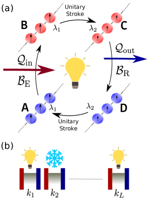
Figure 1: Schematic diagram of a many-body quantum Otto cycle (a) Schematic diagram of a quantum Otto cycle with a many-body system as the working medium. We get a net output work in the heat engine regime (shown by the glowing light bulb). (b) In the equivalent momentum space, the interacting many-body QE can be represented by independent quantum thermal machines corresponding to the different decoupled Fermionic $k$ modes, each acting as a heat engine (shown by glowing light bulbs), or as a refrigerator (shown by the snow-flake), or even as a heat distributor (not shown here).

1. Stroke 1 (${\bf A}\to{\bf B}$): The WM is subjected to a constant Hamiltonian (Eq. (1)) with $\lambda=\lambda_{1}$, while being coupled to a dissipative energizing bath $\mathcal{B}_{\rm E}$ for a time $\tau_{\rm E}$ as shown in Fig. 1a, thus resulting in non-unitary dynamics. We assume $\tau_{\rm E}$ to be large enough so that the WM reaches the steady state.

   In general the dissipative dynamics undergone by the density matrix $\rho(t)$ is given by

   $$\frac{d\rho}{dt}=-i[H,\rho]+\mathcal{D}[\rho]$$ (3)

   with $\hbar$ set to unity, and $\mathcal{D}[\rho]$ is the non-unitary part of the dynamics generated due to the interaction of the system with the bath. The exact form of $\mathcal{D}[\rho]$ depends upon the nature of the bath and its interaction with the system. Here we consider baths with unique steady states. This can be achieved, for example, by coupling the WM to a thermal bath at a finite temperature.

   Alternatively, one can consider Markovian baths coupled locally to the Fermionic modes shown in Eq. (2), with $\mathcal{D}[\rho]$ given by

   $$\mathcal{D}\left[\rho\right] = \sum_{i}\tilde{\kappa}_{i}\left(L_{i}\rho L_{i}^{\dagger}-\frac{1}{2}\{\rho,L_{i}^{\dagger}L_{i}\}\right).$$ (4)

   Here $\tilde{\kappa}_{i}$ is related to system-bath coupling strength for the site $i$, $L_{i}$ are local Lindblad operators that describe the interaction of the Fermion at site $i$ with the bath. For $L_{i}=c_{i}$ (see Eq. (2)) and site independent $\tilde{\kappa}_{i}$, it can be shown that the Fourier transform of $\mathcal{D}[\rho]$ does not mix different modes, so that we arrive at mode-dependent non-interacting local baths in the free-Fermionic representation in momentum space. The existence of non-interacting Fermionic modes implies the state $\rho(t)$ of the many-body WM can be written as $\rho(t)=\bigotimes_{k}\rho_{k}(t)$, with the time-evolution of $\rho_{k}(t)$ given by the differential equation Keck et al. (2017); Bandyopadhyay et al. (2018)

   $$\frac{d\rho_{k}}{dt} = -i[H_{k},\rho_{k}]+\mathcal{D}_{k}[\rho_{k}]$$

   $$\mathcal{D}_{k}[\rho_{k}] = \kappa_{1}^{E}\left(c_{1k}\rho_{k}c_{1k}^{\dagger}-\frac{1}{2}\{c_{1k}^{\dagger}c_{1k},\rho_{k}\}\right)$$ (5)

   $$+ \kappa_{2}^{\rm E}\left(c_{1k}^{\dagger}\rho_{k}c_{1k}-\frac{1}{2}\{c_{1k}c_{1k}^{\dagger},\rho_{k}\}\right)$$

   $$+ \kappa_{3}^{E}\left(c_{2k}\rho_{k}c_{2k}^{\dagger}-\frac{1}{2}\{c_{2k}^{\dagger}c_{2k},\rho_{k}\}\right)$$

   $$+ \kappa_{4}^{\rm E}\left(c_{2k}^{\dagger}\rho_{k}c_{2k}-\frac{1}{2}\{c_{2k}c_{2k}^{\dagger},\rho_{k}\}\right)$$

   Here $\kappa_{j}^{\rm E}$ ($j=1,2,3,4$) are positive constants related to the energizing bath, which depend on the coupling strength between the WM and the bath. The energy exchanged in this stroke is denoted as $\mathcal{Q}_{\rm in}$.

2. Stroke 2 (${\bf B}\to{\bf C}$): The system is decoupled from the bath at ${\bf B}$ and $\lambda$ is varied linearly in time as $t/\tau_{1}$ from $\lambda_{1}$ (at ${\bf B}$) to $\lambda_{2}$ (at ${\bf C}$) in a time interval $\tau_{1}$, such that the WM undergoes a unitary dynamics described by

   $$\frac{d\rho_{k}}{dt}=-i[H_{k},\rho_{k}].$$ (6)

   We consider $\lambda_{1}>\lambda_{2}$ in this paper. Work is done on or by the system in this stroke.

3. Stroke 3 (${\bf C}\to{\bf D}$): The WM is now coupled to a relaxing bath $\mathcal{B}_{\rm R}$ at C of Fig. 1a, for a time duration $\tau_{\rm R}$, at a constant $\lambda=\lambda_{2}$. The evolution equation will be similar to that given in Eq. (5) with appropriate couplings $\kappa_{1}^{\rm R}\dots\kappa_{4}^{\rm R}$ related to $\mathcal{B}_{\rm R}$. Quantum critical dynamics are more pronounced for systems close to their ground states. Consequently, universal scaling behavior is to be expected by considering a relaxing bath which takes the WM to its ground state in this stroke. In principle, we can tune the relaxing bath coupling parameters such that it either takes the system to its ground state or to some steady state corresponding to the bath parameters. We denote the energy exchanged in this stroke with $\mathcal{Q}_{\rm out}$.

4. Stroke 4 (${\bf D}\to{\bf A}$): The system is decoupled from $\mathcal{B}_{\rm R}$ and $\lambda_{2}$ (at ${\bf D}$) is varied back to $\lambda_{1}$ (at ${\bf A}$) linearly in a time interval $\tau_{2}$ as $t/\tau_{2}$. Once again, work is done on or by the system in this stroke.

   One can operate the QE in a steady state cycle, by repeating the above described cycle. It is to be noted that depending upon the values of $\lambda_{1}$ and $\lambda_{2}$, we may or may not cross the critical point. We consider both of these possibilities in this paper.

At the end of any stroke, the energy of the system is calculated using

$$\mathcal{E}=\text{Tr}(H\rho)=\sum_{k}\text{Tr}(H_{k}\rho_{k}).$$ (7)

We choose the parameters $\kappa_{1}^{\rm E},\dots,\kappa_{4}^{\rm E},\kappa_{1}^{\rm R},\dots,\kappa_{4}^{\rm R}$, $\lambda_{1}$ and $\lambda_{2}$ such that energy $\mathcal{Q}_{\rm in}$ is absorbed when coupled to $\mathcal{B}_{\rm E}$ in stroke 1, while a smaller amount $\mathcal{Q}_{\rm out}$ is released when coupled to $\mathcal{B}_{\rm R}$ in stroke 3, such that the setup operates as a heat engine, with a net output work $\mathcal{W}=-\left(\mathcal{Q}_{\rm in}+\mathcal{Q}_{\rm out}\right)$. We assume the following sign convention for the energy flows: $\mathcal{Q}_{\rm in}$, $\mathcal{Q}_{\rm out},\mathcal{W}$ are positive (negative) if the WM energy increases (decreases). For the Otto cycle to operate as a heat engine, we need $\mathcal{Q}_{\rm in}>0$, $\mathcal{Q}_{\rm out}<0,\mathcal{W}<0$. On the other hand, $\mathcal{Q}_{\rm in}<0,~{}\mathcal{Q}_{\rm out}>0,~{}\mathcal{W}>0$ corresponds to a refrigerator, and $\mathcal{Q}_{\rm out}<0,~{}\mathcal{W}>0$ denotes a heat distributor Mukherjee et al. (2016). We characterize the performance of the heat engine in terms of its efficiency $\eta$

$$\eta=\frac{\mathcal{Q}_{\rm in}+\mathcal{Q}_{\rm out}}{\mathcal{Q}_{\rm in}}=-\frac{\mathcal{W}}{\mathcal{Q}_{\rm in}}$$ (8)

as well as the power output $\mathcal{P}$

$$\mathcal{P}=-\frac{\mathcal{Q}_{\rm in}+\mathcal{Q}_{\rm out}}{\tau_{\rm total}},$$ (9)

where $\tau_{\rm total}=\tau_{\rm E}+\tau_{\rm R}+\tau_{1}+\tau_{2}$ being the total cycle time. For a WM that can be described in terms of non-interacting momentum modes as shown in Eq. (1), it follows that

$$\mathcal{Q}_{\rm in}=\sum_{k}\mathcal{Q}_{\rm in}(k);~{}~{}~{}\mathcal{Q}_{\rm out}=\sum_{k}\mathcal{Q}_{\rm out}(k),$$ (10)

where $\mathcal{Q}_{\rm in}(k),~{}\mathcal{Q}_{\rm out}(k)$ denote the energy flows corresponding to the $k$-th mode. We note that even if the complete setup acts as a QE, the individual fermionic modes may act as QE, refrigerator, or heat distributor, depending on the details of the operation and WM, see Fig. 1b.

III Universal thermodynamics

III.1 Universal Kibble-Zurek scaling in output work

Two of the strokes of the Otto cycle perform unitary dynamics during which a quantum critical point may be crossed depending upon $\lambda_{1}$ and $\lambda_{2}$. The universal dynamics in terms of excitations produced due to diverging relaxation time at the critical point is a well studied subject Polkovnikov (2005); Zurek et al. (2005); Mukherjee et al. (2007); Deffner (2017), and can be explained through the adiabatic-impulse approximation Damski and Zurek (2006). Consider a system which is initially prepared in the ground state of a time dependent Hamiltonian such that it crosses the critical point linearly as $t/\tau$. The amount of density of defects (excitations) with respect to the ground state corresponding to the Hamiltonian at final time, follows a universal power-law with the rate of variation $1/\tau$. The exponent of the power-law is dependent on the equilibrium critical exponents of the quantum critical point crossed. This power-law relation is known as Kibble-Zurek scaling, after its proponents T. W. B. Kibble and W. H. Zurek, and is given by Polkovnikov et al. (2011); del Campo and Zurek (2014)

$$n_{\rm ex}\sim\tau^{-\frac{\nu d}{\nu z+1}},$$ (11)

where $n_{\rm ex}$ denotes the density of excitations, $d$ is the dimensionality of the system and $\nu$, $z$ are the correlation length and dynamical critical exponents, respectively. The density of excitations $n_{\rm ex}$ in turn gives rise to the excitation energy $E_{\rm ex}$, i.e., the energy of the system above the instantaneous ground state, which can also be expected to scale with the rate of quench $1/\tau$ Polkovnikov et al. (2011); Caneva et al. (2007); Keck et al. (2017). Signatures of Kibble-Zurek mechanism have also been verified experimentally in transverse-field Ising model, using trapped ions Cui et al. (2016) and a quantum annealer Bando et al. (2020).

These universal signatures may govern quantum Otto engines under the following very generic conditions:

• The relaxing bath $\mathcal{B}_{\rm R}$ takes the WM close to its ground state. This is one of the important conditions in order to arrive at the scaling derived below.

• The WM is driven at a finite rate across a quantum critical point (or points) during the unitary stroke D $\to$ A, i.e., $\tau_{2}$ is finite.

• The energizing bath $\mathcal{B}_{\rm E}$ takes the WM to a unique steady state with high entropy.

The first condition of the relaxing bath $\mathcal{B}_{\rm R}$ taking the WM close to its ground state can be realized for example by considering $\mathcal{B}_{\rm R}$ to be a cold thermal bath at temperature $T_{\rm c}$ much smaller than the energy scale $\mathcal{E}_{\rm WM}$ associated with the WM, where $\mathcal{E}_{\rm WM}\sim L^{-z}$ for $L\gg|\lambda-\lambda_{c}|^{-\nu}$ and $\mathcal{E}_{\rm WM}\sim|\lambda-\lambda_{\rm c}|^{\nu z}$ for $L\ll|\lambda-\lambda_{c}|^{-\nu}$ Sachdev (1999). Similarly, one can realize the last condition of the WM being in a high-entropy state at B by considering a thermal energizing bath $\mathcal{B}_{\rm E}$ with temperature $T_{\rm h}\gg\mathcal{E}_{\rm WM}$, such that the corresponding steady state of the WM is close to a maximum entropy state, which in general is the unique state with all the energy levels equally populated. Therefore for the practical scenario of a WM with finite $L$, and therefore finite $\mathcal{E}_{\rm WM}$, finite values of $T_{\rm c}$ and $T_{\rm h}$ would suffice, as long as the above conditions are met. The unitary stroke B $\to$ C cannot change the entropy of the WM, i.e., all the energy levels need to be equally populated at C as well, in order to preserve the entropy. Consequently the states of the WM at C and B remain approximately equal, for any value of $\tau_{1}$. We note that, the states of the WM at C and B can also be approximated to be equal if the WM is quenched rapidly across the quantum critical point during the unitary stroke B $\to$ C, i.e., $\tau_{1}\to 0$, for any form of $\mathcal{B}_{\rm E}$ or of the state of the WM at B. This is needed in order to write an expression for work done which is only related to the excitations in the stroke D to A as discussed below.

The work done is given by

$$\mathcal{W} = -\left(\mathcal{Q}_{\rm in}+\mathcal{Q}_{\rm out}\right)$$

$$\mathcal{Q}_{\rm in} = \mathcal{E}_{\rm B}-\mathcal{E}_{\rm A}=\mathcal{E}_{\rm B}-\mathcal{E}_{\rm A}^{\rm G}-\mathcal{E}_{\rm ex,A}$$

$$\mathcal{Q}_{\rm out} = \mathcal{E}_{\rm D}^{\rm G}-\mathcal{E}_{\rm C},$$ (12)

where $\mathcal{E}_{\rm A}$, $\mathcal{E}_{\rm B}$ and $\mathcal{E}_{\rm C}$ are the energies of the WM at A, B and C, respectively, $\mathcal{E}_{\rm A}^{\rm G}$ and $\mathcal{E}_{\rm D}^{\rm G}$ are the ground state energies of the WM at A and D, respectively, while $\mathcal{E}_{\rm ex,A}$ denotes the excitation energy of the WM at A. The implementation of the engine ensures that $\mathcal{E}_{\rm A}^{\rm G}$, $\mathcal{E}_{\rm B}$, $\mathcal{E}_{\rm C}$ and $\mathcal{E}_{\rm D}^{\rm G}$ are independent of $\tau_{2}$, while the Kibble-Zurek mechanism manifests itself through the presence of $\mathcal{E}_{\rm ex,A}$ in the output work:

$$\mathcal{W}-\mathcal{W}_{\infty}=\mathcal{E}_{\rm ex,A}.$$ (13)

Here $\mathcal{W}_{\infty}=-\left(\mathcal{E}_{\rm B}-\mathcal{E}_{\rm A}^{\rm G}+\mathcal{E}_{\rm D}^{\rm G}-\mathcal{E}_{\rm C}\right)$ is the work output in the limit $\tau_{2}\to\infty$, which depends only on $\lambda_{1}$, $\lambda_{2}$, and the steady-state of the bath $\mathcal{B}_{\rm E}$. Remarkably, as seen above (Eq. (13)), the output work shows the same scaling with $\tau_{2}$ as the excess energy, upto an additive constant. For a quench that ends at the critical point, one arrives at a universal scaling relation De Grandi et al. (2010); Fei et al. (2020)

$$\mathcal{E}_{\rm ex,A}\sim\tau_{2}^{-\frac{\nu(d+z)}{\nu z+1}}$$ (14)

$${\rm or,~{}}\mathcal{W}-\mathcal{W}_{\infty}\sim\tau_{2}^{-\frac{\nu(d+z)}{\nu z+1}}.$$ (15)

By contrast, for quenches across the critical point the excess energy is not universal in general. Yet, for systems and quench protocols in which the excess energy is proportional to the density of defects, such as the examples we consider below, the scaling (15) is modified as

$$\mathcal{W}-\mathcal{W}_{\infty}\sim\tau_{2}^{-\frac{\nu d}{\nu z+1}}.$$ (16)

The above results, (13), (15), and (16), are the highlights of our paper. They establish a connection between Kibble-Zurek mechanism, which has been traditionally studied in the context of cosmology Kibble (1980); Zurek (1985, 1996) and quantum phase transitions in closed quantum systems Zurek et al. (2005); Polkovnikov (2005); Dutta et al. (2015), and the quantum thermodynamics of QE.

Universal scaling relations in systems driven through quantum critical points have been widely studied in closed quantum systems Polkovnikov (2005); Zurek et al. (2005); Mukherjee et al. (2007); Dziarmaga (2010); Dutta et al. (2015). However, whether such scaling forms hold in the presence of dissipation is a delicate question with no unique answer Hoyos et al. (2007); Patanè et al. (2008); Dutta et al. (2016); Bando et al. (2020); Wang and Fazio (2020). Signatures of quantum phase transitions arise due to vanishing energy gaps close to criticality. Naturally, thermal fluctuations can be expected to destroy or significantly affect these signatures, at any non-zero temperature Sachdev (1999). This effect can be even more pronounced in quantum machines, that generally involve multiple unitary and non-unitary strokes. In this context, one can follow the design presented here to engineer quantum machines powered by dissipative baths, and that exhibit a performance governed by the universal Kibble-Zurek scaling, in spite of the presence of the multiple unitary and non-unitary strokes. This possibility is remarkable as signatures of quantum critical dynamics are generally suppressed in quantum machines not fulfilling the above constraints encoded in the design; for example, if the relaxing bath does not take the system close to its ground state, or if the steady-state of energizing bath depends on the state of the WM at A.

One can easily extend these results to QEs involving non-linear quenches across quantum critical points, following the results reported in Ref. Sen et al. (2008). The importance of the Kibble-Zurek power-law scalings in the operation of quantum machines stems from the identification of universal signatures in the finite-time thermodynamics of critical QE, as well as the optimization of their performance, to which we now turn our discussion.

To this end, we note that in the limit of $\tau_{\rm{total}}\approx\tau_{2}\gg\tau_{1},\tau_{\rm E},\tau_{\rm R}$, one can use (15) and (16) to derive a scaling relation for the output power $\mathcal{P}$

$$\mathcal{P}=\frac{\mathcal{W}}{\tau_{2}}\approx\frac{\mathcal{W}_{\infty}}{\tau_{2}}+R\tau_{2}^{-\frac{\nu d+x\nu z+1}{\nu z+1}}$$ (17)

where $R$ is the proportionality constant. Here $x=1$ corresponds to crossing the critical point and $x=2$ is when $\lambda_{1}$ is set to its critical value. The optimal quench rate $\tau_{2}^{-1}=\tau_{\rm opt}^{-1}$ delivering the maximum power can be found from the condition $\frac{\partial\mathcal{P}}{\partial\tau_{2}}\big{|}_{\tau_{\rm opt}}=0$ which yields

$$\tau_{\rm opt} = \left[\frac{R\left(\nu d+x\nu z+1\right)}{|\mathcal{W}_{\infty}|\left(\nu z+1\right)}\right]^{\left(\nu z+1\right)/[\nu d+(x-1)\nu z]},$$ (18)

with the corresponding efficiency $\hat{\eta}$ at maximum power being

$$\hat{\eta} = -\frac{\mathcal{W}_{\infty}+\mathcal{E}_{\rm ex,A}(\tau_{\rm opt})}{\mathcal{E}_{\rm B}-\mathcal{E}_{\rm A}^{\rm G}-\mathcal{E}_{\rm ex,A}(\tau_{\rm opt})}.$$ (19)

The presence of $\mathcal{E}_{\rm ex}$ in $\mathcal{W}$ as well as in $\mathcal{Q}_{\rm in}$ renders the corresponding efficiency $\eta$ independent of $\tau_{2}$, for large $\tau_{2}$ as shown clearly in section IV.

Furthermore, one can use (15)-(19) to design optimally performing many-body quantum machines operated close to criticality, by judiciously choosing WMs with appropriate critical exponents and dimensionality. For example, as one can see from (16), other factors remaining constant, enhancement of output work would require choosing a WM with large dimension $d$.

The net output work $\mathcal{W}$ might involve Kibble-Zurek scaling arising due to the passage from B to C as well, for example, if the WM remains close to its ground state at B and $\tau_{1}$ is finite. In addition, the universal scalings in Eqs. (15) and (16) would be modified in the case of sudden quenches De Grandi et al. (2010), or in presence of disorder Caneva et al. (2007).

We shall later exemplify the novel results (15) and (16) with the transverse Ising model as a working medium which has a well studied quantum critical point.

III.2 Efficiency bound

One can arrive at a maximum efficiency bound $\eta_{\rm max}$ of the QE, by defining a maximum possible temperature $T_{\rm max}$ and a minimum possible temperature $T_{\rm min}$. We design the QE such that the maximum (minimum) possible energy gap $\Delta_{\rm max}=\{\Delta(\lambda_{1},k)\}_{\rm max}$ ($\Delta_{\rm min}=\{\Delta(\lambda_{2},k)\}_{\rm min}$) between two consecutive energy levels is realized at $\lambda_{1}$ ($\lambda_{2}$), where the maximum (minimum) is taken over all the $k$ modes and energy gaps. For sufficiently large $\lambda_{1}$ (i.e., $\left(\lambda_{1}-\lambda_{\rm c}\right)^{\nu z}\gg k^{z}~{}\forall~{}k$), $\Delta(\lambda_{1},k)$ is independent of $k$, and is a function of $\lambda_{1}$ alone. In analogy with a thermal bath, we define $T_{\rm max}$ through the following relation Breuer and Petruccione (2002):

$$\exp\left[-\Delta_{\rm max}/T_{\rm max}\right] = \kappa_{1}^{\rm E}/\kappa_{2}^{\rm E},$$

$$T_{\rm max}:=\frac{\Delta_{\rm max}}{\ln\frac{\kappa_{2}^{\rm E}}{\kappa_{1}^{\rm E}}}.$$ (20)

Similarly, one can define an analogous minimum possible temperature through the relation:

$$T_{\rm min}:=\frac{\Delta_{\rm min}}{\ln\frac{\kappa_{2}^{\rm R}}{\kappa_{1}^{\rm R}}}.$$ (21)

Here we have assumed $\kappa_{1}/\kappa_{2}=\kappa_{4}/\kappa_{3}$ for both the energizing as well as the relaxing bath.

The net efficiency of the spin-chain QE is given by

$$\eta=\frac{\sum_{k}\left(\mathcal{Q}_{\rm in}(k)+\mathcal{Q}_{\rm out}(k)\right)}{\sum_{k}\mathcal{Q}_{\rm in}(k)}=\frac{\sum_{k}\eta(k)\mathcal{Q}_{\rm in}(k)}{\sum_{k}\mathcal{Q}_{\rm in}(k)},$$ (22)

where $\eta(k)$ is the efficiency corresponding to the $k$-th mode. Therefore defining $\eta_{\rm max}=\{\eta(k)\}_{\rm max}$ we get

$$\eta\leq\eta_{\rm max}\frac{\sum_{k}\mathcal{Q}_{\rm in}(k)}{\sum_{k}\mathcal{Q}_{\rm in}(k)}=\eta_{\rm max}.$$ (23)

For dissipative baths acting as thermal baths with mode dependent temperatures, the second law demands that each $\eta(k)$ should abide by the Carnot bound of maximum efficiency, with the temperatures of the hot and cold bath depending on the mode $k$. Consequently, one can arrive at $\eta_{\rm max}$ through $T_{\rm max}$ and $T_{\rm min}$ defined above:

$$\eta_{\rm max} = 1-\frac{T_{\rm min}}{T_{\rm max}}=1-\frac{\Delta_{\rm min}}{\Delta_{\rm max}}\cdot\frac{\ln\left(\kappa_{2}^{\rm E}/\kappa_{1}^{\rm E}\right)}{\ln\left(\kappa_{2}^{\rm R}/\kappa_{1}^{\rm R}\right)}.$$ (24)

The minimum possible non-zero energy gap $\Delta_{\rm min}$ between two consecutive energy levels arise at the QCP (i.e., $\lambda_{2}=\lambda_{\rm c}$), when it assumes the value

$$\Delta_{\rm min}=\left(2\pi/L\right)^{z},$$ (25)

for a WM with length $L$ Sachdev (1999). Consequently, for a QE operating between a $\lambda_{1}$ and $\lambda_{2}=\lambda_{\rm c}$, we get

$$T_{\rm min}=\frac{\left(2\pi/L\right)^{z}}{\ln\frac{\kappa_{2}^{\rm R}}{\kappa_{1}^{\rm R}}}$$ (26)

and

$$\eta_{\rm max}=1-\frac{\left(2\pi/L\right)^{z}}{\Delta_{\rm max}}\cdot\frac{\ln\left(\kappa_{2}^{\rm E}/\kappa_{1}^{\rm E}\right)}{\ln\left(\kappa_{2}^{\rm R}/\kappa_{1}^{\rm R}\right)}.$$ (27)

As can be seen from Eq. (27), $\eta_{\rm max}$ increases with increasing system size $L$, thus showing a possible advantage offered by many-body quantum engines over few-body ones.

Interestingly, as discussed above, $\eta_{\rm max}$ is maximum for an Otto cycle operating between a $\lambda_{1}$ and the QCP $\lambda_{2}=\lambda_{\rm c}$. However, we note that $\eta_{\rm max}$ in general does not provide a tight bound. The equality in Eq. (23) can be expected to hold only in the limit of a WM with mode independent energy gaps. Furthermore, as shown in the example of Ising spin chain in presence of a transverse field WM below, contrary to the behavior of $\eta_{\rm max}$, the actual efficiency of the QE, even though bounded by Eq. (24), may peak slightly away from the QCP.

We note that the effective temperatures defined in Eqs. (20) and (21), and consequently also the efficiency bound (27), depend crucially on the condition that the annihilation and creation operators $c_{jk},c_{jk}^{\dagger}$ cause transitions between adjacent energy levels for the $j=1,2$ fermions, such that the dissipative baths act as thermal baths with mode-dependent temperatures for each mode $k$.

IV A transverse Ising spin chain working medium

We now exemplify the universality of critical QEs with the transverse Ising spin chain as the WM, and determine the efficiency and power close to, as well as away from criticality. The Hamiltonian of transverse Ising model (TIM) in spin space can be written as

$$H=-\sum_{i=1}^{L}(J\sigma_{i}^{x}\sigma_{i+1}^{x}+h\sigma_{i}^{z})$$ (28)

where $\sigma_{i}^{\alpha}$ denotes the Pauli matrix in the direction $\alpha$, acting at the site $i$, and $L$ is the total number of sites or length of the system. Without any loss of generality, we set $J$ to unity. The Hamiltonian (28), when written in terms of Jordan Wigner fermions $c_{i}$ followed by its Fourier transform $c_{k}$ can be rewritten as

$$H = \sum_{k>0}\Psi_{k}^{\dagger}\tilde{H}_{k}\Psi_{k},~{}{\rm{with}}$$

$$\tilde{H}_{k} = 2(h+\cos(k))\sigma_{z}+2\sin(k)\sigma^{+}+2\sin(k)\sigma^{-}$$ (29)

where $\Psi^{\dagger}_{k}=(c_{k}^{\dagger},c_{-k})$. Clearly, $\lambda$ in Eq. 1 corresponds to the transverse field $h$, $a_{k}=2\cos k$ and $b_{k}=2\sin k$. The QCP where the gap $\Delta$ between the ground state and first excited state vanishes for this Hamiltonian is given by $h=\pm 1$ with the critical mode $k_{\rm c}=\pi$ and $0$, respectively. Lieb et al. (1961); Pfeuty (1970); Bunder and McKenzie (1999). There is a quantum phase transition from a paramagnetic phase for $h>1$ to a ferromagnetic phase for $h<1$ Sachdev (1999).

Comparing Eq. (1) and Eq. (29), we find that $c_{1k}=c_{k}$, and $c_{2k}=c_{-k}^{\dagger}$. As before, the four basis corresponds to $|0,0\rangle$, $|1_{k},0\rangle$, $|0,1_{-k}\rangle$ and $|1_{k},1_{-k}\rangle$. The full $4\times 4$ Hamiltonian matrix $H_{k}$ is given by

$$H_{k}=\begin{bmatrix}2(h+\cos k)&0&0&2\sin k\\ 0&0&0&0\\ 0&0&0&0\\ 2\sin k&0&0&-2(h+\cos k)\end{bmatrix}$$ (30)

such that the unitary dynamics only mixes $|0,0\rangle$ and $|k,-k\rangle$ but the non-unitary dynamics mixes the state into all four basis. To write the evolution equation of the $4\times 4$ density matrix when connected to a bath which is similar to Eq. (5), lets choose the interaction, and the form of the Lindblad equation as follows:

$$\frac{d\rho_{k}}{dt} = -i[H_{k},\rho_{k}]+\left[\mu\left(c_{k}\rho_{k}c_{k}^{\dagger}-\frac{1}{2}\{c_{k}^{\dagger}c_{k},\rho_{k}\}\right)+\mu^{\prime}\left(c_{k}^{\dagger}\rho_{k}c_{k}-\frac{1}{2}\{c_{k}c_{k}^{\dagger},\rho_{k}\}\right)\right]$$ (31)

$$+ \left[\mu\left(c_{-k}\rho_{k}c_{-k}^{\dagger}-\frac{1}{2}\{c_{-k}^{\dagger}c_{-k},\rho_{k}\}\right)+\mu^{\prime}\left(c_{-k}^{\dagger}\rho_{k}c_{-k}-\frac{1}{2}\{c_{-k}c_{-k}^{\dagger},\rho_{k}\}\right)\right]$$

Eq. (31) resembles that of a multilevel system coupled with a thermal bath, albeit with a mode dependent temperature Breuer and Petruccione (2002). However, the dissipative baths are not thermal, since they are coupled locally to the WM in the momentum space. In the following, we denote $\mu^{\prime}s$ related to energizing bath $\mathcal{B}_{\rm E}$ with subscript E and that of relaxing bath $\mathcal{B}_{\rm R}$ with subscript R.

The QE with TIM as the WM undergoes an Otto cycle, with $\lambda_{1}$ ($\lambda_{2}$) replaced by $h_{1}$ ($h_{2}$). In stroke 2, let $h(t)$ is changed linearly from $h_{1}$ to $h_{2}$ with time $t$ as $h(t)=h_{1}+(h_{2}-h_{1})t/\tau_{1}$ with $0<t<\tau_{1}$, where $\tau_{1}$ is related to the speed with which $h$ is varied. In the reverse direction during the stroke 4, $h$ is varied as $h_{2}+(h_{1}-h_{2})(t-\tau_{\rm R}-\tau_{1})/\tau_{2}$ for $\tau_{\rm R}+\tau_{1}<t<\tau_{\rm R}+\tau_{1}+\tau_{2}$. One can use the state $\rho_{k}$ and the Hamiltonian $H_{k}$ at the end of each stroke and for each $k$, to calculate the efficiency and the power using Eq. (8) and Eq. (9), respectively. Depending upon the values of $h_{1}$ and $h_{2}$, the QE explores different regions of the WM phase diagram. For example, with $h_{1},h_{2}>1$, the WM is driven through the paramagnetic phase only, without crossing any of the critical points. When $h_{1}\gg 1$ and $-1<h_{2}<1$, the WM crosses one critical point and explores the paramagnetic and ferromagnetic phases. On the other hand, for $h_{1}\gg 1$ and $h_{2}\ll-1$, the unitary strokes traverse the two critical points, separating Paramagnetic-Ferromagnetic-Paramagnetic boundaries.

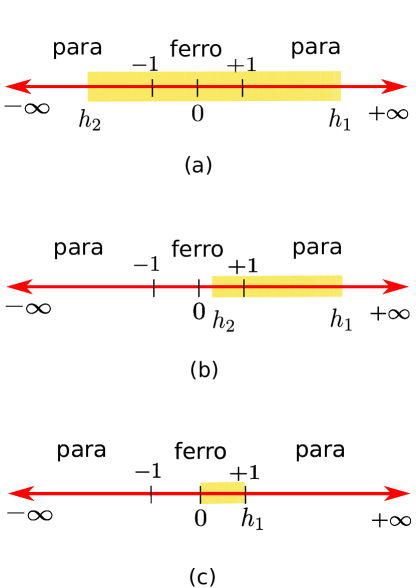
Figure 2: Schematic diagram showing the different classes of QEs considered below: (a) Para-Para QE, where the unitary strokes are between $h_{1}\gg 1$ and $h_{2}\ll-1$ (b) Para-Ferro QE with the unitary strokes between $h_{1}\gg 1$ and $0<h_{2}<1$ and (c) Critical-Ferro QE, where the unitary strokes are between $h_{1}\to 1$ and $h_{2}=0$. The regimes of operations are shown by the yellow highlights. The quantum critical points at $h=\pm J=\pm 1$ separate the paramagnetic phases ($|h|>1$) from Ferromagnetic phase ($|h|<1$).

We thus consider (see Fig. 2) (i) Para-Para QE when the WM crosses two critical points, (ii) Para-Ferro QE with one critical point crossed, (iii) Critical-Ferro QE, and (iv) Generalized QE, and start the discussion with the engine of the first type. Each of these engines bring out different features as we detail next.

IV.1 Para-Para QE

A Para-Para QE can be realized with $h_{1}\gg 1$ and $h_{2}\ll-1$. The work done in a Para-Para QE admits a closed form expression, which can directly be connected to Kibble-Zurek scaling. In order to explore the Kibble-Zurek scaling in heat engines, it is important that one of the unitary dynamics start from the ground state of the Hamiltonian. We choose the parameters of the relaxing bath such that it takes the system closest to its ground state. The unitary dynamics from $\bf D$ to $\bf A$ will then show the Kibble-Zurek scaling. For this, we fix $\mu_{\rm R}=1$ and $\mu_{\rm R}^{\prime}=0$, since it is the $\mu$ term which brings the system to the ground state for negative field values. We choose energizing bath $\mathcal{B}_{\rm E}$ parameters as $\mu_{\rm E}<1$ and $\mu_{\rm E}^{\prime}=1$. Also, we choose $h_{1}\gg 1$ and $h_{2}\ll-1$ so that both the critical points $h=\pm 1$ are crossed. The ground state for both the field values is paramagnetic where $c-$ particles are also the quasiparticles. This will help in getting closed analytical expressions for $\mathcal{Q}_{\rm in}$, $\mathcal{Q}_{\rm out}$ and work done, and finally their dependence on criticality.

IV.1.1 Analytical calculations

Our analytical expressions for the various energy values below are obtained for $h_{1}\gg 1$, $h_{2}\ll-1$, $|h_{1}|\gg|h_{2}|$. We further consider a high entropy steady state at B or $\tau_{1}$ small, or both, so that one can write the density matrix at $C$. We first note that the basis $|0,0\rangle,|1_{k},0\rangle,|0,1_{-k}\rangle,|1_{k},1_{-k}\rangle$ are also the eigen basis of the Hamiltonian for large $|h|$; see Eq. (30). To calculate energies $\mathcal{E}_{\rm B}$, $\mathcal{E}_{\rm C}$, $\mathcal{E}_{\rm D}$ and $\mathcal{E}_{\rm A}$, at ${\bf B}$, ${\bf C}$, ${\bf D}$ and ${\bf A}$ respectively, using Eq. (7), we need to write the density matrix at each of these points. One can see that at ${\bf B}$, when the system has reached its steady state after connecting to the energizing bath $\mathcal{B}_{\rm E}$ with $\mu=\mu_{\rm E}$ and $\mu^{\prime}=\mu_{\rm E}^{\prime}$, the density matrix takes the form

$$\rho_{k}^{\rm B}=\begin{bmatrix}P_{4}^{\rm B}&0&0&0\\ 0&P_{3}^{\rm B}&0&0\\ 0&0&P_{2}^{\rm B}&0\\ 0&0&0&P_{1}^{\rm B}\end{bmatrix},$$ (32)

where $P_{1}^{\rm B},P_{2}^{\rm B},P_{3}^{\rm B},P_{4}^{\rm B}$ are the populations in the energy levels $E_{1},E_{2},E_{3}$ and $E_{4}$ of the Hamiltonian with $E_{1}<E_{2}=E_{3}<E_{4}$ for $h_{1}\gg 1$. Clearly, the order reverses for $h\ll-1$. The symbol B in superscript represents point ${\bf B}$ of the cycle. We shall use the symbol D for quantities related to point ${\bf D}$ for similar reasons. These probabilities can be obtained using the steady state condition of the master equation which gives

$$\frac{P_{2}^{\rm B}}{P_{1}^{\rm B}}=\frac{P_{3}^{\rm B}}{P_{1}^{\rm B}}=\frac{P_{4}^{\rm B}}{P_{2}^{\rm B}}=\frac{P_{4}^{\rm B}}{P_{3}^{\rm B}}=\mu_{\rm E}$$ (33)

where $\mu_{\rm E}^{\prime}=1$ as discussed before. Also, from the normalisation condition we have

$$P_{1}^{\rm B}+P_{2}^{\rm B}+P_{3}^{\rm B}+P_{4}^{\rm B}=1.$$ (34)

From (33) and (34), we get the populations in the energy levels when connected to the ${\mathcal{B}_{\rm E}}$ as

$$P_{1}^{\rm B} = \frac{1}{(1+\mu_{\rm E})^{2}},$$

$$P_{2}^{\rm B} = P_{3}^{\rm B}=\frac{\mu_{\rm E}}{(1+\mu_{\rm E})^{2}},$$

$$P_{4}^{\rm B} = \frac{\mu_{\rm E}^{2}}{(1+\mu_{\rm E})^{2}}.$$ (35)

Using these expressions, we can write the steady state density matrix of the system at $\bf B$ in terms of $\mu_{\rm E}$. It is to be noted that the density matrix is independent of $k$ in these limits. As mentioned before, we choose an energizing bath which results in a high-entropy state at B, or small $\tau_{1}$, or both so that $\rho_{\rm C}=\rho_{\rm B}$. As shown in Appendix A the energy at $\bf B$ ($\mathcal{E}_{\rm B}$), and $\bf C$ ($\mathcal{E}_{\rm C}$) can now be written as

$$\mathcal{E}_{\rm B}=Lh_{1}\frac{\mu_{\rm E}-1}{\mu_{\rm E}+1},$$

$$\mathcal{E}_{\rm C}=Lh_{2}\frac{\mu_{\rm E}-1}{\mu_{\rm E}+1}.$$ (36)

Since the decay bath takes the system very close to the ground state $\mathcal{E}_{\rm D}=-L|h_{2}|$ for $h_{2}\ll-1$. We write $\mathcal{E}_{\rm A}$ as $\mathcal{E}_{\rm A}^{\rm G}+\mathcal{E}_{\rm ex,A}$ where $\mathcal{E}_{\rm A}^{\rm G}$ is the ground state energy corresponding to the Hamiltonian at $\bf A$ and is equal to $-Lh_{1}$. $\mathcal{E}_{\rm ex,A}$ is the excess energy, which will show the Kibble-Zurek scaling. The work done $\mathcal{W}$ by the system is $-(\mathcal{Q}_{\rm in}+\mathcal{Q}_{\rm out})$, which can be simplified using the above discussion, and can be written as

$$\mathcal{E}_{\rm ex,A} = \mathcal{W}+\frac{2L}{1+\mu_{\rm E}}(\mu_{\rm E}h_{1}-|h_{2}|)$$ (37)

$$\propto \tau_{2}^{-\frac{\nu d}{\nu z+1}}=\tau_{2}^{-\frac{1}{2}}$$

since $n_{\rm ex}\propto\mathcal{E}_{\rm ex,A}$ in the paramagnetic phase, and $\nu=z=1$ for transverse Ising model. We verify this scaling in Fig. 3, which establishes the novel relation (13) between the work done in a QE and the universal critical exponents of the quantum critical point crossed. For numerical calculations, the initial density matrix is evolved as per the Eq. (31) when connected to bath, whereas in the unitary stroke it is simply given by (6) The energies at A, B, C, D are calculated to obtain $\mathcal{Q}_{\rm in}$, $\mathcal{Q}_{\rm out}$, and the work done. This work done, upto an additive constant, shows the universal scaling as shown in Eq. (16), and is plotted in Fig. 3. We also show the efficiency of the engine as a function of $\tau_{2}$ in the inset of Fig 3 which approaches a constant value for large $\tau_{2}$.

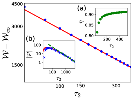
Figure 3: Work output showing universal Kibble-Zurek scaling in Para-Para QE. The points are the numerical values and red solid line corresponds to $\tau_{2}^{-1/2}$. For transverse Ising model, $d=\nu=z=1$. Inset (a): Variation of $\eta$ with $\tau_{2}$. (b) Variation of Power with $\tau_{2}$. The green dashed line corresponds to $1/\tau_{2}$ scaling, points represent numerical data and solid line is the analytical expression. The parameters used are: $L=100,h_{1}=70,h_{2}=-5,\tau_{1}=0.01,\mu_{\rm E}^{\prime}=1,\mu_{\rm E}=0.995,\mu_{\rm R}^{\prime}=0,\mu_{\rm R}=1$ with $\mathcal{W}_{\infty}=$-6481.205

.

To further characterize the performance, we consider the power as a function of $\tau_{2}$ in the inset (b) of Fig. 3. As discussed in section III.1, both analytical as well as numerical curves show a peak at $\tau_{2}=\tau_{\rm opt}$. The difference between the numerical data and the analytical result is mainly because the Kibble Zurek scaling, which also appears in the expression for power, is valid only for large $\tau_{2}$ whereas the peak occurs at smaller values. The analytical and numerical values of efficiency at maximum power, $\hat{\eta}$, are respectively given by 0.81 and 0.83, are thus in good agreement. The figure being a in log-log plot captures the $1/\tau_{2}$ behavior of power for large $\tau_{2}$ which can be explained using Eq. (17).

IV.2 Para-Ferro QE

Figure 4: Work output showing universal Kibble-Zurek scaling in Para-Ferro QE. The points are the numerical values and red solid line corresponds to $\tau_{2}^{-1/2}$. Inset (a): Variation of $\eta$ with $\tau_{2}$. (b) Variation of $\mathcal{P}$ with $\tau_{2}$. The green dashed line corresponds to $1/\tau_{2}$ scaling, points represent numerical data and solid line is the analytical expression. The parameters used are: $L=100,h_{1}=10,h_{2}=0,\tau_{1}=0.01,\mu_{\rm E}^{\prime}=1,\mu_{\rm E}=0.995$ with $\mathcal{W}_{\infty}=-899.995$.

We realize Para-Ferro QE by considering $h_{1}\gg 1$ and $0<h_{2}<1$, such that only the paramagnetic - ferromagnetic critical point is crossed during the unitary strokes. We consider an energizing bath of the form shown in Eq. (31), and a relaxing bath $\mathcal{B}_{\rm R}$ which takes the system close to its ground state. Similar to the previous case of Para-Para engine, the work done $\mathcal{W}$, up to some constant additive factor, will show Kibble-Zurek scaling, as long as the conditions given in Sec. III.1 are satisfied. This is presented in Fig. 4.

In order to understand the connection between excitations and engine parameters, we plot below $|W|$ as a function of $h_{2}$ in Fig. 5 We observe a decrease in power and work done as the critical point is approached, which can be attributed to the excitations produced near the critical point, tantamount to quantum friction. On the other hand, in absence of non-adiabatic excitations expected for slow quenches $\tau_{2}\to\infty$ and shortcuts to adiabaticity Hartmann et al. (2020), driving the quantum engine across a quantum critical point can boost the total work output.

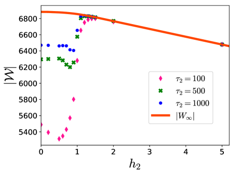
Figure 5: Work done as a function of $h_{2}$ for different $\tau$ values along with $W_{\infty}$, as defined in the main text. $\mathcal{W}$ improves as $\tau$ increases, or, when adiabaticity is increased. The parameters used are:$L=100,h_{1}=70,\tau_{1}=0.01,\mu_{\rm E}^{\prime}=1,\mu_{\rm E}=0.995$.

IV.3 Critical-Ferro QE

As described in section III.1, we now present the numerical results when $h_{1}$ is set close to its critical value of unity. During the stroke from D to A the transverse field is linearly varied from $h_{2}=0$ to a value close to its critical value of unity. As discussed in Ref. De Grandi et al. (2010); Fei et al. (2020), the scaling of excess energy gets modified. Putting $\nu=1$, $z=1$ and $d=1$ in Eq. (15) we get $\tau_{2}^{-1}$ as shown in Fig. 6, provided all the conditions of Sec. III.1 are satisfied.

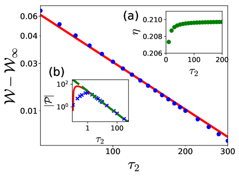
Figure 6: Work output showing modified Kibble-Zurek scaling when $h_{1}$ is close to the critical point. The points are the numerical values and red solid line corresponds to $\tau_{2}^{-1}$. Inset:(a) Variation of $\eta$ with $\tau_{2}$. (b) Variation of $\mathcal{P}$ with $\tau_{2}$ where points represent numerical data and solid line is the analytical expression. Also drawn is the green dashed line showing $1/\tau_{2}$ scaling. The parameters used are: $L=100,h_{1}=0.99,h_{2}=0.0,\tau_{1}=0.01,\mu_{\rm E}^{\prime}=1,\mu_{\rm E}=0.995$ with $\mathcal{W}_{\infty}=-26.532$.

IV.4 Generalized QE

Here we present the most general QE without any restrictions on the relaxing bath, i.e., without necessarily taking the WM to its ground state. In principle, Generalized QE can take any bath parameters and $h_{1}$, $h_{2}$, provided it works as an engine, but as we explain below, the analytical expressions are evaluated under certain conditions. We focus on elucidating how the engine parameters change as $h_{2}$ is varied across the critical point for fixed $h_{1}$ and other parameter values. With $h_{1}\gg 1$ and $h_{2}>0$, we choose the energizing bath $\mathcal{B}_{\rm E}$ parameters to be $\mu^{\prime}_{\rm E}=1$ and $\mu_{\rm E}<1$ and the relaxing bath $\mathcal{B}_{\rm R}$ parameters to be $\mu^{\prime}_{\rm R}=1$ and $\mu_{\rm R}<\mu_{\rm E}$. This set of parameters related to the relaxing bath will take the system to some steady state which is not the ground state at D. One can obtain analytical expressions along the same lines as in the para-para section, also presented in Appendix but with the condition that $\rho_{B}=\rho_{C}$ and $\rho_{D}=\rho_{A}$. This is true as long as the critical point is not crossed or $h_{2}>1$. The deviation between numerics and analytics start appearing when $h_{2}$ approaches the critical point.

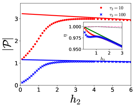
Figure 7: Variation of $|\mathcal{P}|$ as a function of $h_{2}$ for fixed $h_{1}$, $\mu_{\rm E}$, $\mu_{\rm R}$, but for different $\tau_{2}$ values. The points correspond to numerical values and solid lines to analytical. Inset: Variation of $\eta$ and $\eta_{\rm max}$ (black dotted line) as a function of $h_{2}$. $\eta_{\rm max}$ is calculated using Eq. (24) with $\nu=z=1$ for transverse Ising model. The maximum value of $\eta_{\rm max}$ is always less than unity as also confirmed by dashed-dotted line corresponding to $\eta=1$. The other parameters are: $L=100,h_{1}=70,\tau_{1}=0.1,\mu^{\prime}_{\rm E}=1,\mu_{\rm E}=0.995,\mu^{\prime}_{\rm R}=1,\mu_{\rm R}=0.95$.

We shall focus on the behavior of the QE power output $\mathcal{P}$ for different values of $h_{2}$. The final expressions in the limit of large $h_{1}$ and $h_{2}$ are:

$$\eta = 1-\frac{h_{2}}{h_{1}},$$ (38)

$$\mathcal{P} = -\frac{L(h_{1}-h_{2})}{\tau_{\rm total}}\left(\frac{\mu_{\rm E}-1}{\mu_{\rm E}+1}-\frac{\mu_{\rm R}-1}{\mu_{\rm R}+1}\right).$$ (39)

In Fig. 7, we present the behavior of power $\mathcal{P}$ as a function of $h_{2}$ for fixed $h_{1}$, $\mu_{\rm E}$, $\mu_{\rm R}$ $\tau_{1}$, and different $\tau_{2}$ values. Clearly, there is a better agreement between numerical and analytical values of $\mathcal{P}$ for larger $h_{2}$. Deviations between the two are more pronounced as the critical point is approached, as excitations generated with the crossing of the critical point are not included in the analytical calculations (38). The power $\mathcal{P}$ shows a sharp fall for a QE driven across the phase transition. This behavior can also be attributed to the excitations produced in the WM close to criticality, which in turn results in diminishing $\mathcal{Q}_{\rm in}$, and thus reduce the output power. We note that $|0,0\rangle,|1_{k},0\rangle,|0,1_{-k}\rangle,|1_{k},1_{-k}\rangle$ stop being eigenbasis of the WM for small $h_{2}$.

In the inset of Fig. 7, we present the behavior of efficiency as a function of $h_{2}$ for different $\tau_{2}$ values. As in the previous case, there is a good match between the analytical and numerical calculations when away from the QCP, in the paramagnetic phase. On the other hand, analytical calculations of Sec. IV.1.1 fail to explain the numerical results obtained close to the QCP and in the ordered ferromagnetic phase. As is expected from Eq. (38), the efficiency is independent of $\tau_{2}$ when the operation is confined inside the paramagnetic phase, for large $h_{1},h_{2}$. However, for a QE driven across a phase transition ($h_{1}>1,~{}h_{2}<1$), as shown in Fig. 7 (inset), the results can be expected to depend non-trivially on $\tau_{2}$, owing to the dependence of the non-adiabatic excitations on the rate of driving $\tau_{2}^{-1}$ across the QCP Zurek et al. (2005); Polkovnikov (2005); Dutta et al. (2015).

V Conclusion

We have studied the effect of quantum criticality in quantum thermodynamics, by considering a many-body quantum machine operating close to a phase transition. As a WM for the Otto cycle studied here, we have considered interacting Fermions coupled to local dissipative baths, which in the Fourier-transformed space, can be treated as non-interacting Fermions coupled to local non-interacting Fermionic dissipative baths. This property makes the setup analytically solvable in many regimes. Earlier studies on dynamics of closed many-body systems driven across a quantum critical point have shown the existence of universal finite-time scaling with the driving speed of different observables, including defect density Zurek et al. (2005); Polkovnikov (2005); Mukherjee et al. (2007) and its fluctuations del Campo (2018); Cui et al. (2020); Bando et al. (2020), and fidelity susceptibility De Grandi et al. (2010); Mukherjee et al. (2011), among other examples. Such finite time scaling can be justified from the diverging length and time scales close to a quantum critical point. In this work, we have shown for the first time the existence of such universality in quantum thermodynamics close to phase transitions, in the form of Kibble-Zurek scaling Zurek et al. (2005); Polkovnikov (2005) in the work output, and the operation of quantum engines close to criticality. Furthermore, we have derived a maximum efficiency bound $\eta_{\rm max}$, which scales with the dynamical critical exponent close to quantum criticality, and increases with increasing system size, thus showing the advantage of developing many-body quantum engines.

We have demonstrated these generic results using the model of Ising spin chain in presence of a transverse field. Our analytical and numerical results show that the work output inherits a Kibble-Zurek scaling form, up to an additive constant, for a quantum engine driven across quantum critical points ($h_{1}\gg 1$, $h_{2}\ll-1$ or $h_{1}\gg 1$, $-1<h_{2}<1$). By contrast, for a quantum engine confined to the paramagnetic phase, the power attains a maxima close to the QCP ($h_{1}\gg 1$, $h_{2}>1$), rapidly decreasing once the WM approaches the QCP ($h_{1}\gg 1$, $h_{2}\to 1^{+}$), diminishing close to zero when the efficiency is maximum. The loss of power in this case can be attributed to the generation of excitations close to quantum criticality.

While we have mainly focussed on Fermionic baths, our results can be expected to be valid for other kind of baths, as long as the conditions stated in Sec. III.1 are satisfied. We note that in this case the relaxing bath would be a thermal bath at absolute zero temperature, such that the WM reaches close to its ground state at the end of the non-unitary stroke C to D. Consequently, the efficiency of the quantum heat engine would be bounded by the Carnot limit of maximum efficiency, which in this case reduces to the trivial result $\eta\leq 1$. In addition, by considering thermal instead of Fermionic bath, our setting can be readily adapted to the characterization of quantum refrigerators.

The class of quantum machines studied here provides an opportunity to scale up quantum devices to the macroscopic regime, with a complete understanding of their performance. Experimental implementations can be envisioned in an optical lattice setup Schreiber et al. (2015). Our results should also be of relevance to the scaling of quantum machines using trapped ion chains as a working medium Roßnagel et al. (2016); Maslennikov et al. (2019); von Lindenfels et al. (2019) in which a quantum Ising chain can be emulated Friedenauer et al. (2008); Zhang et al. (2017); Bernien et al. (2017) and in which universal critical dynamics has been studied del Campo et al. (2010); Silvi et al. (2013, 2016), with experiments reported to date probing it in the classical regime Ejtemaee and Haljan (2013); Ulm et al. (2013); Pyka et al. (2013). Nuclear magnetic resonance experiments and nitrogen vacancy centers offer alternative platforms in which the quantum engines reported to date Peterson et al. (2019); Klatzow et al. (2019) can be scaled up considering quantum critical spin systems as working substance. Beyond specific implementations, our results advance the study of universal critical phenomena in quantum thermodynamics.

Appendix A Dynamics of the Working Medium

Para - Para engine

The density matrix at $\bf B$ for each $k$ mode takes the form given in Eq. (32) so that the energy is calculated as $\mathcal{E}_{\rm B}=\sum_{k}\text{Tr}[H(h_{1},k)\rho_{\rm B}]$. Therefore for each $k$ mode,

$H\rho_{\rm B}=$

$$\begin{split}\footnotesize{\begin{bmatrix}2(h_{1}+\cos k)&0&0&2\sin k\\ 0&0&0&0\\ 0&0&0&0\\ 2\sin k&0&0&-2(h_{1}+\cos k)\end{bmatrix}\begin{bmatrix}P_{4}^{\rm B}&0&0&0\\ 0&P_{3}^{\rm B}&0&0\\ 0&0&P_{2}^{\rm B}&0\\ 0&0&0&P_{1}^{\rm B}\end{bmatrix}}\end{split}$$ (40)

which gives

$$\text{Tr}[H\rho_{\rm B}] =2(h_{1}+\cos k)(P_{4}^{\rm B}-P_{1}^{\rm B})$$ (41)

$$=2(h_{1}+\cos k)\left(\frac{\mu_{\rm E}-1}{\mu_{\rm E}+1}\right).$$ (42)

For a system of size $L$, there are $L/2$ positive $k$ modes so that

$$\mathcal{E}_{\rm B} = \sum_{k}2(h_{1}+\cos k)\left(\frac{\mu_{\rm E}-1}{\mu_{\rm E}+1}\right)$$ (43)

$$= Lh_{1}\left(\frac{\mu_{\rm E}-1}{\mu_{\rm E}+1}\right).$$

Since the Hamiltonian is changed suddenly (small $\tau_{1}$) from $h_{1}$ to $h_{2}$, the density matrix is not able to evolve resulting to $\rho_{C}=\rho_{B}$ and thus energy at $\bf C$ $(\mathcal{E}_{\rm C})$ is

$$\mathcal{E}_{\rm C} = \sum_{k}2(h_{2}+\cos k)\left(\frac{\mu_{\rm E}-1}{\mu_{\rm E}+1}\right)$$ (44)

$$= Lh_{2}\left(\frac{\mu_{\rm E}-1}{\mu_{\rm E}+1}\right).$$

Since $\bf D$ is in the ground state, we have $\mathcal{E}_{\rm D}=-L|h_{2}|$. We write energy at $\bf A$ to be $\mathcal{E}_{\rm A}=\mathcal{E}_{\rm A}^{\rm G}+\mathcal{E}_{\rm ex,A}$ with $\mathcal{E}_{\rm A}^{\rm G}=-Lh_{1}$. This gives

$$\mathcal{Q}_{\rm in} =\mathcal{E}_{\rm B}-\mathcal{E}_{\rm A}$$ (45)

$$=\frac{2L\mu_{\rm E}h_{1}}{\mu_{\rm E}+1}-\mathcal{E}_{\rm ex,A}$$ (46)

and

$$\mathcal{Q}_{\rm out} = \mathcal{E}_{\rm D}-\mathcal{E}_{\rm C}$$ (47)

$$= \frac{-2L|h_{2}|}{\mu_{\rm E}+1}.$$

The work done, $\mathcal{W}=-(\mathcal{Q}_{\rm in}+\mathcal{Q}_{\rm out})$, is thus

$$\mathcal{W}=-\left(\frac{2L}{\mu_{\rm E}+1}(\mu_{\rm E}h_{1}-|h_{2}|)-\mathcal{E}_{\rm ex,A}\right)$$ (48)

or equivalently

$$\mathcal{W}+\frac{2L}{\mu_{\rm E}+1}(\mu_{\rm E}h_{1}-|h_{2}|)\propto\tau_{2}^{\frac{-\nu d}{1+\nu z}}.$$ (49)

Generalized QE

Clearly, there is no change in $\mathcal{E}_{\rm B}$ so that it is given by Eq. (43). For large $h_{2}$ with $h_{2}<h_{1}$, there will not be any population change in B to C, and hence the density matrix $\rho_{\rm B}$ will be same as $\rho_{\rm C}$ so that $\mathcal{E}_{\rm C}$ is also given by Eq. (44).

The energy at $\bf D$ would be different since the relaxing bath parameters are so chosen that it need not take the system to the ground state. It can be calculated as follows:

$$\mathcal{E}_{\rm D} =\sum_{k}\text{Tr}[H(h_{2},k)\rho_{\rm D}]$$ (50)

$$=\sum_{k}2(h_{2}+\cos k)(P_{4}^{\rm D}-P_{1}^{\rm D})$$ (51)

$$=\sum_{k}2(h_{2}+\cos k)\left(\frac{\mu_{\rm R}-1}{\mu_{\rm R}+1}\right)$$ (52)

$$=Lh_{2}\left(\frac{\mu_{\rm R}-1}{\mu_{\rm R}+1}\right).$$ (53)

Here, $\rho_{k}^{\rm D}$ would be similar to $\rho_{k}^{\rm B}$ as given in Eq. (32) with $\mu_{\rm E}$ replaced by $\mu_{\rm R}$. Similar calculations give

$$\mathcal{E}_{\rm A} =\sum_{k}\text{Tr}[H(h_{1},k)\rho_{\rm A}]$$ (54)

$$=Lh_{1}\left(\frac{\mu_{\rm R}-1}{\mu_{\rm R}+1}\right).$$ (55)

Now, the $\mathcal{Q}_{\rm in}$ and $\mathcal{Q}_{\rm out}$ for each $k$ mode is

$$\mathcal{Q}_{\rm in}(k) =2(h_{1}+\cos k)\left(\frac{\mu_{\rm E}-1}{\mu_{\rm E}+1}-\frac{\mu_{\rm R}-1}{\mu_{\rm R}+1}\right),$$ (56)

$$\mathcal{Q}_{\rm out}(k) =-2(h_{2}+\cos k)\left(\frac{\mu_{\rm E}-1}{\mu_{\rm E}+1}-\frac{\mu_{\rm R}-1}{\mu_{\rm R}+1}\right).$$ (57)

Let

$$\frac{\mu_{\rm E}-1}{\mu_{\rm E}+1}-\frac{\mu_{\rm R}-1}{\mu_{\rm R}+1}=\alpha.$$ (58)

Efficiency of the total system can be calculated using

$$\eta =\frac{\sum_{k}\mathcal{Q}_{\rm in}(k)+\sum_{k}\mathcal{Q}_{\rm out}(k)}{\sum_{k}\mathcal{Q}_{\rm in}(k)}$$ (59)

$$=\frac{2\alpha\sum_{k}[(h_{1}+\cos k)-(h_{2}+\cos k)]}{2\alpha\sum_{k}(h_{1}+\cos k)}$$ (60)

$$=\frac{\frac{L}{2}(h_{1}-h_{2})}{\frac{L}{2}h_{1}+\underbrace{\Sigma_{k}\cos k}}_{=0}$$ (61)

$$=1-\frac{h_{2}}{h_{1}}.$$ (62)

Power for the total system is defined as

$$\mathcal{P} =\frac{\text{net work done by the system}}{\text{total cycle time}}$$ (63)

$$=-\frac{2\alpha\sum_{k}[(h_{1}+\cos k)-(h_{2}+\cos k)]}{\tau_{\rm total}}$$ (64)

$$=-\frac{2\alpha(\frac{L}{2})(h_{1}-h_{2})}{\tau_{\rm total}}$$ (65)

$$=-\frac{L(h_{1}-h_{2})}{\tau_{\rm total}}\left(\frac{\mu_{\rm E}-1}{\mu_{\rm E}+1}-\frac{\mu_{\rm R}-1}{\mu_{\rm R}+1}\right).$$ (66)

References

- Roßnagel et al. (2016) Johannes Roßnagel, Samuel T. Dawkins, Karl N. Tolazzi, Obinna Abah, Eric Lutz, Ferdinand Schmidt-Kaler, and Kilian Singer, “A single-atom heat engine,” Science 352, 325–329 (2016).
- Maslennikov et al. (2019) Gleb Maslennikov, Shiqian Ding, Roland Hablützel, Jaren Gan, Alexandre Roulet, Stefan Nimmrichter, Jibo Dai, Valerio Scarani, and Dzmitry Matsukevich, “Quantum absorption refrigerator with trapped ions,” Nature Communications 10, 202 (2019).
- von Lindenfels et al. (2019) D. von Lindenfels, O. Gräb, C. T. Schmiegelow, V. Kaushal, J. Schulz, Mark T. Mitchison, John Goold, F. Schmidt-Kaler, and U. G. Poschinger, “Spin heat engine coupled to a harmonic-oscillator flywheel,” Phys. Rev. Lett. 123, 080602 (2019).
- Klatzow et al. (2019) James Klatzow, Jonas N. Becker, Patrick M. Ledingham, Christian Weinzetl, Krzysztof T. Kaczmarek, Dylan J. Saunders, Joshua Nunn, Ian A. Walmsley, Raam Uzdin, and Eilon Poem, “Experimental demonstration of quantum effects in the operation of microscopic heat engines,” Phys. Rev. Lett. 122, 110601 (2019).
- Peterson et al. (2019) John P. S. Peterson, Tiago B. Batalhão, Marcela Herrera, Alexandre M. Souza, Roberto S. Sarthour, Ivan S. Oliveira, and Roberto M. Serra, “Experimental characterization of a spin quantum heat engine,” Phys. Rev. Lett. 123, 240601 (2019).
- Gemmer et al. (2009) Jochen Gemmer, Mathias Michel, and Günter Mahler, Quantum thermodynamics: Emergence of thermodynamic behavior within composite quantum systems, Vol. 784 (Springer, 2009).
- Jaramillo et al. (2016) J Jaramillo, M Beau, and A del Campo, “Quantum supremacy of many-particle thermal machines,” New J. Phys. 18, 075019 (2016).
- Mukherjee et al. (2020) Victor Mukherjee, Abraham G. Kofman, and Gershon Kurizki, “Anti-zeno quantum advantage in fast-driven heat machines,” Communications Physics 3, 8 (2020).
- Kosloff and Rezek (2017) Ronnie Kosloff and Yair Rezek, “The quantum harmonic otto cycle,” Entropy 19 (2017), 10.3390/e19040136.
- Jaseem et al. (2020) Noufal Jaseem, Michal Hajdušek, Vlatko Vedral, Rosario Fazio, Leong-Chuan Kwek, and Sai Vinjanampathy, “Quantum synchronization in nanoscale heat engines,” Phys. Rev. E 101, 020201 (2020).
- Scully et al. (2003) M. O. Scully, M. S. Zubairy, G. S. Agarwal, and H. Waltherl, “Extracting work from a single heat bath via vanishing quantum coherence,” Science 299, 862 (2003).
- Roßnagel et al. (2014) J. Roßnagel, O. Abah, F. Schmidt-Kaler, K. Singer, and E. Lutz, “Nanoscale heat engine beyond the carnot limit,” Phys. Rev. Lett. 112, 030602 (2014).
- Gardas and Deffner (2015) Bartłomiej Gardas and Sebastian Deffner, “Thermodynamic universality of quantum carnot engines,” Phys. Rev. E 92, 042126 (2015).
- Niedenzu et al. (2018) Wolfgang Niedenzu, Victor Mukherjee, Arnab Ghosh, Abraham G. Kofman, and Gershon Kurizki, “Quantum engine efficiency bound beyond the second law of thermodynamics,” Nature Communications 9, 165 (2018).
- Elouard et al. (2017a) Cyril Elouard, David A. Herrera-Martí, Maxime Clusel, and Alexia Auffèves, “The role of quantum measurement in stochastic thermodynamics,” npj Quantum Information 3, 9 (2017a).
- Elouard et al. (2017b) Cyril Elouard, David Herrera-Martí, Benjamin Huard, and Alexia Auffèves, “Extracting work from quantum measurement in maxwell’s demon engines,” Phys. Rev. Lett. 118, 260603 (2017b).
- Cottet et al. (2017) Nathanaël Cottet, Sébastien Jezouin, Landry Bretheau, Philippe Campagne-Ibarcq, Quentin Ficheux, Janet Anders, Alexia Auffèves, Rémi Azouit, Pierre Rouchon, and Benjamin Huard, “Observing a quantum maxwell demon at work,” Proceedings of the National Academy of Sciences 114, 7561–7564 (2017), https://www.pnas.org/content/114/29/7561.full.pdf .
- Hofer et al. (2017) Patrick P. Hofer, Jonatan Bohr Brask, Martí Perarnau-Llobet, and Nicolas Brunner, “Quantum thermal machine as a thermometer,” Phys. Rev. Lett. 119, 090603 (2017).
- Bhattacharjee et al. (2020) Sourav Bhattacharjee, Utso Bhattacharya, Wolfgang Niedenzu, Victor Mukherjee, and Amit Dutta, “Quantum magnetometry using two-stroke thermal machines,” New Journal of Physics 22, 013024 (2020).
- Watanabe et al. (2017) Gentaro Watanabe, B. Prasanna Venkatesh, Peter Talkner, and Adolfo del Campo, “Quantum performance of thermal machines over many cycles,” Phys. Rev. Lett. 118, 050601 (2017).
- Uzdin et al. (2015) Raam Uzdin, Amikam Levy, and Ronnie Kosloff, “Equivalence of quantum heat machines, and quantum-thermodynamic signatures,” Phys. Rev. X 5, 031044 (2015).
- Hartmann et al. (2020) Andreas Hartmann, Victor Mukherjee, Wolfgang Niedenzu, and Wolfgang Lechner, “Many-body quantum heat engines with shortcuts to adiabaticity,” Phys. Rev. Research 2, 023145 (2020).
- Kim et al. (2011) Sang Wook Kim, Takahiro Sagawa, Simone De Liberato, and Masahito Ueda, “Quantum szilard engine,” Phys. Rev. Lett. 106, 070401 (2011).
- Bengtsson et al. (2018) J. Bengtsson, M. Nilsson Tengstrand, A. Wacker, P. Samuelsson, M. Ueda, H. Linke, and S. M. Reimann, “Quantum szilard engine with attractively interacting bosons,” Phys. Rev. Lett. 120, 100601 (2018).
- Zheng and Poletti (2015) Yuanjian Zheng and Dario Poletti, “Quantum statistics and the performance of engine cycles,” Phys. Rev. E 92, 012110 (2015).
- Hardal and Müstecaplıoğlu (2015) Ali Ü. C. Hardal and Özgür E. Müstecaplıoğlu, “Superradiant quantum heat engine,” Scientific Reports 5, 12953 EP – (2015).
- Yunger Halpern et al. (2019) Nicole Yunger Halpern, Christopher David White, Sarang Gopalakrishnan, and Gil Refael, “Quantum engine based on many-body localization,” Phys. Rev. B 99, 024203 (2019).
- Türkpençe et al. (2017) Deniz Türkpençe, Ferdi Altintas, Mauro Paternostro, and Özgür E. Müstecaplioğlu, “A photonic carnot engine powered by a spin-star network,” EPL (Europhysics Letters) 117, 50002 (2017).
- Deng et al. (2013) Jiawen Deng, Qing-hai Wang, Zhihao Liu, Peter Hänggi, and Jiangbin Gong, “Boosting work characteristics and overall heat-engine performance via shortcuts to adiabaticity: Quantum and classical systems,” Phys. Rev. E 88, 062122 (2013).
- del Campo et al. (2014) A. del Campo, J. Goold, and M. Paternostro, “More bang for your buck: Super-adiabatic quantum engines,” Sci. Rep. 4, 6208 (2014).
- Beau et al. (2016) Mathieu Beau, Juan Jaramillo, and Adolfo del Campo, “Scaling-up quantum heat engines efficiently via shortcuts to adiabaticity,” Entropy 18, 168 (2016).
- Funo et al. (2017) Ken Funo, Jing-Ning Zhang, Cyril Chatou, Kihwan Kim, Masahito Ueda, and Adolfo del Campo, “Universal work fluctuations during shortcuts to adiabaticity by counterdiabatic driving,” Phys. Rev. Lett. 118, 100602 (2017).
- del Campo et al. (2018) Adolfo del Campo, Aurélia Chenu, Shujin Deng, and Haibin Wu, “Friction-free quantum machines,” in Thermodynamics in the Quantum Regime: Fundamental Aspects and New Directions, edited by Felix Binder, Luis A. Correa, Christian Gogolin, Janet Anders, and Gerardo Adesso (Springer International Publishing, Cham, 2018) pp. 127–148.
- Deng et al. (2018) Shujin Deng, Aurélia Chenu, Pengpeng Diao, Fang Li, Shi Yu, Ivan Coulamy, Adolfo del Campo, and Haibin Wu, “Superadiabatic quantum friction suppression in finite-time thermodynamics,” Sci. Adv. 4 (2018), 10.1126/sciadv.aar5909.
- Diao et al. (2018) Pengpeng Diao, Shujin Deng, Fang Li, Shi Yu, Aurélia Chenu, Adolfo del Campo, and Haibin Wu, “Shortcuts to adiabaticity in fermi gases,” New J. Phys. 20, 105004 (2018).
- Sachdev (1999) S. Sachdev, Quantum Phase Transitions (Cambridge University Press, Cambridge, England, 1999).
- Polettini et al. (2015) M. Polettini, G. Verley, and M. Esposito, “Efficiency statistics at all times: Carnot limit at finite power,” Phys. Rev. Lett. 114, 050601 (2015).
- Campisi and Fazio (2016) M. Campisi and R. Fazio, “The power of a critical heat engine,” Nat. Comm. 7, 11895 (2016).
- Chen et al. (2019) Yang-Yang Chen, Gentaro Watanabe, Yi-Cong Yu, Xi-Wen Guan, and Adolfo del Campo, “An interaction-driven many-particle quantum heat engine and its universal behavior,” npj Quantum Information 5, 88 (2019).
- Geva and Kosloff (1992) Eitan Geva and Ronnie Kosloff, “A quantum‐mechanical heat engine operating in finite time. a model consisting of spin‐1/2 systems as the working fluid,” The Journal of Chemical Physics 96, 3054–3067 (1992), https://doi.org/10.1063/1.461951 .
- Quan et al. (2007) H. T. Quan, Yu-xi Liu, C. P. Sun, and Franco Nori, “Quantum thermodynamic cycles and quantum heat engines,” Phys. Rev. E 76, 031105 (2007).
- Batalhão et al. (2014) Tiago B. Batalhão, Alexandre M. Souza, Laura Mazzola, Ruben Auccaise, Roberto S. Sarthour, Ivan S. Oliveira, John Goold, Gabriele De Chiara, Mauro Paternostro, and Roberto M. Serra, “Experimental reconstruction of work distribution and study of fluctuation relations in a closed quantum system,” Phys. Rev. Lett. 113, 140601 (2014).
- Smith et al. (2018) Andrew Smith, Yao Lu, Shuoming An, Xiang Zhang, Jing-Ning Zhang, Zongping Gong, H T Quan, Christopher Jarzynski, and Kihwan Kim, “Verification of the quantum nonequilibrium work relation in the presence of decoherence,” New Journal of Physics 20, 013008 (2018).
- Azimi et al. (2014) M Azimi, L Chotorlishvili, S K Mishra, T Vekua, W Hübner, and J Berakdar, “Quantum otto heat engine based on a multiferroic chain working substance,” New Journal of Physics 16, 063018 (2014).
- Chotorlishvili et al. (2016) L. Chotorlishvili, M. Azimi, S. Stagraczyński, Z. Toklikishvili, M. Schüler, and J. Berakdar, “Superadiabatic quantum heat engine with a multiferroic working medium,” Phys. Rev. E 94, 032116 (2016).
- Niedenzu and Kurizki (2018) Wolfgang Niedenzu and Gershon Kurizki, “Cooperative many-body enhancement of quantum thermal machine power,” New Journal of Physics 20, 113038 (2018).
- Çakmak et al. (2016) Selçuk Çakmak, Ferdi Altintas, and Özgür E. Müstecaplioglu, “Lipkin-meshkov-glick model in a quantum otto cycle,” The European Physical Journal Plus 131, 197 (2016).
- Ma et al. (2017) Yu-Han Ma, Shan-He Su, and Chang-Pu Sun, “Quantum thermodynamic cycle with quantum phase transition,” Phys. Rev. E 96, 022143 (2017).
- Çakmak and Müstecaplıoğlu (2019) Baris Çakmak and Özgür E. Müstecaplıoğlu, “Spin quantum heat engines with shortcuts to adiabaticity,” Phys. Rev. E 99, 032108 (2019).
- Dorner et al. (2012) R. Dorner, J. Goold, C. Cormick, M. Paternostro, and V. Vedral, “Emergent thermodynamics in a quenched quantum many-body system,” Phys. Rev. Lett. 109, 160601 (2012).
- Nigro et al. (2019) Davide Nigro, Davide Rossini, and Ettore Vicari, “Scaling properties of work fluctuations after quenches near quantum transitions,” Journal of Statistical Mechanics: Theory and Experiment 2019, 023104 (2019).
- Bunder and McKenzie (1999) J. E. Bunder and Ross H. McKenzie, “Effect of disorder on quantum phase transitions in anisotropic xy spin chains in a transverse field,” Phys. Rev. B 60, 344–358 (1999).
- Lieb et al. (1961) Elliott Lieb, Theodore Schultz, and Daniel Mattis, “Two soluble models of an antiferromagnetic chain,” Annals of Physics 16, 407 – 466 (1961).
- Pfeuty (1970) Pierre Pfeuty, “The one-dimensional ising model with a transverse field,” Annals of Physics 57, 79 – 90 (1970).
- Dziarmaga (2010) J. Dziarmaga, “Dynamics of a quantum phase transition and relaxation to a steady state,” Advances in Physics 59, 1063 (2010).
- Dutta et al. (2015) A. Dutta, G. Aeppli, B. K. Chakrabarti, U. Divakaran, T. F. Rosenbaum, and D. Sen, Quantum phase transitions in transverse field spin models: from statistical physics to quantum information (Cambridge University Press, Cambridge, 2015).
- Kitaev (2006) Alexei Kitaev, “Anyons in an exactly solved model and beyond,” Annals of Physics 321, 2 – 111 (2006), january Special Issue.
- Chen and Nussinov (2008) Han-Dong Chen and Zohar Nussinov, “Exact results of the kitaev model on a hexagonal lattice: spin states, string and brane correlators, and anyonic excitations,” Journal of Physics A: Mathematical and Theoretical 41, 075001 (2008).
- Sengupta et al. (2008) K. Sengupta, Diptiman Sen, and Shreyoshi Mondal, “Exact results for quench dynamics and defect production in a two-dimensional model,” Phys. Rev. Lett. 100, 077204 (2008).
- Keck et al. (2017) M. Keck, S. Montangero, G. E. Santoro, R. Fazio, and D. Rossini, “Dissipation in adiabatic quantum computers: lessons from an exactly solvable model,” New Journal of Physics 19, 113029 (2017).
- Bandyopadhyay et al. (2018) Souvik Bandyopadhyay, Sudarshana Laha, Utso Bhattacharya, and Amit Dutta, “Exploring the possibilities of dynamical quantum phase transitions in the presence of a markovian bath,” Scientific Reports 8, 11921 (2018).
- Schreiber et al. (2015) Michael Schreiber, Sean S. Hodgman, Pranjal Bordia, Henrik P. Lüschen, Mark H. Fischer, Ronen Vosk, Ehud Altman, Ulrich Schneider, and Immanuel Bloch, “Observation of many-body localization of interacting fermions in a quasirandom optical lattice,” Science 349, 842–845 (2015).
- Mukherjee et al. (2016) V. Mukherjee, W. Niedenzu, A. G. Kofman, and G. Kurizki, “Speed and efficiency limits of multilevel incoherent heat engines,” Phys. Rev. E 94, 062109 (2016).
- Polkovnikov (2005) Anatoli Polkovnikov, “Universal adiabatic dynamics in the vicinity of a quantum critical point,” Phys. Rev. B 72, 161201 (2005).
- Zurek et al. (2005) Wojciech H. Zurek, Uwe Dorner, and Peter Zoller, “Dynamics of a quantum phase transition,” Phys. Rev. Lett. 95, 105701 (2005).
- Mukherjee et al. (2007) Victor Mukherjee, Uma Divakaran, Amit Dutta, and Diptiman Sen, “Quenching dynamics of a quantum spin- chain in a transverse field,” Phys. Rev. B 76, 174303 (2007).
- Deffner (2017) Sebastian Deffner, “Kibble-zurek scaling of the irreversible entropy production,” Phys. Rev. E 96, 052125 (2017).
- Damski and Zurek (2006) Bogdan Damski and Wojciech H. Zurek, “Adiabatic-impulse approximation for avoided level crossings: From phase-transition dynamics to landau-zener evolutions and back again,” Phys. Rev. A 73, 063405 (2006).
- Polkovnikov et al. (2011) Anatoli Polkovnikov, Krishnendu Sengupta, Alessandro Silva, and Mukund Vengalattore, “Colloquium: Nonequilibrium dynamics of closed interacting quantum systems,” Rev. Mod. Phys. 83, 863–883 (2011).
- del Campo and Zurek (2014) Adolfo del Campo and Wojciech H. Zurek, “Universality of phase transition dynamics: Topological defects from symmetry breaking,” International Journal of Modern Physics A 29, 1430018 (2014).
- Caneva et al. (2007) Tommaso Caneva, Rosario Fazio, and Giuseppe E. Santoro, “Adiabatic quantum dynamics of a random ising chain across its quantum critical point,” Phys. Rev. B 76, 144427 (2007).
- Cui et al. (2016) Jin-Ming Cui, Yun-Feng Huang, Zhao Wang, Dong-Yang Cao, Jian Wang, Wei-Min Lv, Le Luo, Adolfo del Campo, Yong-Jian Han, Chuan-Feng Li, and Guang-Can Guo, “Experimental trapped-ion quantum simulation of the kibble-zurek dynamics in momentum space,” Scientific Reports 6, 33381 (2016).
- Bando et al. (2020) Yuki Bando, Yuki Susa, Hiroki Oshiyama, Naokazu Shibata, Masayuki Ohzeki, Fernand o Javier Gómez-Ruiz, Daniel A. Lidar, Adolfo del Campo, Sei Suzuki, and Hidetoshi Nishimori, “Probing the Universality of Topological Defect Formation in a Quantum Annealer: Kibble-Zurek Mechanism and Beyond,” arXiv e-prints , arXiv:2001.11637 (2020), arXiv:2001.11637 [quant-ph] .
- De Grandi et al. (2010) C. De Grandi, V. Gritsev, and A. Polkovnikov, “Quench dynamics near a quantum critical point,” Phys. Rev. B 81, 012303 (2010).
- Fei et al. (2020) Zhaoyu Fei, Nahuel Freitas, Vasco Cavina, H. T. Quan, and Massimiliano Esposito, “Work statistics across a quantum phase transition,” Phys. Rev. Lett. 124, 170603 (2020).
- Kibble (1980) T.W.B. Kibble, “Some implications of a cosmological phase transition,” Physics Reports 67, 183 – 199 (1980).
- Zurek (1985) W. H. Zurek, “Cosmological experiments in superfluid helium?” Nature 317, 505–508 (1985).
- Zurek (1996) W. H. Zurek, “Cosmological experiments in condensed matter systems,” Phys. Rep. 276, 177 (1996).
- Hoyos et al. (2007) José A. Hoyos, Chetan Kotabage, and Thomas Vojta, “Effects of dissipation on a quantum critical point with disorder,” Phys. Rev. Lett. 99, 230601 (2007).
- Patanè et al. (2008) Dario Patanè, Alessandro Silva, Luigi Amico, Rosario Fazio, and Giuseppe E. Santoro, “Adiabatic dynamics in open quantum critical many-body systems,” Phys. Rev. Lett. 101, 175701 (2008).
- Dutta et al. (2016) Anirban Dutta, Armin Rahmani, and Adolfo del Campo, “Anti-kibble-zurek behavior in crossing the quantum critical point of a thermally isolated system driven by a noisy control field,” Phys. Rev. Lett. 117, 080402 (2016).
- Wang and Fazio (2020) Pei Wang and Rosario Fazio, “Dissipative phase transitions in the fully-connected ising model with -spin interaction,” (2020), arXiv:2008.10045 [cond-mat.quant-gas] .
- Sen et al. (2008) Diptiman Sen, K. Sengupta, and Shreyoshi Mondal, “Defect production in nonlinear quench across a quantum critical point,” Phys. Rev. Lett. 101, 016806 (2008).
- Breuer and Petruccione (2002) H. P. Breuer and F. Petruccione, The Theory of Open Quantum Systems (Oxford University Press, 2002).
- del Campo (2018) Adolfo del Campo, “Universal statistics of topological defects formed in a quantum phase transition,” Phys. Rev. Lett. 121, 200601 (2018).
- Cui et al. (2020) Jin-Ming Cui, Fernando Javier Gómez-Ruiz, Yun-Feng Huang, Chuan-Feng Li, Guang-Can Guo, and Adolfo del Campo, “Experimentally testing quantum critical dynamics beyond the kibble-zurek mechanism,” Communications Physics 3, 44 (2020).
- Mukherjee et al. (2011) Victor Mukherjee, Anatoli Polkovnikov, and Amit Dutta, “Oscillating fidelity susceptibility near a quantum multicritical point,” Phys. Rev. B 83, 075118 (2011).
- Friedenauer et al. (2008) A. Friedenauer, H. Schmitz, J. T. Glueckert, D. Porras, and T. Schaetz, “Simulating a quantum magnet with trapped?ions,” Nature Physics 4, 757–761 (2008).
- Zhang et al. (2017) J. Zhang, G. Pagano, P. W. Hess, A. Kyprianidis, P. Becker, H. Kaplan, A. V. Gorshkov, Z.-X. Gong, and C. Monroe, “Observation of a many-body dynamical phase transition with a 53-qubit quantum simulator,” Nature 551, 601–604 (2017).
- Bernien et al. (2017) Hannes Bernien, Sylvain Schwartz, Alexander Keesling, Harry Levine, Ahmed Omran, Hannes Pichler, Soonwon Choi, Alexander S. Zibrov, Manuel Endres, Markus Greiner, Vladan Vuletić, and Mikhail D. Lukin, “Probing many-body dynamics on a 51-atom quantum simulator,” Nature 551, 579–584 (2017).
- del Campo et al. (2010) A. del Campo, G. De Chiara, Giovanna Morigi, M. B. Plenio, and A. Retzker, “Structural defects in ion chains by quenching the external potential: The inhomogeneous kibble-zurek mechanism,” Phys. Rev. Lett. 105, 075701 (2010).
- Silvi et al. (2013) Pietro Silvi, Gabriele De Chiara, Tommaso Calarco, Giovanna Morigi, and Simone Montangero, “Full characterization of the quantum linear-zigzag transition in atomic chains,” Annalen der Physik 525, 827–832 (2013).
- Silvi et al. (2016) Pietro Silvi, Giovanna Morigi, Tommaso Calarco, and Simone Montangero, “Crossover from classical to quantum kibble-zurek scaling,” Phys. Rev. Lett. 116, 225701 (2016).
- Ejtemaee and Haljan (2013) S. Ejtemaee and P. C. Haljan, “Spontaneous nucleation and dynamics of kink defects in zigzag arrays of trapped ions,” Phys. Rev. A 87, 051401 (2013).
- Ulm et al. (2013) S. Ulm, J. Roßnagel, G. Jacob, C. Degünther, S. T. Dawkins, U. G. Poschinger, R. Nigmatullin, A. Retzker, M. B. Plenio, F. Schmidt-Kaler, and K. Singer, “Observation of the kibble-zurek scaling law for defect formation in ion crystals,” Nat. Comm. 4, 2290 (2013).
- Pyka et al. (2013) K. Pyka, J. Keller, H. L. Partner, R. Nigmatullin, T. Burgermeister, D. M. Meier, K. Kuhlmann, A. Retzker, M. B. Plenio, W. H. Zurek, A. del Campo, and T. E. Mehlstäubler, “Topological defect formation and spontaneous symmetry breaking in ion coulomb crystals,” Nat. Comm. 4, 2291 (2013).