Semi-supervised Disentanglement
with Independent Vector Variational Autoencoders

Supplementary Information for “Semi-supervised Disentanglement
with Independent Vector Variational Autoencoders”

Abstract

We aim to separate the generative factors of data into two latent vectors in a variational autoencoder. One vector captures class factors relevant to target classification tasks, while the other vector captures style factors relevant to the remaining information. To learn the discrete class features, we introduce supervision using a small amount of labeled data, which can simply yet effectively reduce the effort required for hyperparameter tuning performed in existing unsupervised methods. Furthermore, we introduce a learning objective to encourage statistical independence between the vectors. We show that (i) this vector independence term exists within the result obtained on decomposing the evidence lower bound with multiple latent vectors, and (ii) encouraging such independence along with reducing the total correlation within the vectors enhances disentanglement performance. Experiments conducted on several image datasets demonstrate that the disentanglement achieved via our method can improve classification performance and generation controllability.

1 Introduction

A desirably disentangled representation contains individual units, each corresponding to a single generative factor of data while being invariant to changes in other units (Bengio et al., 2013). Such interpretable and invariant properties lead to benefits in downstream tasks including image classification and generation (Kingma et al., 2014; Makhzani et al., 2016; Narayanaswamy et al., 2017; Zheng & Sun, 2019).

Variational autoencoders (VAEs) (Kingma & Welling, 2014) have been actively utilized for unsupervised disentanglement learning (Kim & Mnih, 2018; Chen et al., 2018; Esmaeili et al., 2019; Kumar et al., 2018; Gao et al., 2019; Burgess et al., 2017). To capture the generative factors that are assumed to be statistically independent, many studies have encouraged the independence of latent variables within a representation (Higgins et al., 2017; Kim & Mnih, 2018; Chen et al., 2018). Despite their promising results, the usage of only continuous variables frequently causes difficulty in the discovery of discrete factors (e.g., object categories).

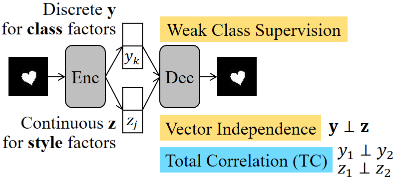
Figure 1: Proposed method with discrete and continuous random vectors, y and z. Weak classification supervision helps y capture discrete class factors. Our vector independence objective forces y and z to capture different information. Reducing this objective along with the TC improves disentanglement.

To address this issue, researchers have utilized discrete variables together with continuous variables to separately capture discrete and continuous factors (Dupont, 2018; Kingma et al., 2014) and trained their models by maximizing the evidence lower bound (ELBO). In this paper, we show that the ability of disentanglement in their models is derived from not only using the two types of variables but also encouraging several sources of disentanglement. We expose these sources by decomposing the ELBO.

Unsupervised learning with discrete and continuous variables is difficult, because continuous units with a large informational capacity often store all information, causing discrete units to store nothing and be neglected by models (Dupont, 2018). Previously, this issue was mostly solved using hyperparameter-sensitive capacity controls (Dupont, 2018) or additional steps for inferring discrete features during training (Jeong & Song, 2019). In contrast, we simply inject weak supervision with a few class labels and effectively resolve the difficulty in learning of discrete variables. Locatello et al. (2019) also suggested the exploitation of available supervision for improving disentanglement.

We introduce a semi-supervised disentanglement learning method, which is shown in Figure 1. A VAE was used to extract two feature vectors: one containing discrete variables to capture class factors and the other vector containing continuous variables to capture style factors. The contributions of this work to the relevant field of study are as follows:

• We introduce the vector independence objective that measures the statistical independence between latent vectors in VAEs and enables different vectors to store different information. We name our model an Independent Vector VAE (IV-VAE).

• We decompose the ELBO containing multiple latent vectors to reveal the vector independence term along with well-known total correlation (TC) terms that measure independence between the variables within the vectors. We show that these terms are the sources of disentanglement in jointly learning discrete and continuous units.

• We introduce supervision with a small number of class labels, significantly reducing the difficulty in learning discrete class features.

• We empirically show that our method enhances disentanglement learning on several image datasets, positively affecting the classification and controllable generation.

The supplementary material includes derivation details and additional results, and the sections are indicated with S (e.g., Section S1).

2 Related Work: Disentanglement Learning with VAEs

A $J$-dimensional random vector, $\textbf{z}=[z_{1},...,z_{J}]^{T}$, consists of scalar-valued random variables, $\{z_{j}\}$. Previous methods have encouraged independence between variables, whereas our method encourages independence between vectors (by introducing another vector, y) along with independence between the variables within the vectors.

2.1 Promoting Independence of Continuous Variables

Given dataset $D=\{\textbf{x}^{(1)},...,\textbf{x}^{(N)}\}$ containing $N$ i.i.d. samples of random vector x, a VAE learns latent vector z involved in the data generation process. The VAE consists of encoder $q_{\phi}(\textbf{z}|\textbf{x}^{(n)})$ and decoder $p_{\theta}(\textbf{x}^{(n)}|\textbf{z})$ trained by maximizing the ELBO on $\mathbb{E}_{q(\textbf{x})}\big{[}\log p_{\theta}(\textbf{x}^{(n)})\big{]}$, where the empirical distribution is represented as $q(\textbf{x})=\frac{1}{N}\sum\nolimits_{n=1}^{N}\delta(\textbf{x}-\textbf{x}^{(\textit{n})})$. The training objective consists of the reconstruction term and the KL divergence from the prior to individual posteriors:

$$\mathcal{L}^{z}_{\beta}=\mathbb{E}_{q(\textbf{x})}\Big{[}\mathbb{E}_{q_{\phi}(\textbf{z}|\textbf{x})}\big{[}\log p_{\theta}(\textbf{x}|\textbf{z})\big{]}\Big{]}-\beta\mathcal{L}^{z}_{KL}$$ (1)

$$\mathcal{L}^{z}_{KL}=\mathbb{E}_{q(\textbf{x})}\Big{[}\textrm{D}_{\textrm{KL}}\big{(}q_{\phi}(\textbf{z}|\textbf{x})||p(\textbf{z})\big{)}\Big{]},$$ (2)

where $\beta=1$ and $\beta>1$ in (1) represent the vanilla VAE and $\beta$-VAE (Higgins et al., 2017) objectives, respectively. Under factorized prior $p(\textbf{z})=\prod\nolimits_{j}p(z_{j})$ (e.g., $N(\textbf{0},\textbf{I})$), the $\beta$-VAE enhances the independence of latent variables, leading to disentanglement.

To understand the disentangling mechanism in VAEs, the KL term (2) was decomposed into (3) in (Hoffman & Johnson, 2016) and further into (4) under the factorized prior in (Chen et al., 2018):

$$\mathcal{L}^{z}_{KL}=I_{q_{\phi}}(\textbf{z};\textbf{x})+\textrm{D}_{\textrm{KL}}\big{(}q_{\phi}(\textbf{z})||p(\textbf{z})\big{)}$$ (3)

$$\mathcal{L}^{z}_{KL}=I_{q_{\phi}}(\textbf{z};\textbf{x})+\textrm{D}_{\textrm{KL}}\Big{(}q_{\phi}(\textbf{z})||\prod\nolimits_{j}q_{\phi}(z_{j})\Big{)}+\mathcal{L}^{z}_{Reg},$$ (4)

where $q_{\phi}(\textbf{z})=\int_{\textbf{x}}q_{\phi}(\textbf{z}|\textbf{x})q(\textbf{x})d\textbf{x}=\frac{1}{N}\sum\nolimits_{n=1}^{N}q_{\phi}(\textbf{z}|\textbf{x}^{(\textit{n})})$ is the aggregate posterior (Makhzani et al., 2016) that describes the latent structure for all data samples, $I_{q_{\phi}}(\textbf{z};\textbf{x})=\textrm{D}_{\textrm{KL}}\big{(}q_{\phi}(\textbf{z},\textbf{x})||q_{\phi}(\textbf{z})q(\textbf{x})\big{)}$ is the mutual information (MI) between the data and latent vectors under empirical distribution $q_{\phi}(\textbf{z}|\textbf{x})q(\textbf{x})$, and $\mathcal{L}^{z}_{Reg}=\sum\nolimits_{j}\textrm{D}_{\textrm{KL}}\big{(}q_{\phi}(z_{j})||p(z_{j})\big{)}$ is the regularization term for penalizing individual latent dimensions that excessively differ from their priors.

The second term in (4) represents the TC (Watanabe, 1960) that measures the statistical dependency of more than two random variables. Kim & Mnih (2018) and Chen et al. (2018) argued that (i) $\beta$-VAEs heavily penalize the MI term, $I_{q_{\phi}}(\textbf{z};\textbf{x})$, along with the other terms, causing z to be less informative about x, and (ii) the TC term is the source of disentanglement and thus should be strongly penalized. To address these issues, Kim & Mnih (2018) proposed the FactorVAE by adding the TC term to the vanilla VAE objective, and Chen et al. (2018) proposed the $\beta$-TCVAE by separately controlling the three terms in (4) using individual weights.

The previous methods (Higgins et al., 2017; Kim & Mnih, 2018; Chen et al., 2018) learned disentangled representations by encouraging the independence of continuous variables. They primarily employed Gaussian distributions for variational posteriors and consequently focused on modeling continuous generative factors. However, most datasets naturally contain discrete factors of variation (e.g., object classes), which these methods frequently fail to capture. We address this issue by incorporating discrete random variables and further enhance the disentanglement by promoting the independence between one set of discrete variables and another set of continuous variables.

2.2 Utilizing Discrete and Continuous Variables

To separately capture discrete and continuous factors, researchers have proposed the simultaneous utilization of discrete and continuous variables, which are stored in two latent vectors, y and z, respectively. By introducing joint prior $p(\textbf{y},\textbf{z})$, approximate posterior $q_{\phi}(\textbf{y},\textbf{z}|\textbf{x})$, and likelihood $p_{\theta}(\textbf{x}|\textbf{y},\textbf{z})$, the ELBO containing the reconstruction and KL terms becomes (see Section S1 for the derivation)

$$\mathcal{L}^{y,z}_{\beta}=\mathbb{E}_{q(\textbf{x})}\Big{[}\mathbb{E}_{q_{\phi}(\textbf{y},\textbf{z}|\textbf{x})}\big{[}\log p_{\theta}(\textbf{x}|\textbf{y},\textbf{z})\big{]}\Big{]}-\beta\mathcal{L}^{y,z}_{KL},$$ (5)

$$\mathcal{L}^{y,z}_{KL}=\mathbb{E}_{q(\textbf{x})}\Big{[}\textrm{D}_{\textrm{KL}}\big{(}q_{\phi}(\textbf{y},\textbf{z}|\textbf{x})||p(\textbf{y},\textbf{z})\big{)}\Big{]}.$$ (6)

By assuming factorized prior $p(\textbf{y},\textbf{z})=p(\textbf{y})p(\textbf{z})$, the KL can be decomposed depending on the factorized form of $q_{\phi}(\textbf{y},\textbf{z}|\textbf{x})$; Kingma et al. (2014) assumed $q_{\phi}(\textbf{y}|\textbf{x})q_{\phi}(\textbf{z}|\textbf{y},\textbf{x})$, and Dupont (2018) assumed $q_{\phi}(\textbf{y}|\textbf{x})q_{\phi}(\textbf{z}|\textbf{x})$ to derive

$$\begin{split}\mathcal{L}^{y,z}_{KL}=&\;\mathbb{E}_{q(\textbf{x})}\Big{[}\textrm{D}_{\textrm{KL}}\big{(}q_{\phi}(\textbf{y}|\textbf{x})||p(\textbf{y})\big{)}\\ &+\textrm{D}_{\textrm{KL}}\big{(}q_{\phi}(\textbf{z}|\textbf{x})||p(\textbf{z})\big{)}\Big{]}\end{split}.$$ (7)

In contrast, we decompose the KL term (6) to reveal the existence of the vector independence term between y and z as well as the TC terms within the vectors (see our decomposition in (11)). Moreover, our method explicitly encourages the vector independence term while not penalizing the latent-data MI terms, $I_{q_{\phi}}(\textbf{y};\textbf{x})$ and $I_{q_{\phi}}(\textbf{z};\textbf{x})$, to obtain disentangled informative features. We show that our method outperforms the $\beta$-VAE (Higgins et al., 2017) and its variant (Dupont, 2018), which strongly penalize the KL term (7) and consequently minimize the latent-data MI terms.

In addition, unsupervised learning with discrete and continuous variables often causes the discrete units to capture less information and be discarded by the model (Dupont, 2018) because of a larger informational capacity of continuous units than that of discrete units. To address this issue, existing unsupervised methods involve sophisticated hyperparameter tunings or additional computations. For example, Dupont (2018) modified (7) using capacity control terms separately for discrete and continuous units, and Jeong & Song (2019) proposed an alternating optimization between inferring probable discrete features and updating the encoder. In contrast, we introduce weak classification supervision to guide the encoder to store class factors in discrete units; this method simply but significantly reduces the effort needed for designing inference steps.

3 Proposed Approach

The problem scenario is identical to that described in Section 2.2, with discrete random vector $\textbf{y}\in{\rm I\!R}^{K}$ for capturing class factors and continuous random vector $\textbf{z}\in{\rm I\!R}^{J}$ for capturing style factors. First, we show that the ELBO can be decomposed into the proposed vector independence term and the others. Then, we present our semi-supervised learning (SSL) strategy.

3.1 Learning of Independent Latent Vectors

3.1.1 Vector Independence Objective

Assuming the conditional independence of $q_{\phi}(\textbf{y},\textbf{z}|\textbf{x})=q_{\phi}(\textbf{y}|\textbf{x})q_{\phi}(\textbf{z}|\textbf{x})$, an encoder produces the parameters for variational posteriors $q_{\phi}(\textbf{y}|\textbf{x}^{(\textit{n})})$ and $q_{\phi}(\textbf{z}|\textbf{x}^{(\textit{n})})$, for the n-th sample, $\textbf{x}^{(\textit{n})}$. The aggregate posteriors that capture the entire latent space under data distribution $q(\textbf{x})$ are defined as $q_{\phi}(\textbf{z})=\frac{1}{N}\sum\nolimits_{n=1}^{N}q_{\phi}(\textbf{z}|\textbf{x}^{(\textit{n})})$, $q_{\phi}(\textbf{y})=\frac{1}{N}\sum\nolimits_{n=1}^{N}q_{\phi}(\textbf{y}|\textbf{x}^{(\textit{n})})$, and

$$q_{\phi}(\textbf{y},\textbf{z})=\mathbb{E}_{q(\textbf{x})}\big{[}q_{\phi}(\textbf{y},\textbf{z}|\textbf{x})\big{]}=\frac{1}{N}\sum_{n=1}^{N}q_{\phi}(\textbf{y},\textbf{z}|\textbf{x}^{(\textit{n})}),$$ (8)

where $q_{\phi}(\textbf{y},\textbf{z}|\textbf{x})$ is computed using its decomposition form. Then, we define our vector independence objective as the MI between the two vectors that measures their statistical dependency:

$$\mathcal{L}^{y,z}_{VecIdp}=\textrm{D}_{\textrm{KL}}\big{(}q_{\phi}(\textbf{y},\textbf{z})||q_{\phi}(\textbf{y})q_{\phi}(\textbf{z})\big{)}.$$ (9)

Thr reduction of this term can enforce y and z to capture different semantics. Here, we emphasize that our method is applicable to cases with multiple L latent vectors by extending (9) to $\textrm{D}_{\textrm{KL}}\big{(}q_{\phi}(\textbf{z}_{1},...,\textbf{z}_{L})||\prod\nolimits_{l=1}^{L}q_{\phi}(\textbf{z}_{l})\big{)}$, which has a form similar to the TC computed over the variables (i.e., $\textrm{D}_{\textrm{KL}}\big{(}q_{\phi}(\textbf{z})||\prod\nolimits_{j=1}^{J}q_{\phi}(z_{j})\big{)}$) but is computed over the vectors. The relationship between the TC and the vector independence term is similar to that between the objectives of independent component analysis (ICA; Jutten & Herault (1991); Amari et al. (1996)) and independent vector analysis (IVA; Kim et al. (2006b, a)).

3.1.2 Our ELBO Decomposition

Chen et al. (2018) showed that the TC term measuring the dependency between latent variables (i) exists in the decomposion of the ELBO containing a single latent vector, z, and (ii) is a source of disentanglement in VAEs. Similarly, we reveal that the vector independence term (i) exists in the decomposition of the ELBO containing two latent vectors, y and z, and (ii) is another source of disentanglement.

Concretely, we decompose the KL term (6) of the ELBO into (10) under $p(\textbf{y},\textbf{z})=p(\textbf{y})p(\textbf{z})$ and further into (11) under $p(\textbf{y})=\prod\nolimits_{k}p(y_{k})$ and $p(\textbf{z})=\prod\nolimits_{j}p(z_{j})$:

$$\begin{split}\mathcal{L}^{y,z}_{KL}=&\;I_{q_{\phi}}(\textbf{y},\textbf{z};\textbf{x})+\textrm{D}_{\textrm{KL}}\big{(}q_{\phi}(\textbf{y},\textbf{z})||q_{\phi}(\textbf{y})q_{\phi}(\textbf{z})\big{)}\\ &+\textrm{D}_{\textrm{KL}}\Big{(}q_{\phi}(\textbf{y})||p(\textbf{y})\Big{)}+\textrm{D}_{\textrm{KL}}\Big{(}q_{\phi}(\textbf{z})||p(\textbf{z})\Big{)}\end{split}$$ (10)

$$\begin{split}\mathcal{L}^{y,z}_{KL}=&\;I_{q_{\phi}}(\textbf{y},\textbf{z};\textbf{x})+\textrm{D}_{\textrm{KL}}\big{(}q_{\phi}(\textbf{y},\textbf{z})||q_{\phi}(\textbf{y})q_{\phi}(\textbf{z})\big{)}\\ &+\textrm{D}_{\textrm{KL}}\Big{(}q_{\phi}(\textbf{y})||\prod\nolimits_{k}q_{\phi}(y_{k})\Big{)}+\mathcal{L}^{y}_{Reg}\\ &+\textrm{D}_{\textrm{KL}}\Big{(}q_{\phi}(\textbf{z})||\prod\nolimits_{j}q_{\phi}(z_{j})\Big{)}+\mathcal{L}^{z}_{Reg}\end{split},$$ (11)

where $I_{q_{\phi}}(\textbf{y},\textbf{z};\textbf{x})=\textrm{D}_{\textrm{KL}}\big{(}q_{\phi}(\textbf{y},\textbf{z},\textbf{x})||q_{\phi}(\textbf{y},\textbf{z})q(\textbf{x})\big{)}$ is the MI between x and latent vectors y and z, and $\mathcal{L}^{y}_{Reg}=\sum\nolimits_{k}\textrm{D}_{\textrm{KL}}\big{(}q_{\phi}(y_{k})||p(y_{k})\big{)}$ and $\mathcal{L}^{z}_{Reg}=\sum\nolimits_{j}\textrm{D}_{\textrm{KL}}\big{(}q_{\phi}(z_{j})||p(z_{j})\big{)}$ are the dimension-wise regularization terms. The derivation from (10) to (11) is motivated by that from (3) to (4). See Section S2 for the derivation details.

As suggested by Kim & Mnih (2018) and Chen et al. (2018), data-latent MI $I_{q_{\phi}}(\textbf{y},\textbf{z};\textbf{x})$ is not penalized during training so as to allow the latent vectors to capture data information. The second term in the RHS is our vector independence objective, and the third and fifth terms are the TC terms for the variables in y and z, respectively. We empirically show that simultaneously reducing these three terms provides better disentanglement compared to penalizing only the TC terms without considering the vector independence. The regularization terms, $\mathcal{L}^{y}_{Reg}$ and $\mathcal{L}^{z}_{Reg}$, forbid individual latent variables from deviating largely from the priors.

A concurrent work (Esmaeili et al., 2019) introduced a decomposition similar to our result in (11). Their derivation was initiated by augmenting the ELBO with a data entropy term (i.e., $-\mathbb{E}_{q(\textbf{x})}\big{[}\log q(\textbf{x})\big{]}$). In contrast to our method, their method with discrete and continuous units uses purely unsupervised learning, which often causes the discrete units to be ignored by the model.

3.1.3 Relationship between the Vector Independence Objective and TC

Here, we investigate the relationship between vector independence objective $\mathcal{L}^{y,z}_{VecIdp}$ (9) and the following TC terms:

$$\begin{split}&\mathcal{L}^{y}_{TC}=\textrm{D}_{\textrm{KL}}\Big{(}q_{\phi}(\textbf{y})||\prod\nolimits_{k}q_{\phi}(y_{k})\Big{)}\quad\textrm{and}\quad\\ &\mathcal{L}^{z}_{TC}=\textrm{D}_{\textrm{KL}}\Big{(}q_{\phi}(\textbf{z})||\prod\nolimits_{j}q_{\phi}(z_{j})\Big{)}\end{split}$$ (12)

$$\mathcal{L}^{y,z}_{TC}=\textrm{D}_{\textrm{KL}}\Big{(}q_{\phi}(\textbf{y},\textbf{z})||\prod\nolimits_{k}q_{\phi}(y_{k})\prod\nolimits_{j}q_{\phi}(z_{j})\Big{)}.$$ (13)

(12) measures the independence of the variables within each vector (hereafter called the “separate” TC). In addition, (13) simultaneously considers the variables in y and z (hereafter called the “collective” TC), and it can be viewed as the TC on concatenated vector $\textbf{h}=[$y$;\,$z$]$ (i.e., $\textrm{D}_{\textrm{KL}}\big{(}q_{\phi}(\textbf{h})||\prod\nolimits_{i}q_{\phi}(h_{i})\big{)}$).

We introduce two relationships. First, perfectly penalized collective TC indicates perfect vector independence:

$$\mathcal{L}^{y,z}_{TC}=0\;\Rightarrow\;\mathcal{L}^{y}_{TC}=\mathcal{L}^{z}_{TC}=\mathcal{L}^{y,z}_{VecIdp}=0$$ (14)

by letting $q_{\phi}(\textbf{z})=\prod\nolimits_{j}q_{\phi}(z_{j})$ and $q_{\phi}(\textbf{y})=\prod\nolimits_{k}q_{\phi}(y_{k})$. In this case, the vector independence objective would be naturally satisfied, resulting in unnecessary optimization. However, this case is rare because of the existence of other loss terms (e.g., a reconstruction term) that often prevent the collective TC from being zero. Furthermore, under the factorized prior, the perfectly penalized TC may be undesirable because it could imply the occurrence of posterior collapse (i.e., learning a trivial posterior that collapses to the prior and fails to capture data features). We present the experimental setup and results regarding this relationship in Sections S5 and S6.

Second, perfect vector independence does not ensure that all variables within and between the vectors are perfectly independent, i.e., $\mathcal{L}^{y,z}_{VecIdp}=0\;\nRightarrow\;\mathcal{L}^{y}_{TC}=\mathcal{L}^{z}_{TC}=\mathcal{L}^{y,z}_{TC}=0$. However, perfect vector independence ensures that the collective TC is the sum of the two separate TCs, i.e., $\mathcal{L}^{y,z}_{VecIdp}=0\;\Rightarrow\;\mathcal{L}^{y,z}_{TC}=\mathcal{L}^{y}_{TC}+\mathcal{L}^{z}_{TC}$ (see Section S3 for the derivation).

3.2 Semi-supervised Learning (SSL)

A weak classification supervision guides y to suitably represent discrete class factors. In addition, our vector independence objective further enforces y and z to capture different types of information. In our experiments, we simplify the problem setup by assuming that a given dataset involves a single classification task with $C$ classes. This enabled us to design $\textbf{y}\in{\rm I\!R}^{K}$ as a single categorical variable, $y\in\{1,...,C\}$, where $K=1$. We represent $y$ as a $C$-dimensional one-hot vector. For $\textbf{z}\in{\rm I\!R}^{J}$, we assume the existence of multiple style factors and expect each factor to be captured by each variable, $z_{j}$, within z.

The training image dataset consists of labeled set $L=\{(\textbf{x}^{(1)},t^{(1)}),...,(\textbf{x}^{(N_{L})},t^{(N_{L})})\}$, where the $n$-th image, $\textbf{x}^{(n)}$, is paired with the corresponding class label, $t^{(n)}\in\{1,...,C\}$, and unlabeled set $U=\{\textbf{x}^{(1)},...,\textbf{x}^{(N_{U})}\}$. Here, $N_{L}$ and $N_{U}$ are the numbers of samples in datasets $L$ and $U$, respectively, and $N_{L}\ll N_{U}$. The empirical data distributions over $L$ and $U$ are denoted by $q^{L}(\textbf{x},t)$ and $q^{U}(\textbf{x})$, respectively.

3.2.1 Semi-supervised Learning Objective

To update encoder parameter $\phi$ and decoder parameter $\theta$, the objectives for the labeled and unlabeled sets are given as

$$\mathcal{J}^{L}(\phi,\theta)=\mathcal{J}_{recon}^{L}(\phi,\theta)+\mathcal{J}_{cls}(\phi)-\mathcal{J}^{Both}(\phi)$$ (15)

$$\mathcal{J}^{U}(\phi,\theta)=\mathcal{J}_{recon}^{U}(\phi,\theta)-\mathcal{J}^{Both}(\phi).$$ (16)

For the following reconstruction terms, we use true label $t$ for $L$ and inferred feature $y$ for $U$. This strategy helps the decoder accurately recognize one-hot class vectors.

$$\mathcal{J}_{recon}^{L}(\phi,\theta)=\mathbb{E}_{q^{L}(\textbf{x},t)}\Big{[}\mathbb{E}_{q_{\phi}(\textbf{z}|\textbf{x})}\big{[}\log p_{\theta}(\textbf{x}|t,\textbf{z})\big{]}\Big{]}$$ (17)

$$\mathcal{J}_{recon}^{U}(\phi,\theta)=\mathbb{E}_{q^{U}(\textbf{x})}\Big{[}\mathbb{E}_{q_{\phi}(y,\textbf{z}|\textbf{x})}\big{[}\log p_{\theta}(\textbf{x}|y,\textbf{z})\big{]}\Big{]}$$ (18)

We compute the classification term for $L$ as

$$\mathcal{J}_{cls}(\phi)=\alpha\,\mathbb{E}_{q^{L}(\textbf{x},t)}\Big{[}\mathbb{I}(y=t)\log q_{\phi}(y|\textbf{x})\Big{]},$$ (19)

where hyper-parameter $\alpha$ controls the effect of discriminative learning. With scaling constant $\rho$, we set $\alpha=\rho\frac{N_{L}+N_{U}}{N_{L}}$ (Kingma et al., 2014; Maaløe et al., 2016).

Next, we introduce the following commonly used objective for $L$ and $U$ to learn disentangled features and regularize the encoder:

$$\begin{split}\mathcal{J}^{Both}(\phi)=&\;\lambda\,\mathcal{L}^{y,z}_{VecIdp}(\phi)+\gamma_{y}\,\mathcal{L}^{y}_{Reg}(\phi)\\ &+\beta_{z}\,\mathcal{L}^{z}_{TC}(\phi)+\gamma_{z}\,\mathcal{L}^{z}_{Reg}(\phi).\end{split}$$ (20)

This is identical to applying individual loss weights to the vector independence, TC, and dimension-wise regularization terms in our KL decomposition (11). Here, the expectation over the empirical distribution, i.e., $\mathbb{E}_{q^{U}(\textbf{x})}[\cdot]$ or $\mathbb{E}_{q^{L}(\textbf{x},t)}[\cdot]$, is included in computing the aggregated posteriors, $q_{\phi}($z$)$ and $q_{\phi}(y)$. Note that $\mathcal{L}^{y}_{TC}$ disappears for a single class variable, $y$ (i.e., $K=1$ in (12)), and data-latent MI $I_{q_{\phi}}(y,\textbf{z};\textbf{x})$ is removed so as to allow $y$ and z to properly store the information about x.

The final optimization function is given as

$$\underset{\phi,\theta}{\text{maximize}}\;\mathcal{J}^{L}(\phi,\theta)+\mathcal{J}^{U}(\phi,\theta)$$ (21)

4 Data and Experimental Settings

4.1 Data and Experimental Settings

We used the dSprites (Matthey et al., 2017), Fashion-MNIST (Xiao et al., 2017), and MNIST (LeCun et al., 2010) datasets. For SSL, the labeled data were selected to be distributed evenly across classes, and the entire training set was used for the unlabeled set. We prevented overfitting to training data in classification tasks by introducing validation data. For the dSprites dataset, we divided the images in a ratio of 10:1:1 for training, validation, and testing and tested two SSL setups with 2% and 0.25% labeled training data. For the Fashion-MNIST and MNIST datasets, we divided the training set in a ratio of 5:1 for training and validation while maintaining the original test set and tested the SSL setup with 2% labeled training data.

The architectures of the encoder and decoder were the same as the convolutional networks used in (Dupont, 2018; Jeong & Song, 2019). The priors were set as $p(\textbf{z})=N(\textbf{0},\textbf{I})$ and $p(y)=Cat(\textbf{\textpi})$, where denotes evenly distributed class probabilities. We employed the Gumbel-Softmax distribution (Jang et al., 2017; Maddison et al., 2017) for reparametrizing categorical $y$. We trained networks with minibatch weighted sampling (Chen et al., 2018). Further details of experimental settings are described in Section S4.

We considered the vanilla VAE (Kingma & Welling, 2014), $\beta$-VAE (Higgins et al., 2017), $\beta$-TCVAE (Chen et al., 2018), and jointVAE (Dupont, 2018) as the baselines. For fair comparison, we augmented their original unsupervised objectives with the classification term in (19) and the same loss weight, $\alpha$. For the VAE, $\beta$-VAE, and $\beta$-TCVAE, we augmented continuous vector z in their original objectives with discrete variable $y$. Note that the main difference between the $\beta$-TCVAE and our IV-VAE is the existence of the vector independence term in (20). We also removed the data-latent MI term from the $\beta$-TCVAE objective, as applied in our objective. See Section S5 for the baseline details.

4.2 Performance Metrics

We measured the classification error with $y$ to assess the amount of class information in $y$ and the ELBO to examine the generative modeling ability. As the disentanglement score, we computed the MI gap (Chen et al., 2018) based on the empirical MI between latent variables and known generative factors: $\text{MIG}=\frac{1}{M}\sum_{m=1}^{M}\text{MIG}_{m}$, where $M$ is the number of known factors and $\text{MIG}_{m}=\frac{1}{H(v_{m})}\big{(}I(h_{i^{(m)}};v_{m})-\max_{i\neq i^{(m)}}I(h_{i};v_{m})\big{)}$ is the score for each factor, $v_{m}$, for quantifying the gap between the top two variables with the highest MI. Here, $I(h_{i};v_{m})/H(v_{m})$ is the normalized MI between latent variable $h_{i}$ and factor $v_{m}$, and it is theoretically bounded between 0 and 1. Additionally, $i^{(m)}=\operatorname*{argmax}_{i}I(h_{i};v_{m})$. This vanilla MIG is denoted by $\text{MIG}_{\text{all}}$. Figure 2 shows the example of the normalized MI computed on dSprites with different models, where the top two MI values for each factor are indicated.

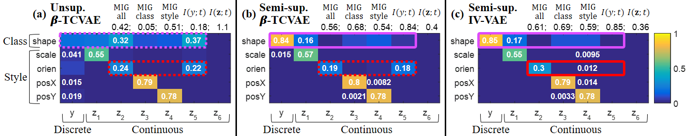
Figure 2: Examples of disentanglement scores (top right) and empirical mutual information (bottom) between the ground truth generative factors of dSprites (y-axis) and inferred features (x-axis). (a) Unsupervised $\beta$-TCVAE ($\beta_{z}=4$). (b) Semi-supervised $\beta$-TCVAE ($\beta_{z}=4$). (c) Semi-supervised IV-VAE (ours; $\beta_{z}=4$ and $\lambda=4$). The three networks were initiated from the same random seed. The dotted-line boxes indicate undesirable results, while the solid-line boxes indicate improved results. The SSL with weak class supervision helps $y$ better capture discrete class factors (pink boxes). The vector independence objective helps $y$ and z store different information, leading to better disentanglement (red boxes).

Figure 3: Comparison on dSprites under the unsupervised (black) and semi-supervised setups with 0.25% (red) and 2% (blue) labeled data. For each network setting, the mean and std scores from 7 random seeds are shown. The x-axis shows $\beta$-VAE, $\beta$-TCVAE, and our IV-VAE trained with the same weight of ELBO KL or TC term ($\beta=\beta_{z}=4$). The $\lambda$ weight for vector independence varies as 1, 4, and 8. Unsupervised learning causes the class factor to be stored in the continuous z instead of the discrete $y$ (i.e., high $I(\textbf{z};t)$ and low $I(y;t)$). Furthermore, the class information is captured in multiple variables, causing lower $\text{MIG}_{\text{class}}$ than $\text{MIG}_{\text{style}}$. Introducing weak supervision with a few labeled data effectively relieves this issue (i.e., low $I(\textbf{z};t)$ and high $I(y;t)$). Our vector independence objective allows $y$ and z to capture different information, improving most of the scores. Keep in mind that the baselines were also trained under the same SSL setup using z and the discrete $y$.

The entangled results for the case where one variable captures both style and class factors (e.g., $z_{2}$ in Figure 2(a)) can obtain fairly good $\text{MIG}_{\text{all}}$ scores. To alleviate this issue, we separately computed the MIG for the class and style factors as $\text{MIG}_{\text{class}}=\text{MIG}_{t}$ (i.e., the MIG of the first row in Figure 2) and $\text{MIG}_{\text{style}}=\frac{1}{|S|}\sum_{m\in S}\text{MIG}_{m}$ (i.e., the mean MIG averaged from the second to last rows), where $t$ denotes ground truth class labels and $S$ is the set of style factors. For the cases without known generative factors but with available labels, $t$, we also computed the MI that assesses how much $y$ represents the class information and z does not as $I(y;t)$ and $I(\textbf{z};t)=\sum_{j}I(z_{j};t)$, respectively.

5 Experimental Results

All results presented in this section were obtained using test data. See our supplementary material for additional results.

5.1 Results on dSprites

5.1.1 Effect of SSL and Vector Independence

Figure 2 depicts the benefit of SSL and vector independence. Using purely unsupervised learning failed to capture the class factor with discrete variable $y$, but employing SSL with 2% class labels easily resolved this issue. Encouraging vector independence helped z better capture the style factors by forcing $y$ and z to store different information.

Figure 3 shows the results on dSprites obtained under various SSL setups. The unsupervised setup yielded good vanilla $\text{MIG}_{\text{all}}$ scores, which were similar to those of the 2%-labeled setup. However, the unsupervised setup caused the continuous vector z to mostly captured the class information and the discrete $y$ to fail to store it. This is evidenced by higher $I(\textbf{z};t)$ and lower $I(y;t)$ than those of the SSL setups. Furthermore, as indicated by lower $\text{MIG}_{\text{class}}$ scores, more than two variables undesirably captured the class factor under the unsupervised setup.

Injecting weak class supervision to the training process simply yet effectively alleviated this difficulty, as shown in the decreased $I(\textbf{z};t)$ and increased $I(y;t)$ in Figure 3. In addition, our IV-VAEs with proper $\lambda$ weights outperformed $\beta$-VAEs and $\beta$-TCVAEs for most scores. In particular, the score improvements with the 0.25% labels were larger than those with the 2% labels, indicating the benefit of vector independence under a few class labels. In terms of the ELBO, our IV-VAEs did not outperform $\beta$-TCVAEs but showed less trade-off between density modeling and disentanglement than $\beta$-VAE (i.e., higher ELBO and MIG scores).

Figure 4: Relationship between the vector independence objective and the evaluation metrics. The x-axis shows vector independence KL $\mathcal{L}^{y,z}_{VecIdp}=\textrm{D}_{\textrm{KL}}\big{(}q_{\phi}(y,\textbf{z})||q_{\phi}(y)q_{\phi}(\textbf{z})\big{)}$, where lower KL values indicate stronger independence. The y-axis shows (a) ELBO, (b) $\text{MIG}_{\text{all}}$, (c) $\text{MIG}_{\text{class}}$, (d) $\text{MIG}_{\text{style}}$, (e) classification error, (f) $I(y;t)$, and (g)$I(\textbf{z};t)$ obtained under the SSL setups with 0.25% and 2% labeled data (denoted by SSL L0.25% and SSL L2%, respectively). Lower is better for (e) and (g), and higher is better for the other metrics. In Figure 4-1 (left), each circle shows the median score of seven networks initiated from different random seeds. As shown in the legend, different colors indicate different $\beta_{z}$ values for controlling the effect of TC in training, and bigger circles indicate bigger $\lambda$ values for causing stronger vector independence. In Figure 4-2 (right), the different $\beta_{z}$ settings are further merged to analyze the overall tendency, and each circle shows the median score of 21 networks (i.e., 7 random seeds $\times$ 3 $\beta_{z}$ settings). Given each setting, the best performing network is indicated with text. As shown in Figure 4-1, given the value of $\beta_{z}$, IV-VAEs often outperform $\beta$-TCVAEs. As shown in Figure 4-2, IV-VAEs with the $\lambda$ of 1 for the 0.25% SSL setup and those with the $\lambda$ of 4 for the 2% SSL setup generally work well.

5.1.2 Relationships between Vector Independence and Evaluation Metrics

Figure 4 shows the relationships between the vector independence objective and evaluation metrics. In Figure 4-1 (left), we depicted scatter plots, where each circle represents the median score of seven networks trained with the same loss weights but initiated from different random seeds. In Figure 4-2 (right), the different $\beta_{z}$ values were further integrated to analyze the general result trends. Notice that in the figures, a larger $\lambda$ led to a smaller KL of vector independence, i.e., a stronger independence between $y$ and z. The analyses are summarized below. See Section S6 for the additional analyses with extended baselines.

• ELBO in Figure 4-1(a). The ELBO values of IV-VAEs were similar to those of $\beta$-TCVAEs for lower $\lambda$ values of 0.5 and 1. Increasing $\lambda$ caused slightly decreased ELBO values, because the models focused more on learning disentangled features than maximizing the reconstruction term. Nevertheless, under higher $\beta_{z}$ values of 4 and 8, IV-VAEs yielded better ELBO than $\beta$-VAEs because we did not penalize the latent-data MI term, which led to an eased trade-off between reconstruction and disentanglement.

• $\text{MIG}_{\text{all}}$, $\text{MIG}_{\text{class}}$, and $\text{MIG}_{\text{style}}$ in Figure 4-1(b), (c), and (d). For most of the $\beta_{z}$ setups, IV-VAEs with the $\lambda$ values of 0.5, 1, or 4 achieved better MIG scores than $\beta$-TCVAEs, showing that reducing the vector independence objective along with the TC helps disentanglement. Higher $\beta_{z}$ that heavily penalized the TC often led to higher MIG scores (i.e., the blue and green lines showed better scores than the red lines). The optimal $\lambda$ yielding the highest MIG differed depending on the value of $\beta_{z}$, but the $\lambda$ of 0.5, 1, and 4 generally worked well.

• Classification error and I(y; t) in Figure 4-1(e) and (f). Given the value of $\beta_{z}$, the lowest classification error and highest $I(y;t)$ score were often obtained with IV-VAE, in comparison to $\beta$-TCVAE. This result implies that vector independence encourages $y$ to better capture the class factor. In the SSL setup with 0.25% labels, excessively increasing $\lambda$ values harmed the classification performance.

• I(z; t) in Figure 4-1(g). IV-VAEs often achieved lower $I(\textbf{z};t)$ than that of $\beta$-TCVAEs. This result implies that vector independence prevents z from storing the class factor by enforcing z and $y$ to represent different information, leading to better disentanglement.

• Overall result trends in Figure 4-2. Our IV-VAEs outperformed $\beta$-TCVAEs for most scores, demonstrating the benefit of vector independence. In general, the $\lambda$ of 1 for the 0.25% setup and the $\lambda$ of 4 for the 2% setup worked well.

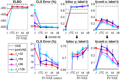
Figure 5: Comparison on Fashion-MNIST with 2% labeled data. For each network setting, the mean and std scores from 10 random seeds are shown. The horizontal lines indicate the mean performance of vanilla VAE and jointVAE. The x-axis shows $\beta$-VAE, $\beta$-TCVAE, and our IV-VAEs. Our IV-VAEs outperform the baselines for most scores, demonstrating the benefit of vector independence. Keep in mind that the baselines were also trained under the same SSL setup using z and the discrete $y$.

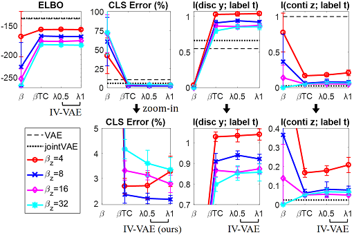
Figure 6: Comparison on MNIST with 2% labeled data. The settings and results are similar to those of Figure 5.

5.2 Results on Fashion-MNIST and MNIST

Figure 5 shows the results on Fashion-MNIST with 2% labeled data. Because of the absence of ground truth style factors, we only measured the MI between the latent variables and class labels. For most values of $\beta_{z}$, promoting vector independence with greater $\lambda$ allowed $y$ and z to capture different factors, causing more class information to be stored in $y$. Our IV-VAEs achieved better classification errors and $I(y;t)$ as well as lower $I(\textbf{z};t)$ than all the baselines, indicating improved disentanglement. Figure 6 shows the results on MNIST with 2% labeled data. We also observed the benefit of our vector independence under most of the $\beta$ weight settings.

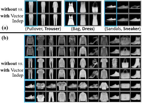
Figure 7: Qualitative results on Fashion-MNIST. (a) Corrected classification. Given an input (left), inferred class probabilities (middle) or one-hot labels (right) from the class encoding $y$ are used for reconstruction. Below each example, inferred labels without and with the vector independence loss are indicated. (b) Style-conditional generation. The style vector z is extracted from an input (leftmost), and the $y$ is set as desired item labels (right). Without promoting vector independence, the network often fails to generate Trouser (the 2nd column in the generation results), Sneaker (the 8th), and Bag (the 9th) classes. Encouraging vector independence forces $y$ to better capture class information in (a) and suitably separates styles from clothing classes in (b).

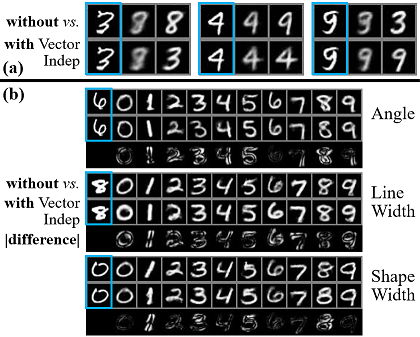
Figure 8: Qualitative results on MNIST. The analysis is similar to that of Figure 7. (a) Corrected classification. (b) Style-conditional generation. In (b), the absolute differences of pixel values are also shown. Encouraging vector independence better exhibits the digit styles (e.g., writing angle, line width, and shape width) by helping z effectively capture style information.

Figures 7 and 8 depict the qualitative results of the two networks trained without and with the vector independence objective. The networks were obtained from the same random seed and loss weights except the $\lambda$ weight. See Section S7 and S8 for additional examples.

To visually show the corrected class labels by encouraging vector independence, Figures 7(a) and 8(a) depict reconstruction examples with estimated class information, i.e., inferred class probabilities or one-hot labels via the argmax operation. The results obtained from the class probabilities were often blurry, indicating that the inputs were confusing to be classified. Employing vector independence often corrects the classification results by enforcing $y$ to better store the class factor.

Figures 7(b) and 8(b) depict the generation examples given input styles. We extracted z from the input and set $y$ as each of the one-hot class labels. Enhancing vector independence better displays the fashion and digit styles by helping z effectively capture style information.

6 Conclusion

We have proposed an approach for semi-supervised disentanglement learning with a variational autoencoder. In our method, two latent vectors separately capture class and style factors. To boost disentanglement, we have proposed the vector independence objective that enforces the vectors to be statistically independent. We have revealed that, along with the total correlation term, our vector independence term is another source of disentanglement in the evidence lower bound. Furthermore, the difficulty in the learning of discrete factors can be reduced by exploiting a small number of class labels. The experiments on the dSprites, Fashion-MNIST, and MNIST datasets have confirmed the effectiveness of our method for image classification and generation.

Contents

1. Variational Bound with Two Latent Vectors

2. Our ELBO Decomposition

3. Relationships between Vector Independence and TC

4. Data and Experimental Settings

5. Baseline Methods

6. In-depth Analysis of Relationships between Vector Independence and Evaluation Metrics

7. Additional Results on Fashion-MNIST

8. Additional Results on MNIST

List of Figures

1. (Derivation) Our decomposition of the KL term in the variational bound with two latent vectors

2. (Derivation) Relationship between the vector independence objective and the separate TC

3. Network architecture

4. Comparison of the collective TC and the separate TC

5. Corrected classification examples on Fashion-MNIST

6. Style-controlled generation on Fashion-MNIST

7. Style-controlled generation on Fashion-MNIST: continued from Figure S6

8. Latent traversal examples on Fashion-MNIST

9. Latent traversal examples on Fashion-MNIST: continued from Figure S8

10. Corrected classification examples on MNIST

11. Style-controlled generation on MNIST

12. Latent traversal examples on MNIST

S1 Variational Bound with Two Latent Vectors

Suppose that the generation process of the data involves two latent vectors, y and z, with a joint prior, $p(\textbf{y},\textbf{z})$. By introducing an approximate posterior, $q_{\phi}(\textbf{y},\textbf{z}|\textbf{x})$, and a likelihood, $p_{\theta}(\textbf{x}|\textbf{y},\textbf{z})$, the ELBO for a single data sample becomes

$$\begin{split}\log p_{\theta}(\textbf{x})&=\log\iint_{\textbf{y},\textbf{z}}p_{\theta}(\textbf{x},\textbf{y},\textbf{z})\,d\textbf{y}d\textbf{z}=\log\iint_{\textbf{y},\textbf{z}}\frac{q_{\phi}(\textbf{y},\textbf{z}|\textbf{x})}{q_{\phi}(\textbf{y},\textbf{z}|\textbf{x})}p_{\theta}(\textbf{x},\textbf{y},\textbf{z})\,d\textbf{y}d\textbf{z}=\log\Big{(}\mathbb{E}_{q_{\phi}(\textbf{y},\textbf{z}|\textbf{x})}\Big{[}\frac{p_{\theta}(\textbf{x},\textbf{y},\textbf{z})}{q_{\phi}(\textbf{y},\textbf{z}|\textbf{x})}\Big{]}\Big{)}\\ &\geq\mathbb{E}_{q_{\phi}(\textbf{y},\textbf{z}|\textbf{x})}\Big{[}\log\frac{p_{\theta}(\textbf{x},\textbf{y},\textbf{z})}{q_{\phi}(\textbf{y},\textbf{z}|\textbf{x})}\Big{]}\qquad\because\mathrm{Jensen^{\prime}s\ inequality}\\ &=\mathbb{E}_{q_{\phi}(\textbf{y},\textbf{z}|\textbf{x})}\Big{[}\log\frac{p_{\theta}(\textbf{x}|\textbf{y},\textbf{z})p(\textbf{y},\textbf{z})}{q_{\phi}(\textbf{y},\textbf{z}|\textbf{x})}\Big{]}=\mathbb{E}_{q_{\phi}(\textbf{y},\textbf{z}|\textbf{x})}\Big{[}\log p_{\theta}(\textbf{x}|\textbf{y},\textbf{z})\Big{]}-\textrm{D}_{\textrm{KL}}\big{(}q_{\phi}(\textbf{y},\textbf{z}|\textbf{x})||p(\textbf{y},\textbf{z})\big{)}.\end{split}$$ (22)

S2 Our ELBO Decomposition

Figure S1 verifies our decomposition of the KL term, $\mathbb{E}_{q(\textbf{x})}\big{[}\textrm{D}_{\textrm{KL}}\big{(}q_{\phi}(\textbf{y},\textbf{z}|\textbf{x})||p(\textbf{y},\textbf{z})\big{)}\big{]}$, in the ELBO on $\mathbb{E}_{q(\textbf{x})}\big{[}\log p_{\theta}(\textbf{x})\big{]}$.

S3 Relationships between Vector Independence and TC

Figure S2 verifies the following relationship: perfect vector independence ensures that the collective TC becomes the sum of the two separate TCs (i.e., $\mathcal{L}^{y,z}_{VecIdp}=0\;\Rightarrow\;\mathcal{L}^{y,z}_{TC}=\mathcal{L}^{y}_{TC}+\mathcal{L}^{z}_{TC}$).

Moreover, in this document, we provide the experimental results regarding the relationship described in (14) of the main paper: $\mathcal{L}^{y,z}_{TC}=0\;\Rightarrow\;\mathcal{L}^{y}_{TC}=\mathcal{L}^{z}_{TC}=\mathcal{L}^{y,z}_{VecIdp}=0$. We show that (i) a perfectly penalized collective TC (i.e., $\mathcal{L}^{y,z}_{TC}=0$) rarely occurs because of the existence of other loss terms (e.g., a reconstruction term) and (ii) encouraging vector independence under penalizing either the separate TC $\mathcal{L}^{z}_{TC}$ or the collective TC $\mathcal{L}^{y,z}_{TC}$ can improve disentanglement performance. See Section S5 for the experimental settings and Section S6 for the results.

Figure S1: Our decomposition of the KL term in the variational bound with two latent vectors. The terms for vector independence (highlighted in red) and variable independence (in green) are depicted.

Figure S2: Relationship between the vector independence objective and the separate TC: perfect vector independence ensures that the collective TC becomes the sum of the two separate TCs.

S4 Data and Experimental Settings

We used the dSprites (Matthey et al., 2017), MNIST (LeCun et al., 2010), and Fashion-MNIST (Xiao et al., 2017) datasets. For semi-supervised learning, the labeled data were selected to be distributed evenly across classes. The size of labeled set $L$ was either 2% or 0.25% of the entire training data, which we used for unlabeled set $U$. The classification loss weight, $\alpha=\rho\frac{N_{L}+N_{U}}{N_{L}}$, was set as $\alpha=51$ for the 2% and 0.25%-labeled dSprites setups. Here, for the 0.25% setup, we failed to apply scaling constant $\rho=1$ (which caused an extremely large $\alpha$), and we instead used $\alpha=51$ as applied in the 2% setup. We used $\alpha=5.1$ (i.e., $\rho=0.1$) for the 2%-labeled MNIST. We used $\alpha=40.8$ (i.e., $\rho=0.8$) for the 2%-labeled Fashion-MNIST.

Figure S3 shows the network architectures used in our experiments, which are identical to the convolutional architectures used in (Dupont, 2018; Jeong & Song, 2019). The priors were set as $p(\textbf{z})=N(\textbf{0},\textbf{I})$ and $p(y)=Cat(\textbf{\textpi})$, where denotes evenly distributed class probabilities. We employed the Gumbel-Softmax distribution (Jang et al., 2017; Maddison et al., 2017) for reparametrizing categorical $y$. We will release our experimental codes on GitHub.

Figure S3: Network architecture for 64×64 (left) and 32×32 (right) images. The yellow and blue boxes indicate the layers of encoder $\phi$ and decoder $\theta$, respectively. Each convolutional (C) or up-convolutional (uC) layer is identified by the size and number of filters. The stride size is 2 for the C and uC layers. Each fully-connected (Fc) layer is identified by the number of output neurons. The concatenation is denoted by “concat.” Each layer is followed by ReLU nonlinearity except that the last encoding layer and output layer are followed by linear and sigmoid activations, respectively. The dashed lines indicate the sampling operation for distributions $q_{\phi}(\textbf{z}|\textbf{x})=N(\textbf{\textmu},\textbf{\textsigma}^{2}\textbf{I})$ and $q_{\phi}(y|\textbf{x})=Cat(\textbf{\textpsi})$.

S4.1 dSprites: 3-class Shape Classification

The dSprites dataset contains 2D-shape binary images with a size of 64$\times$64, which were synthetically generated with five independent factors: shape (3 classes; heart, oval, and square), position X (32 values), position Y (32), scale (6), and rotation (40). We divided the 737,280 images into training, validation, and test sets in a ratio of 10:1:1. We tested two cases with the 2% and 0.25% labels available in the training data.

One 6-dimensional isotropic Gaussian vector was used for $q_{\phi}(\textbf{z}|\textbf{x})$, and one categorical variable representing 3 classes was used for $q_{\phi}(y|\textbf{x})$. The Gumbel-Softmax temperature parameter was set as 0.75. The Adam optimizer was used with an initial learning rate of 0.001 and a minibatch size of 2048. Every batch contained 1024 labeled samples. We trained networks for 100 epochs and reported the results measured at the epoch of the best validation loss. We tested 7 different random weeds for network weight initialization.

S4.2 MNIST: 10-class Digit Classification

The MNIST dataset contains 0–9 handwritten digit images with a size of 28$\times$28. We divided the original training set into 50,000 training and 10,000 validation images while maintaining the test set of 10,000 images. The images were normalized to have [0, 1] continuous values and resized to 32$\times$32 by following (Dupont, 2018). We tested the case with the 2% labels available in the training data.

One 10-dimensional isotropic Gaussian vector was used for $q_{\phi}(\textbf{z}|\textbf{x})$, and one categorical variable representing 10 classes was used for $q_{\phi}(y|\textbf{x})$. The Gumbel-Softmax temperature parameter was set as 0.67. The Adam optimizer was used with an initial learning rate of 0.001 and a minibatch size of 512. Every batch contained 256 labeled samples. We trained networks for 200 epochs and reported the results measured at the epoch of the best validation loss. We tested 10 different random seeds for network weight initialization.

S4.3 Fashion-MNIST: 10-class Fashion Item Classification

The Fashion-MNIST dataset (Xiao et al., 2017) contains grayscale images with a size of 28$\times$28 and 10 fashion categories (e.g., t-shirt, trouser, sandal, and bag). The experimental settings were the same as those used in the MNIST dataset, except that the Gumbel-Softmax temperature parameter was set as 0.75.

S5 Baseline Methods

We assumed that discrete random variable $y\in{\rm I\!R}$ and continuous random vector $\textbf{z}\in{\rm I\!R}^{J}$ were involved in the data generation process. Under this scenario, we compared our IV-VAE with the vanilla VAE (Kingma & Welling, 2014), $\beta$-VAE (Higgins et al., 2017), $\beta$-TCVAE (Chen et al., 2018), and JointVAE (Dupont, 2018). For fair comparison, we applied the following settings that were used in our method to the baselines.

• We utilized the same dimensional latent units and network architectures. For the VAE, $\beta$-VAE, and $\beta$-TCVAE, we augmented the original continuous vector, z, in their objectives with discrete variable $y$. The jointVAE was originally designed to incorporate both of the continuous z and discrete $y$.

• We assumed the conditional independence of $q_{\phi}(y,\textbf{z}|\textbf{x})=q_{\phi}(y|\textbf{x})q_{\phi}(\textbf{z}|\textbf{x})$ by following (Dupont, 2018).

• We modified their original unsupervised setups to use weak classification supervision for semi-supervised learning (SSL). Concretely, as applied in our method, their objectives for labeled set $L$ and unlabeled set $U$ became

  $\mathcal{J}^{L}(\phi,\theta)=\mathcal{J}_{recon}^{L}(\phi,\theta)+\mathcal{J}_{cls}(\phi)-\mathcal{J}^{Both}(\phi)$   and   $\mathcal{J}^{U}(\phi,\theta)=\mathcal{J}_{recon}^{U}(\phi,\theta)-\mathcal{J}^{Both}(\phi)$.

  The reconstruction and classification terms were also identical to those of our method, as shown below. For the reconstruction terms, true label $t$ for $L$ and inferred feature $y$ for $U$ were used to enable the decoder to better recognize one-hot class vectors.

  $\mathcal{J}_{recon}^{L}(\phi,\theta)=\mathbb{E}_{q^{L}(\textbf{x},t)}\Big{[}\mathbb{E}_{q_{\phi}(\textbf{z}|\textbf{x})}\big{[}\log p_{\theta}(\textbf{x}|t,\textbf{z})\big{]}\Big{]}$   and   $\mathcal{J}_{recon}^{U}(\phi,\theta)=\mathbb{E}_{q^{U}(\textbf{x})}\Big{[}\mathbb{E}_{q_{\phi}(y,\textbf{z}|\textbf{x})}\big{[}\log p_{\theta}(\textbf{x}|y,\textbf{z})\big{]}\Big{]}$

  $\mathcal{J}_{cls}(\phi)=\alpha\,\mathbb{E}_{q^{L}(\textbf{x},t)}\Big{[}\mathbb{I}(y=t)\log q_{\phi}(y|\textbf{x})\Big{]}$

The methods differ in the definition of $\mathcal{J}^{Both}(\phi)$ to learn disentangled features and regularize the encoder, as shown below. For notational brevity, we omit the dependence of objectives $\mathcal{J}$ and $\mathcal{L}$ on their parameters $\phi$. The terms related to independence of latent units are indicated by colors (i.e., ${\color[rgb]{0,1,0}\mathcal{L}^{z}_{TC}}$, ${\color[rgb]{0,0,1}\mathcal{L}^{y,z}_{TC}}$, and ${\color[rgb]{1,0,0.87}\mathcal{L}^{y,z}_{VecIdp}}$). Note that we did not penalize the latent-data MI terms by setting $\delta_{y}=\delta_{z}=\delta=0$ in order to help $y$ and z capture the information about x.

• VAE: the case with $\beta=1$ in the below term of $\beta$-VAE

• $\beta$-VAE: $\mathcal{J}^{Both}=\beta\,\mathbb{E}_{q(\textbf{x})}\Big{[}\textrm{D}_{\textrm{KL}}\big{(}q_{\phi}(y,\textbf{z}|\textbf{x})||p(y,\textbf{z})\big{)}\Big{]}=\beta\,\mathbb{E}_{q(\textbf{x})}\Big{[}\textrm{D}_{\textrm{KL}}\big{(}q_{\phi}(y|\textbf{x})||p(y)\big{)}+\textrm{D}_{\textrm{KL}}\big{(}q_{\phi}(\textbf{z}|\textbf{x})||p(\textbf{z})\big{)}\Big{]}$

• $\beta$-TCVAE-1: $\mathcal{J}^{Both}=\Big{(}\delta_{y}\,I_{q_{\phi}}(y;\textbf{x})+\gamma_{y}\,\mathcal{L}^{y}_{Reg}\Big{)}+\Big{(}\delta_{z}\,I_{q_{\phi}}(\textbf{z};\textbf{x})+\beta_{z}\,{\color[rgb]{0,1,0}\mathcal{L}^{z}_{TC}}+\gamma_{z}\,\mathcal{L}^{z}_{Reg}\Big{)}$

• $\beta$-TCVAE-2: $\mathcal{J}^{Both}=\delta\,I_{q_{\phi}}(y,\textbf{z};\textbf{x})+\beta\,{\color[rgb]{0,0,1}\mathcal{L}^{y,z}_{TC}}+\gamma_{y}\,\mathcal{L}^{y}_{Reg}+\gamma_{z}\,\mathcal{L}^{z}_{Reg}$

• JointVAE: $\mathcal{J}^{Both}=\beta\,\mathbb{E}_{q(\textbf{x})}\Big{[}\left|\textrm{D}_{\textrm{KL}}\big{(}q_{\phi}(y|\textbf{x})||p(y)\big{)}-C_{y}\right|\Big{]}+\beta\,\mathbb{E}_{q(\textbf{x})}\Big{[}\left|\textrm{D}_{\textrm{KL}}\big{(}q_{\phi}(\textbf{z}|\textbf{x})||p(\textbf{z})\big{)}-C_{z}\right|\Big{]}$

• IV-VAE-1 (ours): $\mathcal{J}^{Both}=\delta\,I_{q_{\phi}}(y,\textbf{z};\textbf{x})+\lambda\,{\color[rgb]{1,0,0.87}\mathcal{L}^{y,z}_{VecIdp}}+\gamma_{y}\,\mathcal{L}^{y}_{Reg}+\beta_{z}\,{\color[rgb]{0,1,0}\mathcal{L}^{z}_{TC}}+\gamma_{z}\,\mathcal{L}^{z}_{Reg}$

• IV-VAE-2 (ours): $\mathcal{J}^{Both}=\delta\,I_{q_{\phi}}(y,\textbf{z};\textbf{x})+\lambda\,{\color[rgb]{1,0,0.87}\mathcal{L}^{y,z}_{VecIdp}}+\gamma_{y}\,\mathcal{L}^{y}_{Reg}+\beta\,{\color[rgb]{0,0,1}\mathcal{L}^{y,z}_{TC}}+\gamma_{z}\,\mathcal{L}^{z}_{Reg}$

where $\mathcal{L}^{z}_{TC}=\textrm{D}_{\textrm{KL}}\big{(}q_{\phi}(\textbf{z})||\prod\nolimits_{j}q_{\phi}(z_{j})\big{)}$ is the separate TC on z, $\mathcal{L}^{y,z}_{TC}=\textrm{D}_{\textrm{KL}}\big{(}q_{\phi}(y,\textbf{z})||q_{\phi}(y)\prod\nolimits_{j}q_{\phi}(z_{j})\big{)}$ is the collective TC that simultaneously considers $y$ and the variables in z, $\mathcal{L}^{y,z}_{VecIdp}=\textrm{D}_{\textrm{KL}}\big{(}q_{\phi}(y,\textbf{z})||q_{\phi}(y)q_{\phi}(\textbf{z})\big{)}$ is the vector independence term between $y$ and z, and $\mathcal{L}^{y}_{Reg}=\textrm{D}_{\textrm{KL}}\big{(}q_{\phi}(y)||p(y)\big{)}$ and $\mathcal{L}^{z}_{Reg}=\sum\nolimits_{j}\textrm{D}_{\textrm{KL}}\big{(}q_{\phi}(z_{j})||p(z_{j})\big{)}$ are the dimension-wise regularization terms.

The $\mathcal{J}^{Both}$ term of $\beta$-TCVAE-1 is obtained by applying the KL decomposition of (4) in the main paper separately to $\mathbb{E}_{q(\textbf{x})}\big{[}\textrm{D}_{\textrm{KL}}\big{(}q_{\phi}(y|\textbf{x})||p(y)\big{)}\big{]}$ and $\mathbb{E}_{q(\textbf{x})}\big{[}\textrm{D}_{\textrm{KL}}\big{(}q_{\phi}(\textbf{z}|\textbf{x})||p(\textbf{z})\big{)}\big{]}$ in the $\beta$-VAE objective and further assigning individual loss weights to the decomposed terms. Notice that $\mathcal{L}^{y}_{TC}$ does not exist for the single-dimensional variable $y$ (i.e., $\mathcal{L}^{y}_{TC}=\textrm{D}_{\textrm{KL}}\big{(}q_{\phi}(\textbf{y})||\prod\nolimits_{k=1}^{K}q_{\phi}(y_{k})\big{)}$ with $K=1$ is zero). The $\mathcal{J}^{Both}$ term of $\beta$-TCVAE-2 is obtained by applying the KL decomposition of (4) in the main paper to $\mathbb{E}_{q(\textbf{x})}\big{[}\textrm{D}_{\textrm{KL}}\big{(}q_{\phi}(y,\textbf{z}|\textbf{x})||p(y,\textbf{z})\big{)}\big{]}$ in the $\beta$-VAE objective, where the concatenation $[y;\textbf{z}]$ is considered as a single latent vector, and further assigning individual loss weights to the decomposed terms. For fair comparison, we assigned $\gamma_{y}$ and $\gamma_{z}$ separately to $\mathcal{L}^{y}_{Reg}$ and $\mathcal{L}^{z}_{Reg}$ instead of assigning a single $\gamma$ weight to $\mathcal{L}^{y}_{Reg}+\mathcal{L}^{z}_{Reg}$. The $\mathcal{J}^{Both}$ term of JointVAE is identical to the KL term in the original JointVAE objective, where the channel capacity weights $C_{y}$ and $C_{z}$ control the amount of information that $y$ and z can capture. The $\mathcal{J}^{Both}$ term of IV-VAE-1 is identical to (20) in the main paper. The $\mathcal{J}^{Both}$ term of IV-VAE-2 is obtained by changing the TC term in the IV-VAE-1 objective from $\mathcal{L}^{z}_{TC}$ to $\mathcal{L}^{y,z}_{TC}$.

The $\beta$-TCVAE and IV-VAE in the main paper correspond to the $\beta$-TCVAE-1 and IV-VAE-1. In this document, we will present the additional results of $\beta$-TCVAE-2 and IV-VAE-2 along with $\beta$-TCVAE-1 and IV-VAE-1 in Section S6. We will analyze (i) the relationships between the vector independence and evaluation metrics and (2) the effect of penalizing collective TC $\mathcal{L}^{y,z}_{TC}$ or separate TC $\mathcal{L}^{z}_{TC}$ under encouraging vector independence term $\mathcal{L}^{y,z}_{VecIdp}$.

S6 In-depth Analysis of Relationships between Vector Independence and Evaluation Metrics

In the main paper, Figure 4 shows the results of $\beta$-TCVAE-1 and IV-VAE-1 on the dSprites dataset. Here, Figure S4 shows the results of $\beta$-TCVAE-2 and IV-VAE-2 (trained by penalizing the collective TC, $\mathcal{L}^{y,z}_{TC}$) that are merged to those of $\beta$-TCVAE-1 and IV-VAE-1 (trained by penalizing the separate TC, $\mathcal{L}^{z}_{TC}$). The x-axis shows vector independence KL $\mathcal{L}^{y,z}_{VecIdp}=\textrm{D}_{\textrm{KL}}\big{(}q_{\phi}(y,\textbf{z})||q_{\phi}(y)q_{\phi}(\textbf{z})\big{)}$, where lower KL values indicate stronger independence. The y-axis shows (a) ELBO, (b) $\text{MIG}_{\text{all}}$, (c) $\text{MIG}_{\text{class}}$, (d) $\text{MIG}_{\text{style}}$, (e) classification error, (f) $I(y;t)$, and (g)$I(\textbf{z};t)$ obtained under the SSL setups with 0.25% and 2% labeled data (denoted by SSL L0.25% and SSL L2%, respectively). Lower is better for (e) and (g), and higher is better for the other metrics. In Figure S4-1 (left), each circle shows the median score of seven networks initiated from different random seeds. As shown in the legend, different colors indicate different $\beta_{z}$ and $\beta$ values for controlling the effect of TC in training, and bigger circles indicate bigger $\lambda$ values for causing stronger vector independence. In Figure S4-2 (right), the different $\beta_{z}$ or $\beta$ settings are further merged to analyze the overall tendency, and each circle shows the median score of 21 networks (i.e., 7 random seeds $\times$ 3 $\beta_{z}$ or $\beta$ settings).

We compare the effect of the collective TC on disentanglement learning with that of the separate TC. We also show the benefit of encouraging vector independence under penalizing not only the separate TC but also the collective TC. The observations are summarized below.

• In Figure S4-1, given a larger value of $\beta=\beta_{z}$, penalizing the collective TC for $\beta$-TCVAE-2 and IV-VAE-2 yielded stronger vector independence than penalizing the separate TC for $\beta$-TCVAE-1 and IV-VAE-1, e.g., the results for $\beta=8$ (colored by cyan in Figure S4-1) were placed to the left of those for $\beta_{z}=8$ (by blue), whereas the results for $\beta=1$ (by pink) and those for $\beta_{z}=1$ (by red) were similarly placed on the x-axis,. The cause of this phenomenon is that promoting independence between $y$ and all the variables in z by decreasing the collective TC naturally encourages vector independence between $y$ and z (e.g., independence between $y$, $z_{1}$, and $z_{2}$ ensures independence between $y$ and $\textbf{z}=[z_{1},z_{2}]^{T}$). Nevertheless, increasing $\lambda$ for IV-VAE-2 under each $\beta$ setting often led to better vector independence than $\beta$-TCVAE-2 (i.e., $\lambda=0$). This phenomenon is caused by the imperfect minimization of the collective TC because of the existence of the other loss terms (e.g., the reconstruction term).

• In terms of the disentanglement scores, penalizing the separate TC $\mathcal{L}^{z}_{TC}$ on z was competitive with or sometimes outperformed penalizing the collective TC $\mathcal{L}^{y,z}_{TC}$. For example, under the 0.25% SSL setup in Figure S4-2, the best scores of $\text{MIG}_{\text{all}}$, $\text{MIG}_{\text{class}}$, $\text{MIG}_{\text{style}}$, classification error, $I(y;t)$, and $I(\textbf{z};t)$ obtained using the separate TC (text in orange) were better than those using the collective TC (text in purple). Rather than promoting multiple independences via the collective TC (e.g., $y\perp z_{1}$, $y\perp z_{2}$, and $z_{1}\perp z_{2}$), promoting vector independence between $y$ and the entire z (i.e., $y\perp\textbf{z}$) may guide the encoder better to separate discrete and continuous information. Under this guidance, penalizing the separate TC (e.g., $z_{1}\perp z_{2}$) may help each variable capture each continuous factor.

• In Figure S4-2, IV-VAE-2 networks outperformed or were competitive with $\beta$-TCVAE-2 networks for most scores, demonstrating the benefit of vector independence even under penalizing the collective TC. In particular, the $\lambda$ of 0.5 for the 0.25% SSL setup worked well, as shown in the purple text in Figure S4-2. Under the 2% SSL setup, the best performing IV-VAE-2 networks yielded similar results with those of the best $\beta$-TCVAE-2 networks.

S7 Additional Results on Fashion-MNIST

Figures S5, S6, S7, S8, and S9 depict the qualitative results of the two networks trained on Fashion-MNIST without and with the vector independence objective (i.e., $\beta$-TCVAE-1 and IV-VAE-1). The networks were obtained from the same random seed and loss weights except the $\lambda$ weight: the $\lambda$ of 4 was used for training the IV-VAE-1, while the $\beta_{z}$ of 96, $\gamma_{z}$ of 1, and $\gamma_{y}$ of 2 were commonly used for both networks.

To visually show the corrected class labels by encouraging vector independence, Figure S5 depicts reconstruction examples with estimated class information, i.e., inferred class probabilities or one-hot labels via the argmax operation. The results obtained from the class probabilities were often blurry, indicating that the inputs were confusing to be classified. Employing vector independence often corrects the classification results by enforcing $y$ to better store the class factor. Figures S6 and S7 depict generated fashion images given input clothing styles (e.g., brightness and width). We extracted z from the input and set $y$ as each of the one-hot item labels. Without promoting vector independence, the generation of non-clothing items (e.g., sneaker and bag) frequently failed. Encouraging vector independence better disentangled styles from class information, improving the synthesis controllability. The latent traversals in Figures S8 and S9 show that the two dimensions of z captured the continuous factors corresponding to shapes and brightness.

S8 Additional Results on MNIST

Figures S10, S11, and S12 depict the qualitative results of the two networks trained on MNIST without and with the vector independence objective (i.e., $\beta$-TCVAE-1 and IV-VAE-1). The networks were obtained from the same random seed and loss weights except the $\lambda$ weight: the $\lambda$ of 8 was used for training the IV-VAE-1, while the $\beta_{z}$ of 32, $\gamma_{z}$ of 1, and $\gamma_{y}$ of 2 were commonly used for both networks.

Figure S10 shows corrected classification examples, which are visualized using the reconstruction outputs with estimated class information. Figure S11 depicts generation examples of 0–9 digit images given input styles. Encouraging vector independence better displays the digit styles (e.g., writing angle and line width) by helping z effectively capture style information. In Figure S12, the latent traversals on z show the discovered continuous factors of variation.

Figure S4: Comparison of the collective TC and the separate TC. The $\beta$-TCVAE-2 and IV-VAE-2 were trained by penalizing the collective TC $\mathcal{L}^{y,z}_{TC}$ between $y$ and the variables in z, whereas the $\beta$-TCVAE-1 and IV-VAE-1 were trained by penalizing the separate TC $\mathcal{L}^{z}_{TC}$ on z. Given each setting, the best performing network is indicated with text. As shown in Figure S4-1, given a larger value of $\beta_{z}=\beta$, penalizing the collective TC yields stronger vector independence than penalizing the separate TC. Nevertheless, because of the imperfect optimization of the collective TC, increasing $\lambda$ for IV-VAE-2 under each $\beta$ setting often yields better vector independence than $\beta$-TCVAE-2 (i.e., $\lambda=0$). As shown in Figure S4-2, IV-VAE-2 outperforms or is competitive with $\beta$-TCVAE-2 for most scores, demonstrating the benefit of vector independence even under penalizing the collective TC.

Figure S5: Corrected classification examples on Fashion-MNIST. Given an input (left), inferred class probabilities (middle; denoted by “soft”) or one-hot labels (right; denoted by “hard”) from the class encoding $y$ are used for reconstruction. Below each example, inferred labels without and with the vector independence loss are indicated. Encouraging vector independence forces $y$ to better capture class information, improving the classification performance.

Figure S6: Style-controlled generation on Fashion-MNIST. The style feature z is extracted from an input (leftmost), and the class feature $y$ is set as desired item labels (right). Here, the style inputs correspond to top- and whole-body clothing items, and their class number and name are indicated (e.g., L6. Shirt). The order of generation follows the order of original label numbers. Without promoting vector independence, the network often fails to generate Trouser (the 2nd column in the generation results), Sneaker (the 8th), and Bag (the 9th) classes. Encouraging vector independence forces z to better capture style information by suitably separating styles from clothing classes.

Figure S7: Style-controlled generation on Fashion-MNIST: continued from Figure S6. The style feature z is extracted from an input (leftmost), and the class feature $y$ is set as desired item labels (right). Here, the style inputs correspond to bottom clothing and non-clothing fashion items, and their class number and name are indicated (e.g., L1. Trouser). The order of generation follows the order of original label numbers. Without promoting vector independence, the generation with shoe styles frequently fails, as shown in the results of L5, L7, and L9. Encouraging vector independence forces z to better capture style information by suitably separating styles from clothing classes.

Figure S8: Latent traversal examples on Fashion-MNIST. The class feature $y$ and style feature z are extracted from the given inputs (top-most), and the latent traversal results on a single dimension $z_{j}$ are depicted (bottom; traversal range is from -1 to 1). The models capture the continuous factor related to clothing shapes (e.g., width, sleeve length, heel height, and bag size).

Figure S9: Latent traversal examples on Fashion-MNIST: continued from Figure S8 . The class feature $y$ and style feature z are extracted from the given inputs (top-most), and the latent traversal results on a single dimension $z_{j}$ are depicted (bottom; traversal range is from -1 to 1). The models capture the continuous factor related to brightness.

Figure S10: Corrected classification examples on MNIST. Given an input (left), inferred class probabilities (middle; denoted by “soft”) or one-hot labels (right; denoted by “hard”) from the class encoding $y$ are used for reconstruction. Encouraging vector independence forces $y$ to better capture class information, improving the classification performance.

Figure S11: Style-controlled generation on MNIST. The style feature z is extracted from an input (leftmost), and the class feature $y$ is set as desired digit labels (right). The order of generation follows the order of original label numbers. Encouraging vector independence forces z to better capture digit styles such as (a) writing angle, (b) line width, and (c) shape width.

Figure S12: Latent traversal examples on MNIST. The class feature $y$ and style feature z are extracted from the given inputs (top-most), and the latent traversal results on the three dimensions of z are depicted (bottom; traversal range is from -3 to 3). The continuous factors related to digit styles are stored in z.

References

- Amari et al. (1996) Amari, S.-i., Cichocki, A., and Yang, H. H. A new learning algorithm for blind signal separation. In Proc. NIPS, pp. 757–763, 1996.
- Bengio et al. (2013) Bengio, Y., Courville, A., and Vincent, P. Representation learning: A review and new perspectives. IEEE Trans. Pattern Anal. Mach. Intell., 35(8):1798–1828, 2013.
- Burgess et al. (2017) Burgess, C. P., Higgins, I., Pal, A., Matthey, L., Watters, N., Desjardins, G., and Lerchner, A. Understanding disentangling in beta-vae. In Proc. NIPS Workshop, 2017.
- Chen et al. (2018) Chen, T. Q., Li, X., Grosse, R. B., and Duvenaud, D. K. Isolating sources of disentanglement in variational autoencoders. In Proc. NIPS, pp. 2610–2620, 2018.
- Dupont (2018) Dupont, E. Learning disentangled joint continuous and discrete representations. In Proc. NIPS, pp. 710–720, 2018.
- Esmaeili et al. (2019) Esmaeili, B., Wu, H., Jain, S., Bozkurt, A., Siddharth, N., Paige, B., Brooks, D. H., Dy, J., and van de Meent, J.-W. Structured disentangled representations. In Proc. AISTATS, pp. 2525–2534, 2019.
- Gao et al. (2019) Gao, S., Brekelmans, R., Steeg, G. V., and Galstyan, A. Auto-encoding total correlation explanation. In Proc. AISTATS, pp. 1157–1166, 2019.
- Higgins et al. (2017) Higgins, I., Matthey, L., Pal, A., Burgess, C., Glorot, X., Botvinick, M., Mohamed, S., and Lerchner, A. beta-vae: Learning basic visual concepts with a constrained variational framework. In Proc. ICLR, 2017.
- Hoffman & Johnson (2016) Hoffman, M. D. and Johnson, M. J. Elbo surgery: yet another way to carve up the variational evidence lower bound. In Proc. NIPS Workshop, 2016.
- Jang et al. (2017) Jang, E., Gu, S., and Poole, B. Categorical reparameterization with gumbel-softmax. In Proc. ICLR, 2017.
- Jeong & Song (2019) Jeong, Y. and Song, H. O. Learning discrete and continuous factors of data via alternating disentanglement. In Proc. ICML, pp. 3091–3099, 2019.
- Jutten & Herault (1991) Jutten, C. and Herault, J. Blind separation of sources, part i: An adaptive algorithm based on neuromimetic architecture. Signal Processing, 24(1):1–10, 1991.
- Kim & Mnih (2018) Kim, H. and Mnih, A. Disentangling by factorising. In Proc. ICML, pp. 2649–2658, 2018.
- Kim et al. (2006a) Kim, T., Attias, H. T., Lee, S.-Y., and Lee, T.-W. Blind source separation exploiting higher-order frequency dependencies. IEEE Trans. Audio, Speech, Language Process., 15(1):70–79, 2006a.
- Kim et al. (2006b) Kim, T., Eltoft, T., and Lee, T.-W. Independent vector analysis: An extension of ica to multivariate components. In Proc. Int. Conf. on ICA, pp. 165–172, 2006b.
- Kingma & Welling (2014) Kingma, D. P. and Welling, M. Auto-encoding variational bayes. In Proc. ICLR, 2014.
- Kingma et al. (2014) Kingma, D. P., Mohamed, S., Rezende, D. J., and Welling, M. Semi-supervised learning with deep generative models. In Proc. NIPS, pp. 3581–3589, 2014.
- Kumar et al. (2018) Kumar, A., Sattigeri, P., and Balakrishnan, A. Variational inference of disentangled latent concepts from unlabeled observations. In Proc. ICLR, 2018.
- LeCun et al. (2010) LeCun, Y., Cortes, C., and Burges, C. Mnist handwritten digit database. http://yann.lecun.com/exdb/mnist/, 2010.
- Locatello et al. (2019) Locatello, F., Bauer, S., Lucic, M., Raetsch, G., Gelly, S., Schölkopf, B., and Bachem, O. Challenging common assumptions in the unsupervised learning of disentangled representations. In Proc. ICML, pp. 4114–4124, 2019.
- Maaløe et al. (2016) Maaløe, L., Sønderby, C. K., Sønderby, S. K., and Winther, O. Auxiliary deep generative models. In Proc. ICML, pp. 1445–1453, 2016.
- Maddison et al. (2017) Maddison, C. J., Mnih, A., and Teh, Y. W. The concrete distribution: A continuous relaxation of discrete random variables. In Proc. ICLR, 2017.
- Makhzani et al. (2016) Makhzani, A., Shlens, J., Jaitly, N., Goodfellow, I., and Frey, B. Adversarial autoencoders. In Proc. ICLR Workshop, 2016.
- Matthey et al. (2017) Matthey, L., Higgins, I., Hassabis, D., and Lerchner, A. dsprites: Disentanglement testing sprites dataset. https://github.com/deepmind/dsprites-dataset/, 2017.
- Narayanaswamy et al. (2017) Narayanaswamy, S., Paige, T. B., Van de Meent, J.-W., Desmaison, A., Goodman, N., Kohli, P., Wood, F., and Torr, P. Learning disentangled representations with semi-supervised deep generative models. In Proc. NIPS, pp. 5925–5935, 2017.
- Watanabe (1960) Watanabe, S. Information theoretical analysis of multivariate correlation. IBM Journal of research and development, 4(1):66–82, 1960.
- Xiao et al. (2017) Xiao, H., Rasul, K., and Vollgraf, R. Fashion-mnist: a novel image dataset for benchmarking machine learning algorithms. In arXiv preprint arXiv:1708.07747, 2017.
- Zheng & Sun (2019) Zheng, Z. and Sun, L. Disentangling latent space for vae by label relevant/irrelevant dimensions. In Proc. CVPR, pp. 12192–12201, 2019.