Evaluating Logical Generalization in Graph Neural Networks

Supplemental Materials : Evaluating Logical Generalization in Graph Neural Networks

Abstract

Recent research has highlighted the role of relational inductive biases in building learning agents that can generalize and reason in a compositional manner. However, while relational learning algorithms such as graph neural networks (GNNs) show promise, we do not understand how effectively these approaches can adapt to new tasks. In this work, we study the task of logical generalization using GNNs by designing a benchmark suite grounded in first-order logic. Our benchmark suite, GraphLog, requires that learning algorithms perform rule induction in different synthetic logics, represented as knowledge graphs. GraphLog consists of relation prediction tasks on 57 distinct logical domains. We use GraphLog to evaluate GNNs in three different setups: single-task supervised learning, multi-task pretraining, and continual learning. Unlike previous benchmarks, our approach allows us to precisely control the logical relationship between the different tasks. We find that the ability for models to generalize and adapt is strongly determined by the diversity of the logical rules they encounter during training, and our results highlight new challenges for the design of GNN models. We publicly release the dataset and code used to generate and interact with the dataset at https://www.cs.mcgill.ca/ ksinha4/graphlog/.

1 Introduction

Relational reasoning, or the ability to reason about the relationship between objects entities in the environment, is considered a fundamental aspect of intelligence (Krawczyk et al., 2011; Halford et al., 2010). Relational reasoning is known to play a critical role in cognitive growth of children (Son et al., 2011; Farrington-Flint et al., 2007; Richland et al., 2010). This ability to infer relations between objects/entities/situations, and to compose relations into higher-order relations, is one of the reasons why humans quickly learn how to solve new tasks (Holyoak & Morrison, 2012; Alexander, 2016).

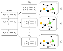
Figure 1: GraphLog setup. We define a large set of rules that are grounded in propositional logic. We partition the rule set into overlapping subsets, which we use to define the unique worlds, $W_{k}$. Finally, within each world $W_{k}$, we generate several knowledge graphs $g_{i}^{k}$ that are governed by the rule set of $W_{k}$.

The perceived importance of relational reasoning for generalization capabilities has fueled the development of several neural network architectures that incorporate relational inductive biases (Battaglia et al., 2016; Santoro et al., 2017; Battaglia et al., 2018). Graph neural networks (GNNs), in particular, have emerged as a dominant computational paradigm within this growing area (Scarselli et al., 2008; Hamilton et al., 2017a; Gilmer et al., 2017; Schlichtkrull et al., 2018; Du et al., 2019). However, despite the growing interest in GNNs and their promise for improving the generalization capabilities of neural networks, we currently lack an understanding of how effectively these models can adapt and generalize across distinct tasks.

In this work, we study the task of logical generalization, in the context of relational reasoning using GNNs. In particular, we study how GNNs can induce logical rules and generalize by combining these rules in novel ways after training. We propose a benchmark suite, GraphLog, that is grounded in first-order logic. Figure 1 shows the setup of the benchmark. Given a set of logical rules, we create different logical worlds with overlapping rules. For each world (say $W_{k}$), we sample multiple knowledge graphs (say $g_{i}^{k}$). The learning agent should learn to induce the logical rules for predicting the missing facts in these knowledge graphs. Using our benchmark, we evaluate the generalization capabilities of GNNs in a supervised setting by predicting unseen combinations of known rules within a specific logical world. This task that explicitly requires inductive generalization. We further analyze how various GNN architectures perform in the multi-task and the continual learning scenarios, where they have to learn over a set of logical worlds with different underlying logic. Our setup allows us to control the similarity between the different worlds by controlling the overlap in logical rules between different worlds. This enables us to precisely analyze how task similarity impacts performance in the multi-task setting.

Our analysis provides the following useful insights regarding the logical generalization capabilities of GNNs:

• Two architecture choices for GNNs have a strong positive impact on the generalization performance: 1) incorporating multi-relational edge features using attention, and 2) explicitly modularising the GNN architecture to include a parametric representation function, which learns representations for the relations based on the knowledge graph structure.

• In the multi-task setting, training a model on a more diverse set of logical worlds improves generalization and adaptation performance.

• All the evaluated models exhibit catastrophic forgetting in the continual learning setting. This indicates that the models are prone to fitting to just the current task at hand and not learning representations and compositions that can transfer across tasks—highlighting the challenge of lifelong learning in the context of logical generalization and GNNs.

2 Background and Related Work

Graph Neural Networks. Several graph neural network (GNN) architectures have been proposed to learn the representation for the graph input (Scarselli et al., 2008; Duvenaud et al., 2015; Defferrard et al., 2016; Kipf & Welling, 2016; Gilmer et al., 2017; Veličković et al., 2017; Hamilton et al., 2017b; Schlichtkrull et al., 2018). Previous works have focused on evaluating graph neural networks in terms of their expressive power (Morris et al., 2019; Xu et al., 2018), usefulness of features (Chen et al., 2019), and explaining the predictions from GNNs (Ying et al., 2019). Complementing these works, we evaluate GNN models on the task of logical generalization.

Knowledge graph completion. Many knowledge graph datasets are available for the task of relation prediction (also known as knowledge base completion). Prominent examples include Freebase15K (Bordes et al., 2013), WordNet (Miller, 1995), NELL (Mitchell & Fredkin, 2014), and YAGO (Suchanek et al., 2007; Hoffart et al., 2011; Mahdisoltani et al., 2013). These datasets are derived from real-world knowledge graphs and are useful for empirical evaluation of relation prediction systems. However, these datasets are generally noisy and incomplete, as many facts are not available in the underlying knowledge bases (West et al., 2014; Paulheim, 2017). Moreover, the logical rules underpinning these systems are often opaque and implicit (Guo et al., 2016). All these shortcomings reduce the usefulness of existing knowledge graph datasets for understanding the logical generalization capability of neural networks. Some of these limitations can be overcome by using synthetic datasets, which can provide a high degree of control and flexibility over the data generation process at a low cost. Synthetic datasets are useful for understanding the behavior of different models - especially when the underlying problem can have many factors of variations. We consider using synthetic datasets, as a means and not an end, to understand the logical generalization capability of GNNs.

Our GraphLog benchmark serves as a synthetic complement to the real-world datasets. Instead of sampling from a real-world knowledge base, we create synthetic knowledge graphs that are governed by a known and inspectable set of logical rules. Moreover, the relations in GraphLog are self-contained and do not require any common-sense knowledge, thus making the tasks self-contained.

Procedurally generated datasets for reasoning. In recent years, several procedurally generated benchmarks have been proposed to study the relational reasoning and compositional generalization properties of neural networks. Some recent and prominent examples are listed in Table 1. These datasets aim to provide a controlled testbed for evaluating the compositional reasoning capabilities of neural networks in isolation. Based on these existing works and their insightful observations, we enumerate the four key desiderata that, we believe, such a benchmark should provide:

1. Interpretable Rules: The rules that are used to procedurally generate the dataset should be human interpretable.

2. Diversity: The benchmark datasets should have enough diversity across different tasks, and the compositional rules used to solve different tasks should be distinct, so that adaptation on a novel task is not trivial. The degree of similarity across the tasks should be configurable to enable evaluating the role of diversity in generalization.

3. Compositional generalization: The benchmark should require compositional generalization, i.e., generalization to unseen combinations of rules.

4. Number of tasks: The benchmark should support creating a large number of tasks. This enables a more fine-grained inspection of the generalization capabilities of the model in different setups, e.g., supervised learning, multitask learning, and continual learning.

As shown in Table 1, GraphLog is unique in satisfying all of these desiderata. We highlight that GraphLog is the only dataset specifically designed to test logical generalization capabilities on graph data, whereas previous works have largely focused on the image and text modalities.

Dataset	IR	D	CG	M	S	Me	Mu	CL
CLEVR (Johnson et al., 2017)	✓	✗	✗	Vision	✓	✗	✗	✗
CoGenT (Johnson et al., 2017)	✓	✗	✓	Vision	✓	✗	✗	✗
CLUTRR (Sinha et al., 2019)	✓	✗	✓	Text	✓	✗	✗	✗
SCAN (Lake & Baroni, 2017)	✓	✗	✓	Text	✓	✓	✗	✗
SQoOP (Bahdanau et al., 2018)	✓	✗	✓	Vision	✓	✗	✗	✗
TextWorld (Côté et al., 2018)	✗	✓	✓	Text	✓	✓	✓	✓
GraphLog (Proposed)	✓	✓	✓	Graph	✓	✓	✓	✓

Table 1: Features of related datasets that are: 1) designed to test compositional generalization and reasoning, and 2) procedurally gnerated. We compare the datasets along the following dimensions: Inspectable Rules (IR), Diversity, Compositional Generalization (CG), Modality and if the following training setups are supported: Supervised, Meta-learning, Multitask & Continual learning (CL).

3 GraphLog

3.1 Terminology

A graph $G=(V_{G},E_{G})$ is a collection of a set of nodes $V_{G}$ and a set of edges $E_{G}$ between the nodes. In this work, we assume that each pair of nodes have at most one edge between them. A relational graph is a graph where the edge between two nodes (say $u$ and $v$) is assigned a label, denoted $r$. The labeled edge is denoted as $(u\rightarrow_{r}v)\in E_{G}$. A relation set $R$ is a set of relations $\{r_{1}$, $r_{2}$, … $r_{K}\}$. A rule set $\mathcal{R}$ is a set of rules in first order logic, which we denote in the Datalog format (Evans & Grefenstette, 2017), $[r_{i},r_{j}]\Rightarrow r_{k}$, and which can be expanded as Horn clauses of the form:

$$\exists z\in V_{G}:(u\rightarrow_{r_{i}}z)\land(z\rightarrow_{r_{j}}v)\Rightarrow(u\rightarrow_{r_{k}}v)$$ (1)

where $z$ denotes a variable that can be bound to any entity and $\Rightarrow$ denotes logical implication. The relations $r_{i},r_{j}$ form the body while the relation $r_{k}$ forms the head of the rule. Horn clauses of this form represent a well-defined subset of first-order logic, and they encompass the types of logical rules learned by the vast majority of existing rule induction engines for knowledge graphs (Langley & Simon, 1995).

We use $p_{G}^{u,v}$ to denote a path from node $u$ to $v$ in a graph $G$. We construct graphs according to rules of the form in Equation 1 so that a path between two nodes will always imply a specific relation between these two nodes. In other words, we will always have that

$$\exists r_{i}\in\mathcal{R}\>:\>p_{G}^{u,v}\Rightarrow(u\rightarrow_{r_{i}}v).$$ (2)

Thus, following the path between two nodes, and applying the propositional rules along the edges of the path, we can resolve the relationship between the nodes. Hence, we refer to the paths as resolution paths. The edges of the resolution path are concatenated together to obtain a descriptor. These descriptors are used for quantifying the similarity between different resolution paths, with a higher overlap between the descriptors implying a greater similarity between two resolution paths.

3.2 Problem Setup

We formulate the relational reasoning task as predicting relations between the nodes in a relational graph. Given a query $(G,u,v)$ where $u,v\in V_{G}$, the learner has to predict the relation $r_{?}$ for the edge $u\rightarrow_{r_{?}}v$. Unlike the previous work on knowledge graph completion, we emphasize an inductive problem setup, where the graph $G$ in each query is unique. Rather than reasoning on a single static knowledge graph during training and testing, we consider the setting where the model must learn to generalize to unseen graphs during evaluation.

3.3 Dataset Generation

As discussed in Section 2, we want our proposed benchmark to provide four key desiderata: (i) interpretable rules, (ii) diversity, (iii) compositional generalization and (iv) large number of tasks. We describe how our dataset generation process ensures all four aspects.

Rule generation. We create a set $R$ of $K$ relations and use it to sample a rule set $\mathcal{R}$. We impose two constraints on $\mathcal{R}$: (i) No two rules in $\mathcal{R}$ can have the same body. This ensures consistency between the rules. (ii) Rules cannot have common relations among the head and body. This ensures the absence of cyclic dependencies in rules (Hamilton et al., 2018). Generating the dataset using a consistent and well-defined rule set ensures interpretability in the resulting dataset. The full algorithm for rule generation is given in Appendix (Algorithm 1).

Graph generation. The graph generation process has two steps: In the first step, we recursively sample and use rules in $\mathcal{R}$ to generate a relational graph called the WorldGraph (as shown in Figure 1). This sampling procedure enables us to create a diverse set of WorldGraphs by considering only certain subsets (of $\mathcal{R}$) during sampling. By controlling the extent of overlap between the subsets of $\mathcal{R}$ (in terms of the number of rules that are common across the subsets), we can precisely control the similarity between the different WorldGraphs. The full algorithm for generating the WorldGraph and controlling the similarity between the worlds is given in Appendix (Algorithm 3 and Section A.2).

In the second step, the WorldGraph $G_{W}$ is used to sample a set of graphs $G_{W}^{S}=(g_{1},\cdots g_{N})$ (shown as Step (a) in Figure 2). A graph $g_{i}$ is sampled from $G_{W}$ by sampling a pair of nodes $(u,v)$ from $G_{W}$ and then by sampling a resolution path $p_{G_{W}}^{u,v}$. The edge $u\rightarrow_{r_{i}}v$ between the source and sink node of the path provides the target relation for the learning model to predict. To increase the complexity of the sampled $g_{i}$ graphs (beyond being simple paths), we also add nodes to $g_{i}$ by sampling neighbors of the nodes on $p_{G_{W}}^{u,v}$, such that no other shortest path exists between $u$ and $v$. Algorithm 4 (in the Appendix) details our graph sampling approach.

3.4 Summary of the GraphLog Dataset

We use the data generation process described in Section 3.3 to instantiate a dataset suite with 57 distinct logical worlds and $5000$ graphs per world (Figure 1). The dataset is divided into the sets of training, validation, and testing worlds. The graphs within each world are also split into training, validation, and testing sets. The key statistics of the datasets are given in Table 2. Though we instantiate 57 worlds, the GraphLog code can instantiate an arbitrary number of worlds and has been included in the supplementary material.

3.4.1 Setups supported in GraphLog

GraphLog enables us to investigate the logical relational reasoning performance of models in the following setups:

Number of relations	20
Total number of WorldGraphs	57
Total number of unique rules	76
Training Graphs per WorldGraph	5000
Validation Graphs per WorldGraph	1000
Testing Graphs per WorldGraph	1000
Number of rules per WorldGraph	20
Average number of descriptors	522
Maximum length of resolution path	10
Minimum length of resolution path	2

Table 2: Aggregate statistics of the worlds used in GraphLog. Statistics for each individual world are in the Appendix.

Supervised learning. In the supervised learning setup, a model is trained on the train split of a single logical world and evaluated on the test split of the same world. The total number of rules grows exponentially with the number of relations $K$, making it impossible to train on all possible combinations of the relations. However, we expect that a perfectly systematic model generalizes to unseen combinations of relations by training only on a subset of combinations (i.e., via inductive reasoning).

Multi-task learning. GraphLog provides multiple logical worlds, each with its own training and evaluation splits. In the standard multi-task training, the model is trained on the train split of many worlds ($W_{1},\cdots,W_{M})$ and evaluated on the test split of the same worlds. The complexity of each world and the similarity between the different worlds can be precisely controlled. GraphLog thus enables us to evaluate how model performance varies when the model is trained on similar vs. dissimilar worlds.

GraphLog is also designed to study the effect of pre-training on adaptation. In this setup, the model is first pre-trained on the train split of multiple worlds ($W_{1},\cdots,W_{M}$) and then adapted (fine-tuned) on the train split of the unseen heldout worlds ($W_{M+1},\cdots,W_{N})$. The model is evaluated on the test split of the novel worlds. Similar to the previous setup, GraphLog provides us an opportunity to investigate the effect of similarity in pre-training. This enables GraphLog to mimic in-distribution and out-of-distribution training and testing scenarios, as well as precisely categorize the effect of multi-task pre-training for adaptation performance.

Continual learning. GraphLog provides access to a large number of worlds, enabling us to evaluate the logical generalization capability of the models in the continual learning setup. In this setup, the model is trained on a sequence of worlds. Before training on a new world, the model is evaluated on all the worlds that the model has trained on so far. Given the several challenges involved in continual learning (Thrun & Pratt, 2012; Parisi et al., 2019; De Lange et al., 2019; Sodhani et al., 2019), we do not expect the models to be able to remember the knowledge from all the previous tasks. Nonetheless, given that we are evaluating the models for relational reasoning and that our datasets share relations, we would expect the models to retain some knowledge of how to solve the previous tasks. In this sense, the performance on the previous tasks can also be seen as an indicator of if the models actually learn to solve the relational reasoning tasks or they just fit to the current dataset distribution.

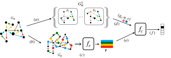
Figure 2: Overview of the training process: (a): Sampling multiple graphs from $G_{W}$. (b): Converting the relational graph into extended graph $\hat{G_{W}}$. Note that edges of different color (denoting different types of relations) are replaced by a node of same type in $\hat{G}_{W}$. (c): Learning representations of the relations ($\mathbf{r}$) using $f_{r}$ with the extended graph as the input. In case of Param models, the relation representations are parameterized via an embedding layer and the extended graph is not created. (d, e): The composition function takes as input the query $g_{i},u,v$ and the relational representation $\mathbf{r}$. (f): The composition function predicts the relation between the nodes $u$ and $v$.

4 Representation and Composition

In this section, we describe the graph neural network (GNN) architectures that we evaluate on the GraphLog benchmark. In order to perform well on the benchmark tasks, a model should learn representations that are useful for solving the tasks in the current world while being general enough to be effectively adapted to the new worlds. To this end, we structure the GNN models we analyze around two key modules:

• Representation module: This module is represented as a function $f_{r}:G_{W}\times R\rightarrow\mathbb{R}^{d}$, which maps logical relations within a particular world $W$ to $d$-dimensional vector representations. Intuitively, this function should learn how to encode the semantics of the various relations within a logical world.

• Composition module: This module is a function $f_{c}:G_{W}\times V_{G_{W}}\times V_{G_{W}}\times\mathbb{R}^{d\times|R|}\rightarrow R$, which learns how to compose the relation representations learned by $f_{r}$ to make predictions about queries over a knowledge graph.

Note that though we break down the process into two steps, in practice, the learner does not have access to the correct representations of relations or to $\mathcal{R}$. The learner has to rely only on the target labels to solve the reasoning task. We hypothesize that this separation of concerns between a representation function and a composition function (Dijkstra, 1982) could provide a useful inductive bias for the model.

4.1 Representation modules

We first describe the different approaches for learning the representation $\mathbf{r}_{i}\in\mathbb{R}^{d}$ for the relations. These representations will be provided as input to the composition function.

Direct parameterization. The simplest approach to define the representation module is to train unique embeddings for each relation $r_{i}$. This approach is predominantly used in the previous work on GNNs (Gilmer et al., 2017; Veličković et al., 2017), and we term this approach as the Param representation module. A major limitation of this approach is that the relation representations are optimized specifically for each logical world, and there is no inductive bias towards learning representations that can generalize.

Learning representations from the graph structure. In order to define a more powerful and expressive representation function, we consider an approach that learns relation representations as a function of the WorldGraph underlying a logical world. To do so, we consider an “extended” form of the WorldGraph, $\hat{G}_{W}$, where introduce new nodes (called edge-nodes) corresponding to each edge in the original WorldGraph $G_{W}$. For an edge $(u\rightarrow_{r}v)\in E_{G}$, the corresponding edge-node $(u-r-v)$ is connected to only those nodes that were incident to it in the original graph (i.e. nodes $u$ and $v$; see Figure 2, Step (b)). This new graph $\hat{G}_{W}$ only has one type of edge and comprises of nodes from both the original graph and from the set of edge-nodes.

We learn the relation representations by training a GNN model on the expanded WorldGraph and by averaging the edge-node embeddings corresponding to each relation type $r_{i}\in R$. (Step (c) in Figure 2). For the GNN model, we consider the Graph Convolutional Network (GCN) (Kipf & Welling, 2016) and the Graph Attention Network (GAT) architectures. Since the nodes do not have any features or attributes, we randomly initialize the embeddings in these GNN message passing layers.

The intuition behind creating the extended-graph is that the representation GNN function can learn the relation embeddings based on the structure of the complete relational graph $G_{W}$. We expect this to provide an inductive bias that can generalize more effectively than the simple Param approach. Finally, note that while the representation function is given access to the WorldGraph to learn representations for relations, the composition module is not able to interface with the WorldGraph in order to make predictions about a query.

4.2 Composition modules

We now describe the GNNs used for the composition modules. These models take as input the query $(g_{i},u,v)$ and the relation embedding $\mathbf{r}_{i}\in\mathbb{R}^{d}$ (Step (d) and (e) in Figure 2).

Relational Graph Convolutional Network (RGCN). Given that the input to the composition module is a relational graph, the RGCN model (Schlichtkrull et al., 2018) is a natural choice for a baseline architecture. In this approach, we iterate a series of message passing operations:

$$\mathbf{h}_{u}^{(t)}=\textrm{ReLU}\left(\sum_{r_{i}\in R}\sum_{v\in\mathcal{N}_{r_{i}}(u)}\mathbf{r}_{i}\times_{1}\mathcal{T}\times_{3}\mathbf{h}_{v}^{(t-1)}\right),$$

where $\mathbf{h}^{(t)}_{u}\in\mathbb{R}^{d}$ denotes the representation for a node $u$ at the $t^{th}$ layer of the model, $\mathcal{T}\in\mathbb{R}^{d_{r}\times d\times d}$ is a learnable tensor, $\mathbf{r}\in\mathbb{R}^{d}$ is the representation for relation $r$, and $\mathcal{N}_{r_{i}}(u)$ denotes the neighbors of node $u$ by relation $r_{i}$. We use $\times_{i}$ to denote multiplication across a particular mode of the tensor. This RGCN model learns a relation-specific propagation matrix, specified by the interaction between the relation embedding $\mathbf{r}_{i}$ and the shared tensor $\mathcal{T}$.

Edge-based Graph Attention Network (Edge-GAT). In addition to the RGCN model—which is considered the defacto standard architecture for applying GNNs to multi-relational data—we also explore an extension of the Graph Attention Network (GAT) model (Veličković et al., 2017) to handle edge types. Many recent works have highlighted the importance of the attention mechanism, especially in the context of relational reasoning (Vaswani et al., 2017; Santoro et al., 2018; Schlag et al., 2019). Motivated by this observation, we investigate an extended version of the GAT, where we incorporate gating via an LSTM (Hochreiter & Schmidhuber, 1997) and where the attention is conditioned on both the incoming message (from the other nodes) and the relation embedding (of the other nodes):

$$\mathbf{m}_{\mathcal{N}(u)} =\sum_{r_{i}\in R}\sum_{v\in\mathcal{N}_{r_{i}}(u)}\alpha\left(\mathbf{h}_{u}^{(t-1)},\mathbf{h}^{(t-1)}_{v},\mathbf{r}\right)$$

$$\mathbf{h}_{u}^{(t)} =\textrm{LSTM}(\mathbf{m}_{\mathcal{N}(u)},\mathbf{h}_{u}^{(t-1)})$$

Following the original GAT model, the attention function $\alpha$ is defined using an dense neural network on the concatenation of the input vectors. We refer to this model as the Edge GAT (E-GAT) model.

Query and node representations. We predict the relation for a given query $(g_{i},u,v)$ by concatenating $\mathbf{h}^{(K)}_{u},\mathbf{h}^{(K)}_{v}$ (the final-layer query node embeddings, assuming a $K$-layer GNN) and applying a two-layer dense neural network (Step (f) in Figure 2). The entire model (i.e., the representation function and the composition function) are trained end-to-end using the softmax cross-entropy loss. Since we have no node features, we randomly initialize all the node embeddings in the GNNs (i.e., $\mathbf{h}_{u}^{(0)}$).

5 Experiments

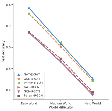
Figure 3: We categorize the datasets in terms of their relative difficulty (see Appendix). We observe that the models using E-GAT as the composition function consistently work well.

We aim to quantify the performance of the different GNN models on the task of logical relation reasoning, in three contexts: (i) Single Task Supervised Learning, (ii) Multi-Task Training and (iii) Continual Learning. Our experiments use the GraphLog benchmark with distinct 57 worlds or knowledge graph datasets (see Section 3) and 6 different different GNN models (see Section 4). In the main paper, we share the key trends and observations that hold across the different combinations of the models and the datasets, along with some representative results. The full set of results is provided in the Appendix. All the models are implemented using PyTorch 1.3.1 (Paszke et al., 2019). The code has been included with the supplemental material.

5.1 Single Task Supervised Learning

In our first setup, we train and evaluate all of the models on all the 57 worlds, one model, and one world pair at a time. This experiment provides several important results. Previous works considered only a handful of datasets when evaluating the different models on the task of relational reasoning. As such, it is possible to design a model that can exploit the biases present in the few datasets that the model is being evaluated over. In our case, we consider over 50 datasets, with different characteristics (Table 2). It is difficult for one model to outperform the other models on all the datasets just by exploiting some dataset-specific bias, thereby making the conclusions more robust.

In Figure 3, we present the results for the different models. We categorize the worlds in three categories of difficulty – easy, moderate and difficult – based on relative test performance of the models on each world. Table 6 (in Appendix) contains the results for the different models on the individual worlds. We observe that the models using E-GAT as the composition functions always outperform their counterparts using the RGCN models. This confirms our hypothesis about the usefulness of combining relational reasoning and attention for improving the performance on relational reasoning tasks. An interesting observation is that the relative ordering among the worlds, in terms of the test accuracy of the different models, is consistent irrespective of the model we use, highlighting the intrinsic difficulty of the different worlds in GraphLog.

5.2 Multi-Task Training

		S	D
$f_{r}$	$f_{c}$	Accuracy	Accuracy
GAT	E-GAT	0.534 $\pm{0.11}$	0.534 $\pm{0.09}$
GAT	RGCN	0.474 $\pm{0.11}$	0.502 $\pm{0.09}$
GCN	E-GAT	0.522 $\pm{0.1}$	0.533 $\pm{0.09}$
GCN	RGCN	0.448 $\pm{0.09}$	0.476 $\pm{0.09}$
Param	E-GAT	0.507 $\pm{0.09}$	0.5 $\pm{0.09}$
Param	RGCN	0.416 $\pm{0.07}$	0.449 $\pm{0.07}$

Table 3: Multitask evaluation performance when trained on different data distributions. We categorize the training distribution on basis of their similarity of rules: Similar (S) containing similar worlds and a mix of similar and dissimilar worlds (D)

We now turn to the setting of multi-task learning where we train the same model on multiple logical worlds.

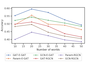
Figure 4: We run multitask experiments over an increasing number of worlds to stretch the capacity of the models. Evaluation performance is reported as the average of test set performance across the worlds that the model has trained on so far. All the models reach their optimal performance at 20 worlds, beyond which their performance starts to degrade.

Basic multi-task training. First, we evaluate a how changing the similarity among the training worlds affects the test performance in the multi-task setup, where a model is trained jointly on eight and tested on three distinct worlds. In Table 3, we observe that considering a mix of similar and dissimilar worlds improves the generalization capabilities of all the models when evaluated on the test split. Another important observation is that just like the supervised learning setup, the GAT-EGAT model consistently performs either as good as or better than other models and the models using EGAT for the composition function perform better than the ones using the RGCN model. Figure 4 shows how the performance of the various models changes when we perform multi-task training on an increasingly large set of worlds. Interestingly, we see that model performance improves as the number of worlds is increased from 10 to 20 but then begins to decline, indicating capacity saturation in the presence of too many diverse worlds.

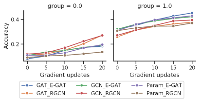
Figure 8: We perform fine-grained analysis of few shot adaptation capabilities in Multitask setting. Group 0.0 and 1.0 corresponds to 0% and 100% similarity respectively.

Multi-task pre-training. In this setup, we pre-train the model on multiple worlds and adapt on a heldout world. We study how the models’ adaption capabilities vary as the similarity between the training and the evaluation distributions changes. Figure 5 considers the case of zero-shot adaptation and adaptation till convergence. As we move along the x-axis, the zero-shot performance (shown with solid colors) decreases in all the setups. This is expected as the similarity between the training and the evaluation distributions also decreases. An interesting trend is that the model’s performance, after adaptation, increases as the similarity between the two distributions decreases. This suggests that training over a diverse set of distributions improves adaptation capability. The results for adaptation with 5, 10, … 30 steps are provided in the Appendix (Figure 8).

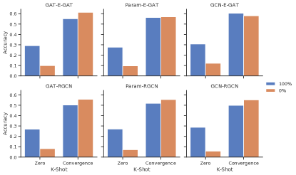
Figure 5: We evaluate the effect of changing the similarity between the training and the evaluation datasets. The colors of the bars depicts how similar the two distributions are while the y-axis shows the mean accuracy of the model on the test split of the evaluation world. We report both the zero-shot adaptation performance and performance after convergence.

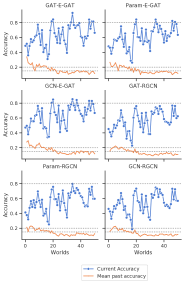
Figure 6: We evaluate the performance of all the models in a continual learning setup. The blue curve shows the accuracy on the current world and the orange curve shows the mean accuracy on all the previously seen worlds. As the model trains on new worlds, its performance on the previously seen worlds degrades rapidly. This is the forgetting effect commonly encountered in continual learning setups.

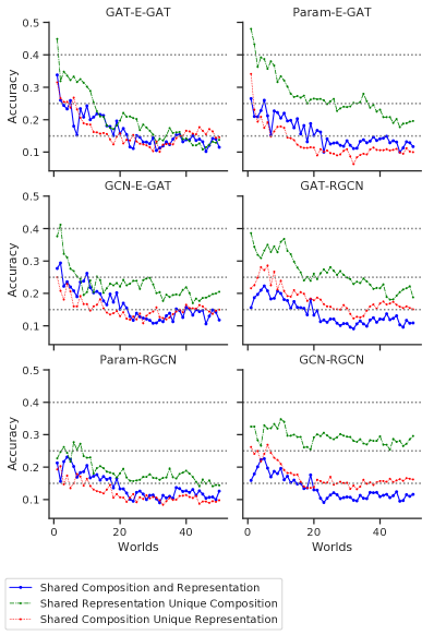
Figure 7: We evaluate the performance in a continual learning setup where we share either the representation function or the composition function or both. We observe that sharing the representation function reduces the effect of catastrophic forgetting as compared to the other setups.

5.3 Continual Learning Setup

In the continual learning setup, we evaluate the knowledge retention capabilities of the GNN models. We train the model on a sequence of overlapping worlds, and after converging on every world, we report the average of model’s performance on all the previous worlds. In Figure 6 we observe that as the model is trained on different worlds, the performance on the previous worlds degrades rapidly. This highlights that the current reasoning models are not suitable for continual learning.

The role of the representation function. We also investigate the model’s performance in a continual learning setup where the model learns only a world-specific representation function or a world-specific composition function, and where the other module is shared across the worlds. In Figure 7, we observe that sharing the representation function reduces the effect of catastrophic forgetting, but sharing the composition function does not have the same effect. This suggests that the representation function learns representations that are useful across the worlds.

6 Discussion & Conclusion

In this work, we propose GraphLog, a benchmark suite for evaluating the logical generalization capabilities of Graph Neural Networks. GraphLog is grounded in first-order logic and provides access to a large number of diverse tasks that require compositional generalization to solve, including single task supervised learning, multi-task learning, and continual learning. Our results highlight the importance of attention mechanisms and modularity to achieve logical generalization, while also highlighting open challenges related to multi-task and continual learning in the context of GNNs. A natural direction for future work is leveraging GraphLog for studies of fast adaptation and meta-learning in the context of logical reasoning (e.g., via gradient-based meta learning), as well as integrating state-of-the-art methods (e.g., regularization techniques) to combat catastrophic forgetting in the context of GNNs.

Appendix A GraphLog

A.1 Extended Terminology

In this section, we extend the terminology introduced in Section 3.1. A set of relations is said to be Invertible if

$$\forall r_{i}\in R,\exists r_{j}\in R\mid\{\forall u,v\in V_{G}:(u\rightarrow_{r_{i}}v)\Rightarrow(v\rightarrow_{r_{j}}u)\}.$$ (3)

i.e. for all relations in $R$, there exists a relation in $R$ such that for all node pairs $(u,v)$ in the graph, if there exists an edge $u\rightarrow_{r_{i}}v$ then there exists another edge $v\rightarrow_{r_{j}}u$. Invertible relations are useful in determining the inverse of a clause, where the directionality of the clause is flipped along with the ordering of the elements in the conjunctive clause. For example, the inverse of Equation 1 will be of the form:

$$\exists z\in V_{G}:(v\rightarrow_{\hat{r_{j}}}z)\land(z\rightarrow_{\hat{r_{i}}}u)\Rightarrow(v\rightarrow_{\hat{r_{k}}}u)$$ (4)

A.2 Dataset Generation

This section follows up on the discussion in Section 3.3. We describe all the steps involved in the dataset generation process.

Rule Generation. In Algorithm 1, we describe the complete process of generating rules in GraphLog . We require the set of $K$ relations, which we use to sample the rule set $\mathcal{R}$. We mark some rules as being Invertible Rules (Section A.1). Then, we iterate through all possible combinations of relations in DataLog format to sample possible candidate rules. We impose two constraints on the candidate rule: (i) No two rules in $\mathcal{R}$ can have the same body. This ensures consistency between the rules. (ii) Candidate rules cannot have common relations among the head and body. This ensures absence of cycles. We also add the inverse rule of our sampled candidate rule and check the same consistencies again. We employ two types of unary Horn clauses to perform the closure of the available rules and to check the consistency of the different rules in $\mathcal{R}$. Using this process, we ensure that all generated rules are sound and consistent with respect to $\mathcal{R}$.

World Sampling. From the set of rules in $\mathcal{R}$, we partition rules into buckets for different worlds (Algorithm 2). We use a simple policy of bucketing via a sliding window of width $w$ with stride $s$, to classify rules pertaining to each world. For example, two such consecutive worlds can be generated as $\mathcal{R}^{t}=[\mathcal{R}_{i}\ldots\mathcal{R}_{i+w}]$ and $\mathcal{R}^{t+1}=[\mathcal{R}_{i+s}\ldots\mathcal{R}_{i+w+s}]$. (Algorithm 2) We randomly permute $\mathcal{R}$ before bucketing in-order.

Graph Generation. This is a two-step process where first we sample a world graph (Algorithm 3) and then we sample individual graphs from the world graph (Algorithm 4). Given a set of rules $\mathcal{R_{S}}$, in the first step, we recursively sample and apply rules in $\mathcal{R_{S}}$ to generate a relation graph called world graph. This sampling procedure enables us to create a diverse set of world graphs by considering only certain subsets (of $\mathcal{R}$) during sampling. By controlling the extent of overlap between the subsets of $\mathcal{R}$ (in terms of the number of rules that are common across the subsets), we can precisely control the similarity between the different world graphs.

In the second step (Algorithm 4), the world graph is used to sample a set of graphs $G_{W}^{S}=\{g_{1},\cdots g_{N}\}$. A graph $g_{i}$ is sampled from $G_{W}$ by sampling a pair of nodes $(u,v)$ from $G_{W}$ and then by sampling a resolution path $p_{G_{W}}^{u,v}$. The edge $u\rightarrow_{r_{i}}v$ provides the target relation that the learning model has to predict. Since the relation for the edge $u\rightarrow_{r_{i}}v$ can be resolved by composing the relations along the resolution path, the relation prediction task tests for the compositional generalization abilities of the models. We first sample all possible resolution paths and get their individual descriptors $D_{i}$, which we split in training, validation and test splits. We then construct the training, validation and testing graphs by first adding all edges of an individual $D_{i}$ to the corresponding graph $g_{i}$, and then sampling neighbors of $p_{g_{i}}$. Concretely, we use Breadth First Search (BFS) to sample the neighboring subgraph of each node $u\in p_{g_{i}}$ with a decaying selection probability $\gamma$. This allows us to create diverse input graphs while having precise control over its resolution by its descriptor $D_{i}$. Splitting dataset over these descriptor paths ensures inductive generalization.

Algorithm 1 Rule Generator

  Input: Set of $K$ relations $\{r_{i}\}_{K},K>0$

  Define an empty rule set $\mathcal{R}$

  Populate Invertible Rules, $r_{i}\implies\hat{r_{i}}$, add to $\mathcal{R}$

  for all $r_{i}\in\{r_{i}\}_{K}$ do

     for all $r_{j}\in\{r_{i}\}_{K}$ do

        for all $r_{k}\in\{r_{i}\}_{K}$ do

           Define candidate rule $t:[r_{i},r_{j}]\implies r_{k}$

           if Cyclical rule, i.e. $r_{i}==r_{k}$ OR $r_{j}==r_{k}$ then

              Reject rule

           end if

           if $t[body]\not\in\mathcal{R}$ then

              Add $t$ to $\mathcal{R}$

              Define inverse rule $t_{inv}:[\hat{r_{j}},\hat{r_{i}}]\implies\hat{r_{k}}$

              if $t_{inv}[body]\not\in\mathcal{R}$ then

                 Add $t_{inv}$ to $\mathcal{R}$

              else

                 Remove rule having body $t_{inv}[body]$ from $\mathcal{R}$

              end if

           end if

        end for

     end for

  end for

  Check and remove any further cyclical rules.

Algorithm 2 Partition rules into overlapping sets

0:  Rule Set $\mathcal{R_{S}}$

0:  Number of worlds $n_{w}>0$

0:  Number of rules per world $w>0$

0:  Overlapping increment stride $s>0$

  for $i=0;i<|\mathcal{R_{S}}|-w;$ do

     $\mathcal{R}_{i}=\mathcal{R_{S}}[i;i+w]$

     $i=i+s$

  end for

Algorithm 3 World Graph Generator

0:  Set of relations $\{r_{i}\}_{K},K>0$

0:  Set of rules derived from $\{r_{i}\}_{K}$, $|\mathcal{R}|>0$

0:  Set rule selection probability gamma $\gamma=0.8$

  Set rule selection probability $P[\mathcal{R}[i]]=1,\forall i\in|\mathcal{R}|$

  Maximum number of expansions $s\geq 2$

  Set of available nodes $N$, s.t. $|N|\geq 0$

  Number of cycles of generation $c\geq 0$

  Set WorldGraph set of edges $G_{m}=\emptyset$

  while $|N|>0$ or $c>0$ do

     Randomly choose an expansion number for this cycle: $\text{steps}=\texttt{rand}(2,s)$

     Set added edges for this cycle $E_{c}=\emptyset$

     for all step in steps do

        if step = 0 then

           With uniform probability, either:

           Sample $r_{t}$ from $\mathcal{R_{S}}[head]$ and sample $u,v\in N$ without replacement, OR

           Sample an edge $(u,r_{t},v)$ from $G_{m}$

           Add $(u,r_{t},v)$ to $E_{c}$ and $G_{m}$

        else

           Sample an edge $(u,r_{t},v)$ from $E_{c}$

        end if

        Sample a rule $\mathcal{R}[i]$ from $\mathcal{R}$ following $P$ s.t. $[r_{i},r_{j}]\implies r_{t}$

        $P[\mathcal{R}[i]]=P[\mathcal{R}[i]]*\gamma$

        Sample a new node $y\in N$ without replacement

        Add edge $(u,r_{i},y)$ to $E_{c}$ and $G_{m}$

        Add edge $(y,r_{j},v)$ t $E_{c}$ and $G_{m}$

     end for

     if All rules in $\mathcal{R}$ is used atleast once then

        Increment $c$ by 1

        Reset rule selection probability $P[\mathcal{R}[i]]=1,\forall i\in|\mathcal{R}|$

     end if

  end while

Algorithm 4 Graph Sampler

0:  Rule Set $\mathcal{R_{S}}$

0:  World Graph $G_{m}=(V_{m},E_{m})$

0:  Maximum Expansion length $e>2$

  Set Descriptor set $S=\emptyset$

  for all $u,v\in E_{m}$ do

     Get all walks $Y_{(u,v)}\in G_{m}$ such that $|Y_{(u,v)}|\leq e$

     Get all descriptors $D_{Y_{(u,v)}}$ for all walks $Y_{(u,v)}$

     Add $D_{Y_{(u,v)}}$ to $S$

  end for

  Set train graph set $G_{train}=\emptyset$

  Set test graph set $G_{test}=\emptyset$

  Split descriptors in train and test split, $S_{train}$ and $S_{test}$

  for all $D_{i}\in S_{train}$ or $S_{test}$ do

     Set source node $u_{s}=D_{i}[0]$ and sink node $v_{s}=D_{i}[-1]$

     Set prediction target $t=E_{m}[u_{s}][v_{s}]$

     Set graph edges $g_{i}=\emptyset$

     Add all edges from $D_{i}$ to $g_{i}$

     for all $u,v\in D_{i}$ do

        Sample Breadth First Search connected nodes from $u$ and $v$ with decaying probability $\gamma$

        Add the sampled edges to $g_{i}$

     end for

     Remove edges in $g_{i}$ which create shorter paths between $u_{s}$ and $v_{s}$

     Add $(g_{i},u_{s},v_{s},t)$ to either $G_{train}$ or $G_{test}$

  end for

A.3 Computing Similarity

GraphLog provides precise control for categorizing the similarity between different worlds by computing the overlap of the underlying rules. Concretely, the similarity between two worlds $W^{i}$ and $W^{j}$ is defined as $\text{Sim}(W^{i},W^{j})=|\mathcal{R}^{i}\cap\mathcal{R}^{j}|$, where $W_{i}$ and $W_{j}$ are the graph worlds and $\mathcal{R}^{i}$ and $\mathcal{R}^{j}$ are the set of rules associated with them. Thus GraphLog enables various training scenarios - training on highly similar worlds or training on a mix of similar and dissimilar worlds. This fine grained control allows GraphLog to mimic both in-distribution and out-of-distribution scenarios - during training and testing. It also enables us to precisely categorize the effect of multi-task pre-training when the model needs to adapt to novel worlds.

A.4 Computing difficulty

Recent research in multitask learning has shown evidence that models prioritize selection of difficult tasks over easy tasks while learning to boost the overall performance (Guo et al., 2018). Thus, GraphLog also provides a method to examine how pretraining on tasks of different difficulty level affects the adaptation performance. Due to the stochastic effect of partitioning of the rules, GraphLog consists of datasets with varying range of difficulty. We use the supervised learning scores (Table 6) as a proxy to determine the the relative difficulty of different datasets. We cluster the datasets such that tasks with prediction accuracy greater than or above 70% are labeled as easy difficulty, 50-70% are labeled as medium difficulty and below 50% are labeled as hard difficulty dataset. We find that the labels obtained by this criteria are consistent across the different models (Figure 3).

Appendix B Supervised learning on GraphLog

We perform extensive experiments over all the datasets available in GraphLog (statistics given in Table 6). We observe that in general, for the entire set of 57 worlds, the GAT_E-GAT model performs the best. We observe that the relative difficulty (Section A.4) of the tasks are highly correlated with the number of descriptors (Section A.1) available for each task. This shows that for a learner, a dataset with enough variety among the resolution paths of the graphs is relatively easier to learn compared to the datasets which has less variation.

Appendix C Multitask Learning

C.1 Multitask Learning on different data splits by difficulty

		Easy	Medium	Difficult
$f_{r}$	$f_{c}$	Accuracy	Accuracy	Accuracy
GAT	E-GAT	0.729 $\pm{0.05}$	0.586 $\pm{0.05}$	0.414 $\pm{0.07}$
Param	E-GAT	0.728 $\pm{0.05}$	0.574 $\pm{0.06}$	0.379 $\pm{0.06}$
GCN	E-GAT	0.713 $\pm{0.05}$	0.55 $\pm{0.06}$	0.396 $\pm{0.05}$
GAT	RGCN	0.695 $\pm{0.04}$	0.53 $\pm{0.03}$	0.421 $\pm{0.06}$
Param	RGCN	0.551 $\pm{0.08}$	0.457 $\pm{0.05}$	0.362 $\pm{0.05}$
GCN	RGCN	0.673 $\pm{0.05}$	0.514 $\pm{0.04}$	0.396 $\pm{0.06}$

Table 4: Inductive performance on data splits marked by difficulty

In Section A.4 we introduced the notion of difficulty among the tasks available in GraphLog . Here, we consider a set of experiments where we perform multitask training and inductive testing on the worlds bucketized by their relative difficulty (Table 4). We sample equal number of worlds from each difficulty bucket, and separately perform multitask training and testing. We evaluate the average prediction accuracy on the datasets within each bucket. We observe that the average multitask performance also mimics the relative task difficulty distribution. We find GAT-E-GAT model outperforms other baselines in Easy and Medium setup, but is outperformed by GAT-RGCN model in the Difficult setup. For each model, we used the same architecture and hyperparameter settings across the buckets. Optimizing individually for each bucket may improve the relative performance.

C.2 Multitask Pre-training by task similarity

In the main paper (Section 5.2) we introduce the setup of performing multitask pre-training on GraphLog datasets and adaptation on the datasets based on relative similarity. Here, we perform fine-grained analysis of few-shot adapatation capabilities of the models. We analyze the adaptation performance in two settings - when the adaptation dataset has complete overlap of rules with the training datasets (group=1.0) and when the adaptation dataset has zero overlap with the training datasets (group=0.0). We find RGCN family of models with a graph based representation function has faster adaptation on the dissimilar dataset, with GCN-RGCN showing the fastest improvement. However on the similar dataset the models follow the ranking of the supervised learning experiments, with GAT-EGAT model adapting comparitively better.

C.3 Multitask Pre-training by task difficulty

		Easy	Medium	Difficult
$f_{r}$	$f_{c}$	Accuracy	Accuracy	Accuracy
GAT	E-GAT	0.531 $\pm{0.03}$	0.569 $\pm{0.01}$	0.555 $\pm{0.04}$
Param	E-GAT	0.520 $\pm{0.02}$	0.548 $\pm{0.01}$	0.540 $\pm{0.01}$
GCN	E-GAT	0.555 $\pm{0.01}$	0.561 $\pm{0.02}$	0.558 $\pm{0.01}$
GAT	RGCN	0.502 $\pm{0.02}$	0.532 $\pm{0.01}$	0.532 $\pm{0.01}$
Param	RGCN	0.535 $\pm{0.01}$	0.506 $\pm{0.04}$	0.539 $\pm{0.04}$
GCN	RGCN	0.481 $\pm{0.02}$	0.516 $\pm{0.02}$	0.520 $\pm{0.01}$
Mean		0.521	0.540	0.539

Table 5: Convergence performance on 3 held out datasets when pre-trained on easy, medium and hard training datasets

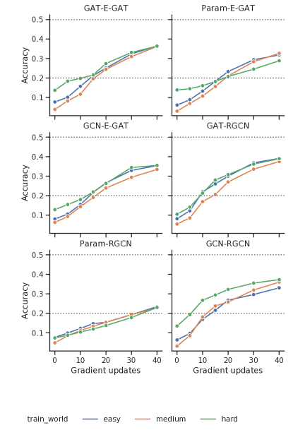
Figure 9: We evaluate the effect of $k$-shot adaptation on held out datasets when pre-trained on easy, medium and hard training datasets, among the different model architectures. Here, $k$ ranges from 0 to 40.

Using the notion of difficulty introduced in Section A.4, we perform the suite of experiments to evaluate the effect of pre-training on Easy, Medium and Difficult datasets. Interestingly, we find the performance on convergence is better on Medium and Hard datasets on pre-training, compared to the Easy dataset (Table 5). This behaviour is also mirrored in k-shot adaptation performance (Figure 9), where pre-training on Hard dataset provides faster adaptation performance on 4/6 models.

Appendix D Continual Learning

A natural question arises following our continual learning experiments in Section 5.3 : does the order of difficulty of the worlds matter? Thus, we perform an experiment following Curriculum Learning (Bengio et al., 2009) setup, where the order of the worlds being trained is determined by their relative difficulty (which is determined by the performance of models in supervised learning setup, Table 6, i.e., we order the worlds from easier worlds to harder worlds). We observe that while the current task accuracy follows the trend of the difficulty of the worlds (Figure 10), the mean of past accuracy is significantly worse. This suggests that a curriculum learning strategy might not be optimal to learn graph representations in a continual learning setting. We also performed the same experiment with sharing only the composition and representation functions (Figure 11), and observe similar trends where sharing the representation function reduces the effect of catastrophic forgetting.

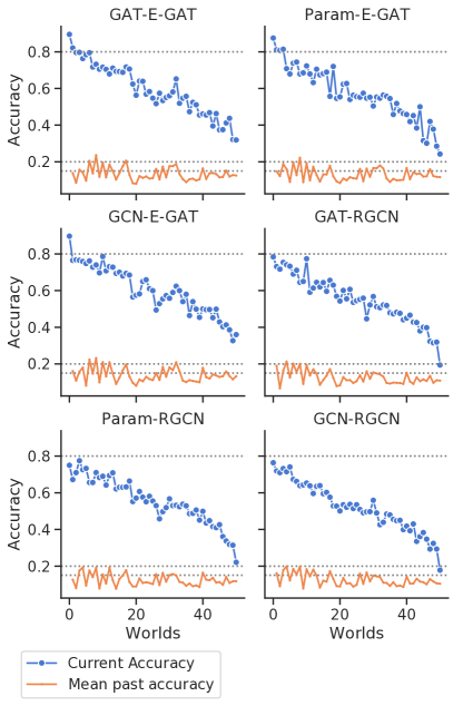
Figure 10: Curriculum Learning strategy in Continual Learning setup of GraphLog.

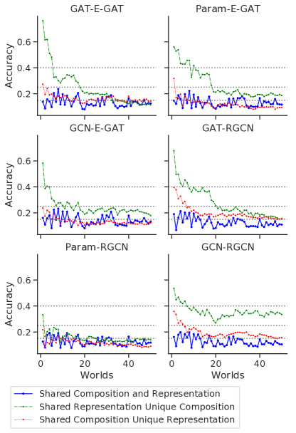
Figure 11: Curriculum Learning strategy in Continual Learning setup of GraphLog, when either the composition function or the representation function is shared for all worlds.

World ID	NC	ND	Split	ARL	AN	AE	D	M1	M2	M3	M4	M5	M6
rule_0	17	286	train	4.49	15.487	19.295	Hard	0.481	0.500	0.494	0.486	0.462	0.462
rule_1	15	239	train	4.10	11.565	13.615	Hard	0.432	0.411	0.428	0.406	0.400	0.408
rule_2	17	157	train	3.21	9.809	11.165	Hard	0.412	0.357	0.373	0.347	0.347	0.319
rule_3	16	189	train	3.63	11.137	13.273	Hard	0.429	0.404	0.473	0.373	0.401	0.451
rule_4	16	189	train	3.94	12.622	15.501	Medium	0.624	0.606	0.619	0.475	0.481	0.595
rule_5	14	275	train	4.41	14.545	18.872	Hard	0.526	0.539	0.548	0.429	0.461	0.455
rule_6	16	249	train	5.06	16.257	20.164	Hard	0.528	0.514	0.536	0.498	0.495	0.476
rule_7	17	288	train	4.47	13.161	16.333	Medium	0.613	0.558	0.598	0.487	0.486	0.537
rule_8	15	404	train	5.43	15.997	19.134	Medium	0.627	0.643	0.629	0.523	0.563	0.569
rule_9	19	1011	train	7.22	24.151	32.668	Easy	0.758	0.744	0.739	0.683	0.651	0.623
rule_10	18	524	train	5.87	18.011	22.202	Medium	0.656	0.654	0.663	0.596	0.563	0.605
rule_11	17	194	train	4.29	11.459	13.037	Medium	0.552	0.525	0.533	0.445	0.456	0.419
rule_12	15	306	train	4.14	11.238	12.919	Easy	0.771	0.726	0.603	0.511	0.561	0.523
rule_13	16	149	train	3.58	11.238	13.549	Hard	0.453	0.402	0.419	0.347	0.298	0.344
rule_14	16	224	train	4.14	11.371	13.403	Hard	0.448	0.457	0.401	0.314	0.318	0.332
rule_15	14	224	train	3.82	12.661	15.105	Hard	0.494	0.423	0.501	0.402	0.397	0.435
rule_16	16	205	train	3.59	11.345	13.293	Hard	0.318	0.332	0.292	0.328	0.306	0.291
rule_17	17	147	train	3.16	8.163	8.894	Hard	0.347	0.308	0.274	0.164	0.161	0.181
rule_18	18	923	train	6.63	25.035	33.080	Easy	0.700	0.680	0.713	0.650	0.641	0.618
rule_19	16	416	train	6.10	17.180	20.818	Easy	0.790	0.774	0.777	0.731	0.729	0.702
rule_20	20	2024	train	8.63	34.059	45.985	Easy	0.830	0.799	0.854	0.756	0.741	0.750
rule_21	13	272	train	4.58	10.559	11.754	Medium	0.621	0.610	0.632	0.531	0.516	0.580
rule_22	17	422	train	5.21	16.540	20.681	Medium	0.586	0.593	0.628	0.530	0.506	0.573
rule_23	15	383	train	4.97	17.067	21.111	Hard	0.508	0.522	0.493	0.455	0.473	0.476
rule_24	18	879	train	6.33	21.402	26.152	Easy	0.706	0.704	0.743	0.656	0.641	0.638
rule_25	15	278	train	3.84	11.093	12.775	Hard	0.424	0.419	0.382	0.358	0.345	0.412
rule_26	15	352	train	4.71	14.157	17.115	Medium	0.565	0.534	0.532	0.466	0.461	0.499
rule_27	16	393	train	4.98	14.296	16.499	Easy	0.713	0.714	0.722	0.632	0.604	0.647
rule_28	16	391	train	4.82	17.551	21.897	Medium	0.575	0.564	0.571	0.503	0.499	0.552
rule_29	16	144	train	3.87	10.193	11.774	Hard	0.468	0.445	0.475	0.325	0.336	0.389
rule_30	17	177	train	3.51	10.270	11.764	Hard	0.381	0.426	0.382	0.357	0.316	0.336
rule_31	19	916	train	5.90	20.147	26.562	Easy	0.788	0.789	0.770	0.669	0.674	0.641
rule_32	16	287	train	4.66	16.270	20.929	Medium	0.674	0.671	0.700	0.621	0.594	0.615
rule_33	18	312	train	4.50	14.738	18.266	Medium	0.695	0.660	0.709	0.710	0.679	0.668
rule_34	18	504	train	5.00	15.345	18.614	Easy	0.908	0.888	0.906	0.768	0.762	0.811
rule_35	19	979	train	6.23	21.867	28.266	Easy	0.831	0.750	0.782	0.680	0.700	0.662
rule_36	19	252	train	4.66	13.900	16.613	Easy	0.742	0.698	0.698	0.659	0.627	0.651
rule_37	17	260	train	4.00	11.956	14.010	Easy	0.843	0.826	0.826	0.673	0.698	0.716
rule_38	17	568	train	5.21	15.305	20.075	Easy	0.748	0.762	0.733	0.644	0.630	0.719
rule_39	15	182	train	3.98	12.552	14.800	Easy	0.737	0.642	0.635	0.592	0.603	0.587
rule_40	17	181	train	3.69	11.556	14.437	Medium	0.552	0.584	0.575	0.525	0.472	0.479
rule_41	15	113	train	3.58	10.162	11.553	Medium	0.619	0.601	0.626	0.490	0.468	0.470
rule_42	14	95	train	2.96	8.939	9.751	Hard	0.511	0.472	0.483	0.386	0.393	0.395
rule_43	16	162	train	3.36	11.077	13.337	Medium	0.622	0.567	0.579	0.473	0.482	0.437
rule_44	18	705	train	4.75	15.310	18.172	Hard	0.538	0.561	0.603	0.498	0.519	0.450
rule_45	15	151	train	3.39	9.127	10.001	Medium	0.569	0.580	0.592	0.535	0.524	0.524
rule_46	19	2704	train	7.94	31.458	43.489	Easy	0.850	0.820	0.828	0.773	0.762	0.749
rule_47	18	647	train	6.66	22.139	27.789	Easy	0.723	0.667	0.708	0.620	0.649	0.611
rule_48	16	978	train	6.15	17.802	21.674	Easy	0.812	0.798	0.812	0.772	0.763	0.753
rule_49	14	169	train	3.41	9.983	11.177	Easy	0.714	0.734	0.700	0.511	0.491	0.615
rule_50	16	286	train	3.99	12.274	16.117	Medium	0.651	0.653	0.656	0.555	0.583	0.570
rule_51	16	332	valid	4.44	16.384	21.817	Easy	0.746	0.742	0.738	0.667	0.657	0.689
rule_52	17	351	valid	4.81	16.231	20.613	Medium	0.697	0.716	0.754	0.653	0.655	0.670
rule_53	15	165	valid	3.65	10.838	12.378	Hard	0.458	0.464	0.525	0.334	0.364	0.373
rule_54	13	303	test	5.25	13.503	15.567	Medium	0.638	0.623	0.603	0.587	0.586	0.555
rule_55	16	293	test	4.83	16.444	20.944	Medium	0.625	0.582	0.578	0.561	0.528	0.571
rule_56	15	241	test	4.40	14.010	16.702	Medium	0.653	0.681	0.692	0.522	0.513	0.550
AGG	16.33	428.94		4.70	14.89	18.37		0.618 / 26	0.603 / 10	0.611 / 20	0.530 / 1	0.526 / 0	0.539 / 0

Table 6: Results on Single-task supervised setup for all datasets in GraphLog. Abbreviations: NC: Number of Classes, ND: Number of Descriptors, ARL: Average Resolution Length, AN: Average number of nodes, AE: Average number of edges

, D: Difficulty, AGG: Aggregate Statistics. List of models considered : M1: GAT-EGAT, M2: GCN-E-GAT, M3: Param-E-GAT, M4: GAT-RGCN, M5: GCN-RGCN and M6: Param-RGCN. Difficulty is calculated by taking the scores of the model (M1) and partitioning the worlds according to their accuracy ($\geq 0.7$ = Easy, $\geq 0.54$ and $<0.7$ = Medium, and $<0.54$ = Hard). We provide both the mean of the raw accuracy scores for all models, as well as the number of times the model is ranked first in all the tasks.

Appendix E Hyperparameters and Experimental Setup

In this section, we provide detailed hyperparameter settings for both models and dataset generation for the purposes of reproducibility. The codebase and dataset used in the experiments are attached with the Supplementary materials, and will be made public on acceptance.

E.1 Dataset Hyperparams

We generate GraphLog with 20 relations or classes ($K$), which results in 76 rules in $\mathcal{R_{S}}$ after consistency checks. For unary rules, we specify half of the relations to be symmetric and other half to have their invertible relations. To split the rules for individual worlds, we choose the number of rules for each world $w=20$ and stride $s=1$, and end up with 57 worlds $\mathcal{R}_{0}\ldots\mathcal{R}_{56}$. For each world $\mathcal{R}_{i}$, we generate 5000 training, 1000 testing and 1000 validation graphs.

E.2 Model Hyperparams

For all models, we perform hyper-parameter sweep (grid search) to find the optimal values based on the validation accuracy. For all models, we use the relation embedding and node embedding to be 200 dimensions. We train all models with Adam optimizer with learning rate 0.001 and weight decay of 0.0001. For supervised setting, we train all models for 500 epochs, and we add a scheduler for learning rate to decay it by 0.8 whenever the validation loss is stagnant for 10 epochs. In multitask setting, we sample a new task every epoch from the list of available tasks. Here, we run all models for 2000 epochs when we have the number of tasks $\leq 10$. For larger number of tasks (Figure 4), we train by proportionally increasing the number of epochs compared to the number of tasks. (2k epochs for 10 tasks, 4k epochs for 20 tasks, 6k epochs for 30 tasks, 8k epochs for 40 tasks and 10k epochs for 50 tasks). For continual learning experiment, we train each task for 100 epochs for all models. No learning rate scheduling is used for either multitask or continual learning experiments. Individual model hyper-parameters are as follows:

• Representation functions :

  • GAT : Number of layers = 2, Number of attention heads = 2, Dropout = 0.4

  • GCN : Number of layers = 2, with symmetric normalization and bias, no dropout

• Composition functions:

  • E-GAT: Number of layers = 6, Number of attention heads = 2, Dropout = 0.4

  • RGCN: Number of layers = 2, no dropout, with bias.

References

- Alexander (2016) Alexander, P. A. Relational thinking and relational reasoning: harnessing the power of patterning. NPJ science of learning, 1(1):1–7, 2016.
- Bahdanau et al. (2018) Bahdanau, D., Murty, S., Noukhovitch, M., Nguyen, T. H., de Vries, H., and Courville, A. Systematic generalization: what is required and can it be learned? arXiv preprint arXiv:1811.12889, 2018.
- Battaglia et al. (2016) Battaglia, P., Pascanu, R., Lai, M., Rezende, D. J., et al. Interaction networks for learning about objects, relations and physics. In Advances in neural information processing systems, pp. 4502–4510, 2016.
- Battaglia et al. (2018) Battaglia, P. W., Hamrick, J. B., Bapst, V., Sanchez-Gonzalez, A., Zambaldi, V., Malinowski, M., Tacchetti, A., Raposo, D., Santoro, A., Faulkner, R., et al. Relational inductive biases, deep learning, and graph networks. arXiv preprint arXiv:1806.01261, 2018.
- Bengio et al. (2009) Bengio, Y., Louradour, J., Collobert, R., and Weston, J. Curriculum learning. In Proceedings of the 26th annual international conference on machine learning, pp. 41–48, 2009.
- Bordes et al. (2013) Bordes, A., Usunier, N., Garcia-Duran, A., Weston, J., and Yakhnenko, O. Translating embeddings for modeling multi-relational data. In Advances in neural information processing systems, pp. 2787–2795, 2013.
- Chen et al. (2019) Chen, T., Bian, S., and Sun, Y. Are powerful graph neural nets necessary? a dissection on graph classification. arXiv preprint arXiv:1905.04579, 2019.
- Côté et al. (2018) Côté, M.-A., Kádár, Á., Yuan, X., Kybartas, B., Barnes, T., Fine, E., Moore, J., Hausknecht, M., El Asri, L., Adada, M., et al. Textworld: A learning environment for text-based games. In Workshop on Computer Games, pp. 41–75. Springer, 2018.
- De Lange et al. (2019) De Lange, M., Aljundi, R., Masana, M., Parisot, S., Jia, X., Leonardis, A., Slabaugh, G., and Tuytelaars, T. Continual learning: A comparative study on how to defy forgetting in classification tasks. arXiv preprint arXiv:1909.08383, 2019.
- Defferrard et al. (2016) Defferrard, M., Bresson, X., and Vandergheynst, P. Convolutional neural networks on graphs with fast localized spectral filtering. In Advances in neural information processing systems, pp. 3844–3852, 2016.
- Dijkstra (1982) Dijkstra, E. W. On the role of scientific thought. In Selected writings on computing: a personal perspective, pp. 60–66. Springer, 1982.
- Du et al. (2019) Du, S. S., Hou, K., Salakhutdinov, R. R., Poczos, B., Wang, R., and Xu, K. Graph neural tangent kernel: Fusing graph neural networks with graph kernels. In Advances in Neural Information Processing Systems, pp. 5724–5734, 2019.
- Duvenaud et al. (2015) Duvenaud, D. K., Maclaurin, D., Iparraguirre, J., Bombarell, R., Hirzel, T., Aspuru-Guzik, A., and Adams, R. P. Convolutional networks on graphs for learning molecular fingerprints. In Advances in neural information processing systems, pp. 2224–2232, 2015.
- Evans & Grefenstette (2017) Evans, R. and Grefenstette, E. Learning Explanatory Rules from Noisy Data. November 2017.
- Farrington-Flint et al. (2007) Farrington-Flint, L., Canobi, K. H., Wood, C., and Faulkner, D. The role of relational reasoning in children’s addition concepts. British Journal of Developmental Psychology, 25(2):227–246, 2007.
- Gilmer et al. (2017) Gilmer, J., Schoenholz, S. S., Riley, P. F., Vinyals, O., and Dahl, G. E. Neural message passing for quantum chemistry. In Proceedings of the 34th International Conference on Machine Learning-Volume 70, pp. 1263–1272. JMLR. org, 2017.
- Guo et al. (2018) Guo, M., Haque, A., Huang, D.-A., Yeung, S., and Fei-Fei, L. Dynamic task prioritization for multitask learning. In Proceedings of the European Conference on Computer Vision (ECCV), pp. 270–287, 2018.
- Guo et al. (2016) Guo, S., Wang, Q., Wang, L., Wang, B., and Guo, L. Jointly embedding knowledge graphs and logical rules. In Proceedings of the 2016 Conference on Empirical Methods in Natural Language Processing, pp. 192–202, 2016.
- Halford et al. (2010) Halford, G. S., Wilson, W. H., and Phillips, S. Relational knowledge: the foundation of higher cognition. Trends in cognitive sciences, 14(11):497–505, 2010.
- Hamilton et al. (2017a) Hamilton, W., Ying, R., and Leskovec, J. Representation learning on graphs: Methods and applications. IEEE Data Engineering Bulletin, 2017a.
- Hamilton et al. (2017b) Hamilton, W., Ying, Z., and Leskovec, J. Inductive representation learning on large graphs. In Advances in neural information processing systems, pp. 1024–1034, 2017b.
- Hamilton et al. (2018) Hamilton, W., Bajaj, P., Zitnik, M., Jurafsky, D., and Leskovec, J. Embedding logical queries on knowledge graphs. In Advances in Neural Information Processing Systems 31, pp. 2026–2037. 2018.
- Hochreiter & Schmidhuber (1997) Hochreiter, S. and Schmidhuber, J. Long short-term memory. Neural computation, 9(8):1735–1780, 1997.
- Hoffart et al. (2011) Hoffart, J., Suchanek, F. M., Berberich, K., Lewis-Kelham, E., De Melo, G., and Weikum, G. Yago2: exploring and querying world knowledge in time, space, context, and many languages. In Proceedings of the 20th international conference companion on World wide web, pp. 229–232, 2011.
- Holyoak & Morrison (2012) Holyoak, K. J. and Morrison, R. G. The Oxford handbook of thinking and reasoning. Oxford University Press, 2012.
- Johnson et al. (2017) Johnson, J., Hariharan, B., van der Maaten, L., Fei-Fei, L., Lawrence Zitnick, C., and Girshick, R. Clevr: A diagnostic dataset for compositional language and elementary visual reasoning. In Proceedings of the IEEE Conference on Computer Vision and Pattern Recognition, pp. 2901–2910, 2017.
- Kipf & Welling (2016) Kipf, T. N. and Welling, M. Semi-supervised classification with graph convolutional networks. arXiv preprint arXiv:1609.02907, 2016.
- Krawczyk et al. (2011) Krawczyk, D. C., McClelland, M. M., and Donovan, C. M. A hierarchy for relational reasoning in the prefrontal cortex. Cortex, 47(5):588–597, 2011.
- Lake & Baroni (2017) Lake, B. M. and Baroni, M. Generalization without systematicity: On the compositional skills of sequence-to-sequence recurrent networks. arXiv preprint arXiv:1711.00350, 2017.
- Langley & Simon (1995) Langley, P. and Simon, H. A. Applications of machine learning and rule induction. Communications of the ACM, 38(11):54–64, 1995.
- Mahdisoltani et al. (2013) Mahdisoltani, F., Biega, J., and Suchanek, F. M. Yago3: A knowledge base from multilingual wikipedias. 2013.
- Miller (1995) Miller, G. A. Wordnet: a lexical database for english. Communications of the ACM, 38(11):39–41, 1995.
- Mitchell & Fredkin (2014) Mitchell, T. and Fredkin, E. Never ending language learning. In Big Data (Big Data), 2014 IEEE International Conference on, pp. 1–1, 2014.
- Morris et al. (2019) Morris, C., Ritzert, M., Fey, M., Hamilton, W., Lenssen, J., Rattan, G., and Grohe, M. Weisfeiler and Leman go neural: Higher-order graph neural networks. In AAAI, 2019.
- Parisi et al. (2019) Parisi, G. I., Kemker, R., Part, J. L., Kanan, C., and Wermter, S. Continual lifelong learning with neural networks: A review. Neural Networks, 2019.
- Paszke et al. (2019) Paszke, A., Gross, S., Massa, F., Lerer, A., Bradbury, J., Chanan, G., Killeen, T., Lin, Z., Gimelshein, N., Antiga, L., Desmaison, A., Kopf, A., Yang, E., DeVito, Z., Raison, M., Tejani, A., Chilamkurthy, S., Steiner, B., Fang, L., Bai, J., and Chintala, S. Pytorch: An imperative style, high-performance deep learning library. In Wallach, H., Larochelle, H., Beygelzimer, A., dÁlché-Buc, F., Fox, E., and Garnett, R. (eds.), Advances in Neural Information Processing Systems 32, pp. 8024–8035. Curran Associates, Inc., 2019. URL http://papers.nips.cc/paper/9015-pytorch-an-imperative-style-high-performance-deep-learning-library.pdf.
- Paulheim (2017) Paulheim, H. Knowledge graph refinement: A survey of approaches and evaluation methods. Semantic web, 8(3):489–508, 2017.
- Richland et al. (2010) Richland, L. E., Chan, T.-K., Morrison, R. G., and Au, T. K.-F. Young children’s analogical reasoning across cultures: Similarities and differences. Journal of Experimental Child Psychology, 105(1-2):146–153, 2010.
- Santoro et al. (2017) Santoro, A., Raposo, D., Barrett, D. G., Malinowski, M., Pascanu, R., Battaglia, P., and Lillicrap, T. A simple neural network module for relational reasoning. In Advances in neural information processing systems, pp. 4967–4976, 2017.
- Santoro et al. (2018) Santoro, A., Faulkner, R., Raposo, D., Rae, J., Chrzanowski, M., Weber, T., Wierstra, D., Vinyals, O., Pascanu, R., and Lillicrap, T. Relational recurrent neural networks. In Advances in neural information processing systems, pp. 7299–7310, 2018.
- Scarselli et al. (2008) Scarselli, F., Gori, M., Tsoi, A. C., Hagenbuchner, M., and Monfardini, G. The graph neural network model. IEEE Transactions on Neural Networks, 20(1):61–80, 2008.
- Schlag et al. (2019) Schlag, I., Smolensky, P., Fernandez, R., Jojic, N., Schmidhuber, J., and Gao, J. Enhancing the transformer with explicit relational encoding for math problem solving. arXiv preprint arXiv:1910.06611, 2019.
- Schlichtkrull et al. (2018) Schlichtkrull, M., Kipf, T. N., Bloem, P., Van Den Berg, R., Titov, I., and Welling, M. Modeling relational data with graph convolutional networks. In European Semantic Web Conference, pp. 593–607. Springer, 2018.
- Sinha et al. (2019) Sinha, K., Sodhani, S., Dong, J., Pineau, J., and Hamilton, W. L. Clutrr: A diagnostic benchmark for inductive reasoning from text. arXiv preprint arXiv:1908.06177, 2019.
- Sodhani et al. (2019) Sodhani, S., Chandar, S., and Bengio, Y. On training recurrent neural networks for lifelong learning. 2019.
- Son et al. (2011) Son, J. Y., Smith, L. B., and Goldstone, R. L. Connecting instances to promote children’s relational reasoning. Journal of experimental child psychology, 108(2):260–277, 2011.
- Suchanek et al. (2007) Suchanek, F. M., Kasneci, G., and Weikum, G. Yago: a core of semantic knowledge. In Proceedings of the 16th international conference on World Wide Web, pp. 697–706, 2007.
- Thrun & Pratt (2012) Thrun, S. and Pratt, L. Learning to learn. Springer Science & Business Media, 2012.
- Vaswani et al. (2017) Vaswani, A., Shazeer, N., Parmar, N., Uszkoreit, J., Jones, L., Gomez, A. N., Kaiser, Ł., and Polosukhin, I. Attention is all you need. In Advances in neural information processing systems, pp. 5998–6008, 2017.
- Veličković et al. (2017) Veličković, P., Cucurull, G., Casanova, A., Romero, A., Lio, P., and Bengio, Y. Graph attention networks. arXiv preprint arXiv:1710.10903, 2017.
- West et al. (2014) West, R., Gabrilovich, E., Murphy, K., Sun, S., Gupta, R., and Lin, D. Knowledge base completion via search-based question answering. In Proceedings of the 23rd international conference on World wide web, pp. 515–526, 2014.
- Xu et al. (2018) Xu, K., Hu, W., Leskovec, J., and Jegelka, S. How powerful are graph neural networks? arXiv preprint arXiv:1810.00826, 2018.
- Ying et al. (2019) Ying, Z., Bourgeois, D., You, J., Zitnik, M., and Leskovec, J. Gnnexplainer: Generating explanations for graph neural networks. In Advances in Neural Information Processing Systems, pp. 9240–9251, 2019.