Electro-osmotic properties of porous permeable films

Abstract

Permeable porous coatings on a flat solid support significantly impact its electrostatic and electrokinetic properties. Existing work has focused on simplified cases, such as weakly charged and/or thick porous films, with limited theoretical guidance. Here, we consider the general case of coatings of an arbitrary volume charge density and obtain analytic formulas for electrostatic potential profiles, valid for any film thickness and salt concentration. Our analysis provides a framework for interpreting and predicting super properties specific to porous films, from an enhanced ion absorption to a consequent amplification of electro-osmotic flows due to emergence of slip velocity at interface with an outer electrolyte leading to a large zeta-potential. The latter can be tuned by varying amount of added salt, and remains finite at even high concentrations. The results are relevant for hydrogel coatings, porous carbon and silica, polyelectrolyte brushes, and more.

I Introduction

Charged porous materials that are permeable to water and ions, such as polyelectrolyte networks, ion-exchange resins, silica gels, porous membranes and electrodes, have found use in a large body of applications including water desalination Porada et al. (2012), tissue engineering Stamatialis et al. (2008); Chung et al. (2018), and electrochemical systems Biesheuvel et al. (2011). Thanks to a recently discovered extremely strong electrokinetic flow near porous surfaces Feldmann et al. (2020), new opportunities in microfluidics and advanced colloid technologies are emerging. Porous films on a variety of supports, are similarly capable to provide such properties as improved transport and storage capacities for ions, that they did not have when impermeable. However, the quantitative understanding of novel equilibrium and transport properties, which could not be achieved without porosity is still challenging.

A considerable progress has been made over the last decades in understanding the equilibrium properties of porous surfaces in electrolyte solutions. Analytic solutions based on a linearized Poisson-Boltzmann theory are known Donath and Pastushenko (1979); Ohshima and Ohki (1985); Ohshima and Kondo (1990); Chanda et al. (2014), but these results do not apply to highly charged coatings, where nonlinear electrostatic effects could become significant. The non-linear electrostatic problem has been treated using numeric and semi-analytic approaches Ohshima and Ohki (1985); Duval (2005); Chen and Das (2015), and some simple analytic expressions for the static surface potential, $\Psi_{s}$ have been derived for thick coatings compared to the Debye screening length, $\lambda_{D}$, which is a measure of the thickness of the electrostatic diffuse layer Ohshima and Ohki (1985); Silkina et al. (2020). Nevertheless, approaches to calculate $\Psi_{s}$ analytically are sill lacking and general principles to control it have not yet been established, especially for the case of strongly charged coatings of a thickness smaller or comparable to $\lambda_{D}$.

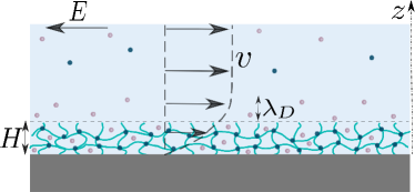
Figure 1: Porous film of thickness $H$ in contact with an electrolyte solution. Anions and cations are denoted with bright and dark circles. An outer electrostatic diffuse layer of a thickness of the order of $\lambda_{D}\equiv\kappa^{-1}$, is formed in the vicinity of the coating. A tangential electric field, $E$, leads to a solvent flow of velocity $v$ (shown by right arrows).

The electro-kinetic properties of porous surfaces in electrolyte solutions are relatively less understood, although there is some literature describing attempts to provide a theory of electro-osmosis near porous surfaces. It has been understood that $\Psi_{s}$ of porous surfaces does not define unambiguously the electro-osmotic flow properties Donath and Pastushenko (1979), and that bulk velocity is controlled, besides $\Psi_{s}$, by the Brinkman and inner Debye screening lengths Ohshima and Kondo (1990). These authors, however, failed to propose a physical interpretation of their results, which generally indicate that porous surfaces can amplify electro-osmotic pumping at micron scales, where pressure-driven flows are suppressed by viscosity. These theories and subsequent attempts at improvement the description of the electroosmosis near porous surfaces Ohshima (1995); Duval and van Leeuwen (2004); Duval (2005); Ohshima (2006) are often invoked in the interpretation of the electro-osmotic data, but their relation to electrokinetic (zeta) potential, $Z$, which is the measure of electrokinetic mobility, has remained somewhat obscure. Some authors concluded that it ‘loses its significance’ Ohshima and Kondo (1990) or ‘is undefined and thus nonapplicable’ Duval and van Leeuwen (2004), while others reported that $Z$ typically exceeds $\Psi_{s}$ Sobolev et al. (2017); Chen and Das (2015), but did not attempt to relate their results to the inner flow and emerging liquid velocity at the interface. Besides, neither paper attempted to understand an upper bound on achievable zeta-potential. We, therefore, gained the impression that certain crucial aspects of the electrokinetics near the porous interface are either poorly understood or have been given so far insufficient attention.

In this paper, we describe analytically the distribution of a potential induced by a planar porous coating. Our simple analytic expressions are valid even when the volume charge density is quite large, and can be used for any salt concentration and thickness of a porous layer. From this theory, we are interpreting enhanced absorption properties of porous films, and show that due to these mobile absorbed ions the electro-osmotic flow inside the porous film emerges, which in turns leads to the finite slip velocity at the porous interface. The later is the reason for an enhancement of the electro-osmotic velocity in the bulk electrolyte and of zeta-potential. Finally, we obtain an upper bound on attainable zeta-potential that provides guidance for a giant amplification of electro-osmotic flows.

II Electro-osmotic equilibria

The system geometry is shown in Fig. 1. The permeable film of a thickness $H$ and a fixed volume charge density $\varrho$ (taken positive without loss of generality) is placed in an 1:1 electrolyte solution of bulk concentration $c_{\infty}$ and permittivity $\varepsilon$. Ions obey Boltzmann distribution, $c_{\pm}(z)=c_{\infty}\exp(\mp\psi(z))$, where $\psi(z)=e\Psi(z)/(k_{B}T)$ is the dimensionless electrostatic potential, $e$ is the elementary positive charge, $k_{B}$ is the Boltzmann constant, $T$ is a temperature, and the upper (lower) sign corresponds to the cations (anions). The inverse Debye screening length of an electrolyte solution, $\kappa\equiv\lambda_{D}^{-1}$, is defined as usually, $\kappa^{2}=8\pi\ell_{B}c_{\infty}$, with the Bjerrum length $\ell_{B}=\dfrac{e^{2}}{\varepsilon k_{B}T}$.

II.1 Electrostatic Potentials

To calculate the profile of a potential inside the porous film and in the outer solution we employ the nonlinear Poisson-Boltzmann theory Andelman (1995), so that $\psi(z)$ satisfies

$$\psi_{i,o}^{{}^{\prime\prime}}=\kappa^{2}\left(\sinh\psi_{i,o}-\rho\Theta\left(H-z\right)\right),$$ (1)

where ^′ denotes $d/dz$, with the index $\{i,o\}$ standing for “in” $(z\leq H)$ and “out” $(z\geq H)$, $\rho=\dfrac{\varrho}{2ec_{\infty}}$, and the Heaviside step function $\Theta(z)$. The solution of non-linear Eq.(1) with prescribed boundary conditions, in general requires a numerical method. Here we obtain a closed-form analytical solution.

Integrating Eq.(1) twice by applying conditions $\psi_{o}^{{}^{\prime}}\rightarrow 0$ and $\psi_{o}\rightarrow 0$ at $z\rightarrow\infty$ we naturally find that the $\psi_{o}-$profile is identical to derived for an impenetrable wall Andelman (1995)

$$\psi_{o}=4\operatorname{artanh}\left[\gamma e^{-\kappa(z-H)}\right]$$ (2)

where $\gamma=\tanh\dfrac{\psi_{s}}{4}$ and $\psi_{s}=\psi(H)$ is the surface potential. Using $\psi_{i}^{{}^{\prime}}(0)=0$ and $\psi_{i}(0)=\psi_{0}$ we obtain that $\psi_{0}$ and $\psi_{s}$ are related as

$$\psi_{s}\equiv\psi_{0}-\frac{\cosh\psi_{0}-1}{\rho},$$ (3)

derived before for thick films only Silkina et al. (2020). Note that Eqs.(3) and (2), are exact and valid for any $\kappa H$ and $\rho$.

Further insight can be gained by recalling that $\cosh\psi$ represents a dimensionless local osmotic pressure of an electrolyte solution, $p=P/2c_{\infty}k_{B}T$, which takes its largest value of $p_{0}=\cosh\psi_{0}$ at $z=0$. Since $p(\infty)=1$, Eq.(3) indicates that an excess osmotic pressure at the wall grows linearly with a self-induced potential difference across the porous film, $\psi_{0}-\psi_{s}$. It will be clear below that this is a main parameter that ascertains most of its properties.

In the limit of a thin film, $\kappa H\ll 1$, the asymptotic approach suggested before Silkina et al. (2019) can be employed. Expanding the potential in Eq.(1) about $z=0$, we obtain, to second order in $\kappa z$

$$\psi_{i}(z)\simeq\psi_{0}-\dfrac{\rho}{2}\left(\kappa z\right)^{2}\left[1-\frac{\sinh\psi_{0}}{\rho}\right].$$ (4)

Note that the value of $\sinh\left(\psi_{0}\right)/\rho\leq 1$ represents the degree of screening of the film intrinsic charge at $z=0$.

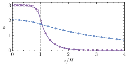
Figure 2: A distribution of a potential built up by a film of $\rho=10$, calculated numerically for $\kappa H=0.3$ (dashed curve) and $3$ (solid curve). Filled circles correspond to calculations from Eqs.(10), (14), when $z/H\leq 1$, and from Eq.(2), when $z/H\geq 1$. Open squares are obtained from Eq.(15).

From Eqs.(4) and (3) it follows that $\psi_{0}$ satisfies

$$\rho^{2}-\rho\sinh\psi_{0}-\frac{2\left(\cosh\psi_{0}-1\right)}{(\kappa H)^{2}}\simeq 0,$$ (5)

and standard manipulations then yield

$$\psi_{0}\simeq\ln\left[\frac{2+(\rho\kappa H)^{2}+\rho\kappa H\sqrt{4+(\kappa H)^{2}(1+\rho^{2})}}{2+\rho(\kappa H)^{2}}\right]$$ (6)

For sufficiently large $\rho$, this may be reexpressed as

$$\psi_{0}\simeq\ln\left[\frac{\left(\dfrac{\rho\kappa H}{2}+\sqrt{1+\left(\dfrac{\rho\kappa H}{2}\right)^{2}}\right)^{2}}{1+\dfrac{\rho(\kappa H)^{2}}{2}}\right],$$ (7)

which is equivalent to

$$\psi_{0}\simeq 2\operatorname{arsinh}\left(\dfrac{\rho\kappa H}{2}\right)-\ln\left(1+\dfrac{\rho(\kappa H)^{2}}{2}\right).$$ (8)

For small $\rho\kappa H$, the $\psi$-profile is almost constant throughout the film,

$$\psi_{0}\simeq\psi_{s}\simeq\rho\kappa H,$$ (9)

as follows directly from (6).

Finally, the inner $\psi$-profile of a thin film is given by

$$\psi_{i}(z)\simeq\psi_{s}-\frac{\left[\sinh\psi_{0}-\rho\right]}{2}\kappa^{2}(H^{2}-z^{2}),$$ (10)

where $\psi_{s}$ and $\psi_{0}$ are described by Eqs.(3) and (8).

The startling conclusion from analysis of Eq.(5) is that it is also valid for $\kappa H\gg 1$, i.e. thick films, where the inner region far from the interface may be modeled as electroneutral. Indeed, in this case the last term on its left-hand side becomes very small compared with the first two, and we obtain a well-known for thick films result Ohshima and Ohki (1985)

$$\psi_{0}=\operatorname{arsinh}(\rho),$$ (11)

which leads to $p_{0}=\sqrt{1+\rho^{2}}$. The potential of an electroneutral area of a thick film is usually referred to as the Donnan potential, $\psi_{D}$, so that Eq.(11) relates $\psi_{D}$ with $\rho$. Note that in this limit Eq.(3) can be transformed to

$$\psi_{s}=\psi_{0}+\displaystyle\frac{1-\sqrt{1+\rho^{2}}}{\rho}$$ (12)

Near the surface electrolyte ions screen volume charges of the coating only partly, and an inner diffuse layer is formed. The inverse inner screening length can be found as

$$\kappa_{i}=\kappa(\cosh{\psi_{0}})^{1/2}\equiv\kappa\sqrt{p_{0}}$$ (13)

From Eq.(11) it then follows that $\kappa_{i}\simeq\kappa(1+\rho^{2})^{1/4}$, which indicates that when $\rho\ll 1$, a sensible approximation should be $\kappa_{i}\simeq\kappa$. However, when $\rho\gg 1$, $\kappa_{i}\simeq\kappa\sqrt{\rho}$, and the criterion of a thick film can be relaxed to $\kappa H\sqrt{\rho}\gg 1$.

Since the thick film ‘behaves’ as an electrolyte solution of the inverse Debye length $\kappa_{i}$, to obtain the exact equation for $\psi_{i}$ it is enough to simply change the variables in Eq.(2). Namely, substitution of $z$ by $-z$, $\psi_{s}$ by $\psi_{0}-\psi_{s}$, and $\psi_{o}$ by $\psi_{0}-\psi_{i}$ would immediately give

$$\psi_{0}-\psi_{i}=4\operatorname{artanh}\left[\gamma_{i}e^{-\kappa_{i}(H-z)}\right],$$ (14)

where $\gamma_{i}=\tanh{\dfrac{\psi_{0}-\psi_{s}}{4}}$. Using Eqs.(11) and (12) we obtain $\gamma_{i}=\tanh\left({\dfrac{\sqrt{1+\rho^{2}}-1}{4\rho}}\right)$, which reduces to $\gamma_{i}\simeq\rho/8$ if $\rho\ll 1$, and $\gamma_{i}\simeq\dfrac{1}{4}\left(1-\dfrac{1}{\rho}\right)$ when $\rho\gg 1$. This implies that $\gamma_{i}$ is always smaller than 1/4. For such a small $\gamma_{i}$, the inner potential can be expanded about $\psi_{0}$, and to first order in $\psi_{0}-\psi_{s}$ we obtain

$$\psi_{i}(z)\simeq\psi_{0}+(\psi_{s}-\psi_{0})e^{\kappa_{i}(z-H)}$$ (15)

This derivation differs from conventional arguments, which assume low volume charge density Ohshima and Ohki (1985). Our treatment clarifies that Eq.(15) constitutes a sensible approximation for $\psi_{i}$ of a thick film of any $\rho$.

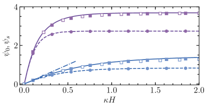
Figure 3: Potentials at wall (solid lines) and surface (dashed) as a function of $\kappa H$ computed for fixed $\rho=20$ (upper set of curves) and $\rho=2$ (lower curves). Filled squares illustrate calculations from Eq.(6), circles are then obtained using Eq.(3). Open squares show results obtained using Eq.(8). Dash-dotted line is calculated from Eq.(9).

In order to assess the validity of the above approach, we employ numerical simulations. We perform a numerical resolution of a multi-point boundary value problem for the nonlinear Poisson-Boltzmann differential equation Eq. (1) with prescribed boundary conditions, using the numerical approach based on the collocation method developed by Bader and Ascher (1987).

In Fig. 2 we plot $\psi(z/H)$ computed for two different values of $\kappa H$ that are close to limits of thick and thin films, and a large fixed $\rho$. The form of the $\psi$-profile depends on $\kappa H$. For $\kappa H=3$ the inner potential shows a distinct plateau indicating that the intrinsic charge of the film is completely screened by electrolyte ions, i.e. global electroneutrality. The plateau potential is equal to $\psi_{D}$. However, when $\kappa H=0.3$, there is no electroneutral region inside the film, and the potential at wall, $\psi_{0}$, is much smaller than $\psi_{D}$. Also included in Fig. 2 are theoretical results obtained from Eqs.(2), (10), (14), and (15) and we conclude that in relevant areas they are in excellent agreement with numerical data.

It is tempting to speculate that Eq.(6) will be applicable for any $\kappa H$, and that a more elegant result, Eq.(8), can be used provided $\rho$ large enough. Clearly, Eq.(5) could become less accurate for intermediate $\kappa H$, and it is of considerable interest to determine its regime of validity. To test ansatz Eq.(5), numerical and theoretical $\psi_{0}$ and $\psi_{s}$ have been calculated as a function of $\kappa H$ for different values of $\rho$. Specimen results are plotted in Fig. 3 confirming the validity of Eqs.(6) and (8) for all $\kappa H$. As expected, Eq.(9), which can also be obtained using the linear theory Ohshima and Ohki (1985), is valid only when $\rho\kappa H$ is very small and significantly overestimates potentials, which saturate at some $\kappa H$, in other cases. The charge density dependence of $\psi_{0}$ and $\psi_{s}$ is also of interest. Fig. 4 illustrates the weak growth of both potentials with $\rho$, and that $\psi_{0}-\psi_{s}\simeq 1$ as $\rho\kappa H$ is increased. We again conclude that Eq.(6) fits accurately the numerical data. So does (8), except for $\rho\leq 1$, where some very small discrepancy is observed. Below we use Eq.(8) for all calculations, by omitting a discussion of the accuracy of our theory.

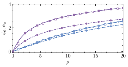
Figure 4: Potentials at wall (solid lines) and surface (dashed) as a function of $\rho$ computed for fixed $\kappa H=3$ (upper set of curves) and $\kappa H=0.2$ (lower curves). Filled squares illustrate calculations from Eq.(6), circles are then obtained using Eq.(3). Open squares show predictions of Eq.(8).

II.2 Ion concentrations

The problem we address here is the calculation of the profile of a cloud of counter-ions forming a diffuse electrostatic layer close to a planar surface of a porous film. Since ions obey Boltzmann distribution, their local concentration $c_{\pm}/c_{\infty}=\exp{(\mp\psi})$ are determined solely by the $\psi$-profile calculated above. Representative concentration profiles computed for highly charged porous films of $\rho=10$ and two different values of $\kappa H$ are shown in Fig. 5. We see that in the inner region anions are significantly enriched, and cations are depleted. The degree of this enrichment and depletion depends on the values of $\rho$ and $\kappa H$. At the given $\rho$ the degree of enrichment is ca.20 for a thick film of $kH=5$, but it is a few times smaller when $kH=0.2$. We also stress that for a chosen value of $\rho$ inner concentrations of cations practically vanish for both $\kappa H$.

To boost absorption of ions, coatings of larger $\rho$ can be used, as illustrated in Fig. 6, where the total concentration of ions at the wall, $c_{0}=c_{+}(0)+c_{-}(0),$ scaled by the sum of anion and cation concentrations at infinity, $2c_{\infty}$, is plotted as a function of $\rho$. We note that for a thick film $c_{0}\equiv p_{0}$, as follows from Eq. (11), so that it grows linearly with $\rho$, when it becomes large enough. Eq.(11) describes perfectly numerical data for $\kappa H=3$, and it is clear that this curve corresponds to an upper attainable value of ion-enrichment at the wall. In other words, the absorption capacity cannot be further improved by making the coating thicker. However, the reduction in $H$ could significantly reduce the concentration of absorbed anions, especially at $\rho\leq 10$.

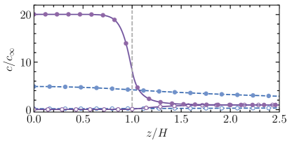
Figure 5: Ion concentration profiles computed at $\rho=10$ using $\kappa H=0.2$ (dashed curves) and $5$ (solid curves). Local concentrations of anions (filled circles) and cations (open circles) are calculated using Eq.(2) when $z/H\geq 1$, and from Eqs.(10) and Eq.(14) when $z/H\leq 1$.

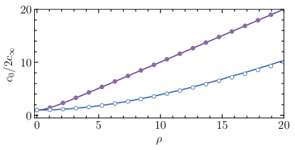
Figure 6: Ion-enrichment at the wall, $c_{0}/2c_{\infty}=\cosh\psi_{0}$, vs. $\rho$ computed using $\kappa H=3$ (upper curve) and $0.3$ (lower curve). Filled and open circles are obtained from Eqs.(11) and (6).

III Electroosmotic Velocity and zeta potential

Another relevant problem is an electro-osmotic flow of a solvent of the dynamic viscosity $\eta$ in an applied tangential electric field, $E$. The origin of the electro-osmotic flow is traditionally attributed to diffuse layers. Below we show that for porous coatings the electroosmosis is defined both by diffuse layers and the absorbed ions, and that the second mechanism is responsible for a flow amplification and dominates at high salt.

We are now about to relate the dimensionless velocity, $v(z)=\dfrac{4\pi\ell_{B}\eta}{eE}V(z)$, of such a flow to $\psi_{0}$ and $\psi_{s}$. We assume weak field, so that in steady state $\psi(z)$ is independent of the fluid flow. Note that for our planar geometry the concentration gradients at every location are perpendicular to the direction of the flow, it is therefore legitimate to neglect advection. Therefore, the liquid flow satisfies the generalized Stokes equation

$$v^{\prime\prime}-\mathcal{K}^{2}v\Theta(H-z)=\psi^{\prime\prime}+\kappa^{2}\rho\Theta(H-z),$$ (16)

where $\mathcal{K}$ is the inverse Brinkman length. At the wall we apply a classical no-slip condition, $v_{0}=v(0)=0$, and far from the surface $v^{\prime}_{z\rightarrow\infty}=0$. We consider the limits of small flow extension into the porous medium, $\mathcal{K}H\to\infty$, and of $\mathcal{K}H\to 0$, where an additional dissipation in the porous film can be neglected, to obtain bounds on the electro-osmotic velocity that constrain its attainable value.

From analysis of Eq.(16) it follows that the outer $v$-profile and velocity in the bulk are given by

$$v_{o}(z)=v_{\infty}+\psi_{o}(z),\,v_{\infty}=v_{s}-\psi_{s}=-\zeta,$$ (17)

where $\psi_{o}$ is defined by Eq.(2), $v_{s}=v(H)$ is the liquid velocity at surface, below we refer it to as slip velocity, and $\zeta=eZ/(k_{B}T)$. Eqs.(17) indicate that enhanced electro-osmotic mobility can be a consequence of large equilibrium $\psi_{s}$, as well as of large $v_{s}$ that depends on the hydrodynamic permeability of the coating. The amplification of the electro-osmotic flow (compared to the no-slip case with the same $\psi_{s}$) can be expressed as

$$\frac{\zeta}{\psi_{s}}=1-\frac{v_{s}}{\psi_{s}}$$ (18)

The problem, thus, reduces to calculation of $v_{s}$. Below we provide analytical results together with exact numerical calculations.

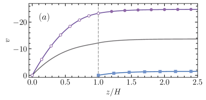
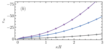
Figure 7: (a) Electroosmotic velocity profiles computed using $\kappa H=3$, $\rho=5$, and $\mathcal{K}H=0$, $1.5$, and $\infty$ (solid curves from top to bottom). Filled and open symbols indicate calculations from Eqs. (17) and Eq. (19). Squares are obtained using $v_{s}=0$, circles correspond to $v_{s}=\psi_{s}+v_{\infty}$, where $v_{\infty}$ is given by Eq. (20); (b) Computed upper bounds ($\mathcal{K}H\to 0$) on $v_{\infty}$ vs. $\kappa H$ (solid curves). From top to bottom $\rho=20,10,$ and $2$. Circles show results of calculations from Eq.(20).

If we suppose $\mathcal{K}H\to\infty$, the slip velocity nearly vanishes, $\psi_{s}\simeq\zeta$, and $v_{\infty}\simeq-\psi_{s}$, which is equivalent to the Smoluchowsky result. Fig. 7(a) includes typical numerical and theoretical $v$-profiles calculated for this case using $\kappa H=3$ and $\rho=5$ that leads to $\psi_{s}\simeq 1.5$. When $\mathcal{K}H\to 0$, integrating Eq.(16) twice, and imposing the continuity of $v$ and $v^{\prime}$ at $z=H$, we find

$$v_{i}\simeq(\psi_{i}-\psi_{0})-\rho\kappa^{2}\left(Hz-\frac{z^{2}}{2}\right),$$ (19)

where for films of any thickness $\psi_{0}$ is given by Eq. (6). The first term reflects the reduction of the potential in the porous coating. The second term is associated with a body force $\rho\kappa^{2}$ that drives the inner flow by acting on the accumulated mobile ions. This contribution resembles the usual no-slip parabolic Poiseuille flow. It follows from Eq.(19) that $-v_{s}\simeq\psi_{0}-\psi_{s}+\dfrac{\rho(\kappa H)^{2}}{2}$. Since $\psi_{0}-\psi_{s}\leq 1$, the second term should dominate even at moderate $\rho$.

The outer velocity $v_{o}$ is given by Eqs.(17) with

$$v_{\infty}\simeq-\left(\psi_{0}+\dfrac{\rho(\kappa H)^{2}}{2}\right)\simeq-\zeta$$ (20)

The $v$-profile for this case is also shown in Fig. 7(a). It turns out that even at moderate $\rho$ and $\kappa H$ one can induce significantly enhanced $v_{\infty}$, which is associated with the emergence of a large slip velocity, $v_{s}$. Also included in Fig. 7(a) is the curve computed using $\mathcal{K}H=1.5$, which is located between two limiting cases and demonstrates quite large $v_{s}$.

We now verify Eq.(20) and plot theoretical $v_{\infty}$ vs. $\kappa H$ in Fig. 7(b) together with numerical data. Upon increasing $\kappa H$ at fixed $\rho$ the amplitude of $v_{\infty}$ grows nonlinearly, and in the case of $\rho\gg 1$ becomes several tens of times faster compared to a no-slip case, even at moderate $\kappa H$. It is tempting to speculate that one can further amplify $v_{\infty}$ making porous film thicker. However, when the film becomes thick enough, the condition $\mathcal{K}H\to 0$ violates, and Eq.(20) is no longer valid.

This implies that mobile ions absorbed within the porous layer actively participate in the flow-driving mechanism by reacting to the field. The porous film acts as a charged immobile surface layer with absorbed mobile ions of the opposite sign, but note the difference from a known example of mobile surface charges at slippery wall Maduar et al. (2015). In the latter case, slippage is of a hydrodynamic origin and mobile surface charges induce a backward flow, reducing the amplification of electro-osmotic flow caused by hydrodynamic slip. By contrast, in the current work an inner solvent flow induces a forward flow and $v_{s}$ itself. However, similarly to hydrophobic electrokinetics Joly et al. (2004); Maduar et al. (2015), our large $\zeta$ no longer reflects the sole $\psi_{s}$. Finally, we would like to stress that a massive amplification of electro-osmotic flow that can be achieved near porous surfaces is of the same order of that at charged super-hydrophobic surfaces Belyaev and Vinogradova (2011), and such a fast flow is in agreement with recent observations Feldmann et al. (2020).

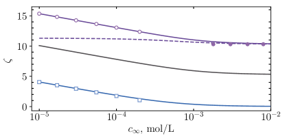
Figure 8: $\zeta$ as a function of $c_{\infty}$ computed for a film of $H=50$ nm, $\varrho=150$ kC/m³, using $\mathcal{K}H=0$, $1.5$, and $\infty$ (solid curves from top to bottom). Dashed curve shows $|v_{s}|$ at $\mathcal{K}H=0$. Squares, open and filled circles plot results of calculations from Eqs.(21), (22), and (23).

So far we have considered the potentials and electro-osmotic velocity at fixed dimensionless $\rho$ and $\kappa H$. Additional insight into the problem can be gleaned by calculating an upper bound on $\zeta$ as a function of $c_{\infty}\propto\kappa^{2}$ at fixed $H$ and $\varrho$. Let us now keep fixed $H=50$ nm and $\varrho=150$ kC/m³, usually referred to as ‘moderate’ Duval et al. (2009), and vary $c_{\infty}$ from $10^{-5}$ to $10^{-2}$ mol/L. Upon increasing $c_{\infty}$ in this range, $\kappa H$ is increased from about 0.5 to 16, and $\rho$ is reduced from about 78 down to 0.1. Therefore, for a given film the required regimes (of thin and thick films, or highly and weakly charged coatings) can be tuned simply by adjusting the concentration of salt.

The bounds on $\zeta$ are shown by lower and upper curves in Fig. 8. If $\mathcal{K}H\to\infty$, $\zeta\simeq\psi_{s}$ decays from ca. 5 ($Z\simeq 125$ mV) practically to zero as $c_{\infty}$ increases, leading to a suppression of a flow. In dilute solutions the lower bound is given by

$$\zeta\simeq\ln{\left(\frac{\varrho}{ec_{\infty}}\right)}-1,$$ (21)

which perfectly fits numerical data. When $\mathcal{K}H\to 0$, $\zeta$ becomes much larger. Thus, with our smallest concentration $\zeta\simeq 15$ (or $Z\simeq 375$ mV). In a dilute solution:

$$\zeta\simeq\ln{\left(\frac{\varrho}{ec_{\infty}}\right)}+\dfrac{2\pi\ell_{B}\varrho H^{2}}{e},$$ (22)

where first term is associated with the potential at the wall. Note that such a logarithmic decay fits well the obtained for real porous materials data Feldmann et al. (2020). For concentrated solutions a large, and independent on salt, zeta-potential is observed. The computed slip velocity, also included in Fig. 8, indicates that this occurs when $\zeta\simeq-v_{s}$ and $\psi_{s}\simeq 0$. Thus, a large zeta-potential emerges solely due to a forward electro-osmotic flow inside a porous film. It is easy to show that it is given by

$$\zeta\simeq\dfrac{2\pi\ell_{B}\varrho H^{2}}{e},$$ (23)

that clarifies the status of second term in Eq.(22). This result is relevant for the understanding zeta-potential measurements with ‘hairy’ surfaces, where it remains finite at even high salt concentrations Donath and Pastushenko (1979); Garg et al. (2016). We recall that Eqs.(21) and (22) represent the lower and upper bounds for $\zeta$ attained at limiting values of $\mathcal{K}H$. Any finite $\mathcal{K}H$ would lead to $\zeta$ confined between the above bounds, as seen in Fig. 8, where we use $\mathcal{K}H=1.5$.

IV Conclusion

In summary, our nonlinear analytic model provides considerable insight into the electro-osmotic equilibria and flows in the presence of porous coatings. It describes absorption capacity of porous films, which is, in turn, responsible for an enhanced electro-osmotic flow. The bounds on zeta-potential we have derived can guide the design of coatings to amplify electrokinetic phenomena.