Use of Cross-validation Bayes Factors to Test Equality of Two Densities

Abstract

We propose a non-parametric, two-sample Bayesian test for checking whether or not two data sets share a common distribution. The test makes use of data splitting ideas and does not require priors for high-dimensional parameter vectors as do other nonparametric Bayesian procedures. We provide evidence that the new procedure provides more stable Bayes factors than do methods based on Pólya trees. Somewhat surprisingly, the behavior of the proposed Bayes factors when the two distributions are the same is usually superior to that of Pólya tree Bayes factors. We showcase the effectiveness of the test by proving its consistency, conducting a simulation study and applying the test to Higgs boson data.

Key words. Bayes factors; Cross-validation; Kernel density estimates; Laplace approximation; Pólya trees; Testing equality of distributions.

1 Introduction

In frequentist hypothesis testing, there is no universal statistic whose values are interpretable across different problems. In contrast, Bayes factors do have a universal interpretation. When the prior probabilities of two hypotheses are the same, the Bayes factor is the ratio of posterior probabilities of the two hypotheses. This is a compelling motivation for developing objective Bayesian procedures that depend only minimally on prior distributions. Hart and Choi (2017) proposed the use of cross-validation Bayes factors (CVBFs) to compare the fit of parametric and nonparametric models. The CVBF is an objective Bayesian procedure in which the nonparametric model is a kernel density estimate, the simplest version of which cannot typically be used in a Bayesian analysis since it only becomes a model once it is computed from data. This problem is sidestepped by computing a kernel estimate from a subset of the data, and then using the estimate as a model for the remainder of the data. As detailed by Hart and Malloure (2019), the notion of a CVBF is also useful in a purely parametric context, wherein data splitting allows one to compare two parametric models via a legitimate Bayes factor that does not require a prior distribution for either model.

The purpose of the current paper is to explore CVBFs in the problem of comparing densities corresponding to two different populations. Given independent random samples $X_{1},\ldots,X_{m}$ and $Y_{1},\ldots,Y_{n}$ from densities $f$ and $g$, respectively, we wish to test the null hypothesis that $f$ and $g$ are identical against the alternative that they are different, without specifying a parametric model for either density. This is accomplished by means of a Bayes factor that makes use of data splitting and kernel density estimates. Unlike the setting of either Hart and Choi (2017) or Hart and Malloure (2019), both hypotheses in the current setting are nonparametric, which necessitates different techniques to show that CVBFs behave desirably. In particular, it is of interest to prove that a CVBF is Bayes consistent when either $f\equiv g$ or the two densities are different. Although the current investigation is restricted to comparison of two densities, we will lay the groundwork for justifying the use of CVBFs in other settings where both hypotheses are nonparametric.

A classic Bayesian approach for checking the equality of two densities involves the construction of priors on the elements of a wide class of distributions. For testing goodness of fit and obtaining posterior predictive distributions, Hanson (2006) proposes methodology based on a Pólya tree prior constructed from a centering distribution. Methods that use a similar strategy for checking equality of two densities have been suggested by Wong et al. (2010), Chen and Hanson (2014) and Holmes et al. (2015). Dunson and Peddada (2008) propose the use of restricted dependent Dirichlet process priors when testing the equality of distributions against ordered alternatives. Both Holmes et al. (2015) and Chen and Hanson (2014) use their Bayes factors in frequentist fashion, i.e., they choose rejection regions to produce desired type I error probabilities. In our opinion, such an approach is not truly Bayesian. If one uses a traditional level of significance such as 0.05, this practice yields a test with the unsettling property that in some cases the hypothesis of equal densities is rejected when the Bayes factor favors equal densities. We prefer an approach that chooses the hypothesis of unequal densities only when the odds in favor of unequal densities has increased in light of the data.

In Section 4 it will be seen that any two-sample procedure based on Bayes factors ultimately depends on the difference between entropy estimates. Beirlant et al. (1997) have suggested using either a kernel density estimate or histogram to estimate entropy and provide conditions under which these types of estimators are consistent. In addition, Beirlant et al. (1997) use entropy estimates to check equality of distributions. Entropy estimates are also seen in the information gain filter in machine learning methods for picking important features; see Sarkar and Goswami (2013). The current paper makes use of results in Hall (1987), who proves consistency of entropy estimates that rely on data-driven smoothing parameters.

An important issue is that of Bayes factor consistency, which we address in Section 4. Suppose the Bayes factor is defined so that values smaller than 1 favor the hypothesis of equal densities. Then consistency means that the Bayes factor converges in probability to $0$ when the densities are equal and diverges to $\infty$ when the densities are unequal. Holmes et al. (2015) contains a proof showing that their Bayes factor is consistent. We argue that our cross-validation Bayes factor is consistent as well. Moreover, when the densities are equal, we argue that a cross-validation Bayes factor converges to $0$ at a much faster rate than do Bayes factors based on traditional Bayesian methods.

A main motivation for our proposed methodology is its conceptual simplicity. The models used are kernel density estimates from training data and each one depends on but a single parameter, a bandwidth. In contrast, the approaches of Hanson (2006) and Holmes et al. (2015) depend on choice of base distribution and $2^{k}$ parameters, where $k$ is typically at least 10. One also needs to choose a prior for all these parameters, although Holmes et al. (2015) propose one that requires specification of just one parameter. In simulations in Section 6 we will compare our method with that of Holmes et al. (2015), and show that the odds ratios produced by the latter test can be highly sensitive to the choice of base distribution.

The rest of the paper may be outlined as follows. In Section 2 we describe in detail our methodology for the two-sample problem. Section 3.1 considers the choice of kernel and also the prior used for the bandwidth parameter, and Section 3.2 investigates the use of a Laplace approximation for marginal likelihoods. In Section 4 we provide theoretical evidence that our Bayes factor is consistent, and in Section 5 we discuss methods for choosing the training set sizes. Finally, Sections 7 and 8 are devoted to a simulation study and real-data analysis, respectively.

2 Methodology

Suppose that we observe independent random samples $X_{1},\ldots,X_{m}$ and $Y_{1},\ldots,Y_{n}$ from cumulative distribution functions $F$ and $G$, respectively. We assume that $F$ and $G$ have respective densities $f$ and $g$, and the goal is to test the following hypotheses by means of a Bayesian approach:

$$H_{0}:\,f\equiv g\quad{\rm vs.}\quad H_{a}:\,f\not\equiv g.$$

We wish to use kernel density estimates to do the testing, and in order to do so we will use the CVBF idea. In contrast to the setting of Hart and Choi (2017), both the null and alternative hypotheses are nonparametric, and hence training data will be used to formulate the alternative and null models. The Bayes factor will then be computed from validation data.

We first introduce some notation. For an arbitrary collection of (scalar) observations $\mbox{\boldmath$Z$}=(Z_{1},\ldots,Z_{n})$, define the kernel density estimate (KDE) $\hat{f}(\,\cdot\,|h,\mbox{\boldmath$Z$})$ by

$$\hat{f}(x|h,\mbox{\boldmath$Z$})=\frac{1}{nh}\sum_{i=1}^{n}K\left(\frac{x-Z_{i}}{h}\right),$$

where the kernel $K$ is a probability density and $h>0$ is the bandwidth. For the moment, all we ask of $K$ is that it be symmetric about 0, unimodal and have finite variance.

Now, partition $X_{1},\ldots,X_{m}$ into $\mbox{\boldmath$X$}_{T}=(X_{1},\ldots,X_{r})$ and $\mbox{\boldmath$X$}_{V}=(X_{r+1},\ldots,X_{m})$, and likewise $Y_{1},\ldots,Y_{n}$ into $\mbox{\boldmath$Y$}_{T}=(Y_{1},\ldots,Y_{s})$ and $\mbox{\boldmath$Y$}_{V}=(Y_{s+1},\ldots,Y_{n})$. Under $H_{0}$ there is a common density, call it $f$. The model for $f$ will be $M_{0}=\{\hat{f}(\,\cdot\,|h,\mbox{\boldmath$X$}_{T},\mbox{\boldmath$Y$}_{T}):h>0\}$. In other words, we pool the two training sets together and use these data to estimate the common density $f$. Under the alternative we have separate models for $f$ and $g$, which are $M_{X}=\{\hat{f}(\,\cdot\,|\alpha,\mbox{\boldmath$X$}_{T}):\alpha>0\}$ and $M_{Y}=\{\hat{f}(\,\cdot\,|\beta,\mbox{\boldmath$Y$}_{T}):\beta>0\}$.

Let $\pi$, $\pi_{X}$ and $\pi_{Y}$ be priors for $h$, $\alpha$ and $\beta$, respectively. The likelihood under $H_{0}$ is

$$L_{0}(h)=\prod_{i=r+1}^{m}\hat{f}(X_{i}|h,\mbox{\boldmath$X$}_{T},\mbox{\boldmath$Y$}_{T})\prod_{j=s+1}^{n}\hat{f}(Y_{j}|h,\mbox{\boldmath$X$}_{T},\mbox{\boldmath$Y$}_{T}).$$

The likelihood under $H_{a}$ is

$$L_{a}(\alpha,\beta)=\prod_{i=r+1}^{m}\hat{f}(X_{i}|\alpha,\mbox{\boldmath$X$}_{T})\prod_{j=s+1}^{n}\hat{f}(Y_{j}|\beta,\mbox{\boldmath$Y$}_{T})=L_{X}(\alpha)L_{Y}(\beta),$$

and the cross-validation Bayes factor (CVBF) is

$$CVBF = \frac{\int_{0}^{\infty}\int_{0}^{\infty}\pi_{X}(\alpha)\pi_{Y}(\beta)L_{a}(\alpha,\beta)\,d\alpha d\beta}{\int_{0}^{\infty}\pi(h)L_{0}(h)\,dh}$$ (1)

$$= \frac{\int_{0}^{\infty}\pi_{X}(\alpha)L_{X}(\alpha)\,d\alpha\cdot\int_{0}^{\infty}\pi_{Y}(\beta)L_{Y}(\beta)\,d\beta}{\int_{0}^{\infty}\pi(h)L_{0}(h)\,dh}.$$

Interestingly, each of $M_{0}$, $M_{X}$ and $M_{Y}$ is a parametric model, inasmuch as each depends on just a single parameter, a bandwidth. It should be acknowledged that we know with certainty that, for example, $M_{X}$ does not contain the true density $f$. However, there is a key difference between $M_{X}$ and a traditional one-parameter model. Since KDEs are consistent estimators, we have reason to believe that some members of $M_{X}$ will be quite close to $f$, especially if the training set size $r$ is large. In contrast, members of a traditional one-parameter model, such as all $N(\mu,1)$ densities, would be close to the truth only under very special circumstances. So, in spite of being formally “wrong,” $M_{X}$ can be expected to be a good model, which echoes the sentiment of George Box in his famous quote about statistical models.

Even if one objects to our models not formally containing the truth, the same criticism can arguably be leveled against the Pólya tree approach of Holmes et al. (2015). Each element of the parameter space in that approach is of histogram type, and since one usually envisions a certain degree of smoothness in the underlying density, the true density does not necessarily lie in the parameter space employed by Pólya trees.

We close this section with some remarks about our methodology.

• The quantity (1) is referred to as a cross-validation Bayes factor (Hart and Choi, 2017) since each data set is split into two parts. For example, the data $X_{1},\ldots,X_{m}$ are split into a training set, $\mbox{\boldmath$X$}_{T}$, and a validation set, $\mbox{\boldmath$X$}_{V}$.

• In spite of the fact that the models being compared in $CVBF$ are formulated from data, it is important to appreciate that $CVBF$ is a legitimate Bayes factor. This is because the models are defined from data that are independent of the validation sets $\mbox{\boldmath$X$}_{V}$ and $\mbox{\boldmath$Y$}_{V}$. The Bayesian paradigm does not specify where posited models must come from, so long as they are not defined from the data used to evaluate those models.

• By assuming that the bandwidths $\alpha$ and $\beta$ are a priori independent, the computation of $CVBF$ reduces to calculating three separate marginals, each of which has the form dealt with in Hart and Choi (2017).

• Györfi et al. (1985) show that the $L_{1}$ norm difference between a kernel density estimate and the true density tends to 0 for any kernel integrating to 1 as long as the sample size $n$ tends to $\infty$, the bandwidth $h$ tends to 0, and $nh\rightarrow\infty$. Because of results like this, the conventional wisdom in kernel density estimation is that the choice of kernel $K$ is not overly important. This is not at all the case in the current context. In Section 3.1 we will point out the importance of using relatively heavy-tailed kernels, a specific version of which is proposed.

• Ideally a CVBF should not depend on the particular data split that is used. Therefore, we suggest that one use the geometric mean of $CVBF$ values calculated from a number of different randomly chosen splits.

3 Implementation issues

Some practical issues must be addressed in order to make use of CVBFs. A kernel has to be chosen for each of the KDEs, and priors for the bandwidths of the KDEs are needed. Furthermore, the integrals defining the three marginals cannot (in general) be computed analytically, and hence approximations of the integrals are necessary. We first address the choice of kernel and priors.

3.1 Choice of kernel and priors

For densities $f_{1}$ and $f_{2}$, the Kullback-Leibler divergence between $f_{1}$ and $f_{2}$ is defined to be

$$KL(f_{1},f_{2})=\int_{-\infty}^{\infty}f_{1}(x)\log\left(\frac{f_{1}(x)}{f_{2}(x)}\right)\,dx.$$

As will be discussed in Section 4, consistency of our proposed Bayes factor depends crucially on the behavior of $KL(f,\hat{f}(\,\cdot\,|\alpha,\mbox{\boldmath$X$}_{T}))$ and $KL(g,\hat{f}(\,\cdot\,|\beta,\mbox{\boldmath$Y$}_{T}))$. Hall (1987) shows that the right sort of kernel needs to be used to ensure that these divergences are well-behaved. A number of practical and technical difficulties arising from tail behavior of the underlying density are eliminated if one uses a relatively heavy-tailed kernel. A kernel that suffices in this regard is the following that was proposed by Hall (1987):

$$K_{0}(z)=\frac{1}{\sqrt{8\pi e}\,\Phi(1)}\exp\left[-\frac{1}{2}(\log(1+|z|))^{2}\right],$$ (2)

where $\Phi$ is the standard normal distribution function.

Hall (1987) provides an example of when the popular Gaussian kernel can fail in our context. Suppose that $f$ is a Cauchy density, and one estimates $f$ by a kernel estimator $\hat{f}_{h}$ with Gaussian kernel and bandwidth $h$. Then (i) the expected Kullback-Leibler loss of $\hat{f}_{h}$ is infinite and (ii) the likelihood cross-validation choice of $h$ diverges to infinity. In contrast, if kernel $K_{0}$ is used in this case, then the likelihood cross-validation bandwidth is asymptotic to the minimizer of expected Kullback-Leibler loss. Simulations in Section 6 show that these results for the Cauchy distribution appear to be true for the version of cross-validation used in the current paper.

If one is confident that the tails of the underlying density are no heavier than those of a Gaussian density, then it would be appropriate to use a Gaussian kernel in our procedure. Simulations we have done suggest that the Gaussian kernel produces somewhat more stable Bayes factors than does $K_{0}$ in the case of light-tailed densities. However, when there is uncertainty about the tails of the underlying density, $K_{0}$ is a much better choice for the kernel. For this reason we will use $K_{0}$ for all simulations and data analyses in this paper.

The prior we propose for each bandwidth is as follows, which is the same type as used by Hart and Choi (2017):

$$\pi(h|\gamma)=\frac{2\gamma}{\sqrt{\pi}h^{2}}\exp\left(-\frac{\gamma^{2}}{h^{2}}\right)I_{(0,\infty)}(h).$$ (3)

An aspect of this prior that we find appealing is that it tends to $0$ as $h$ tends to 0. This in concert with the fact that, due to the data-driven nature of our kernel density estimation models, we are (essentially) a priori certain that the very smallest bandwidths produce untenable densities.

The mode of (3) is $\gamma$, and we propose that for each marginal, $\gamma$ be chosen to equal the maximizer of the corresponding likelihood. For example, for the marginal $\int_{0}^{\infty}\pi_{X}(\alpha)L_{X}(\alpha)\,d\alpha$, we take $\pi_{X}\equiv\pi(\,\cdot\,|\hat{\gamma})$, where $\hat{\gamma}$ is the maximizer of $L_{X}$. The scale of $\pi(\,\cdot\,|\gamma)$ is proportional to $\gamma$, which entails that the prior $\pi(\,\cdot\,|\hat{\gamma})$ has low information relative to the likelihood. This is because the variance of the cross-validation bandwidth $\hat{\gamma}$ is $o(\hat{\gamma})$, a fact that is ensured by using the kernel $K_{0}$. Centering a low information prior at the maximizer of the likelihood is akin to using a unit reference prior (Consonni et al., 2018) centered at the data, which by now is a fairly common practice.

3.2 Laplace approximation

Interestingly, there exists a closed-form expression for each marginal if one uses a Gaussian kernel in conjunction with a prior of the form (3). This results from the fact that, for example, $\pi(\alpha|\gamma)L_{X}(\alpha)$ is a linear combination of functions each of which is proportional to a function of the form $\alpha^{k}\exp(-A/\alpha^{2})$, whose integral over $(0,\infty)$ may be expressed in terms of the gamma function. The practical usefulness of this closed-form solution is limited for two reasons. First, as was noted in Section 3.1, the Gaussian kernel is not a good all-purpose kernel, and secondly it turns out that more computations are required for the closed form solution than for standard methods of approximating integrals. The solution requires $r^{m-r}$ sums to be computed, where $r$ is the size of the training set and $m-r$ the size of the validation set. For these reasons we will not pursue the closed form solution further.

In general, the integrations required to calculate a $CVBF$ cannot be done analytically. Hart and Choi (2017) used numerical integration to approximate marginal likelihoods, either by simple or adaptive quadrature. Other methods that could be used are importance sampling, bridge sampling or a Laplace approximation. A Laplace approximation has the advantage of being less computationally intensive. Let $\hat{h}$ be the maximizer of $L_{0}$ and define

$$\hat{H}=-\frac{\partial^{2}}{\partial h^{2}}\log L_{0}(h)\Big{|}_{h=\hat{h}}.$$

Then the Laplace approximation of $\int\pi(h)L_{0}(h)\,dh$ is

$$\int\pi(h)L_{0}(h)\,dh\approx\sqrt{\frac{2\pi}{\hat{H}}}\cdot\pi(\hat{h})L_{0}(\hat{h}).$$

The quantity $\hat{H}$ can be expressed as a functional of kernel estimates based on the kernel $K$ and two other related kernels. An expression for $\hat{H}$ may be found in the Appendix.

To investigate how well the Laplace approximation works in our context we generate samples from a standard normal distribution and compare the Laplace approximation of the marginal likelihood with an approximation using the R function integrate (which uses adaptive quadrature). Data were generated from a standard normal distribution and sample sizes 200, 500 and 1000 were considered. The kernel used was $K_{0}$, and the prior was (3) with $\gamma$ taken to be the maximizer of the likelihood. The training set size was always 1/4 of the sample size, and 500 replications for each $n$ were considered. Table 1 summarizes the results.

$n$	Median	Interquartile range
200	$6.99\cdot 10^{-4}$	$3.46\cdot 10^{-4}$
500	$2.66\cdot 10^{-4}$	$1.80\cdot 10^{-4}$
1000	$1.33\cdot 10^{-4}$	$2.77\cdot 10^{-4}$

Table 1: Relative error of Laplace approximation of marginal likelihood. Each median and interquartile range is based on 500 replications. The measure of error is $|(log\hat{M}-\log M)/\log M|$, where $M$ and $\hat{M}$ are quadrature and Laplace approximations, respectively, of the marginal.

The Laplace approximations were excellent, with the median relative error being no larger than 0.000699 and becoming smaller as the sample size increased. A plot of the results for $n=500$ is given in Figure 1. We also found that the computations for our Laplace approximation are 7 to 8 times faster at $n=1000$ than those for the quadrature approximation when running on an 8 core Intel Skylake 6132 CPU running at 2.6GHz with 32GB of 2666MHz DDR4 memory. For these reasons we will use the Laplace approximation in all subsequent simulations and examples.

We note that the parameter of our prior is chosen so that the prior mode is equal to the maximizer of the likelihood. This has two computational benefits. First of all, our algorithm starts by determining the maximizer of the log-likelihood, which is necessary to avoid underflow problems. But once this maximizer has been determined it is not necessary to find the posterior mode since the two quantities are one and the same. Secondly, choosing the prior parameter in this way renders null the distinction between the two versions of the Laplace approximation, one using the maximizer of $L_{0}$ and the other the maximizer of $\pi L_{0}$.

Figure 1: Laplace and quadrature approximations to log-marginal likelihoods. These results are for the case where the training set and validation sizes were $125$ and $375$, respectively.

4 Bayes consistency

Here we address the consistency of a $CVBF$ in the two-sample problem. We begin with a list of assumptions.

• The Laplace approximation of each of the three marginals is asymptotically correct in that the log of the marginal likelihood is equal to the log of the Laplace approximation plus a term that is negligible in probability relative to the approximation.

• The densities $f$ and $g$ are bounded away from 0 and $\infty$ on $(-\lambda,\lambda)$ for each $\lambda>0$, with $f(x)\sim c_{1}x^{-a_{1}}$ and $f(-x)\sim c_{2}x^{-a_{2}}$ as $x\rightarrow\infty$, where both $c_{1}$ and $c_{2}$ are positive and $a_{1}$ and $a_{2}$ larger than $1$. Density $g$ satisfies the same properties as $f$, albeit with possibly different constants.

• The second derivatives $f^{\prime\prime}$ and $g^{\prime\prime}$ exist and are bounded and almost everywhere continuous on $(-\infty,\infty)$. In addition, for a constant $C_{2}<\infty$,

  $$|f^{\prime\prime}(x)|\leq C_{2}x^{-a_{1}-2}\quad{\rm and}\quad|f^{\prime\prime}(-x)|\leq C_{2}x^{-a_{2}-2}\quad{\rm for}\ x>1,$$

  where $a_{1}$ and $a_{2}$ are the same as in A2. The function $g^{\prime\prime}$ satisfies the same properties as $f^{\prime\prime}$ with possibly different constants.

• The kernel used is $K_{0}$, as defined in (2).

Conditions A2 and A3 are those of Hall (1987) and are needed to ensure that the maximizer of the likelihood cross-validation criterion is optimal in a Kullback-Leibler sense. Hall (1987) provides another set of conditions that could be used in place of A2 and A3. These conditions deal with compactly supported densities, but for the sake of brevity we do not repeat these. Furthermore, the kernel conditions of Hall (1987) are satisfied by kernels other than $K_{0}$, but notably the Gaussian kernel does not satisfy his conditions.

We wish to argue that the statistic $CVBF$ defined by (1) is Bayes consistent under both null and alternative hypotheses. Initially, we will consider the null case, i.e., $f\equiv g$. Each Laplace approximation depends on a term $\widehat{H}$ for which $\log\widehat{H}=O_{p}(\log n)$. Define

$$\widehat{BF}=\frac{\pi_{X}(\hat{\alpha})L_{X}(\hat{\alpha})\pi_{Y}(\hat{\beta})L_{Y}(\hat{\beta})}{\pi(\hat{h})L_{0}(\hat{h})},$$

where $\hat{\alpha}$, $\hat{\beta}$ and $\hat{h}$ are the maximizers of $L_{X}$, $L_{Y}$ and $L_{0}$, respectively. We will see that $\log n$ is of smaller order than $\log\widehat{BF}$ under both hypotheses, and therefore by A1 it is sufficient to consider $\widehat{BF}$ when investigating consistency.

Although probably not necessary, we assume at this point that $m-r>r$ and $n-s>s$. An important aspect of $\widehat{BF}$ is the behavior of the maximizers of the likelihoods. Consider, for example, $\hat{\alpha}$. We claim that under general conditions $\hat{\alpha}$ is asymptotic in probability to the minimizer, $\alpha_{r}$, of $E[KL(f,\hat{f}(\,\cdot\,|\alpha,\mbox{\boldmath$X$}_{T}))]$ as $r$ and $m-r$ tend to $\infty$. Hall (1987) proved precisely this result assuming that the KDE uses kernel (2) and its bandwidth is chosen by leave-one-out likelihood cross-validation. This version of cross-validation chooses the bandwidth of $\hat{f}(\,\cdot\,|\alpha,\mbox{\boldmath$X$}_{T})$ to maximize, with respect to $\alpha$,

$$\ell(\alpha)=\prod_{i=1}^{r}\hat{f}(X_{i}|\alpha,\mbox{\boldmath$X$}_{T}^{i}),$$ (4)

where $\mbox{\boldmath$X$}_{T}^{i}$ is all the training data except for $X_{i}$, $i=1,\ldots,r$. Using essentially the same proof as in Hall (1987), it can be shown that our version of likelihood cross-validation is at least as efficient as the leave-one-out version. Intuitively, this is plausible since our version of the cross-validation curve is

$$L(\alpha)=\prod_{i=r+1}^{m}\hat{f}(X_{i}|\alpha,\mbox{\boldmath$X$}_{T}).$$ (5)

In comparison to (4), (5) has two advantages: $m-r>r$ and the validation data $X_{r+1},\ldots,X_{m}$ are completely independent of $\hat{f}(\,\cdot\,|\alpha,\mbox{\boldmath$X$}_{T})$. It is also worth noting that van der Laan et al. (2004) prove optimality of the version of likelihood cross-validation that we use, albeit under more restrictive conditions than those of Hall (1987).

Now, let $\beta_{s}$ and $h_{r+s}$ denote the minimizers of $E[KL(f,\hat{f}(\,\cdot\,|\beta,\mbox{\boldmath$Y$}_{T}))]$ and $E[KL(f,\hat{f}(\,\cdot\,|$ $h,\mbox{\boldmath$X$}_{T},\mbox{\boldmath$Y$}_{T}))]$, respectively. Then the optimality of likelihood cross-validation implies that the difference between $\log\widehat{BF}$ and $\log\widetilde{BF}$ is negligible, where

$$\widetilde{BF}=\frac{\pi_{X}(\alpha_{r})L_{X}(\alpha_{r})\pi_{Y}(\beta_{s})L_{Y}(\beta_{s})}{\pi(h_{r+s})L_{0}(h_{r+s})}.$$

If the priors and their parameters are chosen as discussed in Section 3.1, then, for example,

$$\log\pi_{X}(\alpha_{r}) = \log(2/\sqrt{\pi})+\log(\hat{\alpha}/\alpha_{r}^{2})-(\hat{\alpha}/\alpha_{r})^{2}$$

$$= \log(2/\sqrt{\pi})-\log(\alpha_{r})-1+o_{p}(1)$$

$$= O_{p}(\log m),$$

with the last equality owing to the fact that the optimal bandwidth $\alpha_{r}$ is of order $r^{-a}$ for $0<a<1$. Similar results are true for the other two terms depending on priors. This entails that the effect of the priors on $\log\widetilde{BF}$ is negligible compared to the contribution from the likelihoods, as we will see subsequently.

Defining $\hat{f}_{X}\equiv\hat{f}(\,\cdot\,|\alpha_{r},\mbox{\boldmath$X$}_{T})$, $\hat{f}_{Y}\equiv\hat{f}(\,\cdot\,|\beta_{s},\mbox{\boldmath$Y$}_{T})$, $\hat{f}_{X,Y}\equiv\hat{f}(\,\cdot\,|h_{r+s},\mbox{\boldmath$X$}_{T},\mbox{\boldmath$Y$}_{T})$ and $LR=L_{X}(\alpha_{r})L_{Y}(\beta_{s})/L_{0}(h_{r+s})$, we have

$$\log(LR)=(m-r)\int\log\left(\frac{\hat{f}_{X}(x)}{\hat{f}_{X,Y}(x)}\right)dF_{m-r}(x)+(n-s)\int\log\left(\frac{\hat{f}_{Y}(y)}{\hat{f}_{X,Y}(y)}\right)dG_{n-s}(y),$$ (6)

where $F_{m-r}$ and $G_{n-s}$ are the empirical cdfs of $\mbox{\boldmath$X$}_{V}$ and $\mbox{\boldmath$Y$}_{V}$, respectively. Note that $\log(LR)$ depends intimately on entropy estimates of the form $-\sum_{i=1}^{m}\log\hat{f}(X_{i})/m$. From (6) we have

$$\log(LR) = (m-r)\left[KL(f,\hat{f}_{X,Y})-KL(f,\hat{f}_{X})\right]+(n-s)\left[KL(f,\hat{f}_{X,Y})-KL(f,\hat{f}_{Y})\right]$$ (7)

$$+\delta_{1}+\delta_{2},$$

where

$$\delta_{1}=(m-r)\left\{\int\log\left(\frac{\hat{f}_{X}(x)}{\hat{f}_{X,Y}(x)}\right)\left[dF_{m-r}(x)-dF(x)\right]\right\}$$

and

$$\delta_{2}=(n-s)\left\{\int\log\left(\frac{\hat{f}_{Y}(y)}{\hat{f}_{X,Y}(y)}\right)\left[dG_{n-s}(y)-dF(x)\right]\right\}.$$

Under the conditions of Hall (1987), the quantity $\delta_{1}+\delta_{2}$ is negligible relative to the other terms in $\log(LR)$, and

$$KL(f,\hat{f}_{X})=C_{f}r^{-a}+o_{p}(r^{-a}),$$ (8)

where $C_{f}$ is a positive constant depending on $f$ (and $K$) and $a$ is a constant such that $0<a<4/5$. The other two Kullback-Leibler discrepancies admit similar expansions, differing only with respect to sample size. Expansion (8) and the argument above imply that

$$\log(LR) = C_{f}\left\{(m-r)\left[\frac{1}{(r+s)^{a}}-\frac{1}{r^{a}}\right]+(n-s)\left[\frac{1}{(r+s)^{a}}-\frac{1}{s^{a}}\right]\right\}$$

$$+o_{p}\left(\frac{(m-r)}{r^{a}}+\frac{(n-s)}{s^{a}}\right).$$

Obviously, each of the two terms in square brackets is negative, as desired in the present case where the two densities are the same. Furthermore, if $r$ and $s$ tend to $\infty$ in such a way that $r/(r+s)$ converges to $q$ for $0<q<1$, then

$$\log(LR)\sim C_{f}\left\{\frac{(m-r)}{r^{a}}\cdot(q^{a}-1)+\frac{(n-s)}{s^{a}}\cdot((1-q)^{a}-1)\right\}.$$ (9)

Suppose that $r<mp$ and $s<np$ for $0<p<1$. Then since $a<4/5$, the last quantity will tend to $-\infty$ as $m$, $n$, $r$ and $s$ tend to $\infty$.

We turn now to the case where the alternative is true. To fix ideas, we define $f$ and $g$ to be different if and only if $\int|f-g|>0$. For $0<\lambda<1$, $f$ and $g$ different implies that $\int|f-(\lambda f+(1-\lambda)g|>0$ and $\int|g-(\lambda f+(1-\lambda)g|>0$, inequalities that are necesssary for our consistency argument. Our new argument is essentially the same as in the null case until we arrive at (7), which now becomes

$$\log(LR) = (m-r)\left[KL(f,\hat{f}_{X,Y})-KL(f,\hat{f}_{X})\right]+(n-s)\left[KL(g,\hat{f}_{X,Y})-KL(g,\hat{f}_{Y})\right]$$ (10)

$$+\delta_{1}+\delta_{2}.$$

The discrepancies $KL(f,\hat{f}_{X})$ and $KL(g,\hat{f}_{Y})$ tend to 0 in probability under the conditions of Hall (1987). If $r/(r+s)$ tends to $q$, $0<q<1$, then $KL(f,\hat{f}_{X,Y})$ and $KL(g,\hat{f}_{XY})$ converge in probability to $KL(f,qf+(1-q)g)$ and $KL(g,qf+(1-q)g)$, respectively. Since each of $\int|f-(qf+(1-q)g)|$ and $\int|f-(qf+(1-q)g)|$ is positive, it follows from Pinsker’s inequality that $KL(f,qf+(1-q)g)$ and $KL(g,qf+(1-q)g)$ are both positive. Therefore, $\log(LR)$ is asympotic to $Am+Bn$ for positive constants $A$ and $B$, and consistency is proven.

We close this section with the following remarks.

• Expression (10), which is correct under both null and alternative hypotheses, shows that the density estimates from the training data have the main responsibility for getting the sign of $\log(LR)$ right.

• When the null is true, we wish $\log(LR)$ to be negative. This occurs with high probability owing to the fact that $KL(f,\hat{f})$ tends to be smaller when the sample size on which $\hat{f}$ is based becomes larger. Therefore, to make it more likely that both $\left[KL(f,\hat{f}_{X,Y})-KL(f,\hat{f}_{X})\right]$ and $\left[KL(f,\hat{f}_{X,Y})-KL(f,\hat{f}_{Y})\right]$ are negative, it stands to reason that $r/(r+s)$ should not be too close to either 0 or 1.

• When the alternative is true, we want $\log(LR)$ to be positive. This is guaranteed if $\hat{f}_{X}$ is closer to $f$ (in the Kullback-Leibler sense) than is $\hat{f}_{X,Y}$, and $\hat{f}_{Y}$ is closer to $g$ than is $\hat{f}_{X,Y}$. To ensure that this is true, one should make $r$ and $s$ as large as possible.

• Assuming that the sign of $\log(LR)$ is correct, the weight of evidence in favor of the alternative is dictated by the sizes of $m-r$ and $n-s$.

• When $n$ and $m$ are sufficiently large, a good way to ensure that both the sign and magnitude of $\log(LR)$ are suitable is to take $r\sim m/2$ and $s\sim n/2$.

• Expression (9) entails that, under the null, $CVBF$ tends to 0 at a much faster rate than is typical for traditional Bayesian tests. Suppose, for example, that $r\sim m/2$ and $s\sim n/2$. Then $\log(LR)\sim-(C_{1}m^{1-a}+C_{2}n^{1-a})$ for positive constants $C_{1}$ and $C_{2}$ and $0<a<4/5$. In contrast, when one uses a nonparametric Bayesian procedure in which the null model is nested within the alternative, the log-Bayes factor typically diverges to $-\infty$ at a rate that is only logarithmic in the sample size; see, for example McVinish et al. (2009).

5 Choice of training set size

We now discuss the choice of training set sizes $r$ and $s$ for given sets of data. Two competing ideas are at play when choosing these quantities. First of all, it is desired that the KDEs from the training data be good representations of $f$ and $g$, a desire that calls for large $r$ and $s$. On the other hand, we would like as much data as possible for computing the Bayes factor, which asks that $m-r$ and $n-s$ be large. To balance these two considerations it seems intuitively reasonable that one choose $r=[m/2]$ and $s=[n/2]$, where $[x]$ denotes the integer closest to but not larger than $x$. Indeed, when $m+n$ is smaller than 5000 or so, these are our suggested default choices of $r$ and $s$. The main reason that $r=[m/2]$ and $s=[n/2]$ are not suggested for very large sample sizes is that they maximize the length of time needed to compute the Bayes factor. To explain why, consider the marginal based on just $X_{1},\ldots,X_{m}$. This marginal requires calculation of $m-r$ kernel estimates, each of which involves $r$ additions. So, a total of $r(m-r)$ operations are required for each likelihood evaluation, and this number is maximized when $r=m/2$. This result is of particular interest for extremely large datasets. In this case it is unlikely that half of the full dataset is required for computing a good training density, and hence significant reductions in computing time can be gained by choosing a training set size that is much smaller than the validation set size.

Aside from computing issues, there is another reason why $r=[m/2]$ and $s=[n/2]$ are not suggested for very large data sets. Doing so is undoubtedly not optimal from the point of view of producing good Bayes factors. Expressions (9) and (10) suggest that the magnitude of log-$CVBF$ tends to decrease with an increase in the training set size, this being true under both null and alternative hypotheses. Arguing on a more intutive level, suppose that $m=n=50,000$. Choosing $r=s=25,000$ is undoubtedly overkill for obtaining reliable KDEs and reduces the number of data available for computing the Bayes factor(s). A whole range of much smaller choices of $r=s$ will produce high quality KDEs and leave more data for computing CVBFs.

Dependence of Bayes procedures on tuning parameters or hyperparameters, especially in nonparametric settings, is not at all unusual. For example, the Pólya tree method of Holmes et al. (2015) relies upon specifying the prior precision parameter $c$. The authors of that article state that values of $c$ between $1$ and $10$ work well in practice, but they also recommend checking the sensitivity of their Bayes factor to choice of $c$. When employing our CVBF methodology the training set sizes may be regarded as tuning parameters, and as with any Bayes procedure it is recommended that one investigate sensitivity of $CVBF$ to different choices for $(r,s)$. If all the Bayes factors computed are in basic agreement, then the decision is clear.

To deal with cases where Bayes factors corresponding to different choices of $(r,s)$ are not in agreement, we propose that one treat $(r,s)$ as a parameter that has a prior distribution. To simplify matters, we assume that $m=n$ and $r=s$. Now, divide each data set into training and validation sets of size $K$ and $m-K$, respectively. For sample sizes that are not extremely large one could take $K=[m/2]$, and otherwise $K$ could be some reasonable upper bound on $r$. Let ${\cal T}$ be some subset of training set sizes between 1 and $K$, and suppose that prior probabilities $p(r)$ are assigned to the elements of ${\cal T}$ in such a way that $\sum_{r\in{\cal T}}p(r)=1$. (A good default choice would be to assume that the training set sizes are equally likely.) For each $r\in{\cal T}$ we randomly select $r$ values (without replacement) from each of the two sets of training data. From these two data sets of size $r$ we determine kernel models $M_{X,r}$, $M_{Y,r}$ and $M_{0r}$, as described in Section 2. From these we may compute marginal likelihoods $m_{0,r}$ and $m_{r}$ corresponding to the null and alternative hypotheses, respectively, from the validation data, again as described in Section 2. Assuming that the prior probability of $H_{0}$ is the same for each training set size, a Bayes factor for comparing the alternative and null models is

$$\frac{\sum_{r\in{\cal T}}p(r)m_{r}}{\sum_{r\in{\cal T}}p(r)m_{0,r}}.$$ (11)

Importantly, this methodology is in strict adherence to Bayesian principles, inasmuch as all models are formulated from training data, and the two hypotheses are assessed from the same set of validation data, which is independent of the training data. This method will be illustrated in our real data example in Section 7.

6 Simulations

Initially we provide evidence that our cross-validation method of selecting a bandwidth is efficient in the sense of Hall (1987). Suppose we have independent random samples $\mbox{\boldmath$X$}_{T}=(X_{1},\ldots,X_{r})$ and $\mbox{\boldmath$X$}_{V}=X_{r+1},\ldots,X_{m}$, each from the same density $f$. We wish to select the bandwidth of the KDE $\hat{f}(\,\cdot\,|h,\mbox{\boldmath$X$}_{T})$. We do so in two ways, by determining the maximizers of the criteria defined in (4) and (5). Table 2 provides results for a setting in which data are drawn from $f\equiv\hbox{standard Cauchy density}$ and the kernel used is the Hall kernel, as defined in (2). One hundred replications of each of two cases were performed: $(r,m-r)=(200,300)$ and $(r,m-r)=(400,600)$. For each data set three bandwidths were determined: the maximizers of (4) and (5) and the minimizer of the Kullback-Leibler discrepancy between KDEs and the true Cauchy density.

$(r,m-r)$	Mean $\hat{h}_{LO}$	SD $\hat{h}_{LO}$	Mean $\hat{h}_{CV}$	SD $\hat{h}_{CV}$	Mean $\hat{h}_{KL}$	SD $\hat{h}_{KL}$
$(200,300)$	0.320	0.080	0.314	0.073	0.313	0.025
$(400,600)$	0.277	0.066	0.265	0.044	0.268	0.020

Table 2: Means and standard deviations of cross-validation bandwidths and Kullback-Leibler optimal bandwidths. The bandwidths $\hat{h}_{LO}$ and $\hat{h}_{CV}$ maximize (4) and (5), respectively, and $\hat{h}_{KL}$ optimizes Kullback-Leibler loss. Results are based on 100 replications for each choice of $(r,m-r)$.

The cross-validation bandwidths behave in accordance with the theory described in Section 4. At a given $(r,m-r)$, the means of $\hat{h}_{LO}$ and $\hat{h}_{CV}$ are approximately equal to the mean of the optimal bandwidths. Furthermore, the standard deviations of the cross-validation bandwidths decrease when $r$ amd $m-r$ increase. Figure 2 illustrates that the bandwidth maximizing (5) tends to be closer to the Kullback-Leibler optimal bandwidth than is the maximizer of leave-one-out cross-validation.

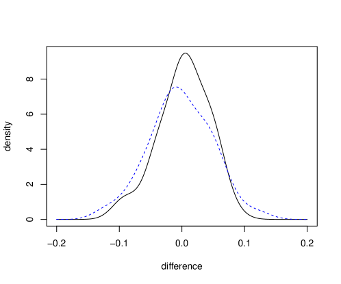
Figure 2: Kernel density estimates of bandwidth differences distributions. The solid line is a KDE of the difference between the Kullback-Leibler optimal bandwidth and the maximizer of (5), while the dashed blue line is a KDE of the difference between the Kullback-Leibler optimal bandwidth and the maximizer of (4). Results are based on 100 replications and the case where $r$ is 400 and $m-r$ is 600.

As noted previously, Hall (1987) proved that when the tails of the underlying density are sufficiently heavy and one uses a Gaussian kernel, then likelihood cross-validation chooses a bandwidth that diverges to infinity as sample size increases without bound. To illustrate this point, we repeated the previous simulation using a Gaussian kernel instead of (2). For each data set, $L(h)$ was maximized over the interval $(0.001,30)$. At $(r,m-r)=(200,300)$, the average value of the cross-validation bandwidths was 13.4, and 16 of the 100 values were 30. At $(r,m-r)=(400,600)$ the average bandwidth was 12.8 and 6 of the 100 were 30. These bandwidths are obviously much too big to provide reasonable estimates of the true density.

We turn now to simulations investigating various aspects of our CVBF methodology. Part of this investigation addresses how our test fares in comparison to the Kolmogorov-Smirnov (KS) test and to the Pólya tree test of Holmes et al. (2015). For each case where the Pólya tree test is run, the precision parameter $c$ is taken to be 1. We do this for two reasons. Primarily, this choice proved to be successful in the study of Holmes et al. (2015). Secondly, choosing $c$ to be closer to 0 seems to have the effect of making the test depend less on the centering distribution utilized and more on the empirical cdf, which is what would be desired in the non-parametric setting (Hanson, 2006).

For the null case, we generate data from a standard normal distribution, taking $m=n$ for sample sizes 200, 400 and 800. For the CVBF training set sizes we took $r=s$, with $r=50$, $75$ and $112$ at sample sizes $200$, $400$, and $800$, respectively. So, the training set size increases by fifty percent when the sample size doubles. The value of CVBF for a given replication was the geometric mean of CVBFs corresponding to 30 pairs of randomly selected training sets, and 1500 replications were performed at each $n$. The kernel $K_{0}$ was used for all our simulations, and the prior for each bandwidth was (3) with $\gamma$ equal to the maximizer of the corresponding likelihood.

The results are shown in Figures 3 and 4. All but two of the 4500 values of $\log(CVBF)$ computed were smaller than 0. At $n=400$, all 1500 replications produced a value of $\log(CVBF)$ that was smaller than 0, and just two values larger than $-\log(20)$, a value considered to be the threshold for “strong” evidence in favor of the null hypothesis (Kass and Raftery, 1995). At $n=800$ all 1500 values of $\log(CVBF)$ were smaller than $-\log(20)$, and at $n=200$ all but 46 values of $\log(CVBF)$ were below this threshold. The near linear decrease in the estimates of $E(\log(CVBF))$ is evidence for the exponential rate of convergence of $CVBF$ that was discussed in Remark R6. The Pólya tree Bayes factors do not behave as well as the CVBFs. For example, at $n=400$, the median $\log(CVBF)$ is $-10.26$, while the median Pólya tree $\log(BF)$ is but $-4.06$. At $n=800$, $5$% of the Pólya tree $\log(BF)$ values are actually larger than 0, while the largest $\log(CVBF)$ is $-7.83$. When a particular model is true, we desire that a Bayes factor provide the strongest possible evidence in favor of that model, and on this score CVBF has outperformed the Pólya tree method in this example.

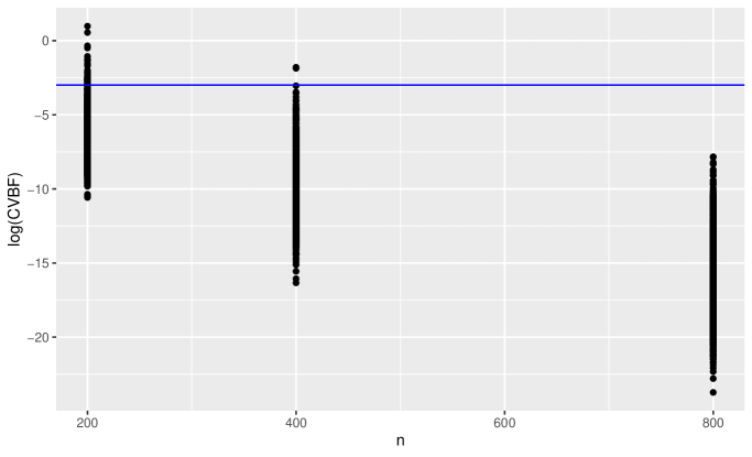
Figure 3: Values of $\log(CVBF)$ when the null hypothesis is true. Each point corresponds to $X$ and $Y$ samples each of size $n$ from a $N(0,1)$ distribution. The standard deviations of the log-Bayes factors are $1.60$, $1.95$ and $2.41$, for $n=200$, $400$, and $800$, respectively.

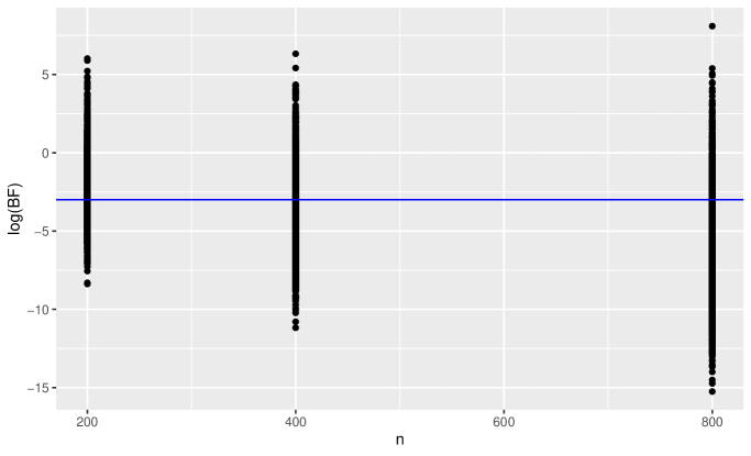
Figure 4: Values of $\log(BF)$ for the Pólya tree when the null hypothesis is true. Each point corresponds to $X$ and $Y$ samples each of size $n$ from a $N(0,1)$ distribution. The standard deviations of the log-Bayes factors are $2.05$, $2.52$ and $3.31$ for $n=200$, $400$, and $800$, respectively.

Under the alternative hypothesis, we use a version of BayesSim, as proposed by Hart (2017), for data generation. Here, the $X$ sample is drawn from a density $f$. To obtain the $Y$ sample, we first draw $p$ from beta$(1/2,1/2)$, a beta distribution with both parameters equal to 1/2, and then the $Y$ sample is drawn from a mixture of the form $(1-p)f(x)+pg(x)$, where $g$ is different from $f$. This approach allows one to infer the behavior of CVBF for mixing proportions $p$ ranging from 0 to 1, where the discrepancy between the $X$ and $Y$ densities increases with $p$. Sample sizes of $m=n=280$ were considered, the training set sizes were selected to be 120, and 500 values of $p$ were selected for each choice of $(f,g)$. For a given replication, thirty random splits for each of $X$ and $Y$ were used. For each pair of data sets the data were centered and scaled before applying the Pólya tree test. The sample median of the combination of the two data sets was subtracted from every value and then this difference was divided by $\text{IQR}/1.35$, where IQR is the interquartile range of the combined data.

The simulations just described were conducted in four different settings in each of which $f$ and $g$ differ in a particular way:

• Scale change: The densities $f$ and $g$ are $\phi$ (standard normal) and $\phi(x/2)/2$, respectively, and hence differ with respect to scale.

• Location shift: The densities $f$ and $g$ are standard Cauchy, $f_{C}$, and $f_{C}(x+1)$, respectively, and so differ with respect to location.

• Distributions with different tail behavior: Here $f$ and $g$ are $f_{C}$ and $0.6745\phi(0.6745x)$, respectively. Given $p$, the mixture density in this case has the same median and interquartile range as the standard Cauchy, and so the densities of the $X$ and $Y$ samples are different but have the same location and scale.

• Different distributions with same finite support: The densities $f$ and $g$ are $U(0,1)$ (uniform on the interval $(0,1)$) and beta$(1/2,1/2)$, respectively.

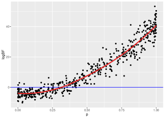
(a) Pólya tree Bayes factors when a standard normal is used for quantiles.

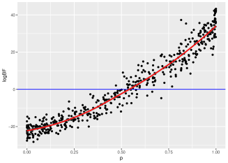
(b) Pólya tree Bayes factors when a standard Cauchy is used for quantiles.

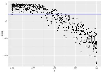
(c) KS test log $P$-values

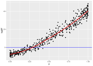
(d) Cross-validation Bayes factors.

Figure 5: Comparison of tests in the scale change case. The densities $f$ and $g$ are both normal in this case.

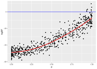
(a) Pólya tree Bayes factors when a standard normal is used for quantiles.

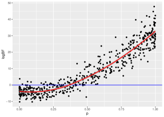
(b) Pólya tree Bayes factors when a standard Cauchy is used for quantiles.

(c) KS test log $P$-values

(d) Cross-validation Bayes factors.

Figure 6: Comparison of tests in the location shift case. The densities $f$ and $g$ are both Cauchy in this case.

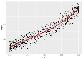
(a) Pólya tree Bayes factors when a standard normal is used for quantiles.

(b) Pólya tree Bayes factors when a standard Cauchy is used for quantiles.

(c) KS test log $P$-values

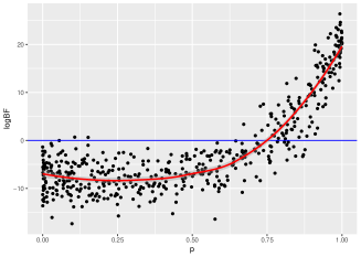
(d) Cross-validation Bayes factors.

Figure 7: Comparison of tests in the case of distributions with different tail behavior. Here $f$ and $g$ are Cauchy and normal, respectively.

(a) Pólya tree Bayes factors when a standard normal is used for quantiles.

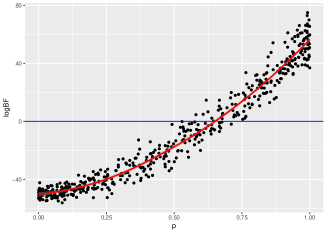
(b) Pólya tree Bayes factors when a standard Cauchy is used for quantiles.

(c) KS test log $P$-values

(d) Cross-validation Bayes factors.

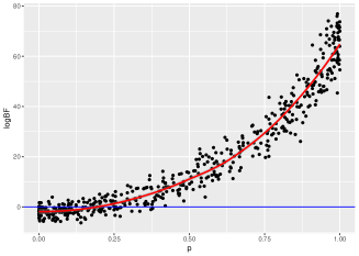
(e) Data-reflected versions of cross-validation Bayes factors. The nonparametric estimate of standard deviation estimate is 5.06. (See text for more detail.)

Figure 8: Comparison of tests in the case of different distributions with same finite support. Here $f$ and $g$ are $U(0,1)$ and beta$(1/2,1/2)$, respectively.

	Pólya tree: Normal	Pólya tree: Cauchy
Setting	base distribution	base distribution	CVBF
Scale change	3.87	4.25	3.39
Location shift	5.49	4.56	4.21
Different tail behavior	4.31	2.89	3.56
Finite support	5.78	6.48	4.45

Table 3: Estimated standard deviations of log-Bayes factors.

Figures 5-8 provide a comparison of CVBFs, Pólya tree Bayes factors and $P$-values of KS tests, where each of the three quantities is on the (natural) log scale. A blue line represents what can be considered the cut-off between evidence favoring one hypothesis over the other. In the case of the KS test the line is at $\text{log}(.05)$, which is often considered to be the largest level of significance for which the null hypothesis should be rejected. For the Bayes factors, the blue lines are at 0, as a log-Bayes factor less than 0 favors the null hypothesis (of equal densities) and one greater than 0 favors the alternative.

To perform the Pólya Tree test, specification of a precision parameter and a base distribution are required. Hanson (2006) recommends centering and scaling the data and using a standard normal distribution as the base distribution. However, doing so turns out not to be efficient when the underlying distribution has sufficiently heavy tails. In the location shift case, for example, the Cauchy density turns out to be far better suited for the base distribution than the normal density since the original density is itself Cauchy. Holmes et al. (2015) provide a data-driven procedure for choosing a base distribution, but do not show that the resulting Bayes factor is consistent under the alternative. For this reason, as well as the fact that the conditional procedure is more computationally intensive, we specify a base distribution, and study its effects. We computed Pólya tree Bayes factors for both normal and Cauchy base distributions in each of the four settings.

The following remarks are in order concerning the simulations under alternatives. To facilitate the discussion, we refer to the Pólya tree methodology based on normal and Cauchy base distributions as PN and PC, respectively.

• In general, the average Pólya tree log-Bayes factor tends to increase as the mixing parameter increases, but, depending on the base distribution, it does not rise above 0 until the mixing parameter is relatively large. This entails that a frequentist strategy would sometimes be needed to ensure good power for a test based on the Pólya tree methodology.

• The behavior of the Pólya tree Bayes factors definitely depends on the base distribution used. Worse yet, the PN Bayes factors performed very poorly when at least one of $f$ and $g$ was Cauchy. In contrast, the performance of CVBFs based on the kernel $K_{0}$ was always comparable to or better than that of both PN and PC.

• The PC Bayes factors performed reasonably well in all four settings, suggesting that the Cauchy might be a good default choice of base distribution. However, the performance of PC in the finite support setting was not nearly as good as that of PN and CVBF. Also, PC Bayes factors were usually more variable than the PN Bayes factors, suggesting that PC may be less powerful in a frequentist sense than PN.

• Taken together, the last two remarks suggest that $K_{0}$ is at least a very good candidate for default kernel choice in the CVBF methodology, whereas identifying a good default base distribution in the Pólya tree methodology is more of an open question.

• Comparing the KS tests with the Bayes tests is not easily done since the interpretation of the $P$-value is so much different than that of a Bayes factor. However, in the case where $f$ and $g$ differed in terms of tail behavior (Figure 7), the behavior of PC and CVBF was clearly better than that of the KS test.

• Table 3 provides estimated standard deviations for the log-Bayes factors (assuming homoscedasticity over the mixing parameter $p$). Each standard deviation is the square root of the following nonparametric variance estimate: $\sum_{i=2}^{500}(b_{i}-b_{i-1})^{2}/1000$, where $b_{i}$ is the log-Bayes factor at $p_{(i)}$, $i=1,\ldots,500$, and $p_{(1)}<p_{(2)}<\cdots<p_{(500)}$ denote the ordered values of the randomly selected mixing parameters. In most cases, the variability of the log-CVBF values is smaller than that of the Pólya tree log-Bayes factors. Importantly, the smaller variability of CVBF is understated as only thirty splits of each data set were used. Recall that in the null case the standard deviations of log-CVBF were about 3/4 of the standard deviations of the Pólya tree log-Bayes factors. So, in addition to often providing more evidence in favor of the correct hypothesis, CVBF appears, in most cases, to be more stable than the Pólya tree method.

• In the finite support case (Figure 8), there are two sets of CVBF results. One set is obtained as in the other three cases, and the other set uses methodology that adjusts kernel estimates for boundary effects. Kernel estimates are known to have large bias near a boundary when the density is positive at the boundary. To deal with the boundary bias we used a data reflection technique. First, we applied the $-\log$ transformation to each of the training data values (which yields exponential data when the underlying distribution is $U(0,1)$). We then reflected these transformed data across the $y$-axis, and constructed a kernel density estimate from a combination of the original and reflected data. Doing so improved the behavior of the log-Bayes factors remarkably. In general this illustrates another point: methods of improving the kernel density estimate may be applied, and doing so can positively impact the log Bayes factors. While this also seems to be the case when choosing which base distribution should be used for the Pólya tree test, we assert that there is more literature on modification of kernel density estimates than for fine-tuning Pólya tree base distributions. See, for example, Kraft et al. (1985), Cowling and Hall (1996), and Bai et al. (1988).

7 Data analysis

We now apply our method to the Higgs boson data set that is available from the UCL Machine Learning repository. The original data set is quite large. It has 29 columns and 11 million rows. The first column is a 0-1 variable indicating whether the data are noise or signal, and the rest of the columns are variables used for distinguishing between noise and signal. The 2nd to 22nd columns consist of predictors, while the 23rd to 29th columns are functions of columns 2 to 22 that are typically used for classification. We will illustrate our methodology by applying it to the data in columns 23 and 29.

Figure 9 provides KDEs for the signal and noise data in column 29. These estimates use all 11,000,000 rows of the data set. Since the two estimates are quite different one would hope that application of our methodology to even ”moderate” sized samples from the two groups would tend to support the hypothesis of unequal densities. To investigate this question, we randomly selected 20,000 rows of the column 29 data. This resulted in $m=9543$ and $n=10,457$ noise and signal observations, respectively. Training set sizes $r=s=1000,2000,3000,4000,5000$ were considered, and $CVBF$ was computed for 20 different random data splits at each $r$. The resulting values are provided in Figure 11. Regardless of the training set size, the evidence in favor of a difference between signal and noise distributions is overwhelming. Interestingly, the results are in agreement with expression (10), which suggests that when the alternative is true, the weight of evidence in favor of the alternative tends to decrease with an increase in training set sizes. These results are consistent with those from the Pólya tree and KS tests. The log-Bayes factor for the Pólya tree test was 234.7242, while the $P$-value from the KS test was essentially 0.

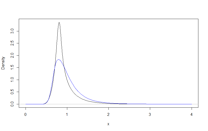
Figure 9: Kernel density estimates for column 29 of the Higgs boson data. The blue curve is for the noise data and the black for signal.

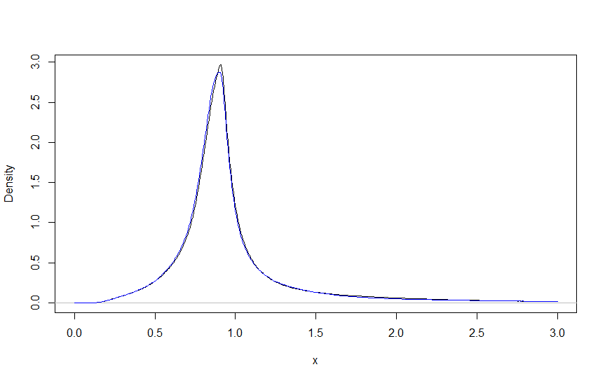
Figure 10: Kernel density estimates for column 23 of the Higgs boson data. The blue curve is for the noise data and the black for signal.

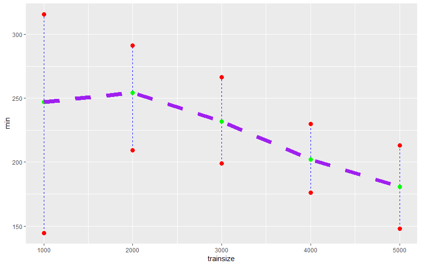
Figure 11: Values of log-CVBF computed from column 29 of the Higgs boson data. The lines connect the averages of log-CVBF at different training set sizes.

We now consider the column 23 data. Figure 10 shows signal and noise KDEs computed from all 11 million data. Since the difference between the two estimates is extremely small, it would not be surprising if Bayes factors based on a small subset of the data support the hypothesis of equal densities. Proceeding exactly as in the case of column 29 data produced the results in Figure 12, where it is seen that all the log-Bayes factors computed were smaller than $-15$. This figure shows that the average of log-$CVBF$ increases as the training set size increases. Based on expression (9), this agrees with what we expect under the null hypothesis of equal distributions. We also considered the use of the Pólya tree and K-S tests on the column 23 data. These methods reach the same basic conclusion as our procedure. The log-Bayes factor of the Pólya tree test was -263.6514, which is in strong favor of the null hypothesis, and the $P$-value of the KS test is 0.1115, which is typically viewed as not small enough to reject the null hypothesis. We also tried the approach outlined at the end of Section 5. We used a prior that assigned equal probability to each of the following training set sizes for both noise and signal observations: 1000, 1190, 1415, 1684, 2003, 2383, 2834, 3372, 4011 and 4772, values that increase approximately linearly on a log scale. One training set for each of the ten sizes was randomly selected, and the Bayes factor (11) was calculated. This procedure was repeated ten times, leading to ten different Bayes factors of the form (11), the average of which was -53.22.

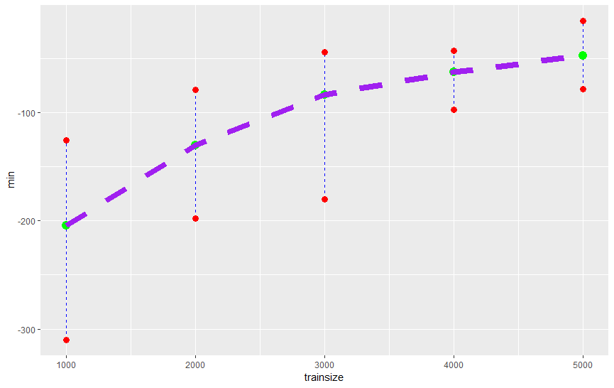
Figure 12: Values of log-CVBF computed from column 23 of the Higgs boson data. The lines connect the averages of log-CVBF at different training set sizes.

Although our focus has been on testing, it is of some interest to see how our cross-validatory methodology compares with Pólya trees in estimating the underlying densities. To this end we compute posterior predictive densities for the column 23 noise data using both our methodology and Pólya trees. Denote the first 9543 values of the column 23 noise data by $x_{1},\ldots,x_{9543}$. In regard to our cross-validation method, the posterior distribution of the bandwidth is

$$\pi(h|\mbox{\boldmath$x$}_{V})\propto\pi(h)\prod_{i=5001}^{9543}\hat{f}(x_{i}|h,\mbox{\boldmath$x$}_{T}),$$

where $\mbox{\boldmath$x$}_{T}=(x_{1},\ldots,x_{5000})$ are the training data and $\mbox{\boldmath$x$}_{V}=(x_{5001},\ldots,x_{9543})$ the validation data. We drew 250 values, $h_{1},\ldots,h_{250}$, from $\pi(\,\cdot\,|\mbox{\boldmath$x$}_{V})$ using an independence-sampler version of Metropolis-Hastings with a normal proposal distribution that was a close match to the posterior. Our approximation $p_{\rm pred}$ of the posterior predictive density was

$$p_{\rm pred}(x)=\frac{1}{250}\sum_{i=1}^{250}\hat{f}(x|h_{i},\mbox{\boldmath$x$}_{T}),$$

which is plotted in Figure 13 along with the Pólya tree posterior predictive density.

Figure 13: Plots of posterior predictive densities for the column 23 Higgs boson noise data. The black line is a KDE based on all 5,170,877 noise data. Because of the size of the data set, we regard this KDE as the truth. The red curve is the posterior predictive density corresponding to the Pólya tree method, and in purple is a cross-validation posterior predictive density.

The Pólya tree method is well known for producing spurious modes in the posterior predictive density (Hanson, 2006). This is evident in Figure 13 in the right tail of the Pólya tree density where the data are relatively sparse. The cross-validation density does not seem to be subject to this problem, at least not to the same degree. In any event, the cross-validatory method has produced at least as good an estimate of the underlying density without the necessity of a complex prior distribution. This illustrates a basic tenet of this paper: one may devise a good Bayesian nonparametric procedure that does not depend on a large number of parameters and the attendant prior specification.

8 Discussion

We have proposed and studied a non-parametric, Bayesian two-sample test for checking equality of distributions. The methodology uses cross-validation Bayes factors (CVBFs), defining kernel density estimate models from training data and then calculating a Bayes factor from validation data. It is advocated that a CVBF be used in genuine Bayesian fashion, i.e., by interpreting it as the relative odds of the two hypotheses. This is in contrast to the proposal of Holmes et al. (2015), who evaluate a Pólya tree Bayes factor in frequentist fashion using a permutation test. We argue that the CVBF is Bayes factor consistent under both hypotheses, and under the null hypothesis it converges in probability to 0 at an exceptionally fast rate. We provide a supplementary R package that calculates CVBFs and the Pólya tree Bayes factor of Holmes et al. (2015), assuming that a base distribution is supplied for the latter method.

Depending on how many data splits are utilized, calculating the average of several values of $CVBF$ can be slower than calculating the Pólya tree Bayes factor. In particular, CVBF computations do not scale as well with the size of the data set as do those of the Pólya tree procedure. This is mainly due to the fact that maximizing (with respect to bandwidth) the likelihood of kernel density estimates can be time consuming. A future research problem involves the attempt to speed up the test by utilizing techniques that speed bandwidth selection. There is a great deal of information regarding how to speed up KDE calculations. Binning the data and utilizing bagging to select a bandwidth are methods that can perhaps be used to speed up CVBF calculations.

Finally, it is worth mentioning that the idea of CVBF can be generalized in a fairly straightforward fashion to deal with other inference problems, including comparison of multivariate densities, comparison of more than two densities and comparison of regression functions.

Appendix

Here we derive $\widehat{H}$, as defined at the bottom of p. 8. Let $\hat{f}_{h}$ be a KDE based on data $Z_{1},\ldots,Z_{k}$ and kernel $K$, and for arbitrary scalar quantities $u_{1},\ldots,u_{\ell}$ define $L_{1}$ as follows:

$$L_{1}(h)=\prod_{j=1}^{\ell}\hat{f}_{h}(u_{j}).$$

Then $L_{1}$ has the same structure as $L_{0}$ in Section 3.2, and it suffices to consider

$$\frac{\partial^{2}}{\partial h^{2}}\log L_{1}(h)=\sum_{j=1}^{\ell}\left[\hat{f}_{h}(u_{j})\frac{\partial^{2}}{\partial h^{2}}\hat{f}_{h}(u_{j})-\left(\frac{\partial}{\partial h}\hat{f}_{h}(u_{j})\right)^{2}\right]/\hat{f}_{h}^{2}(u_{j}).$$ (12)

We have

$$\frac{\partial}{\partial h}\hat{f}_{h}(u_{j})=-\frac{1}{h}\left[\hat{f}_{h}(u_{j})-\hat{e}_{h}(u_{j})\right],$$ (13)

where $\hat{e}_{h}$ is a kernel estimator based on data $Z_{1},\ldots,Z_{k}$ and kernel $J(u)=-uK^{\prime}(u)$. Note that $\hat{e}_{h}$ is a “legitimate” kernel estimator in that $\int_{-\infty}^{\infty}J(u)\,du=1$ and $\int_{-\infty}^{\infty}uJ(u)\,du=0$.

Now,

$$\frac{\partial^{2}}{\partial h^{2}}\hat{f}_{h}(u_{j})=-\frac{1}{h}\left[2\frac{\partial}{\partial h}\hat{f}_{h}(u_{j})-\frac{\partial}{\partial h}\hat{e}_{h}(u_{j})\right],$$ (14)

and

$$\frac{\partial}{\partial h}\hat{e}_{h}(u_{j})=-\frac{1}{h}\left[\hat{e}_{h}(u_{j})-\hat{g}_{h}(u_{j})\right],$$

where $\hat{g}_{h}$ is a kernel estimator based on data $Z_{1},\ldots,Z_{k}$ and kernel $L(u)=-uJ^{\prime}(u)$. As before, $\hat{g}_{h}$ is a legitimate, i.e., consistent, density estimator. Substitution of (13) and (14) into (12) leads to a readily computable expression for $\widehat{H}$.

References

- Bai et al. (1988) Bai, Z., C. Rao, and L. Zhao (1988). Kernel estimators of density function of directional data. Journal of Multivariate Analysis 27, 24–39.
- Beirlant et al. (1997) Beirlant, J., E. J. Dudewicz, L. Györfi, and I. Dénes (1997). Nonparametric entropy estimation: An overview. International Journal of Mathematical and Statistical Sciences 6, 17–39.
- Chen and Hanson (2014) Chen, Y. and T. E. Hanson (2014). Bayesian nonparametric -sample tests for censored and uncensored data. Computational Statistics & Data Analysis 71, 335–346.
- Consonni et al. (2018) Consonni, G., D. Fouskakis, B. Liseo, I. Ntzoufras, et al. (2018). Prior distributions for objective Bayesian analysis. Bayesian Analysis 13, 627–679.
- Cowling and Hall (1996) Cowling, A. and P. Hall (1996). On pseudodata methods for removing boundary effects in kernel density estimation. Journal of the Royal Statistical Society B 58, 551–563.
- Dunson and Peddada (2008) Dunson, D. B. and S. D. Peddada (2008). Bayesian nonparametric inference on stochastic ordering. Biometrika 95, 859–874.
- Györfi et al. (1985) Györfi, L., L. Devroye, and L. Gyorfi (1985). Nonparametric density estimation: the L1 view. New York; Chichester: John Wiley & Sons.
- Hall (1987) Hall, P. (1987). On Kullback-Leibler loss and density estimation. Annals of Statistics 15, 1491–1519.
- Hanson (2006) Hanson, T. E. (2006). Inference for mixtures of finite Pólya tree models. Journal of the American Statistical Association 101, 1548–1565.
- Hart (2017) Hart, J. D. (2017). Use of BayesSim and smoothing to enhance simulation studies. Open Journal of Statistics 7, 153–172.
- Hart and Choi (2017) Hart, J. D. and T. Choi (2017). Nonparametric goodness of fit via cross-validation Bayes factors. Bayesian Analysis 12, 653–677.
- Hart and Malloure (2019) Hart, J. D. and M. Malloure (2019). Prior-free Bayes factors based on data splitting. International Statistical Review 87, 419–442.
- Holmes et al. (2015) Holmes, C. C., F. Caron, J. E. Griffin, D. A. Stephens, et al. (2015). Two-sample Bayesian nonparametric hypothesis testing. Bayesian Analysis 10, 297–320.
- Kass and Raftery (1995) Kass, R. E. and A. E. Raftery (1995). Bayes factors. Journal of the American Statistical Association 90, 773–795.
- Kraft et al. (1985) Kraft, C., Y. Lepage, and C. Van Eeden (1985). Estimation of a symmetric density function. Communications in Statistics–Theory and Methods 14, 273–288.
- McVinish et al. (2009) McVinish, R., J. Rousseau, and K. Mengersen (2009). Bayesian goodness of fit testing with mixtures of triangular distributions. Scandinavian Journal of Statistics 36, 337–354.
- Sarkar and Goswami (2013) Sarkar, S. D. and S. Goswami (2013). Empirical study on filter based feature selection methods for text classification. International Journal of Computer Applications 81.
- van der Laan et al. (2004) van der Laan, M., S. Dudoit, and S. Keleş (2004). Asymptotic optimality of likelihood-based cross-validation. Statistical Applications in Genetics and Molecular Biology 3, online publication.
- Wong et al. (2010) Wong, W. H., L. Ma, et al. (2010). Optional Pólya tree and Bayesian inference. The Annals of Statistics 38, 1433–1459.