An Evaluation of Change Point Detection Algorithms

Abstract

Change point detection is an important part of time series analysis, as the presence of a change point indicates an abrupt and significant change in the data generating process. While many algorithms for change point detection have been proposed, comparatively little attention has been paid to evaluating their performance on real-world time series. Algorithms are typically evaluated on simulated data and a small number of commonly-used series with unreliable ground truth. Clearly this does not provide sufficient insight into the comparative performance of these algorithms. Therefore, instead of developing yet another change point detection method, we consider it vastly more important to properly evaluate existing algorithms on real-world data. To achieve this, we present a data set specifically designed for the evaluation of change point detection algorithms that consists of 37 time series from various application domains. Each series was annotated by five human annotators to provide ground truth on the presence and location of change points. We analyze the consistency of the human annotators, and describe evaluation metrics that can be used to measure algorithm performance in the presence of multiple ground truth annotations. Next, we present a benchmark study where 14 algorithms are evaluated on each of the time series in the data set. Our aim is that this data set will serve as a proving ground in the development of novel change point detection algorithms.
Keywords: change point detection, time series analysis, benchmark evaluation

1 Introduction

Moments of abrupt change in the behavior of a time series are often cause for alarm as they may signal a significant alteration to the data generating process. Detecting such change points is therefore of high importance for data analysts and engineers. The literature on change point detection (CPD) is concerned with accurately detecting these events in time series data, as well as with modeling time series in which such events occur. Applications of CPD are found in finance (Lavielle and Teyssiere, 2007), business (Taylor and Letham, 2018), quality control (Page, 1954), and network traffic analysis (Kurt et al., 2018), among many other domains.

There is a large body of work on both the theoretical and practical aspects of change point detection. However, less attention has been paid to the evaluation of CPD algorithms on real-world time series. Existing work often follows a predictable strategy when presenting a novel detection algorithm: the method is first evaluated on a set of simulated time series with known change points where both the model fit and detection accuracy are evaluated. An obvious downside of such experiments is that the dynamics of the simulated data are often particular to the paper, and any model that corresponds to these dynamics has an unfair advantage. Subsequently the proposed method is typically evaluated on only a small number of real-world time series. These series are often reused (e.g., the univariate well-log data of Ó Ruanaidh and Fitzgerald, 1996), may have been preprocessed (e.g., by removing outliers or seasonality), and may not have unambiguous ground truth available. When evaluating a proposed method on real-world data, post-hoc analysis is frequently applied to argue why the locations detected by the algorithm correspond to known events. Clearly, this is not a fair or accurate approach to evaluating novel change point detection algorithms.

Rather than proposing yet another detection method and evaluating it in the manner just described, we argue that it is vastly more important to create a realistic benchmark data set for CPD algorithms. Such a data set will allow researchers to evaluate their novel algorithms in a systematic and realistic way against existing alternatives. Furthermore, since change point detection is generally an unsupervised learning problem, an evaluation on real-world data is the most reliable approach to properly compare detection accuracy. A benchmark data set can also uncover important failure modes of existing methods that may not occur in simulated data, and suggest avenues for future research based on a quantitative analysis of algorithm performance.

Change point detection can be viewed as partitioning an input time series into a number of segments. It is thus highly similar to the problem of image segmentation, where an image is partitioned into distinct segments based on different textures or objects. Historically, image segmentation suffered from the same problem as change point detection does today, due to the absence of a large, high-quality data set with objective ground truth (as compared to, for instance, image classification). It was not until the Berkeley Segmentation Data Set (BSDS; Martin et al., 2001) that quantitative comparison of segmentation algorithms became feasible. We believe that it is essential to develop a similar data set for change point detection, to enable both the research community as well as data analysts to quantitatively compare CPD algorithms.

To achieve this goal, we present the first data set specifically designed to evaluate change point detection algorithms that consists of time series from diverse application domains. We developed an annotation tool and collected annotations from data scientists for 37 real-world time series. Using this data set, we perform a large-scale quantitative evaluation of existing algorithms. We analyze the results of this comparison to uncover failure cases of present methods and discuss various potential improvements. To summarize, our main contributions are as follows.

1. We describe the design and collection of a data set for change point detection algorithms and analyze the data set for annotation quality and consistency. The data set is made freely available to accelerate research on change point detection.

2. We present metrics for the evaluation of change point detection algorithms that take multiple annotations per data set into account.

3. We evaluate a significant number of existing change point detection algorithms on this data set and provide the first benchmark study on a large number of real-world data sets using two distinct experimental setups.

The remainder of this paper is structured as follows. In Section 2 we give a high-level overview and categorization of existing work on CPD. Section 3 presents a framework for evaluating change point methods when ground truth from multiple human annotators is available. The annotation tool and data set collection process are described in Section 4, along with an analysis of data quality and annotator consistency. The design of the benchmark study and an analysis of the results is presented in Section 5. Section 6 concludes.

2 Related Work

Methods for CPD can be roughly categorized as follows: (1) online vs. offline, (2) univariate vs. multivariate, and (3) model-based vs. nonparametric. We can further differentiate between Bayesian and frequentist approaches among the model-based methods, and between divergence estimation and heuristics in the nonparametric methods. Due to the large amount of work on CPD we only provide a high-level overview of some of the most relevant methods here, which also introduces many of the methods that we subsequently consider in our evaluation study. For a more expansive review of change point detection algorithms, see e.g., Aminikhanghahi and Cook (2017) or Truong et al. (2020). Note that we focus here on the unsupervised change point detection problem, without access to external data that can be used to tune hyperparameters (Hocking et al., 2013a; Truong et al., 2017).

Let $\mathbf{y}_{t}\in\mathcal{Y}$ denote the observations for time steps $t=1,2,\ldots$, where the domain $\mathcal{Y}$ is $d$-dimensional and typically assumed to be a subset of $\mathbb{R}^{d}$. A segment of the series from $t=a,a+1,\ldots,b$ will be written as $\mathbf{y}_{a:b}$. The ordered set of change points is denoted by $\mathcal{T}=\{\tau_{0},\tau_{1},\ldots,\tau_{n}\}$, with $\tau_{0}=1$ for notational convenience. In offline change point detection we further use $T$ to denote the length of the series and define $\tau_{n+1}=T+1$. Note that we assume that a change point marks the first observation of a new segment.

Early work on CPD originates from the quality control literature. Page (1954) introduced the CUSUM method that detects where the corrected cumulative sum of observations exceeds a threshold value. Theoretical analysis of this method was subsequently provided by Lorden (1971). Hinkley (1970) generalized this approach to testing for differences in the maximum likelihood, i.e., testing whether $\log p(\mathbf{y}_{1:T}\;|\;\theta)$ and $\max_{\tau}[\log p(\mathbf{y}_{1:\tau-1}\;|\;\theta_{1})+\log p(\mathbf{y}_{\tau:T}\;|\;\theta_{2})]$ differ significantly, for model parameters $\theta$, $\theta_{1}$, and $\theta_{2}$. Alternatives from the literature on structural breaks include the use of a Chow test (Chow, 1960) or multiple linear regression (Bai and Perron, 2003).

In offline multiple change point detection the optimization problem is given by

$$\min_{\mathcal{T}}\sum_{i=1}^{n+1}\ell(\mathbf{y}_{\tau_{i-1}:\tau_{i}-1})+\lambda P(n),$$ (1)

with $\ell(\cdot)$ a cost function for a segment (e.g., the negative maximum log-likelihood), $\lambda\geq 0$ a hyperparameter, and $P(n)$ a penalty on the number of change points. An early method by Scott and Knott (1974) introduced binary segmentation as an approximate CPD algorithm that greedily splits the series into disjoint segments based on the above cost function. This greedy method thus obtains a solution in $\mathcal{O}(T\log T)$ time. An efficient dynamic programming approach to compute an exact solution for the multiple change point problem was presented in Auger and Lawrence (1989), with $\mathcal{O}(mT^{2})$ time complexity for a given upper bound $m$ on the number of change points.

Improvements to these early algorithms were made by requiring the cost function to be additive, i.e., $\ell(\mathbf{y}_{a:b})=\ell(\mathbf{y}_{a:\tau-1})+\ell(\mathbf{y}_{\tau:b})$. Using this assumption, Jackson et al. (2005) present a dynamic programming algorithm with $\mathcal{O}(T^{2})$ complexity. Killick et al. (2012) subsequently extended this method with a pruning step on potential change point locations, which reduces the time complexity to be approximately linear under certain conditions on the data generating process and the distribution of change points. A different pruning approach was proposed by Rigaill (2015) using further assumptions on the cost function, which was extended by Maidstone et al. (2017) and made robust against outliers by Fearnhead and Rigaill (2019). Recent work in offline CPD also includes the Wild Binary Segmentation method (Fryzlewicz, 2014) that extends binary segmentation by applying the CUSUM statistic to randomly drawn subsets of the time series. Furthermore, the Prophet method for Bayesian time series forecasting (Taylor and Letham, 2018) supports fitting time series with change points, even though it is not a dedicated CPD method. These offline detection methods are generally restricted to univariate time series.

Bayesian online change point detection was simultaneously proposed by Fearnhead and Liu (2007) and Adams and MacKay (2007). These models learn a probability distribution over the “run length”, which is the time since the most recent change point. This gives rise to a recursive message-passing algorithm for the joint distribution of the observations and the run lengths. The formulation of Adams and MacKay (2007) has been extended in several works to include online hyperparameter optimization (Turner et al., 2009) and Gaussian Process segment models (Garnett et al., 2009; Saatçi et al., 2010). Recent work by Knoblauch and Damoulas (2018) has added support for model selection and spatio-temporal models, as well as robust detection using $\beta$-divergences (Knoblauch et al., 2018).

Nonparametric methods for CPD are typically based on explicit hypothesis testing, where a change point is declared when a test statistic exceeds a certain threshold. This includes kernel change point analysis (Harchaoui et al., 2009), the use of an empirical divergence measure (Matteson and James, 2014), as well as the use of histograms to construct a test statistic (Boracchi et al., 2018). Both the Bayesian online change point detection methods and the nonparametric methods support multidimensional data.

Finally, we observe that in the field of genomics a number of data sets exist that can be used to evaluate change point detection methods (e.g., Hocking et al., 2013a, b, 2014). While this is an important application domain for CPD algorithms, we are interested in evaluating the performance of change point algorithms on general real-world time series from diverse domains. Moreover, the data sets proposed in Hocking et al. (2013b, 2014) make use of labeled regions that are annotated as containing a change point or not, instead of labels of the exact change point locations. While in this work exact labels are preferred over labeled regions, the latter can certainly simplify the annotation task for longer time series. We allow a small margin of error in the evaluation metrics to take any potential uncertainty of the annotators into account.

3 Evaluation Metrics

In this section we review common metrics for evaluating CPD algorithms and provide those that can be used to compare algorithms against multiple ground truth annotations. These metrics will also be used to quantify the consistency of the annotations of the time series, which is why they are presented here. Our discussion bears many similarities to that provided by Martin et al. (2004) and Arbelaez et al. (2010) for the BSDS, due to the parallels between change point detection and image segmentation.

Existing metrics for change point detection can be roughly divided between clustering metrics and classification metrics. These categories represent distinct views of the change point detection problem, and we discuss them in turn. The locations of change points provided by annotator $k\in\{1,\ldots,K\}$ are denoted by the ordered set $\mathcal{T}_{k}=\left\{\tau_{1},\ldots,\tau_{n_{k}}\right\}$ with $\tau_{i}\in[1,T]$ for $i=1,\ldots,n_{k}$ and $\tau_{i}<\tau_{j}$ for $i<j$. Then $\mathcal{T}_{k}$ implies a partition, $\mathcal{G}_{k}$, of the interval $[1,T]$ into disjoint sets $\mathcal{A}_{j}$, where $\mathcal{A}_{j}$ is the segment from $\tau_{j-1}$ to $\tau_{j}-1$ for $j=1,\ldots,n_{k}+1$. Recall that we use $\tau_{0}=1$ and $\tau_{n_{k}+1}=T+1$ for notational convenience.

Evaluating change point algorithms using clustering metrics corresponds to the view that change point detection inherently aims to divide the time series into distinct regions with a constant data generating process. Clustering metrics such as the variation of information (VI; Arabie and Boorman, 1973), adjusted Rand index (ARI; Hubert and Arabie, 1985), Hausdorff distance (Hausdorff, 1927), and segmentation covering metric (Everingham et al., 2010; Arbelaez et al., 2010) can be readily applied. We disregard the Hausdorff metric because it is a maximum discrepancy metric and can therefore obscure the true performance of methods that report many false positives. Following the discussion in Arbelaez et al. (2010) regarding the difficulty of using VI for multiple ground truth partitions and the small dynamic range of the Rand index, we choose to use the covering metric as the clustering metric in the experiments.

For two sets $\mathcal{A},\mathcal{A}^{\prime}\subseteq[1,T]$ the Jaccard index, also known as Intersection over Union, is given by

$$J(\mathcal{A},\mathcal{A}^{\prime})=\frac{\left|\mathcal{A}\cap\mathcal{A}^{\prime}\right|}{\left|\mathcal{A}\cup\mathcal{A}^{\prime}\right|}.$$ (2)

Following Arbelaez et al. (2010), we define the covering metric of a partition $\mathcal{G}$ by a partition $\mathcal{G}^{\prime}$ as

$$C(\mathcal{G},\mathcal{G}^{\prime})=\frac{1}{T}\sum_{\mathcal{A}\in\mathcal{G}}\left|\mathcal{A}\right|\cdot\max_{\mathcal{A}^{\prime}\in\mathcal{G}^{\prime}}J(\mathcal{A},\mathcal{A}^{\prime}).$$ (3)

For a collection $\left\{\mathcal{G}_{k}\right\}_{k=1}^{K}$ of ground truth partitions provided by the human annotators and a partition $\mathcal{S}$ given by an algorithm, we compute the average of $C(\mathcal{G}_{k},\mathcal{S})$ for all annotators as a single measure of performance.

An alternative view of evaluating CPD algorithms considers change point detection as a classification problem between the “change point” and “non-change point” classes (Killick et al., 2012; Aminikhanghahi and Cook, 2017). Because the number of change points is generally a small proportion of the number of observations in the series, common classification metrics such as the accuracy score will be highly skewed. It is more useful to express the effectiveness of an algorithm in terms of precision (the ratio of correctly detected change points over the number of detected change points) and recall (the ratio of correctly detected change points over the number of true change points). The $F_{\beta}$-measure provides a single quantity that incorporates both precision, $P$, and recall, $R$, through

$$F_{\beta}=\frac{(1+\beta^{2})PR}{\beta^{2}P+R},$$ (4)

with $\beta=1$ corresponding to the well-known F1-score (Van Rijsbergen, 1979).

When evaluating CPD algorithms using classification metrics it is common to define a margin of error around the true change point location to allow for minor discrepancies (e.g., Killick et al., 2012; Truong et al., 2020). However with this margin of error we must be careful to avoid double counting, so that for multiple detections within the margin around a true change point only one is recorded as a true positive (Killick et al., 2012). To handle the multiple sets of ground truth change points provided by the annotator, we follow the precision-recall framework from the BSDS proposed in Martin et al. (2004). Let $\mathcal{X}$ denote the set of change point locations provided by a detection algorithm and let $\mathcal{T}^{*}=\bigcup_{k}\mathcal{T}_{k}$ be the combined set of all human annotations. For a set of ground truth locations $\mathcal{T}$ we define the set of true positives $\text{TP}(\mathcal{T},\mathcal{X})$ of $\mathcal{X}$ to be those $\tau\in\mathcal{T}$ for which $\exists x\in\mathcal{X}$ such that $\left|\tau-x\right|\leq M$, while ensuring that only one $x\in\mathcal{X}$ can be used for a single $\tau\in\mathcal{T}$. The latter requirement is needed to avoid the double counting mentioned previously, and $M\geq 0$ is the allowed margin of error. The precision and recall are then defined as

$$P =\frac{\left|\text{TP}(\mathcal{T}^{*},\mathcal{X})\right|}{\left|\mathcal{X}\right|},$$ (5)

$$R =\frac{1}{K}\sum_{k=1}^{K}\frac{\left|\text{TP}(\mathcal{T}_{k},\mathcal{X})\right|}{\left|\mathcal{T}_{k}\right|}.$$ (6)

With this definition of precision, we consider as false positives only those detections that correspond to no human annotation. Further, by defining the recall as the average of the recall for each individual annotator we encourage algorithms to explain all human annotations without favoring any annotator in particular. Note that precision and recall are undefined if the annotators or the algorithm declare that a series has no change points. To avoid this, we include $t=1$ as a trivial change point in $\mathcal{T}_{k}$ and $\mathcal{X}$. Since change points are interpreted as the start of a new segment this choice does not affect the meaning of the detection results.

Using both the segmentation covering metric and the F1-score in the benchmark study allows us to explore both the clustering and classification view of change point detection. In the experiments we use a margin of error of $M=5$.

4 Change Point Data Set

This section describes the tool used in collecting the change point annotations, as well as the data sources, the experimental protocol, and an analysis of the obtained annotations.

4.1 Annotation Tool

To facilitate the collection of the annotated data set, we created a web application that enables annotators to mark change points on a plot of a time series (see Figure 1). Annotators can select multiple change points in the data or can signal that they believe the time series contains no change points. The application allows the annotators to zoom in and pan to particular sections of the time series for closer inspection. Before annotators are provided with any real-world time series, they are required to go through a set of introductory pages that describe the application and show various types of change points (including changes in mean, variance, trend, and seasonality). These introductory pages also illustrate the difference between a change point and an outlier. During this introduction the annotator is presented with several synthetic time series with known change points and provided with feedback on the accuracy of their annotations. If the annotator’s average F1-score is too low on these introductory data sets, they are kindly asked to repeat the introduction. This ensures that all annotators have a certain baseline level of familiarity with annotating change points.

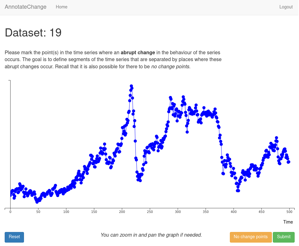
Figure 1: The annotation tool created to collect time series annotations. Note that no contextual information of the time series is provided to ensure annotators do not use external knowledge during the process. The rubric presented to the annotators is also visible.

To avoid that annotators use their knowledge of historical events or are affected by other biases, no dates are shown on the time axis and no values are present on the vertical axis. The names of the series are also not shown to the annotators. Furthermore, the annotation page always displays the following task description to the annotators:

Please mark the point(s) in the time series where an abrupt change in the behavior of the series occurs. The goal is to define segments of the time series that are separated by places where these abrupt changes occur. Recall that it is also possible for there to be no change points.

This description is purposefully left somewhat vague to avoid biasing the annotators in a specific direction, and is inspired by the rubric in the BSDS (Martin et al., 2001).

4.2 Data Sources

Time series were collected from various online sources including the WorldBank, EuroStat, U.S. Census Bureau, GapMinder, and Wikipedia. A number of time series show potential change point behavior around the financial crisis of 2007–2008, such as the price for Brent crude oil (Figure 1), U.S. business inventories, and U.S. construction spending, as well as the GDP series for various countries. Other time series are centered around introduced legislation, such as the mandatory wearing of seat belts in the U.K., the Montreal Protocol regulating CFC emissions, or the regulation of automated phone calls in the U.S. Various data sets are also collected from existing work on change point detection and structural breaks, such as the well-log data set (Ó Ruanaidh and Fitzgerald, 1996), a Nile river data set (Durbin and Koopman, 2012), and a sequence from the bee-waggle data set (Oh et al., 2008). The main criterion for including a time series was whether it displayed interesting behavior that might include an abrupt change. Several time series were included that may not in fact contain a change point but are nevertheless considered interesting for evaluating CPD algorithms due to features such as seasonality or outliers.

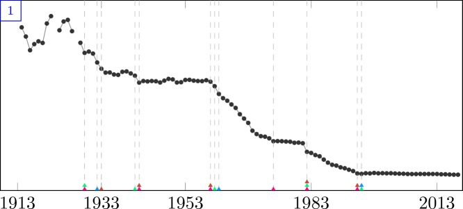
Figure 37: Number of workers employed in British coal mines. Data obtained from the U.K. government.

A total of 37 real time series were collected for the change point data set. This includes 33 univariate and 4 multivariate series (with either 2 or 4 dimensions). One of the univariate time series (uk_coal_employ, Figure 37 in Appendix D) has two missing observations, and nine other series show seasonal patterns. Unbeknownst to the annotators we added 5 simulated “quality control” series with known change points in the data set, which allows us to evaluate the quality of the annotators in situ (see below). Four of these series have a change point with a shift in the mean and the fifth has no change points. Of the quality control series with a change point two have a change in noise distribution, one contains an outlier, and another has multiple periodic components. The change point data set thus consists of 42 time series in total. The average length of the time series in the data set is 327.7, with a minimum of 15 and a maximum of 991. Additional descriptive statistics are provided in Table 4 in Appendix C.1 and visualizations of all series are provided in Appendix D. Note that because we ask the annotators to mark all points in the series that they believe to be change points, we have chosen time series for which this task is feasible.

4.3 Annotation Collection

Annotations were collected in several sessions by inviting data scientists and machine learning researchers to annotate the series. We deliberately chose not to ask individuals who have extensive background knowledge on the various domains of the time series, as this could affect the objectivity of their annotations. For example, asking someone who is familiar with oil prices to annotate the brent_spot series might allow them to use outside knowledge that is not available from the behavior of the series alone. The annotation tool randomly assigned time series to annotators whenever they requested a new series to annotate, with a bias towards series that already had annotations. The same series was never assigned to an annotator more than once. In total, eight annotators provided annotations for the 42 time series, with five annotators assigned to each time series. On average the annotators marked 7.4 unique change points per series, with a standard deviation of 7.0, a minimum of 0 and a maximum of 26. The provided annotations for each series are shown in Appendix D.

Although all annotators successfully completed the introduction before annotating any real time series, some nonetheless commented on the difficulty of deciding whether a series had a change point or not. In some cases this was due to a significant change spanning multiple time steps, which led to ambiguity about whether the transition period should be marked as a separate segment or not (see e.g., Figure 1). Another source of ambiguity were periodic time series with abrupt changes (e.g., bank, Figure 6), which could be regarded as a stationary switching distribution without abrupt changes or a series with frequent change points. In these cases annotators were advised to use their intuition and experience as data scientists to evaluate whether they considered a potential change to be an abrupt change. Note that uncertainty in the exact position of an annotation is partially alleviated by the margin of error included in the evaluation metrics (in particular the F1-score, see Section 3).

4.4 Consistency

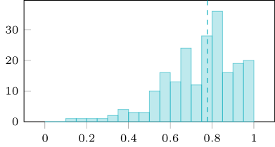
(a)

(b)

Figure 2: Histograms of one vs. rest annotator performance for both metrics. Median scores over all data sets are shown with dashed lines.

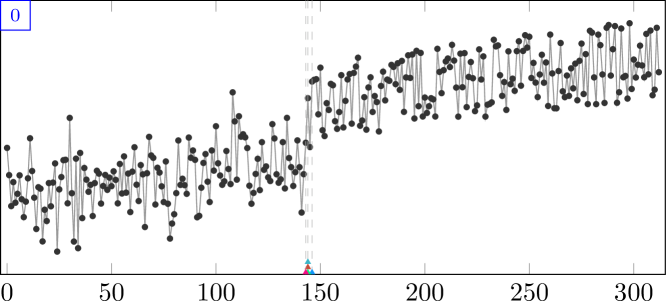
Figure 42: A series with a known change point at index 146. The series has Gaussian noise and a small trend before the change point and an offset and uniform noise after the change point.

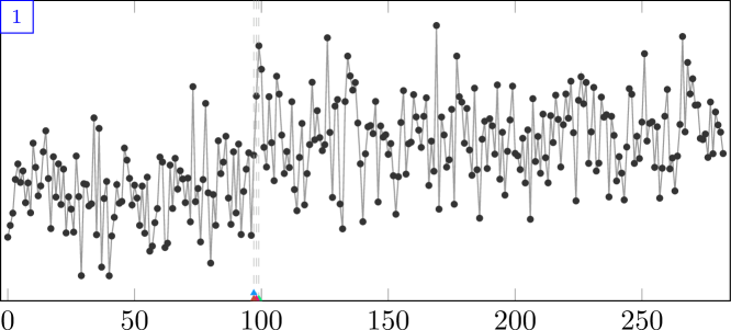
Figure 43: A series with a known change point at index 97. The series has constant noise and a mean shift change point.

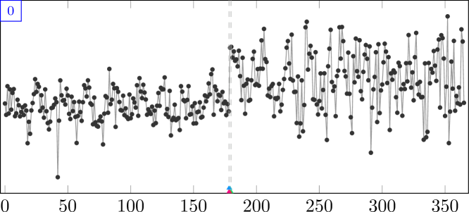
Figure 44: A series with a known change point at index 179. The series has noise $\mathcal{N}(0,1)$ before the change point and $\mathcal{N}(2,2)$ after the change point, as well as an outlier at index 42.

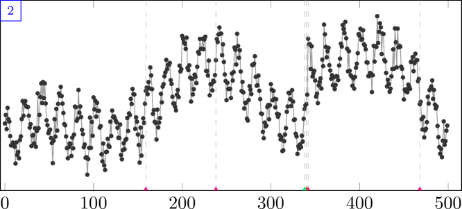
Figure 45: A series with a known change point at index 341. The series has multiple periodic components of different amplitude and a mean shift change point.

As mentioned above we included five “quality control” series to evaluate the accuracy and consistency of the human annotators in practice, which are shown in Appendix D.2. On two of the four series with known change points (Figure 42 and Figure 44) all annotators identified the true change point within three time steps of the correct location. On another time series, quality_control_2, four of the five annotators identified the change point within two time steps, with a fifth annotator believing there to be no change points (Figure 43). The most difficult series to annotate was the one with periodic features (quality_control_4, Figure 45). Here, two of the annotators voted there to be no change points while the three other annotators identified the change correctly within three time steps, with one also incorrectly marking several other points as change points. The series without change points, quality_control_5, was correctly identified as such by all annotators. This suggests that human annotators can identify the presence and location of change points with high accuracy on most kinds of time series, with seasonal effects posing the biggest challenge.

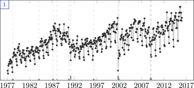
Figure 24: The number of passengers arriving and departing at LaGuardia airport in New York City. Data obtained from the Port Authority of New York and New Jersey.

To quantitatively assess the consistency of the annotators we evaluate each individual annotator against the four others on every time series, using the metrics presented previously. Figure 2 shows the histograms of these one-vs-rest (OvR) scores for both metrics. The figures show that on average there is a high degree of agreement between annotators, with the median annotator score approximately 0.8 for the covering metric and 0.9 for the F1-score (for both metrics a score of 1.0 indicates perfect agreement). It can also be seen that the values are generally higher on the F1-score, which is due to the margin of error in this metric and the fact that the F1-score uses the union of annotated change points in the definition of the precision. In Appendix B we additionally present a simulation study to explore the extent to which the observed annotator agreement can be expected by chance. We find that for both metrics and for the majority of time series the observed average OvR annotator agreement is significantly higher than can be expected by chance. The few cases with low agreement are often due to one or two annotators disagreeing with the others. An example of this is the lga_passengers series, where there is a high level of agreement between four of the annotators about the number and approximate location of the change points, but one annotator believes there are no change points (see Figure 24).

5 Benchmark Study

This section presents a benchmark study of existing change point algorithms on the data set of human-annotated time series. We describe the methods included in the study, the setup of the experiments, and the results of the evaluation. The code and data used in this benchmark study are available through an online repository.

Table 1: The change point detection algorithms considered in the benchmark study.

Name	Method	Reference
amoc	At Most One Change	Hinkley (1970)
binseg	Binary Segmentation	Scott and Knott (1974)
bocpd	Bayesian Online Change Point Detection	Adams and MacKay (2007)
bocpdms	bocpd with Model Selection	Knoblauch and Damoulas (2018)
cpnp	Nonparametric Change Point Detection	Haynes et al. (2017)
ecp	Energy Change Point	Matteson and James (2014)
kcpa	Kernel Change-Point Analysis	Harchaoui et al. (2009)
pelt	Pruned Exact Linear Time	Killick et al. (2012)
prophet	Prophet	Taylor and Letham (2018)
rbocpdms	Robust bocpdms	Knoblauch et al. (2018)
rfpop	Robust Functional Pruning Optimal Partitioning	Fearnhead and Rigaill (2019)
segneigh	Segment Neighborhoods	Auger and Lawrence (1989)
wbs	Wild Binary Segmentation	Fryzlewicz (2014)
zero	No Change Points

5.1 Experimental Setup

The aim of the study is to obtain an understanding of the performance of existing change point methods on real-world data. With that in mind we evaluate a large selection of methods that are either frequently used or that have been recently developed. Table 1 lists the methods included in the study. To avoid issues with implementations we use existing software packages for all methods, which are almost always made available by the authors themselves. We also include the baseline zero method, which always returns that a series contains no change points.

Many of the methods have (hyper)parameters that affect the predicted change point locations. To obtain a realistic understanding of how accurate the methods are in practice, we create two separate evaluations: one showing the performance using the default settings of the method as defined by the package documentation, and one reporting the maximum score over a grid search of parameter configurations. We refer to these settings as the “Default” and “Oracle” experiments, respectively. The Default experiment aims to replicate the common practical setting of a data analyst trying to detect potential change points in a time series without any prior knowledge of reasonable parameter choices. The Oracle experiment aims to identify the highest possible performance of each algorithm by running a full grid search over its hyperparameters. It should be emphasized that while the Oracle experiment is important from a theoretical point of view, it is not necessarily a realistic measure of practical algorithm performance. Due to the unsupervised nature of the change point detection problem we can not in general expect those who use these methods to be able to tune the parameters such that the results match the unknown ground truth. For a detailed overview of how each method was applied, see Appendix A.

Since not all methods support multidimensional time series or series with missing values, we separate the analysis further into univariate and multivariate time series. While it is possible to use the univariate methods on multidimensional time series by, for instance, combining the detected change points of each dimension, we chose not to do this as it could skew the reported performance with results on series that the methods are not explicitly designed to handle. Furthermore, because the programming language differs between implementations we do not report on the computation time of the methods. All series are standardized to zero mean and unit variance to avoid issues with numerical precision arising for some methods on some of the time series. The quality control time series were not included in the benchmark study, but performance on these series is reported in Appendix C.1.

The Bayesian online change point detection algorithms that follow the framework of Adams and MacKay (2007) compute a full probability distribution over the location of the change points and therefore do not return a single segmentation of the series. To allow for comparisons to the other methods we use the maximum a posteriori (MAP) segmentation of the series (see, e.g., Fearnhead and Liu, 2007). The MAP segmentation results in a single set of detected change points that can be compared to those provided by offline methods.

5.2 Results

Table 2: Scores for both experiments on each metric, separated among univariate and multivariate time series. For the Default experiment the value corresponds to the average of a single run of the algorithm, whereas for the Oracle experiment it is the average of the highest score obtained for each series. Leading methods that do not differ significantly from the best performing one are highlighted in bold.

	Default						Oracle
	Univariate			Multivariate			Univariate			Multivariate
	Cover	F1		Cover	F1		Cover	F1		Cover	F1
amoc	0.668	0.653					0.717	0.773
binseg	0.672	0.698					0.774	0.873
bocpd	0.594	0.662		0.455	0.610		0.783	0.886		0.801	0.941
bocpdms	0.590	0.495		0.512	0.426		0.753	0.659		0.689	0.654
cpnp	0.488	0.586					0.759	0.845
ecp	0.470	0.560		0.402	0.545		0.693	0.773		0.590	0.725
kcpa	0.069	0.124		0.047	0.071		0.608	0.686		0.649	0.774
pelt	0.652	0.674					0.772	0.864
prophet	0.522	0.472					0.554	0.502
rbocpdms	0.561	0.397		0.485	0.352		0.717	0.677		0.649	0.559
rfpop	0.341	0.476					0.784	0.870
segneigh	0.642	0.635					0.777	0.875
wbs	0.264	0.365					0.366	0.482
zero	0.566	0.645		0.464	0.577		0.566	0.645		0.464	0.577

We first analyze the average scores for each of the methods in the two experiments, before presenting an in-depth analysis of statistically significant differences. Table 2 shows the average scores on each of the considered metrics for both experiments (complete results are available in Appendix C). We see that for the Default experiment the binseg method of Scott and Knott (1974) achieves the highest average performance on the univariate time series, closely followed by amoc (on the covering metric) and pelt (on the F1 score). For this experiment the bocpdms method (Knoblauch and Damoulas, 2018) does best for the multivariate series when using the covering metric, but bocpd (Adams and MacKay, 2007) does best on the F1-score. In the Oracle experiment — where hyperparameters of the methods are varied to achieve better performance — we see that bocpd does best for both the univariate and multivariate time series on the F1 score, but rfpop does slightly better on the univariate experiments when using the covering metric.

We note that the zero method outperforms many of the other methods, especially in the Default experiment. This is in part due to the relatively small number of change points per series, but also suggests that many methods return a large number of false positives. Furthermore, we see that for prophet and wbs the hyperparameter tuning has a relatively small effect on performance. This is unsurprising however, since these methods also have a small number of hyperparameters that can be varied. For instance, for prophet only the maximum number of change points can be tuned, and the results show that this is insufficient to achieve competitive performance. By contrast, parameter tuning has a significant effect on the performance of kcpa and rfpop, making the latter competitive with the best performing methods. We reiterate however, that the Oracle experiment is not indicative of real-world performance, since a data scientist would have no automatic way of identifying the most accurate segmentation of the series among those found by a grid search (which in the case of rfpop total over 2400 configurations, see Appendix A).

(a)

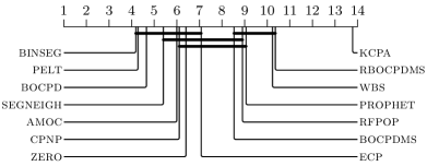
(b)

(c)

(d)

Figure 3: Critical-difference diagrams showing the mean rank of the methods for both experiments and both metrics on univariate time series. Methods that are not significantly different (at $\alpha=0.05$) are connected. Lower ranks are better.

While the average scores allow for general statements on the performance of the different methods, they are not suitable for evaluating the significance of performance differences because they represent measurements on distinct data sets (Demšar, 2006). Instead, an analysis of ranks can be used to show statistically significant differences. This involves assigning a numeric rank $R_{\ell,n}$ to method $\ell$ on data set $n$ with the best performing method receiving rank 1, the second best rank 2, etc. In the case of ties fractional ranks are assigned (i.e., if two methods achieve the highest score on a data set they are both assigned rank 1.5 and the third-best method is assigned rank 3). As discussed in detail in Demšar (2006), the Friedman test is a non-parametric test to evaluate the null hypothesis that all methods perform equally well. Furthermore, pairwise tests can be performed to assess whether two methods perform significantly differently, while correcting for the family-wise error rate.

Let $\bar{R}_{\ell}$ denote the average rank of method $\ell\in\{1,\ldots,L\}$ over all $N$ data sets. Under the null hypothesis of equal performance between the methods the Friedman test statistic, given by

$$\chi_{F}^{2}=\frac{12N}{L(L+1)}\left[\sum_{\ell=1}^{L}R_{\ell}^{2}-\frac{L(L+1)^{2}}{4}\right],$$ (7)

follows a $\chi^{2}$ distribution with $L-1$ degrees of freedom (Friedman, 1937, 1940). When running this test for the experiments on univariate data sets we reject the null hypothesis for both metrics on both experiments ($\chi^{2}\approx 200$ in all cases, resulting in $p$-values of zero). We can subsequently perform post-hoc tests to uncover statistically significant differences between methods. While Demšar (2006) recommends the Nemenyi test (Nemenyi, 1963) as a post-hoc test for individual differences, later work by Benavoli et al. (2016) argued that the Wilcoxon signed-rank test is to be preferred (Wilcoxon, 1945). Thus, for each pair of methods we compute the Wilcoxon signed-rank test with the null hypothesis of no significant differences in the performance of two methods. To correct for multiple testing we subsequently apply Holm’s procedure to control the family-wise error rate (Holm, 1979).

To summarize the results of the statistical tests we use the critical-difference (CD) diagrams proposed by Demšar (2006), see Figure 3. These figures show the average ranks of the methods, with methods that are not significantly different from each other connected by horizontal lines. For example, in Figure 3a the wbs and rfpop methods perform statistically significantly different from all other methods, but not from each other. The CD-diagram for the Oracle experiment also shows that when hyperparameters can be varied the bocpd method achieves the highest average rank. Moreover, depending on the metric considered it also statistically significantly outperforms a number of alternative methods (8 methods for the F1 score). It is noteworthy that even though bocpd assumes a simple Gaussian model with constant mean for each segment, it outperforms methods that allow for more complex time series behavior such as trend and seasonality (prophet), or autoregressive structures (bocpdms). From the critical difference diagrams we can also see that for both experiments and metrics, the kcpa, prophet, and wbs methods perform statistically significantly worse than the best performing methods. We also see that in our experiments no method performs significantly better than the zero method on the Default experiment, while this does not hold for the Oracle experiment.

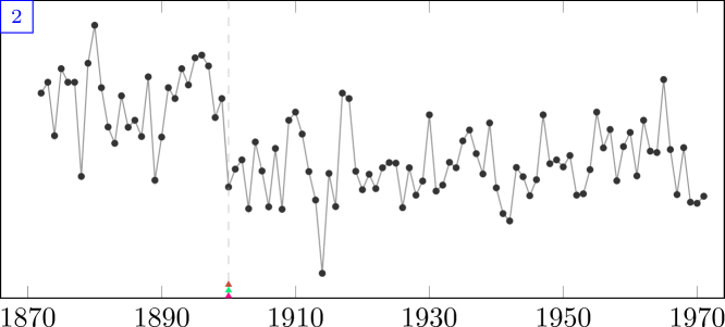
Figure 26: Yearly volume of the Nile river at Aswan. A dam was built in 1898. Data obtained from the website for the book by Durbin and Koopman (2012). This data set differs from the Nile data set for the period 622 to 1284 AD, used in other change point work.

By analyzing the performance of the methods on each individual time series in the data set we can gain some understanding of which time series are “easy”, in the sense that many methods achieve high scores on the evaluation metrics (see Appendix C). For the Default experiment, it is particularly noticeable that 9 of the 14 methods achieve an F1 score of 1.0 on the nile time series. One possible explanation for this could be that this series exhibits a single change point (according to most annotators, see Figure 26), which also appears to be a clear shift in the mean of the series. We can also look at which time series appeared to be “difficult”, in the sense that the methods failed to do well on it. Here, one noticeable case is the businv series where annotators generally agree on three change point locations, yet even in the Oracle experiment the maximum obtained F1 score is only 0.650.

Finally, we observe that the choice of evaluation metric affects the ranking of the algorithms (see Figure 3). Because the annotations are combined in a single set of ground truth change points when computing the precision, it is easier to achieve a high F1-score than it is to obtain a high score on the covering metric. Indeed, a high score on the covering metric indicates a high degree of agreement with each individual annotator, whereas a high value on the F1-score indicates a strong agreement with the combined set of annotations. Nevertheless, the best performing method is the same regardless of the metric, which reflects a degree of stability in the relative performance of the methods.

6 Discussion

We have introduced the first dedicated data set of human-annotated real-world time series from diverse application domains that is specifically designed for the evaluation and development of change point detection algorithms. Moreover, we have presented a framework for evaluating change point detection algorithms against ground truth provided by multiple human annotators, with two change point metrics that take distinct but complementary approaches to evaluating detection performance. With this data set we have conducted a thorough evaluation of a large selection of existing change point algorithms in an effort to discover those that perform best in practice. This benchmark study has shown that the binary segmentation algorithm of Scott and Knott (1974) performs best on univariate time series when using the default algorithm parameters from Killick and Eckley (2014), but its performance is not statistically significantly different from several other change point detection methods. When hyperparameter tuning is performed, the bocpd method of Adams and MacKay (2007) outperforms all other methods on both univariate and multivariate time series. However, the differences between it and some other algorithms (binseg, segneigh, and rfpop, among others) have been shown to not be statistically significantly different.

Both the introduced data set and the benchmark study can be extended and improved in the future, and our open-source code repository linked previously is set up to facilitate this. However, the present paper has already provided novel insights in the practical performance of change point detection algorithms and indicated potential topics for further research on algorithm development. For instance, future work could focus on incorporating automated hyperparameter tuning methods to bridge the gap between the Default and Oracle performance of the methods (perhaps taking inspiration from the work of Turner et al., 2009 for bocpd). It would also be relevant to understand why binseg performs as well or better than some of the more advanced methods, especially in the absence of hyperparameter tuning. Importantly, the presented change point data set and benchmark study motivate these research directions based on a quantitative analysis of algorithm performance, which was not previously possible.

Because of the unsupervised nature of the change point detection problem, it is difficult to compare algorithms in settings other than through simulation studies. But since the goal is ultimately to apply these algorithms to real-world time series, we should strive to ensure that they work well in practice. The change point data set presented here was inspired by the Berkeley Segmentation Data Set introduced in Martin et al. (2001) as well as the PASCAL VOC challenge (Everingham et al., 2010). In the past, these data sets have been crucial in accelerating the state of the art in image segmentation and object recognition, respectively. Our hope is that the data set and the benchmark study presented in this work can do the same for change point detection.

Changelog

Below is a list of changes to the arXiv version of this paper.

• v3

  • Expanded the grid search for some of the methods in the Oracle experiment

  • Changed from rank plots to critical-difference diagrams

  • Updated the results section taking into account the above changes

  • Expanded analysis of annotator agreement

  • Various minor corrections and clarifications

• v2

  • Added the zero method to the comparison.

  • Added summary statistics in the text regarding the length of the time series and the number of annotated change points.

  • Added rank plots for multivariate time series to the appendix.

  • Corrected an error in the computation of the F1 score and updated the results and the online code repository. This correction had no major effect on our conclusions.

  • Made minor revisions in Section 5.2 and Section 6 to reflect minor changes in the relative performance of the algorithms.

  • Updated acknowledgements.

• v1

  • Initial version.

Appendix A Simulation Details

This section presents additional details of the implementations and configurations used for each of the algorithms. Where possible, we used packages made available by the authors of the various methods. During the grid search those hyperparameter configurations that led to computational errors (e.g., numerical overflow) were skipped. While we describe our experimental setup in detail below, we also recommend the reader to check our online repository to reproduce our setup exactly.

• amoc, binseg, pelt, and segneigh were implemented using the R changepoint package, v2.2.2 (Killick and Eckley, 2014).

  • As default parameters we used the cpt.mean function, following Fryzlewicz (2014), with the Modified Bayes Information Criterion (MBIC) penalty, the Normal test statistic, and minimum segment length of 1. For binseg and segneigh we additionally used the default value of $5$ for the maximum number of change points/segments.

  • During the grid search, we varied the parameters as follows:

    Function:

    cpt.mean, cpt.var, and cpt.meanvar.

    Penalty:

    None, SIC, BIC, MBIC, AIC, Hannan-Quinn, Asymptotic (using p-value 0.05), and Manual (with a grid of 101 values for the regularization parameter, evenly spaced on a log scale between $10^{-3}$ and $10^{3}$).

    Test Statistic:

    Normal, CUSUM, CSS, Gamma, Exponential, and Poisson (where appropriate for the specified function).

    Max. CP:

    5 (default) or $T/2+1$ (max). Only for binseg or segneigh.

    Combinations of parameters that were invalid for the method were ignored.

• cpnp was implemented with the R changepoint.np package (v0.0.2). The penalty was varied in the same way as for pelt (see above) with the addition that in the grid search the number of quantiles was varied on the grid $\{10,20,30,40\}$.

• rfpop was called using the robseg package available on GitHub. As default setting the biweight loss function was used. During the grid search the parameters were varied as follows:

  Loss:

  L1, L2, Outlier, Huber

  Penalty value:

  lambda was varied on a grid of 101 values evenly spaced on a log scale between $10^{-3}$ and $10^{3}$ (as above for the methods in the changepoint package).

  Threshold:

  the lthreshold parameter was varied on a grid of 11 values evenly spaced on a log scale between $10^{-1}$ and $10^{1}$.

  We observe that because in addition to the loss function this method has two parameters that need to be evaluated on a grid, it has the largest number of hyperparameter configurations of any method in the Oracle experiment ($2,424$ in total).

• ecp and kcpa were accessed through the R ecp package (v3.1.1) available on CRAN (James and Matteson, 2013). For ecp the parameter settings were:

  • As default parameters we used the e.divisive function with $\alpha=1$, minimum segment size of 30, 199 runs for the permutation test and a significance level of 0.05.

  • The grid search consisted of:

    Algorithm:

    e.divisive or e.agglo

    Significance level:

    0.05 or 0.01.

    Minimum segment size:

    2 (minimal) or 30 (default)

    $\alpha$

    : $(0.5,1.0,1.5)$

    For the e.agglo algorithm only the $\alpha$ parameter has an effect.

  The kcpa method takes two parameters: a cost and a maximum number of change points. In the default experiment the cost parameter was set to 1 and we allowed the maximum number of change points possible. In the grid search the cost parameter was varied in the same way as above for the methods in the changepoint package, on a grid of 101 values evenly spaced on a log scale between $10^{-3}$ and $10^{3}$, and the maximum number of change points was varied between the maximum possible and $5$, which corresponds to the methods in the changepoint package.

• wbs was evaluated using the R package of the same name available on CRAN (v1.4).

  • As defaults we used the SSIC penalty, the integrated version, and the default of 50 for the maximum number of change points.

  • During the grid search we used:

    Penalty:

    SSIC, BIC, MBIC

    Integrated:

    true, false

    Max CP:

    50 (default) or $T$ (max)

• bocpd was called using the R package ocp (v0.1.1), available on CRAN (Pagotto, 2019). For the experiments we used the Gaussian distribution with the negative inverse gamma prior. The prior mean was set to $0$, since the data is standardized. No truncation of the run lengths was applied.

  • For the default experiment the intensity ($\lambda_{\text{gap}}$) was set to 100, the prior variables were set to $\alpha_{0}=1$, $\beta_{0}=1$, and $\kappa_{0}=1$.

  • For the grid search, we varied the parameters as follows:

    Intensity:

    $(10,50,100,200)$

    $\alpha_{0}$:

    $(0.01,0.1,1,10,100)$

    $\beta_{0}$:

    $(0.01,0.1,1,10,100)$

    $\kappa_{0}$:

    $(0.01,0.1,1,10,100)$

• bocpdms and rbocpdms were run with the code available on GitHub. The settings for bocpdms were the same as that for bocpd above, with the exception that during the grid search run length pruning was applied by keeping the best 100 run lengths. This was done for speed considerations. No run length pruning was needed for bocpdms with the default configuration, but this was applied for rbocpdms. For rbocpdms we used the same settings, but supplied additional configurations for the $\alpha_{0}$ and $\alpha_{\text{rld}}$ parameters. As default values and during the grid search we used $\alpha_{0}=\alpha_{\text{rld}}=0.5$. For both methods we applied a timeout of 30 minutes during the grid search and we used a timeout of 4 hours for rbocpdms in the default experiment.

• prophet was run in R using the prophet package (v0.4). As Prophet requires the input time vector to be a vector of dates or datetimes, we supplied this where available and considered the series that did not have date information to be a daily series. By supplying the dates of the observations Prophet automatically chooses whether to include various seasonality terms. For both experiments we allowed detecting of change points on the entire input range and used a threshold of $0.01$ for selecting the change points (in line with the change point plot function in the Prophet package). During the grid search we only varied the maximum number of change points between the default (25) and the theoretical maximum ($T$).

Appendix B Simulated Annotator Agreement

In this section we present the results of a simulation study that aims to quantify the extent to which the annotator agreement described in Section 4.4 can be expected by chance.

For every time series in the data set we simulate a set of change point annotations for each of the $K=5$ annotators. Next, for each annotator we compute the one-vs-rest (OvR) annotator agreement compared to the simulated other annotators, as described in the main text. These values are then averaged into a single value that represents the simulated average OvR annotator agreement. By repeating this process a large number of times we obtain a distribution over the average OvR annotator agreement for a particular time series. Naturally, we can also compute the average OvR annotator agreement for the human annotators. We can then compute the $p$-value for the hypothesis that the average OvR annotator agreement for the human annotators is larger than what is expected by chance. Formally, if $X$ is a random variable reflecting the distribution of the simulated average OvR annotator agreement and $\bar{x}$ is the observed human OvR annotator agreement, then we are interested in the probability $p(X\geq\bar{x})$.

Recall from the main text that $n_{k}$ is the number of change points identified by annotator $k$, and $\tau_{i}$ is the index of change point $i\in\{1,\ldots,n_{k}\}$. We simulate the annotations as follows for each simulated annotator $k\in\{1,\ldots,K\}$,

$$n_{k} \sim\text{Pois}(\eta)$$ (8)

$$\tau_{i} \sim\text{Unif}(2,T-1),\qquad\forall i\in\{1,\ldots,n_{k}\},$$ (9)

where $\eta$ is a hyperparameter for the simulation discussed below. Note that the domain for the change points $\tau_{i}$ is chosen such that no change points can be declared at the first and last time index. For each time series in the data set we simulate 100,000 sets of annotations and compute the average OvR annotator agreement. The $p$-value for each series is then approximated as the proportion of realizations of $X$ that are larger or equal to $\bar{x}$. The rate of the Poisson distribution, $\eta$, affects the number of change points for each simulated annotator. A priori, there is no information on how this rate should be chosen such that the simulation is as close as possible to the real-world case. Thus, we propose to set $\eta$ to the number of change points declared per human annotator averaged over all time series in the data set ($\eta\approx 2.295$).

Dataset	Covering	F1
apple	0.014	0.001
bank	0.000	0.000
bee_waggle_6	0.001	0.000
bitcoin	0.008	0.049
brent_spot	0.149	0.018
businv	0.011	0.000
centralia	0.172	0.744
children_per_woman	0.000	0.000
co2_canada	0.013	0.000
construction	0.016	0.008
debt_ireland	0.000	0.001
gdp_argentina	0.042	0.001
gdp_croatia	0.006	0.013
gdp_iran	0.015	0.006
gdp_japan	0.009	0.000
global_co2	0.051	0.000
homeruns	0.606	0.043
iceland_tourism	0.000	0.000
jfk_passengers	0.004	0.003
lga_passengers	0.275	0.003
measles	0.000	0.000
nile	0.002	0.000
occupancy	0.416	0.001
ozone	0.009	0.001
quality_control_1	0.000	0.000
quality_control_2	0.001	0.000
quality_control_3	0.000	0.000
quality_control_4	0.145	0.001
quality_control_5	0.000	0.000
rail_lines	0.002	0.001
ratner_stock	0.000	0.012
robocalls	0.019	0.018
run_log	0.052	0.001
scanline_126007	0.735	0.014
scanline_42049	0.002	0.000
seatbelts	0.005	0.000
shanghai_license	0.000	0.000
uk_coal_employ	0.389	0.002
unemployment_nl	0.718	0.005
us_population	0.011	0.000
usd_isk	0.001	0.003
well_log	0.005	0.001

Table 3: Simulated $p$-values for the average one-vs-rest annotator agreement observed for the human annotators. Values larger than a significance level of $0.05$ are highlighted in bold.

Using the above simulation setup we obtain the $p$-values listed in Table 3. We observe that conditional on the assumptions made in the simulation, for most time series in the data set the observed average OvR annotator agreement for the human annotators is significantly larger than what can be expected by chance. For the F1-score we find a $p$-value larger than $0.05$ only for the centralia time series. This is unsurprising for two reasons: this series consists of only 15 observations, and there is disagreement amongst the annotators on the existence of change points in the series. For the covering metric there are few additional series where the $p$-value obtained from the simulation is larger than $0.05$. This can be explained by the fact that this metric rewards high agreement with each individual annotator, and in these series there is some amount of disagreement among the annotators.

Appendix C Additional Tables and Figures

Below we present additional tables and figures to support the material in the main text. In some tables the results on the quality control time series are included for completeness, but these are not used in the benchmark study.

C.1 Tables

Table 4: Descriptive statistics of the time series included in the data set. The three rightmost columns respectively show the minimum, maximum, and average number of change points marked by the annotators (see Section D for the complete annotations). The series marked with a dagger ($\dagger$) are financial time series that only yield observations on trading days, which were additionally sampled every three days to reduce their length.

	Frequency	Length ($T$)	Dim. ($d$)	Min CP	Max CP	Avg CP
1. apple	Daily†	622	2	1	8	2.4
2. bank	Daily	581	1	0	0	0.0
3. bee_waggle_6	Unit	609	4	0	2	0.4
4. bitcoin	Daily†	774	1	1	7	4.0
5. brent_spot	Fortnightly	500	1	2	11	6.0
6. businv	Monthly	330	1	0	3	2.2
7. centralia	Decenially	15	1	0	3	1.2
8. children_per_woman	Yearly	301	1	1	4	2.2
9. co2_canada	Yearly	215	1	2	7	4.4
10. construction	Monthly	319	1	0	2	1.2
11. debt_ireland	Yearly	21	1	2	4	2.4
12. gdp_argentina	Yearly	59	1	0	3	1.2
13. gdp_croatia	Yearly	24	1	0	1	0.6
14. gdp_iran	Yearly	58	1	0	3	1.6
15. gdp_japan	Yearly	58	1	0	1	0.4
16. global_co2	Quadrennial	104	1	0	2	0.8
17. homeruns	Yearly	118	1	0	7	2.2
18. iceland_tourism	Monthly	199	1	0	1	0.2
19. jfk_passengers	Monthly	468	1	0	2	1.0
20. lga_passengers	Monthly	468	1	0	7	3.4
21. measles	Weekly	991	1	0	1	0.2
22. nile	Yearly	100	1	0	1	0.6
23. occupancy	Every 16 min.	509	4	2	12	6.2
24. ozone	Yearly	54	1	0	2	1.0
25. quality_control_1	Unit	313	1	1	1	1.0
26. quality_control_2	Unit	283	1	0	1	0.8
27. quality_control_3	Unit	366	1	1	1	1.0
28. quality_control_4	Unit	500	1	0	4	1.2
29. quality_control_5	Unit	325	1	0	0	0.0
30. rail_lines	Yearly	37	1	1	2	1.8
31. ratner_stock	Daily†	600	1	1	2	1.6
32. robocalls	Monthly	52	1	0	2	1.6
33. run_log	Every 5 sec.	376	2	0	9	6.6
34. scanline_126007	Unit	481	1	0	22	5.2
35. scanline_42049	Unit	481	1	2	10	6.6
36. seatbelts	Monthly	192	1	0	3	1.8
37. shanghai_license	Monthly	205	1	1	2	1.2
38. uk_coal_employ	Yearly	105	1	0	6	3.8
39. unemployment_nl	Yearly	214	1	0	9	4.0
40. us_population	Monthly	816	1	0	1	0.4
41. usd_isk	Monthly	247	1	1	4	2.4
42. well_log	Unit	675	1	2	17	9.6

Table 5: Default-Covering. Results for each method on each of the time series for the experiment with default settings using the covering metric. Values are unavailable either due to a failure (F), because of missing values in the series unsupported by the method (M), or because the method is not suited for multidimensional series (blank). Highest values for each time series are shown in bold.

Dataset	amoc	binseg	bocpd	bocpdms	cpnp	ecp	kcpa	pelt	prophet	rbocpdms	rfpop	segneigh	wbs	zero
bank	0.967	0.509	0.048	0.188	0.053	0.127	0.036	0.509	0.361	0.644	0.036	0.509	0.048	1.000
bitcoin	0.764	0.754	0.717	0.748	0.364	0.209	0.046	0.758	0.723	F	0.168	0.758	0.304	0.516
brent_spot	0.423	0.627	0.586	0.265	0.411	0.387	0.022	0.627	0.527	0.504	0.225	0.630	0.242	0.266
businv	0.574	0.562	0.463	0.459	0.402	0.311	0.013	0.603	0.478	0.529	0.123	0.494	0.108	0.461
centralia	0.675	0.564	0.612	0.650	0.564	0.675	0.440	0.564	0.675	0.624	0.528	0.564	0.253	0.675
children_per_woman	0.798	0.798	0.758	0.427	0.486	0.397	0.048	0.798	0.521	0.762	0.154	0.771	0.186	0.429
co2_canada	0.527	0.608	0.716	0.276	0.514	0.639	0.263	0.611	0.540	0.432	0.497	0.612	0.480	0.278
construction	0.525	0.466	0.395	0.571	0.334	0.352	0.016	0.423	0.502	0.584	0.092	0.423	0.198	0.575
debt_ireland	0.321	0.635	0.584	0.312	0.635	0.321	0.210	0.635	0.321	0.306	0.489	0.635	0.248	0.321
gdp_argentina	0.667	0.667	0.630	0.711	0.451	0.737	0.061	0.667	0.534	0.711	0.332	0.631	0.068	0.737
gdp_croatia	0.605	0.605	0.642	0.655	0.642	0.708	0.108	0.605	0.708	0.655	0.353	0.605	0.108	0.708
gdp_iran	0.484	0.477	0.520	0.580	0.448	0.583	0.062	0.477	0.583	0.580	0.248	0.503	0.066	0.583
gdp_japan	0.654	0.654	0.578	0.645	0.522	0.802	0.041	0.654	0.802	0.777	0.269	0.654	0.048	0.802
global_co2	0.743	0.748	0.640	0.731	0.313	0.535	0.173	0.638	0.284	0.745	0.368	0.634	0.187	0.758
homeruns	0.683	0.683	0.526	0.677	0.516	0.611	0.047	0.683	0.574	0.559	0.354	0.590	0.312	0.511
iceland_tourism	0.764	0.764	0.595	0.616	0.383	0.382	0.017	0.764	0.453	0.869	0.293	0.650	0.512	0.946
jfk_passengers	0.839	0.839	0.541	0.831	0.561	0.438	0.008	0.839	0.373	0.668	0.264	0.791	0.409	0.630
lga_passengers	0.427	0.458	0.496	0.444	0.473	0.386	0.013	0.474	0.434	0.382	0.412	0.543	0.477	0.383
measles	0.951	0.951	0.081	0.255	0.098	0.060	0.005	0.213	0.603	0.296	0.046	0.367	0.081	0.951
nile	0.880	0.880	0.888	0.870	0.880	0.857	0.032	0.880	0.758	0.753	0.880	0.880	0.880	0.758
ozone	0.701	0.600	0.602	0.560	0.441	0.574	0.070	0.635	0.574	0.614	0.309	0.627	0.070	0.574
rail_lines	0.786	0.786	0.767	0.416	0.738	0.428	0.103	0.786	0.534	0.416	0.439	0.786	0.103	0.428
ratner_stock	0.873	0.913	0.796	0.866	0.380	0.185	0.021	0.908	0.444	0.864	0.162	0.914	0.176	0.450
robocalls	0.641	0.641	0.808	0.622	0.677	0.601	0.069	0.641	0.601	0.607	0.447	0.760	0.069	0.601
scanline_126007	0.519	0.464	0.346	0.506	0.433	0.327	0.025	0.444	0.503	F	0.316	0.567	0.263	0.503
scanline_42049	0.424	0.631	0.892	0.832	0.529	0.490	0.121	0.745	0.441	0.418	0.257	0.730	0.432	0.211
seatbelts	0.683	0.797	0.757	0.526	0.750	0.615	0.020	0.797	0.628	0.526	0.484	0.765	0.727	0.528
shanghai_license	0.920	0.920	0.856	0.616	0.474	0.518	0.020	0.920	0.768	0.730	0.381	0.826	0.209	0.547
uk_coal_employ	M	M	M	0.429	M	0.356	0.356	M	0.481	M	M	M	M	0.356
unemployment_nl	0.507	0.669	0.495	0.570	0.503	0.470	0.039	0.648	0.507	0.539	0.243	0.648	0.222	0.507
us_population	0.736	0.391	0.219	0.801	0.391	0.089	0.003	0.506	0.096	0.632	0.803	0.307	0.043	0.803
usd_isk	0.853	0.735	0.672	0.866	0.480	0.616	0.023	0.730	0.436	0.578	0.163	0.730	0.194	0.436
well_log	0.453	0.695	0.776	0.787	0.772	0.601	0.020	0.679	0.411	0.661	0.787	0.647	0.719	0.225
quality_control_1	0.992	0.992	0.887	0.990	0.683	0.620	0.010	0.992	0.693	0.986	0.655	0.992	0.687	0.503
quality_control_2	0.922	0.922	0.927	0.921	0.922	0.927	0.010	0.922	0.723	0.922	0.922	0.922	0.922	0.638
quality_control_3	0.996	0.996	0.997	0.977	0.831	0.997	0.008	0.996	0.500	0.990	0.658	0.996	0.996	0.500
quality_control_4	0.563	0.518	0.511	0.670	0.481	0.257	0.009	0.538	0.508	0.733	0.059	0.538	0.080	0.673
quality_control_5	1.000	1.000	1.000	0.994	1.000	1.000	0.006	1.000	1.000	0.994	1.000	1.000	1.000	1.000
apple			0.365	0.359		0.305	0.007			0.694				0.425
bee_waggle_6			0.089	0.860		0.116	0.004			0.226				0.891
occupancy			0.549	0.443		0.530	0.050			0.437				0.236
run_log			0.815	0.387		0.657	0.128			0.584				0.304

Table 6: Default-F1. Results for each method on each of the time series for the experiment with default settings using the F1-score. Values are unavailable either due to a failure (F), because of missing values in the series unsupported by the method (M), or because the method is not suited for multidimensional series (blank). Highest values for each time series are shown in bold.

Dataset	amoc	binseg	bocpd	bocpdms	cpnp	ecp	kcpa	pelt	prophet	rbocpdms	rfpop	segneigh	wbs	zero
bank	0.667	0.400	0.047	0.118	0.044	0.154	0.008	0.400	0.154	0.286	0.015	0.333	0.039	1.000
bitcoin	0.367	0.426	0.692	0.269	0.463	0.338	0.092	0.672	0.446	F	0.284	0.672	0.464	0.450
brent_spot	0.272	0.483	0.521	0.239	0.607	0.478	0.104	0.465	0.249	0.321	0.490	0.431	0.516	0.315
businv	0.455	0.370	0.270	0.370	0.304	0.301	0.047	0.370	0.275	0.238	0.245	0.312	0.230	0.588
centralia	0.763	0.909	0.909	0.846	0.909	0.763	0.714	0.909	0.763	0.846	1.000	0.909	0.556	0.763
children_per_woman	0.618	0.618	0.637	0.337	0.326	0.349	0.068	0.618	0.310	0.432	0.246	0.337	0.271	0.507
co2_canada	0.544	0.691	0.619	0.265	0.578	0.817	0.169	0.661	0.482	0.381	0.569	0.661	0.520	0.361
construction	0.516	0.709	0.634	0.410	0.602	0.574	0.038	0.709	0.324	0.291	0.185	0.709	0.316	0.696
debt_ireland	0.469	0.760	0.760	0.611	0.760	0.469	0.519	0.760	0.469	0.530	0.824	0.760	0.538	0.469
gdp_argentina	0.889	0.889	0.947	0.583	0.818	0.824	0.131	0.889	0.615	0.452	0.571	0.947	0.148	0.824
gdp_croatia	0.583	0.583	1.000	0.583	1.000	0.824	0.160	0.583	0.824	0.452	0.400	0.583	0.167	0.824
gdp_iran	0.492	0.492	0.622	0.492	0.330	0.652	0.219	0.492	0.652	0.395	0.609	0.395	0.246	0.652
gdp_japan	0.615	0.615	0.800	0.471	0.667	0.889	0.068	0.615	0.889	0.471	0.190	0.615	0.077	0.889
global_co2	0.929	0.929	0.754	0.458	0.421	0.754	0.167	0.754	0.463	0.458	0.293	0.754	0.179	0.846
homeruns	0.812	0.812	0.729	0.552	0.604	0.675	0.133	0.812	0.723	0.508	0.661	0.397	0.593	0.659
iceland_tourism	0.643	0.643	0.486	0.391	0.391	0.391	0.021	0.643	0.220	0.667	0.200	0.486	0.200	0.947
jfk_passengers	0.776	0.776	0.437	0.559	0.574	0.437	0.026	0.776	0.354	0.296	0.344	0.650	0.437	0.723
lga_passengers	0.422	0.438	0.630	0.297	0.606	0.392	0.054	0.438	0.366	0.348	0.498	0.395	0.524	0.535
measles	0.947	0.947	0.069	0.124	0.118	0.069	0.004	0.124	0.391	0.117	0.030	0.327	0.039	0.947
nile	1.000	1.000	1.000	0.800	1.000	1.000	0.040	1.000	0.824	0.452	1.000	1.000	1.000	0.824
ozone	0.531	0.650	0.650	0.531	0.750	0.723	0.109	1.000	0.723	0.559	0.375	1.000	0.113	0.723
rail_lines	0.846	0.846	0.846	0.349	0.966	0.537	0.200	0.846	0.423	0.349	0.571	0.846	0.205	0.537
ratner_stock	0.776	0.824	0.783	0.500	0.306	0.282	0.034	0.650	0.280	0.559	0.203	0.824	0.250	0.571
robocalls	0.800	0.800	0.966	0.696	0.832	0.636	0.179	0.800	0.636	0.593	0.714	0.966	0.182	0.636
scanline_126007	0.710	0.739	0.820	0.718	0.889	0.732	0.101	0.759	0.644	F	0.649	0.732	0.616	0.644
scanline_42049	0.485	0.713	0.962	0.844	0.705	0.580	0.164	0.804	0.269	0.390	0.460	0.748	0.571	0.276
seatbelts	0.474	0.683	0.583	0.383	0.509	0.321	0.051	0.683	0.452	0.383	0.494	0.583	0.583	0.621
shanghai_license	0.868	0.868	0.713	0.491	0.437	0.698	0.048	0.868	0.532	0.326	0.357	0.713	0.208	0.636
uk_coal_employ	M	M	M	0.495	M	0.513	0.513	M	0.639	M	M	M	M	0.513
unemployment_nl	0.566	0.876	0.683	0.592	0.683	0.620	0.145	0.773	0.566	0.495	0.549	0.773	0.571	0.566
us_population	1.000	0.667	0.216	0.471	0.216	0.174	0.007	0.471	0.159	0.320	0.889	0.320	0.077	0.889
usd_isk	0.785	0.657	0.609	0.678	0.504	0.661	0.079	0.657	0.489	0.282	0.390	0.657	0.513	0.489
well_log	0.279	0.534	0.796	0.797	0.822	0.818	0.069	0.555	0.149	0.517	0.923	0.485	0.724	0.237
quality_control_1	1.000	1.000	0.800	0.667	0.667	0.667	0.025	1.000	0.500	0.667	0.667	1.000	0.571	0.667
quality_control_2	1.000	1.000	1.000	0.667	1.000	1.000	0.028	1.000	0.545	0.667	1.000	1.000	1.000	0.750
quality_control_3	1.000	1.000	1.000	0.667	0.571	1.000	0.022	1.000	0.667	0.667	0.286	1.000	1.000	0.667
quality_control_4	0.810	0.873	0.658	0.438	0.608	0.393	0.028	0.726	0.335	0.360	0.233	0.726	0.246	0.780
quality_control_5	1.000	1.000	1.000	0.500	1.000	1.000	0.006	1.000	1.000	0.500	1.000	1.000	1.000	1.000
apple			0.513	0.382		0.513	0.029			0.239				0.594
bee_waggle_6			0.121	0.388		0.124	0.010			0.179				0.929
occupancy			0.807	0.461		0.750	0.107			0.329				0.341
run_log			1.000	0.475		0.792	0.139			0.660				0.446

Table 7: Oracle-Covering. Maximum segmentation covering score for each method on each of the time series after running the grid search. Values are unavailable either due to a failure (F), because of missing values in the series unsupported by the method (M), the method timing out (T), or because the method is not suited for multidimensional series (blank). Highest values for each time series are shown in bold.

Dataset	amoc	binseg	bocpd	bocpdms	cpnp	ecp	kcpa	pelt	prophet	rbocpdms	rfpop	segneigh	wbs	zero
bank	1.000	1.000	1.000	0.997	1.000	0.238	0.509	1.000	1.000	0.997	1.000	1.000	0.053	1.000
bitcoin	0.771	0.771	0.822	0.778	0.757	0.772	0.778	0.796	0.723	0.743	0.802	0.796	0.409	0.516
brent_spot	0.503	0.650	0.667	0.484	0.642	0.653	0.571	0.659	0.527	0.709	0.669	0.659	0.310	0.266
businv	0.574	0.580	0.693	0.459	0.676	0.690	0.405	0.705	0.539	0.689	0.603	0.705	0.154	0.461
centralia	0.675	0.675	0.753	0.650	0.675	0.753	0.753	0.675	0.675	0.624	0.675	0.675	0.253	0.675
children_per_woman	0.804	0.804	0.834	0.925	0.817	0.718	0.613	0.804	0.521	0.839	0.798	0.804	0.284	0.429
co2_canada	0.527	0.776	0.773	0.584	0.667	0.751	0.739	0.760	0.605	0.654	0.768	0.760	0.552	0.278
construction	0.629	0.626	0.631	0.571	0.575	0.524	0.395	0.575	0.561	0.744	0.732	0.626	0.300	0.575
debt_ireland	0.635	0.859	0.814	0.803	0.777	0.798	0.747	0.779	0.321	0.689	0.859	0.859	0.248	0.321
gdp_argentina	0.737	0.737	0.737	0.711	0.737	0.737	0.367	0.737	0.592	0.711	0.737	0.737	0.326	0.737
gdp_croatia	0.708	0.708	0.708	0.675	0.708	0.708	0.623	0.708	0.708	0.708	0.783	0.708	0.108	0.708
gdp_iran	0.583	0.583	0.583	0.719	0.583	0.583	0.505	0.583	0.583	0.753	0.626	0.583	0.295	0.583
gdp_japan	0.802	0.802	0.802	0.777	0.802	0.802	0.525	0.802	0.802	0.802	0.802	0.802	0.283	0.802
global_co2	0.758	0.758	0.758	0.745	0.758	0.665	0.602	0.758	0.284	0.745	0.758	0.758	0.338	0.758
homeruns	0.694	0.694	0.694	0.681	0.646	0.694	0.501	0.694	0.575	0.688	0.687	0.694	0.407	0.511
iceland_tourism	0.946	0.946	0.946	0.936	0.946	0.842	0.655	0.946	0.498	0.936	0.946	0.946	0.512	0.946
jfk_passengers	0.844	0.845	0.842	0.855	0.845	0.807	0.563	0.839	0.373	0.627	0.859	0.845	0.514	0.630
lga_passengers	0.434	0.541	0.563	0.512	0.534	0.653	0.536	0.547	0.446	0.470	0.547	0.547	0.501	0.383
measles	0.951	0.951	0.951	0.950	0.951	0.105	0.400	0.951	0.603	0.096	0.951	0.951	0.084	0.951
nile	0.888	0.880	0.888	0.876	0.880	0.888	0.888	0.880	0.758	0.876	0.888	0.880	0.880	0.758
ozone	0.721	0.701	0.741	0.798	0.648	0.676	0.451	0.701	0.574	0.798	0.783	0.701	0.309	0.574
rail_lines	0.786	0.786	0.789	0.767	0.803	0.768	0.773	0.786	0.534	0.789	0.786	0.786	0.103	0.428
ratner_stock	0.874	0.915	0.908	0.872	0.892	0.874	0.771	0.914	0.444	0.863	0.914	0.914	0.182	0.450
robocalls	0.666	0.788	0.808	0.741	0.806	0.808	0.808	0.760	0.601	0.672	0.789	0.760	0.559	0.601
scanline_126007	0.634	0.633	0.631	0.688	0.561	0.390	0.494	0.633	0.503	0.581	0.578	0.633	0.329	0.503
scanline_42049	0.425	0.868	0.892	0.887	0.787	0.862	0.860	0.862	0.441	0.667	0.866	0.870	0.690	0.211
seatbelts	0.683	0.797	0.800	0.630	0.825	0.800	0.800	0.797	0.635	0.658	0.797	0.797	0.727	0.528
shanghai_license	0.930	0.930	0.929	0.911	0.929	0.920	0.497	0.930	0.804	0.912	0.924	0.930	0.351	0.547
uk_coal_employ	M	M	M	0.504	M	0.356	0.356	M	0.481	M	M	M	M	0.356
unemployment_nl	0.627	0.669	0.673	0.656	0.652	0.501	0.476	0.650	0.507	0.634	0.650	0.650	0.447	0.507
us_population	0.803	0.803	0.737	0.802	0.734	0.508	0.272	0.803	0.135	0.713	0.803	0.803	0.050	0.803
usd_isk	0.865	0.865	0.875	0.869	0.853	0.858	0.714	0.865	0.436	0.818	0.865	0.865	0.401	0.436
well_log	0.463	0.830	0.803	0.797	0.825	0.846	0.864	0.814	0.411	0.753	0.846	0.814	0.768	0.225
quality_control_1	0.996	0.992	0.996	0.990	0.992	0.989	0.620	0.992	0.693	0.990	0.992	0.992	0.687	0.503
quality_control_2	0.927	0.927	0.927	0.922	0.922	0.927	0.927	0.922	0.723	0.922	0.922	0.927	0.922	0.638
quality_control_3	0.997	0.996	0.997	0.991	0.996	0.997	0.997	0.996	0.500	0.991	0.996	0.996	0.996	0.500
quality_control_4	0.742	0.673	0.673	0.670	0.673	0.540	0.535	0.673	0.673	0.670	0.673	0.673	0.506	0.673
quality_control_5	1.000	1.000	1.000	0.994	1.000	1.000	1.000	1.000	1.000	0.994	1.000	1.000	1.000	1.000
apple			0.846	0.783		0.758	0.462			0.699				0.425
bee_waggle_6			0.891	0.887		0.116	0.730			0.737				0.891
occupancy			0.645	0.524		0.666	0.581			0.544				0.236
run_log			0.824	0.563		0.819	0.824			0.616				0.304

Table 8: Oracle-F1. Maximum F1-score for each method on each of the time series after running the grid search. Values are unavailable either due to a failure (F), because of missing values in the series unsupported by the method (M), the method timing out (T), or because the method is not suited for multidimensional series (blank). Highest values for each time series are shown in bold.

Dataset	amoc	binseg	bocpd	bocpdms	cpnp	ecp	kcpa	pelt	prophet	rbocpdms	rfpop	segneigh	wbs	zero
bank	1.000	1.000	1.000	0.500	1.000	0.200	0.333	1.000	1.000	0.500	1.000	1.000	0.043	1.000
bitcoin	0.507	0.780	0.733	0.533	0.611	0.625	0.665	0.783	0.446	0.422	0.727	0.783	0.690	0.450
brent_spot	0.465	0.670	0.631	0.309	0.735	0.636	0.553	0.641	0.249	0.621	0.641	0.651	0.564	0.315
businv	0.588	0.588	0.650	0.455	0.588	0.370	0.294	0.588	0.275	0.553	0.588	0.588	0.289	0.588
centralia	0.909	1.000	1.000	1.000	1.000	0.909	1.000	1.000	0.763	0.974	1.000	1.000	0.556	0.763
children_per_woman	0.678	0.678	0.787	0.826	0.734	0.551	0.525	0.778	0.310	0.580	0.637	0.778	0.500	0.507
co2_canada	0.544	0.893	0.924	0.479	0.677	0.875	0.867	0.894	0.482	0.621	0.894	0.894	0.681	0.361
construction	0.696	0.709	0.709	0.516	0.709	0.709	0.634	0.709	0.324	0.615	0.709	0.709	0.523	0.696
debt_ireland	0.760	1.000	1.000	0.892	0.958	0.980	1.000	1.000	0.469	0.958	1.000	1.000	0.538	0.469
gdp_argentina	0.889	0.947	0.947	0.583	0.889	0.889	0.800	0.947	0.615	0.818	0.947	0.947	0.421	0.824
gdp_croatia	1.000	0.824	1.000	0.583	1.000	0.824	0.800	0.824	0.824	0.824	1.000	0.824	0.167	0.824
gdp_iran	0.696	0.696	0.862	0.838	0.667	0.824	0.734	0.808	0.652	0.899	0.833	0.808	0.576	0.652
gdp_japan	1.000	1.000	1.000	0.615	1.000	1.000	0.500	1.000	0.889	1.000	1.000	1.000	0.222	0.889
global_co2	0.929	0.929	0.929	0.458	0.846	0.929	0.750	0.929	0.463	0.634	0.929	0.929	0.250	0.846
homeruns	0.812	0.889	0.829	0.675	0.681	0.829	0.829	0.873	0.723	0.879	0.961	0.873	0.664	0.659
iceland_tourism	0.947	0.947	0.947	0.486	0.947	1.000	0.486	0.947	0.220	0.667	0.947	0.947	0.200	0.947
jfk_passengers	0.776	0.776	0.776	0.650	0.776	0.651	0.651	0.776	0.354	0.420	0.776	0.776	0.437	0.723
lga_passengers	0.561	0.620	0.715	0.563	0.634	0.892	0.598	0.602	0.366	0.561	0.666	0.620	0.674	0.535
measles	0.947	0.947	0.947	0.486	0.947	0.080	0.281	0.947	0.391	0.090	0.947	0.947	0.041	0.947
nile	1.000	1.000	1.000	0.800	1.000	1.000	1.000	1.000	0.824	0.800	1.000	1.000	1.000	0.824
ozone	0.776	1.000	0.966	0.778	1.000	1.000	0.667	1.000	0.723	1.000	1.000	1.000	0.286	0.723
rail_lines	0.846	0.966	0.966	0.889	0.966	0.966	0.800	0.846	0.537	0.730	0.889	0.966	0.205	0.537
ratner_stock	0.776	0.832	0.929	0.559	0.776	0.776	0.754	0.824	0.280	0.686	0.824	0.824	0.378	0.571
robocalls	0.800	0.966	0.966	0.750	0.966	0.966	0.966	0.966	0.636	0.765	0.966	0.966	0.714	0.636
scanline_126007	0.710	0.920	0.964	0.837	0.927	0.870	0.838	0.889	0.644	0.570	0.914	0.940	0.818	0.644
scanline_42049	0.485	0.931	0.962	0.921	0.809	0.910	0.908	0.910	0.269	0.526	0.910	0.920	0.650	0.276
seatbelts	0.824	0.838	0.683	0.583	0.838	0.683	0.683	0.683	0.452	0.621	0.683	0.838	0.583	0.621
shanghai_license	0.966	0.966	0.868	0.651	0.966	0.868	0.465	0.966	0.532	0.778	0.966	0.966	0.385	0.636
uk_coal_employ	M	M	M	0.617	M	0.513	0.513	M	0.639	M	M	M	M	0.513
unemployment_nl	0.742	0.889	0.876	0.797	0.773	0.755	0.744	0.816	0.566	0.697	0.851	0.816	0.801	0.566
us_population	1.000	1.000	1.000	0.615	0.947	0.471	0.276	1.000	0.159	0.320	0.889	1.000	0.113	0.889
usd_isk	0.785	0.785	0.876	0.678	0.785	0.785	0.601	0.785	0.489	0.881	0.785	0.785	0.636	0.489
well_log	0.336	0.944	0.908	0.796	0.878	0.928	0.950	0.912	0.149	0.644	0.966	0.912	0.832	0.237
quality_control_1	1.000	1.000	1.000	0.667	1.000	1.000	0.667	1.000	0.500	0.667	1.000	1.000	0.667	0.667
quality_control_2	1.000	1.000	1.000	0.800	1.000	1.000	1.000	1.000	0.750	0.667	1.000	1.000	1.000	0.750
quality_control_3	1.000	1.000	1.000	0.766	1.000	1.000	1.000	1.000	0.667	0.667	1.000	1.000	1.000	0.667
quality_control_4	0.810	0.873	0.810	0.561	0.810	0.726	0.658	0.810	0.780	0.438	0.873	0.810	0.608	0.780
quality_control_5	1.000	1.000	1.000	0.500	1.000	1.000	1.000	1.000	1.000	0.500	1.000	1.000	1.000	1.000
apple			0.916	0.552		0.745	0.634			0.575				0.594
bee_waggle_6			0.929	0.651		0.233	0.651			0.359				0.929
occupancy			0.919	0.714		0.932	0.812			0.605				0.341
run_log			1.000	0.698		0.990	1.000			0.698				0.446

C.2 Multivariate Critical Difference Diagrams

(a)

(b)

(c)

(d)

Figure 4: Critical difference diagrams for both experiments and both metrics for the multivariate time series. Methods that are not significantly different (at $\alpha~{}=~{}0.05$) are connected. Lower ranks are better.

Appendix D Data Set Overview

In the following pages we show the time series included in the change point data set, as well as the provided annotations. Annotations are marked on the graphs by a dashed vertical line with one or more triangles on the horizontal axis that correspond to the number of annotators that marked that point as a change point. The colors of the triangles correspond to each of the five annotators for the time series. The number in the box on the left side of the figure is the number of annotators who believed there were no change points in the time series. A brief description including the source of the series is provided.

D.1 Real Time Series

This section lists the real time series from various sources and application domains.

[capbesideposition=left,top,capbesidewidth=5cm]figure[9cm]apple

Figure 5: The daily closing price and volume of Apple, Inc. stock for a period around the year 2000. The series was sampled at every three time steps to reduce the length of the series. A significant drop in stock price occurs on 2000-09-29. Data retrieved from Yahoo Finance.

[capbesideposition=left,top,capbesidewidth=5cm]figure[9cm]bank

Figure 6: The amount of money in someone’s current account. Significant changes occur, but the series is also periodic.

[capbesideposition=left,top,capbesidewidth=5cm]figure[9cm]bee_waggle_6

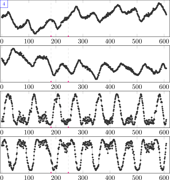
Figure 7: Honey bee movement switches between three states: left turn, right turn, and waggle. This series contains the $x$ position, $y$ position, and the sine and cosine of the head angle of a single bee. Data obtained from Oh et al. (2008).

[capbesideposition=left,top,capbesidewidth=5cm]figure[9cm]bitcoin

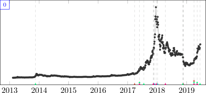
Figure 8: The price of Bitcoin in USD. Data obtained from Blockchain.com.

[capbesideposition=left,top,capbesidewidth=5cm]figure[9cm]brent_spot

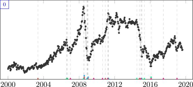
Figure 9: The price of Brent Crude oil in USD per barrel. Significant changes appear around 2008 and 2014. The data is sampled at every 10 original observations to reduce the length of the series. Obtained from the U.S. Energy Information Administration.

[capbesideposition=left,top,capbesidewidth=5cm]figure[9cm]businv

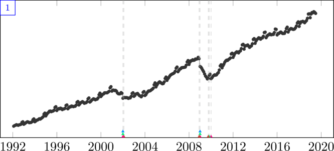
Figure 10: Monthly total business inventories (in USD), obtained from the U.S. Census Bureau. Effects of the financial crisis are visible. The non-seasonally-adjusted series is used to maintain the periodic component.

[capbesideposition=left,top,capbesidewidth=5cm]figure[9cm]centralia

Figure 11: The population of the mining town of Centralia, Pennsylvania, U.S., where a mine fire has been burning since 1962. Eminent domain was invoked in 1992, condemning all buildings in the town. Data obtained from Wikipedia.

[capbesideposition=left,top,capbesidewidth=5cm]figure[9cm]children_per_woman

Figure 12: The global average number of children born per woman. Data obtained from GapMinder.

[capbesideposition=left,top,capbesidewidth=5cm]figure[9cm]co2_canada

Figure 13: $\text{CO}_{2}$ emissions per person in Canada. Data obtained from GapMinder.

[capbesideposition=left,top,capbesidewidth=5cm]figure[9cm]construction

Figure 14: Total private construction spending in the U.S. Data obtained from the U.S. Census Bureau.

[capbesideposition=left,top,capbesidewidth=5cm]figure[9cm]debt_ireland

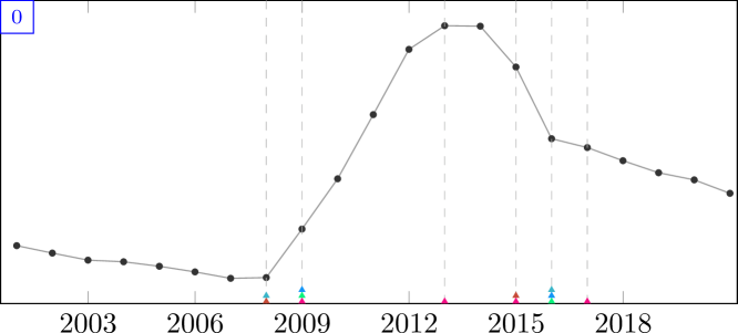
Figure 15: The government debt ratio of Ireland. Effects of the financial crisis of 2007–2008 are visible. Data obtained from EuroStat.

[capbesideposition=left,top,capbesidewidth=5cm]figure[9cm]gdp_argentina

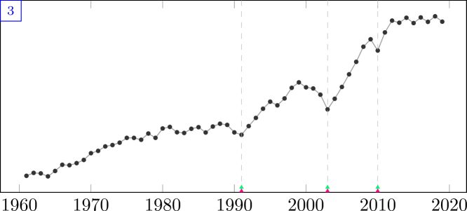
Figure 16: The GDP of Argentina in constant local currency. Data obtained from the World Bank.

[capbesideposition=left,top,capbesidewidth=5cm]figure[9cm]gdp_croatia

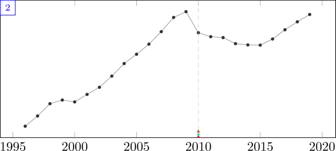
Figure 17: The GDP of Croatia in constant local currency. Data obtained from the World Bank.

[capbesideposition=left,top,capbesidewidth=5cm]figure[9cm]gdp_iran

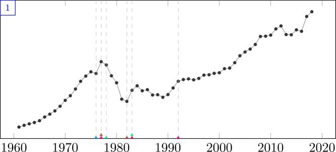
Figure 18: The GDP of Iran in constant local currency. Data obtained from the World Bank.

[capbesideposition=left,top,capbesidewidth=5cm]figure[9cm]gdp_japan

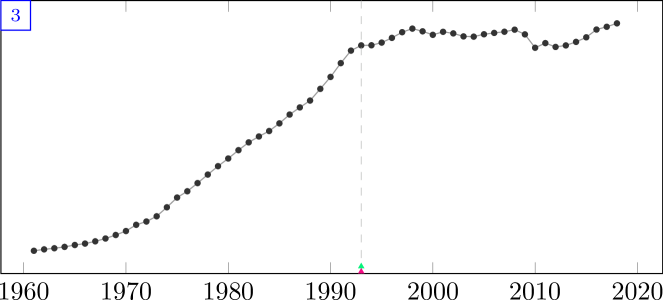
Figure 19: The GDP of Japan in constant local currency. Data obtained from the World Bank.

[capbesideposition=left,top,capbesidewidth=5cm]figure[9cm]global_co2

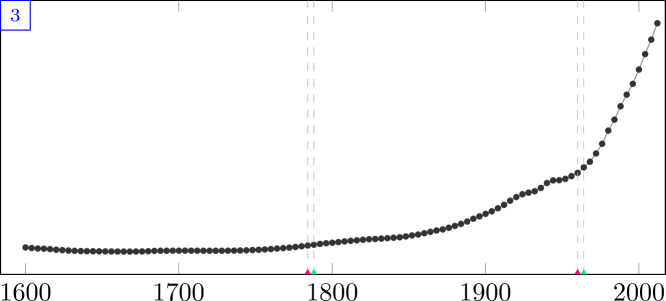
Figure 20: Monthly Global $\text{CO}_{2}$ levels. The series has been sampled every 48 months and cropped to recent history to reduce the length of the series. Data obtained from Meinshausen et al. (2017).

[capbesideposition=left,top,capbesidewidth=5cm]figure[9cm]homeruns

Figure 21: The number of home runs in the American League of baseball by year. Potentially significant events are the second world war and the Major League Baseball expansions. Data retrieved from the Baseball Databank.

[capbesideposition=left,top,capbesidewidth=5cm]figure[9cm]iceland_tourism

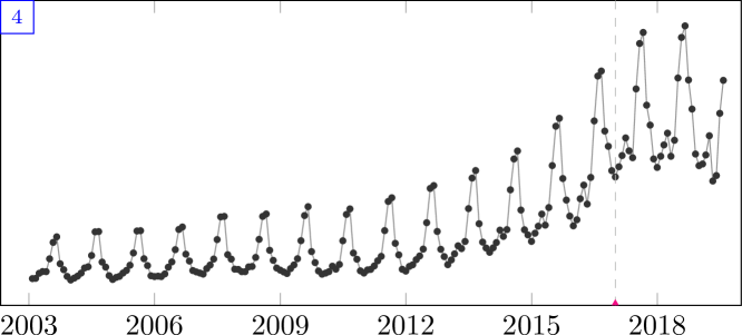
Figure 22: Monthly visitors to Iceland through Keflavik airport. Data obtained from the Icelandic Tourist Board.

[capbesideposition=left,top,capbesidewidth=5cm]figure[9cm]jfk_passengers

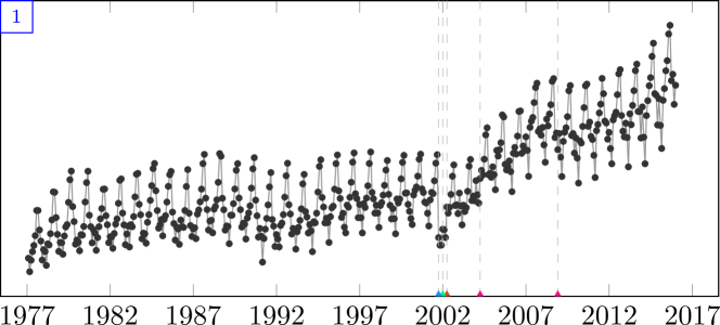
Figure 23: The number of passengers arriving and departing at John F. Kennedy airport in New York City. Data obtained from the Port Authority of New York and New Jersey.

[capbesideposition=left,top,capbesidewidth=5cm]figure[9cm]lga_passengers

[capbesideposition=left,top,capbesidewidth=5cm]figure[9cm]measles

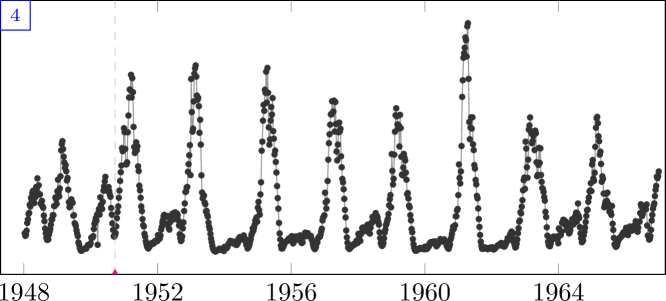
Figure 25: Number of measles cases in England and Wales over time. Data obtained from https://ms.mcmaster.ca/~bolker.

[capbesideposition=left,top,capbesidewidth=5cm]figure[9cm]nile

[capbesideposition=left,top,capbesidewidth=5cm]figure[9cm]occupancy

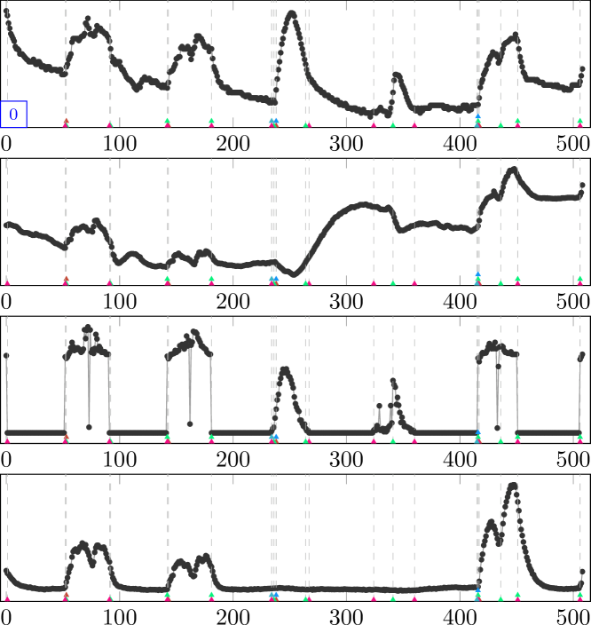
Figure 27: Room occupancy time series by Candanedo and Feldheim (2016) obtained from the UCI repository (Bache and Lichman, 2013). The four dimensions correspond to measurements of temperature, relative humidity, light, and $\text{CO}_{2}$. The original data has been sampled at every 16 observations to reduce the length of the series.

[capbesideposition=left,top,capbesidewidth=5cm]figure[9cm]ozone

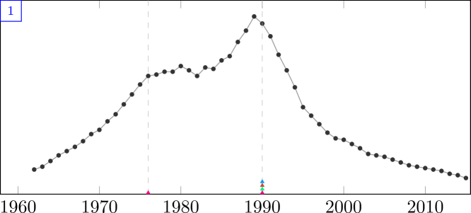
Figure 28: Levels of ozone-depleting substances in the atmosphere. The Montreal Protocol came into force in September 1989. Data from www.ourworldindata.org and originally due to Hegglin et al. (2015).

[capbesideposition=left,top,capbesidewidth=5cm]figure[9cm]rail_lines

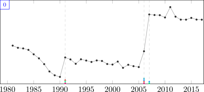
Figure 29: Total kilometers of rail lines in the world. Data obtained from the World Bank.

[capbesideposition=left,top,capbesidewidth=5cm]figure[9cm]ratner_stock

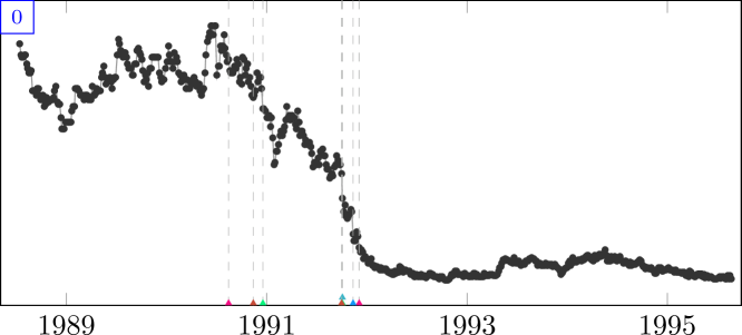
Figure 30: Stock price of the Ratner Group for a period in the early 1990s. Data obtained from Yahoo Finance and sampled every 3 observations to reduce the length of the series.

[capbesideposition=left,top,capbesidewidth=5cm]figure[9cm]robocalls

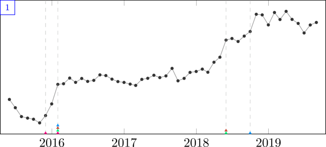
Figure 31: The number of automated phone calls in the U.S., which have been subject to varying degrees of regulation. Obtained from www.robocallindex.com.

[capbesideposition=left,top,capbesidewidth=5cm]figure[9cm]run_log

Figure 32: The pace and total distance traveled by a runner following an interval training program (alternating between running and walking). Data provided by the author.

[capbesideposition=left,top,capbesidewidth=5cm]figure[9cm]scanline_126007

Figure 33: A horizontal scan line of image no. 126007 from the Berkeley Segmentation Data Set (Martin et al., 2001).

[capbesideposition=left,top,capbesidewidth=5cm]figure[9cm]scanline_42049

Figure 34: A horizontal scan line of image no. 42049 from the Berkeley Segmentation Data Set (Martin et al., 2001).

[capbesideposition=left,top,capbesidewidth=5cm]figure[9cm]seatbelts

Figure 35: Number of drivers killed or seriously injured in the U.K. around the period of the introduction of seatbelts. Seatbelts were compulsory in new cars starting in 1972 and were mandatory to be worn from 1983 onwards. Obtained from the datasets package in R.

[capbesideposition=left,top,capbesidewidth=5cm]figure[9cm]shanghai_license

Figure 36: The number of applicants for a license plate in Shanghai. Data obtained from Kaggle.

[capbesideposition=left,top,capbesidewidth=5cm]figure[9cm]uk_coal_employ

[capbesideposition=left,top,capbesidewidth=5cm]figure[9cm]unemployment_nl

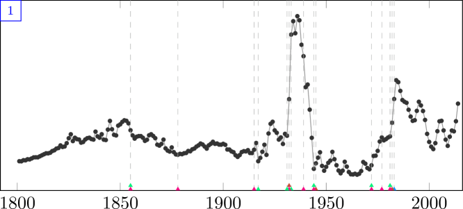
Figure 38: Unemployment rates in The Netherlands. Data obtained from Statistics Netherlands.

[capbesideposition=left,top,capbesidewidth=5cm]figure[9cm]usd_isk

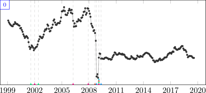
Figure 39: Exchange rate between the US Dollar and the Icelandic Króna in the years around the financial crisis. Data obtained from EuroStat.

[capbesideposition=left,top,capbesidewidth=5cm]figure[9cm]us_population

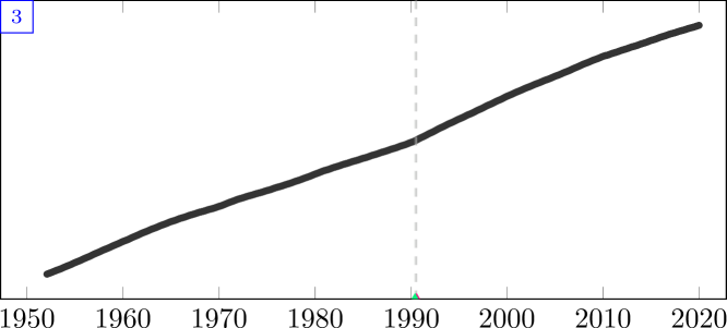
Figure 40: Population of the U.S. over time. Data obtained from the U.S. Census Bureau.

[capbesideposition=left,top,capbesidewidth=5cm]figure[9cm]well_log

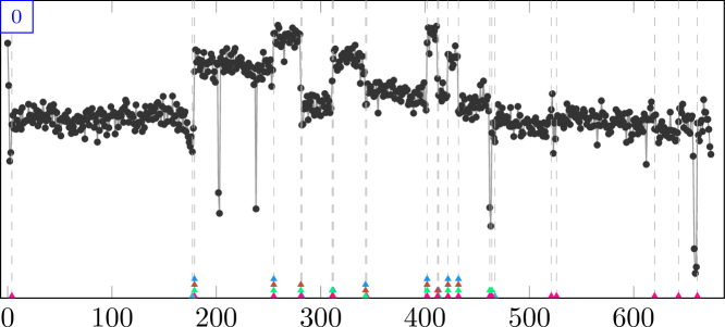
Figure 41: Well-log data from Ó Ruanaidh and Fitzgerald (1996). The series has been sampled every 6 iterations to reduce the length of the series.

D.2 Quality Control

This section lists the quality control data sets with known change points.

[capbesideposition=left,top,capbesidewidth=5cm]figure[9cm]quality_control_1

[capbesideposition=left,top,capbesidewidth=5cm]figure[9cm]quality_control_2

[capbesideposition=left,top,capbesidewidth=5cm]figure[9cm]quality_control_3

[capbesideposition=left,top,capbesidewidth=5cm]figure[9cm]quality_control_4

[capbesideposition=left,top,capbesidewidth=5cm]figure[9cm]quality_control_5

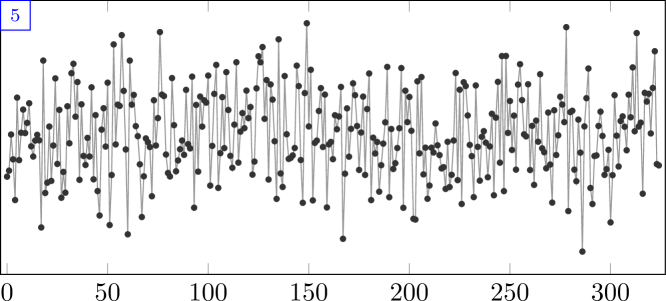
Figure 46: A series of $\mathcal{N}(0,1)$ noise without a change point.

D.3 Introductory Series

This section lists the synthetic time series shown to the annotators during the introduction. Since all annotators had to successfully complete the introduction before they could continue with real time series, the annotations are not shown for these series.

[capbesideposition=left,top,capbesidewidth=5cm]figure[9cm]demo_100

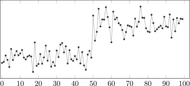
Figure 47: Series illustrating mean shift change point (index 50).

[capbesideposition=left,top,capbesidewidth=5cm]figure[9cm]demo_200

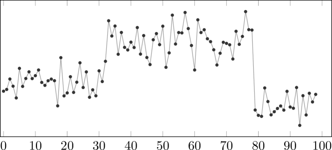
Figure 48: Series illustrating multiple change points (index 33 and 79).

[capbesideposition=left,top,capbesidewidth=5cm]figure[9cm]demo_300

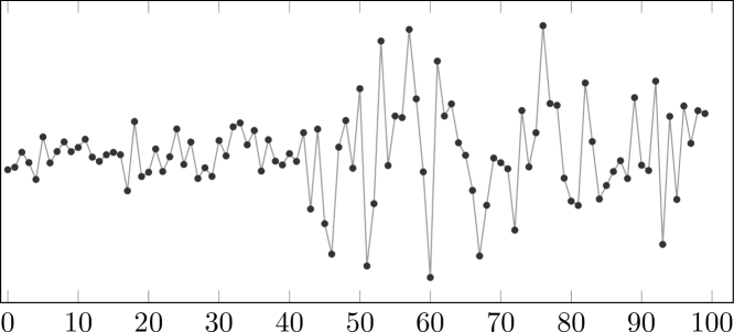
Figure 49: Series illustrating variance change (index 43).

[capbesideposition=left,top,capbesidewidth=5cm]figure[9cm]demo_400

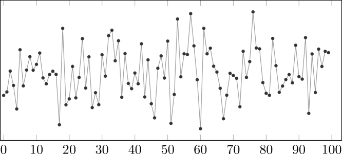
Figure 50: Series illustrating no change points.

[capbesideposition=left,top,capbesidewidth=5cm]figure[9cm]demo_500

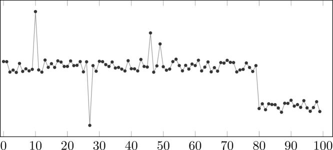
Figure 51: Series illustrating outliers and a mean shift change point (index 80).

[capbesideposition=left,top,capbesidewidth=5cm]figure[9cm]demo_600

Figure 52: Series illustrating a trend change (index 65).

[capbesideposition=left,top,capbesidewidth=5cm]figure[9cm]demo_650

Figure 53: Series illustrating a random walk (no change point).

[capbesideposition=left,top,capbesidewidth=5cm]figure[9cm]demo_700

Figure 54: Series illustrating a change in periodicity (index 57).

[capbesideposition=left,top,capbesidewidth=5cm]figure[9cm]demo_800

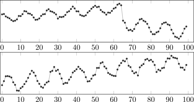
Figure 55: Series illustrating a multidimensional series with a change point in one dimension (index 65).

References

- Adams and MacKay (2007) Adams, R. P. and MacKay, D. J. C. Bayesian online changepoint detection. arXiv preprint arXiv:0710.3742, 2007.
- Aminikhanghahi and Cook (2017) Aminikhanghahi, S. and Cook, D. J. A survey of methods for time series change point detection. Knowledge and Information Systems, 51(2):339–367, 2017.
- Arabie and Boorman (1973) Arabie, P. and Boorman, S. A. Multidimensional scaling of measures of distance between partitions. Journal of Mathematical Psychology, 10(2):148–203, 1973.
- Arbelaez et al. (2010) Arbelaez, P., Maire, M., Fowlkes, C. C., and Malik, J. Contour detection and hierarchical image segmentation. IEEE Transactions on Pattern Analysis & Machine Intelligence, 33(5):898–916, 2010.
- Auger and Lawrence (1989) Auger, I. E. and Lawrence, C. E. Algorithms for the optimal identification of segment neighborhoods. Bulletin of Mathematical Biology, 51(1):39–54, 1989.
- Bache and Lichman (2013) Bache, K. and Lichman, M. UCI machine learning repository, 2013.
- Bai and Perron (2003) Bai, J. and Perron, P. Computation and analysis of multiple structural change models. Journal of Applied Econometrics, 18(1):1–22, 2003.
- Benavoli et al. (2016) Benavoli, A., Corani, G., and Mangili, F. Should we really use post-hoc tests based on mean-ranks? The Journal of Machine Learning Research, 17(1):152–161, 2016.
- Boracchi et al. (2018) Boracchi, G., Carrera, D., Cervellera, C., and Macciò, D. QuantTree: Histograms for change detection in multivariate data streams. In Proceedings of the 35th International Conference on Machine Learning, edited by Dy, J. and Krause, A., volume 80 of Proceedings of Machine Learning Research, pp. 639–648. PMLR, 2018.
- Candanedo and Feldheim (2016) Candanedo, L. M. and Feldheim, V. Accurate occupancy detection of an office room from light, temperature, humidity and measurements using statistical learning models. Energy and Buildings, 112:28–39, 2016.
- Chow (1960) Chow, G. C. Tests of equality between sets of coefficients in two linear regressions. Econometrica, 28:591–605, 1960.
- Demšar (2006) Demšar, J. Statistical comparisons of classifiers over multiple data sets. Journal of Machine Learning Research, 7:1–30, 2006.
- Durbin and Koopman (2012) Durbin, J. and Koopman, S. J. Time series analysis by state space methods. Oxford University Press, 2012.
- Everingham et al. (2010) Everingham, M., Van Gool, L., Williams, C. K. I., Winn, J., and Zisserman, A. The PASCAL Visual Object Classes (VOC) Challenge. International Journal of Computer Vision, 88(2):303–338, 2010.
- Fearnhead and Liu (2007) Fearnhead, P. and Liu, Z. On-line inference for multiple changepoint problems. Journal of the Royal Statistical Society: Series B (Statistical Methodology), 69(4):589–605, 2007.
- Fearnhead and Rigaill (2019) Fearnhead, P. and Rigaill, G. Changepoint detection in the presence of outliers. Journal of the American Statistical Association, 114(525):169–183, 2019.
- Friedman (1937) Friedman, M. The use of ranks to avoid the assumption of normality implicit in the analysis of variance. Journal of the American Statistical Association, 32(200):675–701, 1937.
- Friedman (1940) Friedman, M. A comparison of alternative tests of significance for the problem of rankings. The Annals of Mathematical Statistics, 11(1):86–92, 1940.
- Fryzlewicz (2014) Fryzlewicz, P. Wild binary segmentation for multiple change-point detection. The Annals of Statistics, 42(6):2243–2281, 2014.
- Garnett et al. (2009) Garnett, R., Osborne, M. A., and Roberts, S. J. Sequential Bayesian prediction in the presence of changepoints. In Proceedings of the 26th International Conference on Machine Learning, edited by Bottou, L. and Littman, M., pp. 345–352. Omnipress, 2009.
- Harchaoui et al. (2009) Harchaoui, Z., Moulines, E., and Bach, F. R. Kernel change-point analysis. In Advances in Neural Information Processing Systems, edited by Bengio, Y., Schuurmans, D., Lafferty, J. D., Williams, C. K. I., and Culotta, A., volume 22, pp. 609–616. Curran Associates, Inc., 2009.
- Hausdorff (1927) Hausdorff, F. Mengenlehre. Walter de Gruyter Berlin, 1927.
- Haynes et al. (2017) Haynes, K., Fearnhead, P., and Eckley, I. A. A computationally efficient nonparametric approach for changepoint detection. Statistics and Computing, 27(5):1293–1305, 2017.
- Hegglin et al. (2015) Hegglin, M. I., Fahey, D. W., McFarland, M., Montzka, S. A., and Nash, E. R. Twenty Questions and Answers About the Ozone Layer: 2014 Update, Scientific Assessment of Ozone Depletion: 2014. World Meteorological Organization, 2015.
- Hinkley (1970) Hinkley, D. V. Inference about the change-point in a sequence of random variables. Biometrika, 57(1):1–17, 1970.
- Hocking et al. (2014) Hocking, T. D., Boeva, V., Rigaill, G., Schleiermacher, G., Janoueix-Lerosey, I., Delattre, O., Richer, W., Bourdeaut, F., Suguro, M., Seto, M., Bach, F. R., and Vert, J.-P. SegAnnDB: interactive web-based genomic segmentation. Bioinformatics, 30(11):1539–1546, 2014.
- Hocking et al. (2013a) Hocking, T. D., Rigaill, G., Vert, J.-P., and Bach, F. R. Learning sparse penalties for change-point detection using max margin interval regression. In Proceedings of the 30th International Conference on Machine Learning, edited by Dasgupta, S. and McAllester, D., volume 28 of Proceedings of Machine Learning Research, pp. 172–180. PMLR, 2013a.
- Hocking et al. (2013b) Hocking, T. D., Schleiermacher, G., Janoueix-Lerosey, I., Boeva, V., Cappo, J., Delattre, O., Bach, F. R., and Vert, J.-P. Learning smoothing models of copy number profiles using breakpoint annotations. BMC Bioinformatics, 14(1):164, 2013b.
- Holm (1979) Holm, S. A simple sequentially rejective multiple test procedure. Scandinavian Journal of Statistics, 6(2):65–70, 1979.
- Hubert and Arabie (1985) Hubert, L. and Arabie, P. Comparing partitions. Journal of Classification, 2(1):193–218, 1985.
- Jackson et al. (2005) Jackson, B., Scargle, J. D., Barnes, D., Arabhi, S., Alt, A., Gioumousis, P., Gwin, E., Sangtrakulcharoen, P., Tan, L., and Tsai, T. T. An algorithm for optimal partitioning of data on an interval. IEEE Signal Processing Letters, 12(2):105–108, 2005.
- James and Matteson (2013) James, N. A. and Matteson, D. S. ecp: An R package for nonparametric multiple change point analysis of multivariate data. arXiv preprint arXiv:1309.3295, 2013.
- Killick and Eckley (2014) Killick, R. and Eckley, I. A. changepoint: An R package for changepoint analysis. Journal of Statistical Software, 58(3):1–19, 2014.
- Killick et al. (2012) Killick, R., Fearnhead, P., and Eckley, I. A. Optimal detection of changepoints with a linear computational cost. Journal of the American Statistical Association, 107(500):1590–1598, 2012.
- Knoblauch and Damoulas (2018) Knoblauch, J. and Damoulas, T. Spatio-temporal Bayesian on-line changepoint detection with model selection. In Proceedings of the 35th International Conference on Machine Learning, edited by Dy, J. and Krause, A., volume 80 of Proceedings of Machine Learning Research, pp. 2718–2727. PMLR, 2018.
- Knoblauch et al. (2018) Knoblauch, J., Jewson, J. E., and Damoulas, T. Doubly robust Bayesian inference for non-stationary streaming data with -divergences. In Advances in Neural Information Processing Systems, edited by Bengio, S., Wallach, H., Larochelle, H., Grauman, K., Cesa-Bianchi, N., and Garnett, R., volume 31, pp. 64–75. Curran Associates, Inc., 2018.
- Kurt et al. (2018) Kurt, B., Yıldız, Ç., Ceritli, T. Y., Sankur, B., and Cemgil, A. T. A Bayesian change point model for detecting SIP-based DDoS attacks. Digital Signal Processing, 77:48–62, 2018.
- Lavielle and Teyssiere (2007) Lavielle, M. and Teyssiere, G. Adaptive detection of multiple change-points in asset price volatility. In Long Memory in Economics, pp. 129–156. Springer, 2007.
- Lorden (1971) Lorden, G. Procedures for reacting to a change in distribution. The Annals of Mathematical Statistics, 42(6):1897–1908, 1971.
- Maidstone et al. (2017) Maidstone, R., Hocking, T. D., Rigaill, G., and Fearnhead, P. On optimal multiple changepoint algorithms for large data. Statistics and Computing, 27(2):519–533, 2017.
- Martin et al. (2004) Martin, D. R., Fowlkes, C. C., and Malik, J. Learning to detect natural image boundaries using local brightness, color, and texture cues. IEEE Transactions on Pattern Analysis & Machine Intelligence, 26(5):530–549, 2004.
- Martin et al. (2001) Martin, D. R., Fowlkes, C. C., Tal, D., and Malik, J. A database of human segmented natural images and its application to evaluating segmentation algorithms and measuring ecological statistics. In Proceedings of the 8th IEEE International Conference on Computer Vision, volume 2, pp. 416–423. IEEE, 2001.
- Matteson and James (2014) Matteson, D. S. and James, N. A. A nonparametric approach for multiple change point analysis of multivariate data. Journal of the American Statistical Association, 109(505):334–345, 2014.
- Meinshausen et al. (2017) Meinshausen, M., Vogel, E., Nauels, A., Lorbacher, K., Meinshausen, N., Etheridge, D. M., Fraser, P. J., Montzka, S. A., Rayner, P. J., Trudinger, C. M., Krummel, P. B., Beyerle, U., Canadell, J. G., Daniel, J. S., Enting, I. G., Law, R. M., Lunder, C. R., O’Doherty, S., Prinn, R. G., Reimann, S., Rubino, M., Velders, G. J. M., Vollmer, M. K., Wang, R. H. J., and Weiss, R. Historical greenhouse gas concentrations for climate modelling (CMIP6). Geoscientific Model Development, 10:2057–2116, 2017.
- Nemenyi (1963) Nemenyi, P. B. Distribution-free multiple comparisons. Ph.D. thesis, Princeton University, 1963.
- Oh et al. (2008) Oh, S. M., Rehg, J. M., Balch, T., and Dellaert, F. Learning and inferring motion patterns using parametric segmental switching linear dynamic systems. International Journal of Computer Vision, 77(1-3):103–124, 2008.
- Ó Ruanaidh and Fitzgerald (1996) Ó Ruanaidh, J. J. K. and Fitzgerald, W. J. Numerical Bayesian Methods Applied to Signal Processing. Springer, 1996.
- Page (1954) Page, E. S. Continuous inspection schemes. Biometrika, 41(1/2):100–115, 1954.
- Pagotto (2019) Pagotto, A. ocp: Bayesian Online Change Point Detection, 2019. R package version 0.1.1.
- Rigaill (2015) Rigaill, G. A pruned dynamic programming algorithm to recover the best segmentations with 1 to change-points. Journal de la Société Française de Statistique, 156(4):180–205, 2015.
- Saatçi et al. (2010) Saatçi, Y., Turner, R. D., and Rasmussen, C. E. Gaussian process change point models. In Proceedings of the 27th International Conference on Machine Learning, edited by Fürnkranz, J. and Joachims, T., pp. 927–934. Omnipress, 2010.
- Scott and Knott (1974) Scott, A. J. and Knott, M. A cluster analysis method for grouping means in the analysis of variance. Biometrics, 30(3):507–512, 1974.
- Taylor and Letham (2018) Taylor, S. J. and Letham, B. Forecasting at scale. The American Statistician, 72(1):37–45, 2018.
- Truong et al. (2017) Truong, C., Oudre, L., and Vayatis, N. Penalty learning for changepoint detection. In 25th European Signal Processing Conference, pp. 1569–1573. IEEE, 2017.
- Truong et al. (2020) Truong, C., Oudre, L., and Vayatis, N. Selective review of offline change point detection methods. Signal Processing, 167, 2020.
- Turner et al. (2009) Turner, R. D., Saatçi, Y., and Rasmussen, C. E. Adaptive sequential Bayesian change point detection. In Temporal Segmentation Workshop at NIPS, edited by Harchaoui, Z., 2009.
- Van Rijsbergen (1979) Van Rijsbergen, C. J. Information Retrieval. Butterworths, 1979.
- Wilcoxon (1945) Wilcoxon, F. Individual comparisons by ranking methods. Biometrics Bulletin, 1:80–83, 1945.