Long-term Prediction of Vehicle Behavior using Short-term
Uncertainty-aware Trajectories and High-definition Maps

Abstract

Motion prediction of surrounding vehicles is one of the most important tasks handled by a self-driving vehicle, and represents a critical step in the autonomous system necessary to ensure safety for all the involved traffic actors. Recently a number of researchers from both academic and industrial communities have focused on this important problem, proposing ideas ranging from engineered, rule-based methods to learned approaches, shown to perform well at different prediction horizons. In particular, while for longer-term trajectories the engineered methods outperform the competing approaches, the learned methods have proven to be the best choice at short-term horizons. In this work we describe how to overcome the discrepancy between these two research directions, and propose a method that combines the disparate approaches under a single unifying framework. The resulting algorithm fuses learned, uncertainty-aware trajectories with lane-based paths in a principled manner, resulting in improved prediction accuracy at both shorter- and longer-term horizons. Experiments on real-world, large-scale data strongly suggest benefits of the proposed unified method, which outperformed the existing state-of-the-art. Moreover, following offline evaluation the proposed method was successfully tested onboard a self-driving vehicle.

I Introduction

While self-driving vehicles (SDVs) have only recently entered the spotlight, the technology has been under active development for a long time [1], spanning decades of innovations and breakthroughs. There are several avenues proposed to solve the autonomy puzzle, with proposed ideas ranging from end-to-end systems [2, 3] to complex engineered frameworks with multiple interconnected components. Such engineered systems commonly consist of several modules operating in a sequence [4, 5], ranging from perception that takes sensors as inputs and performs detection and tracking of the surrounding actors, over prediction tasked with modeling the uncertain future, to motion planning that computes the SDV’s path in this stochastic environment [6]. In this work we consider the prediction problem, focusing on taking the tracked objects and predicting how will they move in the near future. While all the modules operate together to ensure safe and efficient behavior of the autonomous vehicle, predicting future motion of traffic actors in SDV’s surroundings is one of the critical steps, necessary for safe route planning. This was clearly exemplified by the collision between MIT’s “Talos” and Cornell’s “Skyne” vehicles during the 2007 DARPA Urban Challenge [7], where the lack of reasoning about intentions of other actors in the scene led to one of the first ever recorded collisions between two SDVs.

Motion prediction is not an easy task even for humans, owing to the stochasticity and complexity of the environment. Due to the vehicle inertia simple physics-based methods are accurate for very short predictions, yet beyond roughly one second they break as traffic actors constantly monitor their surroundings and need to promptly modify their behavior in response. Improving over ballistic methods, learned approaches have been shown to achieve good results in the short-term [8], defined as up to 3 seconds for the purposes of this paper. At longer horizons more complex models are required, where map-based approaches have shown promise [9]. However, these approaches are not good at handling unusual cases, such as actors performing illegal maneuvers. We address this problem, and propose a system that seamlessly fuses learned- and long-term predictions, taking into account factors such as the surrounding actors and map constraints, as well as uncertainty of the actor motion. In this way the resulting approach takes the best of the both worlds, allowing good accuracy at short- and long-term while handling outliers well. The method was compared to the state-of-the-art on a large-scale, real-world data where it provided strong performance across a wide range of prediction horizons.

Main contributions of our work are summarized below:

• we propose a method to unify state-of-the-art short- and long-term trajectories using a principled framework;

• extensive evaluation on large-scale, real-world data set showed that the proposed approach performs well across wide range of prediction horizons;

• following offline experiments, the method was successfully tested onboard a self-driving vehicle.

II Related work

Recently many researchers from both industry and academia turned their attention to the problem of motion prediction in traffic. This has led to a number of relevant works being proposed in the literature [10], ranging from engineered approaches that rely on manually specified rules to learned approaches based on the state-of-the-art deep architectures. In this section we give an overview of the existing publications most relevant for our current work.

A number of deployed methods in practice are based on engineered approaches, without the use of learned algorithms. In most systems the surrounding vehicles and other actors are tracked using Kalman filter (KF) [11], with tracked state including position, velocity, acceleration, heading, and other relevant quantities, to be used as an input to the downstream prediction methods. In [9] a deployed system by Mercedes-Benz is described, where the authors use the current actor state and the map information to associate an actor to nearby lanes, and future trajectories are inferred by propagating the current state along the associated lanes. In Honda’s system [12], the authors propagate KF state in time to predict short-term trajectories. Conversely, for longer-term predictions they use a similar lane-based idea as [9] by implicitly associating actors to lanes and computing time-to-collision to decide whether the SDV should stop or proceed in intersections. Unlike these approaches that do not apply learned methods, we propose to combine learned and engineered models to simultaneously improve both short- and long-term accuracy of predicted trajectories.

An interesting research direction for long-term motion prediction is inferring occupancy grids, as opposed to trajectories. In [13] the authors perform lane association similarly to [9], followed by discretization of a lane path into spatial cells and predicting likelihood that an actor will occupy a certain cell in the near future. Along similar lines, the authors of [14] applied grid-based prediction to pedestrian actors. While allowing for longer-term prediction, it is however not obvious how to extract actual trajectories which is a topic of our work. Another popular approach to long-term prediction is to compare a current motion to a set of historical actor behaviors and use the matched trajectories to infer the future. In [15] and [16] the authors use a longest common subsequence similarity measure to track the best historical hypothesis, while in [17] a dynamic-time warping is used to compute similarity. However, such approaches are not feasible in an online setting as they carry too large a cost when considering required memory and latency constraints.

As an alternative to explicitly inferring trajectories or occupancies, a common approach is predicting intents of surrounding actors, such as inferring lane-keeping or lane-changing behavior. The high-level intents can then be used to compute safe and efficient route of the autonomous vehicle. In [18], the authors propose energy-based approach to predict such intents. The authors of [19] train a multi-class classifier to predict lane changes, while [20] employ a Markovian process with extended KF. In [21] the authors take a step further and in addition to intents also predict short-term trajectories that obey the intended intent using Gaussian mixture model. In [22] they extended the work to use deep recurrent networks, showing improved performance. Similar deep learning-based approach was taken in a recent work [23]. Unlike these efforts, in the current work we assume that the intention (or goal) of a vehicle actor is already known, and we focus on prediction of realistic and accurate long-term trajectory that realizes such intent.

The success of deep learning has led to its wider adoption within the self-driving community as well. The authors of [8] proposed to rasterize the surrounding map and actors into a bird’s-eye view (BEV) raster, and use the resulting image as an input to deep convolutional neural network (CNN). The idea was later extended to multimodal predictions [24], yet unlike this work that uses a mixture model, we handle the multimodality through developing trajectories for multiple associated lanes. In [25] the authors used similar BEV approach to predict motion and control the SDV itself, while in [26] the authors proposed to perform both detection and prediction simultaneously. In a followup work [27], the authors proposed to predict intents as well (e.g., inferring if the actor will stay in the lane or come to a stop). However, an important downside of the existing work is that most of the published work is focused on short-term predictions, without considering longer horizons. This is due to the fact that the complexity of longer-term predictions grows exponentially as we increase the prediction horizon, requiring more data and more complex models to reach good performance [8]. In our work we propose to address this problem by combining short-term trajectories coming from learned models with long-term actor goals derived from associated lanes, referred to as Uncertainty-aware Stitching (US), resulting in improved performance at a wide range of prediction horizons.

III Proposed framework

We assume an output trajectory $\mathcal{T}=\{{\boldsymbol{\mu}}_{t},{\boldsymbol{\Sigma}}_{t}\}_{t=1}^{H}$ from a learned vehicle trajectory predictor is given, where each trajectory waypoint ${\bf w}_{t}$ is represented by a $2$-D Gaussian defined by mean ${\boldsymbol{\mu}}_{t}$ and covariance matrix ${\boldsymbol{\Sigma}}_{t}$, and given every $\Delta_{t}$ seconds for a total of $H$ time steps. Further, let $\mathcal{G}$ denote an intended goal path for a vehicle actor, represented as a polyline and obtained through associating the actor to nearby mapped lanes [9]. Then, the task is to determine a spatial path $\mathcal{S}$ of length $N$ ($N\geq H$) that captures both the short-term behavior from $\mathcal{T}$ and the long-term motion exhibited by an actor following $\mathcal{G}$, illustrated in Figure 1.

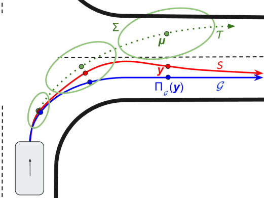
Figure 1: The proposed US method; green trajectory represents a short-term learned trajectory and associated uncertainties, blue is the goal path, and red is the solution path

We determine $\mathcal{S}$ in two steps. In section III-A we define an optimization problem for the first step, where we drop the dependence on $t$ for notational brevity. The optimization is done independently per trajectory waypoint to maximize the log-likelihood of a solution waypoint with respect to $\mathcal{T}$, regularized by a deviation cost to $\mathcal{G}$ (Sections III-A and III-B). This yields an initial part of the solution path that we refer to as a path prefix. Then, in the second step we extend the path beyond $H$ waypoints by smoothly interpolating the last prefix waypoint to the rest of $\mathcal{G}$ (Section III-C).

III-A Optimization for the path prefix

Conditioned on a goal $\mathcal{G}$ and waypoint parameters ${\boldsymbol{\mu}}$ and ${\boldsymbol{\Sigma}}$ of a trajectory $\mathcal{T}$, we would like to find the most likely position ${\bf y}$ of the resulting path prefix waypoint. To that end, we propose to solve the following optimization problem,

$$\operatorname*{arg\,max}_{\bf y}~{}\log\mathbb{P}({\bf y}\mid{\boldsymbol{\mu}},{\boldsymbol{\Sigma}})-\frac{\lambda}{2}\|{\bf y}-\Pi_{\mathcal{G}}({\bf y})\|^{2},$$ (1)

where $\Pi_{\mathcal{G}}({\bf y})$ denotes the projection of ${\bf y}$ onto the goal path $\mathcal{G}$, and $\lambda\geq 0$ is a parameter that controls the cost of goal deviation. As can be seen, we encourage ${\bf y}$ to remain in a high-support region of the predictive density, but penalize it if it deviates too much from the goal. As we assumed Gaussian distribution over trajectory waypoints, we can rewrite (1) as

$$\operatorname*{arg\,min}_{\bf y}~{}\|{\bf y}-{\boldsymbol{\mu}}\|_{{\boldsymbol{\Sigma}}^{-1}}^{2}+\lambda\min_{{\bf g}\in\mathcal{G}}\|{\bf y}-{\bf g}\|^{2},$$ (2)

where $\|{\bf v}\|_{{\bf Q}}=\sqrt{{\bf v}^{\top}{\bf Q}{\bf v}}$. An alternating minimization procedure can be used to approximately solve the problem. In particular, let $\mathcal{L}({\bf y},{\bf g})=\|{\bf y}-{\boldsymbol{\mu}}\|_{{\boldsymbol{\Sigma}}^{-1}}^{2}+\lambda\|{\bf y}-{\bf g}\|^{2}$. Then, for a given number of steps $M$, we find optimal ${\bf y}$ as follows,

• Initialize ${\bf y}^{0}={\boldsymbol{\mu}}$;

• For $m=1,\ldots,M$:

  • ${\bf g}^{m}=\arg\min_{{\bf g}\in\mathcal{G}}\|{\bf g}-{\bf y}^{m-1}\|^{2}$;

  • ${\bf y}^{m}=\arg\min_{{\bf y}}L({\bf y},{\bf g}^{m})$.

The above alternating minimizing procedure causes the objective function value $\mathcal{L}({\bf y},{\bf g})$ to decrease or remain the same in each iteration. Updates of both ${\bf g}$ and ${\bf y}$ can be computed efficiently. The ${\bf g}$-update can be solved by a search along the goal path, which takes linear time in the number of segments in a polyline representation of the goal path. The ${\bf y}$-update is a quadratic program with a closed-form solution.

III-B Dynamics of the solution path $\mathcal{S}$

The dynamics of the solution path obtained through (2) can be controlled by the regularization coefficient $\lambda$, which we choose to vary as a function of time (i.e., using $\lambda_{t}$, where $t=1,\ldots,H$). When considering which schedule to use for $\lambda_{t}$, we take into account the following desired properties of the solution path prefix $\{{\bf y}_{t}\}_{t=1}^{H}$:

• The first part of prefix $\{{\bf y}_{t}\}_{t=1}^{T}$ interpolates between $\mathcal{T}$ and $\mathcal{G}$, up to the last time horizon $T$ ($T\leq H$) where trajectory waypoint ${\bf w}_{T}$ is considered to be close to $\mathcal{G}$;

• The remainder $\{{\bf y}_{t}\}_{t=T+1}^{H}$ converges to $\mathcal{G}$ as $H\to\infty$.

As seen in the first property, we require a goodness or compatibility criterion that determines a time step $T$ when the solution path will start breaking away from the short-term trajectory. This is a topic of the following section.

III-B1 Waypoint compatibility score

Let $S({\bf w}_{t},\mathcal{G})\in[0,1]$ denote a compatibility score of the waypoint ${\bf w}_{t}$ w.r.t. $\mathcal{G}$, determined using the actor position distribution $\mathcal{N}({\boldsymbol{\mu}}_{t},{\boldsymbol{\Sigma}}_{t})$, a $2$-D polygon representation of actor shape at time step $t$ (denoted by $\mathcal{P}_{t}$), and the goal $\mathcal{G}$. The waypoint ${\bf w}_{t}$ is considered close to $\mathcal{G}$ iff $S({\bf w}_{t},\mathcal{G})\geq\alpha$, where $\alpha\in(0,1)$ is a fixed compatibility threshold.

To compute the compatibility score, we make the following assumptions: (i) actors are rigid-body objects; and (ii) average radius of turning paths is greater than average vehicle wheelbase. Assumption (i) enables us to determine the position uncertainty of any point ${\bf p}$ on the actor’s body using the distribution ${\mathcal{X}}_{\theta}=\mathcal{N}({\bf p},{\boldsymbol{\Sigma}}_{t})$, where $\theta$ are the distribution parameters. Let $D_{{\mathcal{X}}_{\theta}}({\bf x})=\|{\bf x}-{\bf p}\|_{{\boldsymbol{\Sigma}}_{t}^{-1}}$ represent the Mahalanobis distance of some point ${\bf x}$ from ${\mathcal{X}}_{\theta}$, and $\Pi_{\mathcal{G}}^{D_{{\mathcal{X}}_{\theta}}}({\bf p})=\operatorname*{arg\,min}_{{\bf g}\in\mathcal{G}}D_{{\mathcal{X}}_{\theta}}({\bf g})$ denote a function that computes the closest point on ${\mathcal{G}}$ from ${\bf p}$ based on the Mahalanobis distance. With a slight abuse of notation, let $S({\mathcal{X}}_{\theta},\mathcal{G})$ denote compatibility of the specified normal distribution ${\mathcal{X}}_{\theta}$ with $\mathcal{G}$,

$$S({\mathcal{X}}_{\theta},\mathcal{G})=\mathbb{P}\Big{(}D_{{\mathcal{X}}_{\theta}}\big{(}{\bf x})\geq D_{{\mathcal{X}}_{\theta}}(\Pi_{\mathcal{G}}^{D_{{\mathcal{X}}_{\theta}}}({\bf p})\big{)}\Big{)}.$$ (3)

where ${\bf x}\sim{\mathcal{X}}_{\theta}$. As ${\mathcal{X}}_{\theta}$ is a $2$-D Gaussian, equation (3) is equivalent to $S({\mathcal{X}}_{\theta},\mathcal{G})=\exp\big{(}-D_{{\mathcal{X}}_{\theta}}(\Pi_{\mathcal{G}}^{D_{{\mathcal{X}}_{\theta}}}({\bf p}))^{2}/2\big{)}$. This value can also be viewed as a p-value for the null hypothesis that $\Pi_{\mathcal{G}}^{D_{{\mathcal{X}}_{\theta}}}({\bf p})$ is a sample drawn from ${\mathcal{X}}_{\theta}$.

We use $S({\mathcal{X}}_{\theta},\mathcal{G})$ to determine $S({\bf w}_{t},\mathcal{G})$. If $\mathcal{P}_{t}$ overlaps the goal path polyline, we set $S({\bf w}_{t},\mathcal{G})=1$. Otherwise, $S({\bf w}_{t},\mathcal{G})=\max_{{\bf p}\in\mathcal{P}_{t}}S({\mathcal{X}}_{\theta},\mathcal{G})$. Assumption (ii) enables us to determine $S({\bf w}_{t},\mathcal{G})$ efficiently by considering the actor polygon vertices alone, without the need to account for the vertices of goal polyline. Then, we define $T$ as the latest time horizon $t$ at which $S({\bf w}_{t},\mathcal{G})\geq\alpha$, as

$$T=\max\big{\{}t:S({\bf w}_{t},\mathcal{G})\geq\alpha,t\in\{1,\ldots,H\}\big{\}}.$$ (4)

III-B2 Convergence of solution path to $\mathcal{G}$

We let the solution path interpolate between $\mathcal{T}$ and $\mathcal{G}$ up to horizon $T$, by setting $\lambda_{t}=\lambda_{0}$ for $t=1,\ldots,T$. After time step $T$, as there are no longer any waypoints ${\bf w}_{t}$ that are close to $\mathcal{G}$, we make the solution path converge to the goal path. This is done in order to avoid attributing a large weight to learned models at longer time horizons, where they are known to exhibit high uncertainties and to produce suboptimal predictions.

Let $f(t)$ be a non-negative, monotonically decreasing function of time. For a fixed constant $c>0$, we choose the following schedule for waypoints of the solution path,

$$\|{\bf y}_{t}-\Pi_{\mathcal{G}}({\bf y}_{t})\|=cf(t),$$ (5)

for $t=T+1,\ldots,H$. Using eigenvalue decomposition for the precision matrix ${\boldsymbol{\Sigma}}_{t}^{-1}={\bf Q}{\boldsymbol{\Lambda}}{\bf Q}^{\top}$, the closed-form for the ${\bf y}$ update step in Section III-A, and the assumption that $\lambda_{t}\gg|{\boldsymbol{\Lambda}}|_{\infty}$, we solve (5) approximately to obtain

$$\lambda_{t}=\frac{\|{\boldsymbol{\Sigma}}_{t}^{-1}\big{(}{\boldsymbol{\mu}}_{t}-\Pi_{\mathcal{G}}({\boldsymbol{\mu}}_{t})\big{)}\|}{cf(t)}.$$ (6)

The assumption is reasonable because as the time horizon increases position uncertainties increase as well, causing the eigenvalues of the precision matrix to decrease. Note that we only determine and set $\lambda_{t}$ once, and it stays constant for the remainder of the alternating optimization procedure. Lastly, this gives the following schedule for $\lambda_{t}$ when solving (2),

$$\lambda_{t}=\begin{cases}\lambda_{0},&\text{if }t\leq T,\\ \lambda_{0}+\frac{\|{\boldsymbol{\Sigma}}_{t}^{-1}({\boldsymbol{\mu}}_{t}-\Pi_{\mathcal{G}}({\boldsymbol{\mu}}_{t}))\|}{cf(t)},&\text{otherwise},\end{cases}\vspace{-.01in}$$ (7)

where $\lambda_{0}$ in the second case is included for continuity. We found the approximation in (6) to be effective in practice, and we set $f(t)=\frac{1}{t-T}$ in our experiments.

III-C Extending solution path $\mathcal{S}$ beyond $\mathcal{T}$

Let $\mathcal{G}^{\prime}$ represent the portion of $\mathcal{G}$ that was not used to produce the first $H$ points of $\mathcal{S}$. To generate a solution path $\{{\bf y}_{t}\}_{t=H+1}^{N}$ beyond ${\bf y}_{H}$ which may not lie on $\mathcal{G}$, for $t>H$ we shrink the offset between ${\bf y}_{t}$ and $\Pi_{\mathcal{G}}({\bf y}_{t})$ linearly with a sampling distance $s$ over a fixed distance of $d$ along $\mathcal{G}^{\prime}$ (with $s\leq d$). Lastly, we produce a full solution path $\mathcal{S}$ by attaching the remaining goal path starting from ${\bf y}_{H+\lfloor d/s\rfloor}$.

IV Experiments

For the purposes of empirical evaluation we used 240 hours of data collected by manually driving in various traffic conditions (e.g., varying times of day, days of the week, in several US cities) with data rate of $10Hz$, resulting in $\Delta_{t}=0.1s$. We ran a state-of-the-art detector and Unscented KF tracker on this data to produce a set of tracked vehicle detections. We removed all non-moving actors from the data, and separated the remainder into train/test/validation subsets using 3/1/1 split, used to train learned models and set parameters of the proposed method. We considered error metrics for horizons of up to 6 seconds with $1s$ increments.

For lane association of vehicle actors we considered all lanes within $100m$ radius from the actor position, and used as $\mathcal{G}$ the one with the smallest average $\ell_{2}$ distance to the ground-truth trajectory when computing error metrics. To obtain a short-term uncertainty-aware trajectory any learned trajectory prediction model can be chosen, and we used a state-of-the-art multi-modal RasterNet [8, 24], which uses BEV raster images of actors’ surroundings as input. The model outputs $6s$-long trajectories with a temporal resolution of $\Delta_{t}=0.1s$ ($H=60$). As the method outputs multiple trajectories, we used the one that was closest to the goal path in terms of the dynamic-time warping distance.

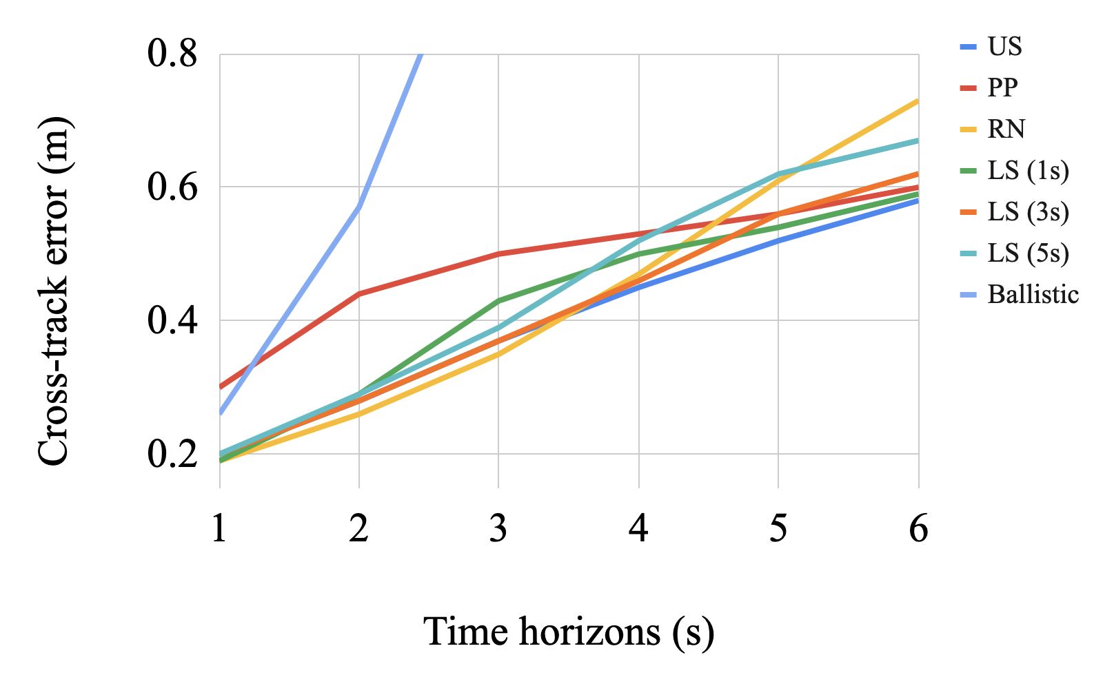
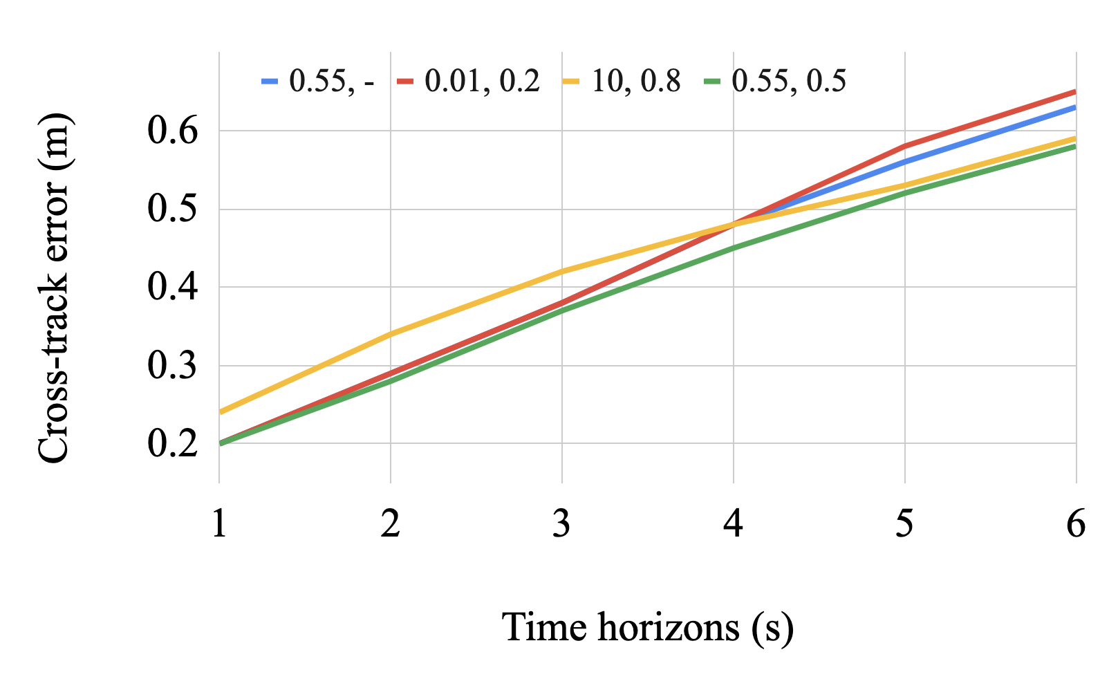
Figure 2: Comparison of cross-track error metrics (in meters): (a) against baselines, (b) across various $(\lambda_{0},\alpha)$ values

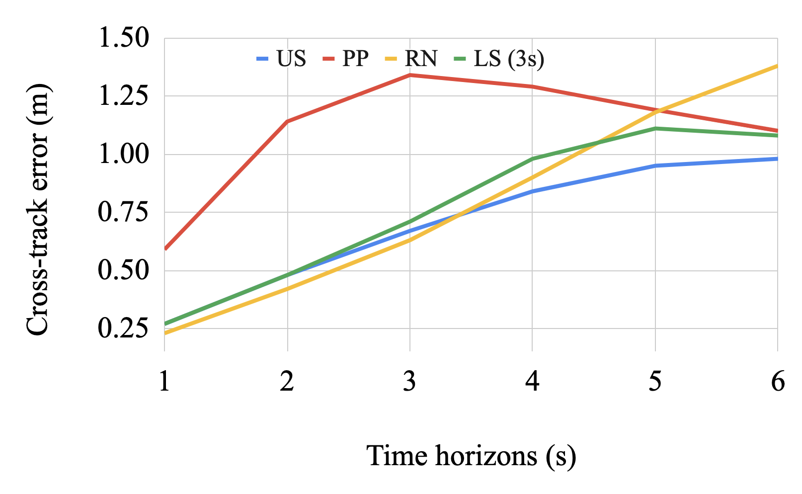
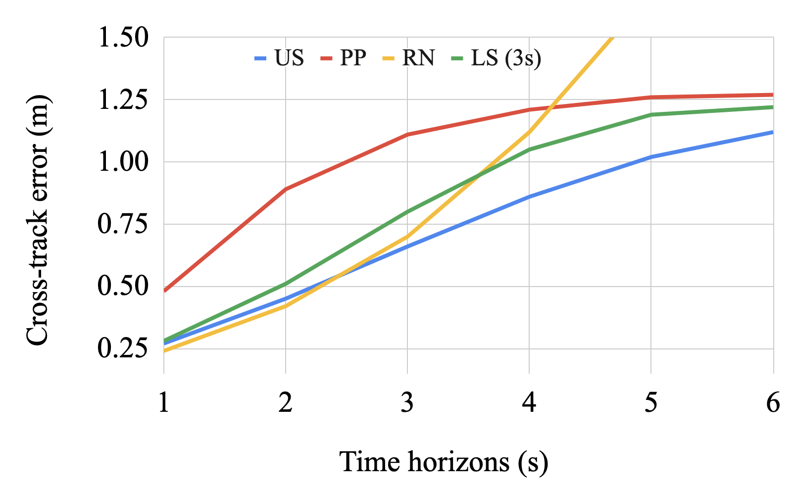
Figure 3: Comparison of cross-track error metrics (in meters) for: (a) left-turning; and (b) right-turning trajectories

Given an intended spatial path, we used the pure pursuit (PP) algorithm [28] to track the path and produce a spatio-temporal trajectory used for computing error metrics. In particular, we run PP iteratively to predict the actor’s next state, given the current one. We initialized the PP controller with the actor’s state at $t=0$ (including location, velocity, and acceleration), used a lookahead distance of $5m$, and made all actors move with a predefined speed profile. Here we used a simple scheme where the actor’s initial acceleration is maintained for $2s$, then decayed to zero with a jerk of $1m/s^{3}$, with the speed clamped between $0m/s$ and $15m/s$. We also imposed a turn radius constraint of $5m$ for regular-sized vehicles and $10m$ for larger vehicles, and executed two PP tracking steps within $0.1s$ to produce the next state.

As the proposed approach does not produce or modify the temporal signature of a trajectory (i.e., longitudinal motion of an actor), we focused solely on cross-track errors pertaining to spatial offsets from time-aligned waypoints across our approach and other baselines. The cross-track error of the output trajectory at a particular time horizon $t$ is defined as the distance between the predicted waypoint at $t$ and its projection to the ground-truth track. If the projection lies at one of the endpoints of the ground-truth track, we extend the ground truth linearly to infinity based on the heading direction at the endpoint, and recompute the error. To ensure time alignment and to remove possible confounding factors arising from longitudinal motion of actors across the competing methods, we retimed all learned model and ground-truth trajectories in the same manner. More specifically, retiming modifies a trajectory by recomputing arrival times for each of the trajectory’s waypoints, based on the simple speed profile described earlier which the actor is forced to follow.

IV-A Baselines and setup

To evaluate the performance of the proposed approach we compared it to several baselines, comprising pure physics-based models, control-based tracking algorithms, learned, and hybrid models. For the physics-based model we used a ballistic model that simply rolls out the current actor state into the future. The control-based algorithm we consider is pure pursuit described above, having it track $\mathcal{G}$ that best matches the ground truth (denoted as PP). For learned baselines we used RasterNet (RN) [8, 24], also introduced previously. As the method outputs three modes, for metrics we considered the mode with the lowest error. We also considered several hybrid methods that are equivalent to US where we do not take into account waypoint uncertainties. In particular, we instead stitch the first $n$ seconds of the RN trajectory with a goal path by following the procedure described in Section III-C, where we manually set the breakaway time step as $T=\lfloor n/\Delta_{t}\rfloor$. We denote these linear decay-stitching baselines by LS($n$), where $n\in\{1s,3s,5s\}$.

For our uncertainty-aware stitching approach, we set $\lambda_{0}=0.55$, $M=10$, $\alpha=0.5$, $c=1$, $s=1m$, and $d=10m$. These parameters were determined through a grid search based on cross-track error metrics across various time horizons. Lastly, to reduce onboard latency we approximated $\Pi_{\mathcal{G}}^{D_{{\mathcal{X}}_{\theta}}}({\bf p})$ in (3) by $\Pi_{\mathcal{G}}({\bf p})$, found to work well in practice.

IV-B Quantitative results

IV-B1 Comparison to baselines

We report cross-track (CT) errors across multiple time horizons in Figure 2(a) and Figure 3, where we compared the proposed US method to a number of baselines. We separately provide results computed only on turning examples in Figure 3, as left and right turns comprise only about 6% and 5.3% of our data set, respectively, and the results on these important maneuvers are lost when considering only the aggregate metrics.

In Figure 2(a) we see that the physics-based ballistic method severely underperforms, as it does not consider map features. On the other hand, the PP method produces trajectories that tend to stay as close as possible to the underlying goal path while respecting vehicle turn radius constraints. This is a reasonable prediction as vehicles usually do stay in their lanes over longer time horizon, resulting in lower CT error for $5s$ and $6s$ horizons. However, if we take a look at the results computed only on left and right turns in Figure 3, we can see a higher CT error since real-world actors tend to cut corners in turns which PP does not capture.

We can further see that RN does not perform well at longer horizons, which was observed in other work as well [8]. However, at short-term horizons RN exhibits strong performance and outperforms all other approaches. Learned models perform well in this regime, as they demonstrate greater ability to fit higher-order dynamics not explicitly modeled by rule-based systems such as pure pursuit. The LS($n$) methods are a combination of RN in the short term and PP in the long term, which is reflected in the results shown in Figures 2(a) and 3. We see in Figure 2(a) that as the fixed stitching horizon $n$ increases the metrics at longer horizons also degrade, as a longer portion of the RN trajectory is kept. On the other hand, we see that explicitly accounting for uncertainty through the US method leads to improvements over all LS($n$) methods where uncertainty is not considered and the stitching horizon is fixed. The proposed method exhibits very competitive performance across all horizons compared to the baselines, as it successfully combines good characteristics of short- and long-term-focused approaches.

IV-B2 Effect of varying stitching parameters

In Figure 2(b) we provide an ablation study of the US method, exploring the effect of various choices of $(\lambda_{0},\alpha)$ parameters. Note that the best parameter setting of $(0.55,0.5)$ discussed previously is also given to facilitate comparison. Setting the parameters to $(10,0.8)$ causes $\mathcal{S}$ to be close to $\mathcal{G}$, as any lateral deviation from the goal path would be penalized heavily. Moreover, it will also cause $\mathcal{S}$ to break away from $\mathcal{T}$ early on because of the high $\alpha$, causing the method to essentially fall back to pure pursuit being run directly on $\mathcal{G}$. Similarly, parameters $(0.01,0.2)$ encourage $\mathcal{S}$ to be closer to the mean of the learned uncertainty distributions, producing similar trajectories as the RN method. Thus, the proposed method can be viewed as a generalization of short- and long-term methods, which can be retrieved by tweaking the US parameters. We also see that setting $\lambda_{0}$ to be constant for all horizons, shown as $(0.55,-)$, performs poorly at longer horizons. This is because using constant values for $\lambda_{t}$ does not encourage $\mathcal{S}$ to converge to $\mathcal{G}$ after $\mathcal{T}$ diverges from it, and further motivates the proposed introduction of the compatibility score.

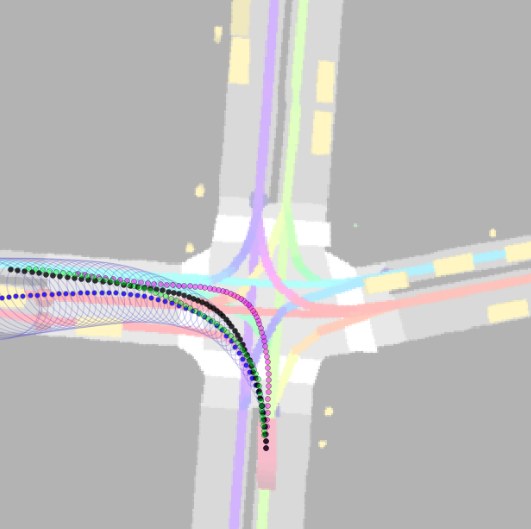
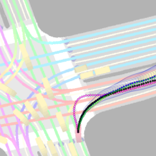
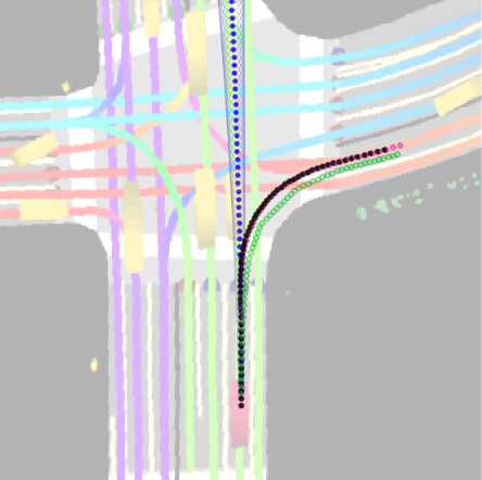
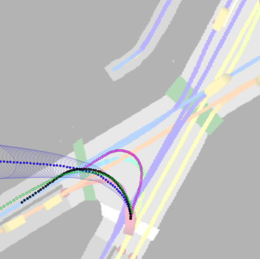
Figure 4: Comparison of baselines on commonly encountered scenarios; blue trajectory with uncertainties is the RN trajectory, purple trajectory is the PP trajectory, black trajectory is the US trajectory, while green trajectory is the ground-truth track

IV-C Qualitative results

In Figure 4 we give output trajectories of the competing methods on a set of commonly executed maneuvers: left turn, right turn, approaching intersection, and U-turn, respectively.

In both the left- and right-turn case the RN and the ground truth (GT) trajectories cut corners, while PP makes the actor follow the path exactly which does not capture reality well. In addition, for longer horizons RN trajectories veer off the actor’s lane into the neighboring lanes. As opposed to the baselines we see that the US method preserves both the short-term corner-cutting behavior and the long-term path-following behavior, thus closely following the GT trajectory.

In the third case RN incorrectly predicts that the actor will go straight, although $\mathcal{G}$ turns right. This causes US to break away early from RN and converge smoothly to $\mathcal{G}$, resulting in improved prediction. In the U-turn case, both RN and GT cut corners in the short term but the former quickly starts to veer off the road. As seen before, PP makes the actor follow $\mathcal{G}$ too closely, while the US trajectory combines the RN and PP outputs to obtain a very accurate future trajectory.

V Conclusion

In this study we addressed the critical problem of long-term traffic motion prediction of vehicle actors. While the existing work focuses either on short- or long-term performance such that accuracy on the other prediction horizon is sacrificed, we propose a method that obtains strong results for a wide range of prediction horizons. This is achieved by fusing short-term trajectories that are output by the state-of-the-art deep-learned models on one side, and long-term lane paths derived from a detailed high-definition map data on the other. Moreover, uncertainty of actor’s short-term motion is taken into account during the process, and is used to balance the impact of the two trajectory sources in a principled and consistent manner. We conducted a detailed evaluation of the proposed approach using a large-scale, real-world data collected by a fleet of self-driving vehicles, comparing the method to the existing state-of-the-art engineered and learned models. The results clearly indicate benefits of the proposed US algorithm, and following offline tests the method was successfully tested onboard an autonomous vehicle.

References

- [1] C. Urmson, “Progress in self-driving vehicles,” Frontiers of Engineering, pp. 5–9, 2015.
- [2] D. A. Pomerleau, Neural network perception for mobile robot guidance. Springer Science & Business Media, 2012, vol. 239.
- [3] M. Bojarski, D. Del Testa, D. Dworakowski, B. Firner, B. Flepp, P. Goyal, L. D. Jackel, M. Monfort, U. Muller, J. Zhang, et al., “End-to-end learning for self-driving cars,” arXiv preprint arXiv:1604.07316, 2016.
- [4] C. Urmson and W. Whittaker, “Self-driving cars and the urban challenge,” IEEE Intelligent Systems, vol. 23, no. 2, pp. 66–68, 2008.
- [5] C. Badue, R. Guidolini, R. V. Carneiro, P. Azevedo, V. B. Cardoso, A. Forechi, L. Jesus, R. Berriel, T. Paixão, F. Mutz, et al., “Self-driving cars: A survey,” arXiv preprint arXiv:1901.04407, 2019.
- [6] B. Paden, M. Čáp, S. Z. Yong, D. Yershov, and E. Frazzoli, “A survey of motion planning and control techniques for self-driving urban vehicles,” IEEE Transactions on intelligent vehicles, vol. 1, no. 1, pp. 33–55, 2016.
- [7] L. Fletcher, S. Teller, et al., The MIT – Cornell Collision and Why It Happened, 2009, p. 509–548.
- [8] N. Djuric, V. Radosavljevic, H. Cui, T. Nguyen, F.-C. Chou, T.-H. Lin, N. Singh, and J. Schneider, “Uncertainty-aware short-term motion prediction of traffic actors for autonomous driving,” IEEE Winter Conference on Applications of Computer Vision (WACV), 2020.
- [9] J. Ziegler, P. Bender, M. Schreiber, et al., “Making bertha drive - an autonomous journey on a historic route,” IEEE Intelligent Transportation Systems Magazine, vol. 6, pp. 8–20, 10 2015.
- [10] A. Rudenko, L. Palmieri, M. Herman, K. M. Kitani, D. M. Gavrila, and K. O. Arras, “Human motion trajectory prediction: A survey,” arXiv preprint arXiv:1905.06113, 2019.
- [11] R. E. Kalman, “A new approach to linear filtering and prediction problems,” Transactions of the ASME–Journal of Basic Engineering, vol. 82, no. Series D, pp. 35–45, 1960.
- [12] A. Cosgun, L. Ma, et al., “Towards full automated drive in urban environments: A demonstration in gomentum station, california,” in IEEE Intelligent Vehicles Symposium, 2017, pp. 1811–1818. [Online]. Available: https://doi.org/10.1109/IVS.2017.7995969
- [13] P. Kaniarasu, G. C. Haynes, and M. Marchetti-Bowick, “Goal-directed occupancy prediction for lane-following actors,” in IEEE International Conference on Robotics and Automation (ICRA), 2020.
- [14] A. Jain, S. Casas, R. Liao, Y. Xiong, S. Feng, S. Segal, and R. Urtasun, “Discrete residual flow for probabilistic pedestrian behavior prediction,” arXiv preprint arXiv:1910.08041, 2019.
- [15] C. Hermes, C. Wohler, K. Schenk, and F. Kummert, “Long-term vehicle motion prediction,” in 2009 IEEE intelligent vehicles symposium. IEEE, 2009, pp. 652–657.
- [16] C. Hermes, J. Einhaus, M. Hahn, C. Wöhler, and F. Kummert, “Vehicle tracking and motion prediction in complex urban scenarios,” in 2010 IEEE Intelligent Vehicles Symposium. IEEE, 2010, pp. 26–33.
- [17] K. Okamoto, K. Berntorp, and S. Di Cairano, “Similarity-based vehicle-motion prediction,” in 2017 American Control Conference (ACC). IEEE, 2017, pp. 303–308.
- [18] H. Woo, Y. Ji, H. Kono, Y. Tamura, Y. Kuroda, T. Sugano, Y. Yamamoto, A. Yamashita, and H. Asama, “Lane-change detection based on vehicle-trajectory prediction,” IEEE Robotics and Automation Letters, vol. 2, no. 2, pp. 1109–1116, 2017.
- [19] P. Kumar, M. Perrollaz, S. Lefevre, and C. Laugier, “Learning-based approach for online lane change intention prediction,” in 2013 IEEE Intelligent Vehicles Symposium (IV). IEEE, 2013, pp. 797–802.
- [20] R. Toledo-Moreo and M. A. Zamora-Izquierdo, “Imm-based lane-change prediction in highways with low-cost gps/ins,” IEEE Transactions on Intelligent Transportation Systems, vol. 10, no. 1, pp. 180–185, 2009.
- [21] N. Deo, A. Rangesh, and M. M. Trivedi, “How would surround vehicles move? a unified framework for maneuver classification and motion prediction,” IEEE Transactions on Intelligent Vehicles, vol. 3, no. 2, pp. 129–140, 2018.
- [22] N. Deo and M. M. Trivedi, “Multi-modal trajectory prediction of surrounding vehicles with maneuver based lstms,” in 2018 IEEE Intelligent Vehicles Symposium (IV). IEEE, 2018, pp. 1179–1184.
- [23] A. Zyner, S. Worrall, and E. Nebot, “Naturalistic driver intention and path prediction using recurrent neural networks,” IEEE Transactions on Intelligent Transportation Systems, 2019.
- [24] H. Cui, V. Radosavljevic, et al., “Multimodal trajectory predictions for autonomous driving using deep convolutional networks,” in IEEE International Conference on Robotics and Automation (ICRA), 2019.
- [25] M. Bansal, A. Krizhevsky, and A. Ogale, “Chauffeurnet: Learning to drive by imitating the best and synthesizing the worst,” arXiv preprint arXiv:1812.03079, 2018.
- [26] W. Luo, B. Yang, and R. Urtasun, “Fast and furious: Real time end-to-end 3d detection, tracking and motion forecasting with a single convolutional net,” in Proceedings of the IEEE CVPR, 2018, pp. 3569–3577.
- [27] S. Casas, W. Luo, and R. Urtasun, “Intentnet: Learning to predict intention from raw sensor data,” in Conference on Robot Learning, 2018, pp. 947–956.
- [28] R. C. Conlter, “Implementation of the pure pursuit path tracking algorithm,” 1992.