Joint Alignment From Pairwise Differences
with a Noisy Oracle

Abstract

In this work we consider the problem of recovering $n$ discrete random variables $x_{i}\in\{0,\ldots,k-1\},1\leq i\leq n$ (where $k$ is constant) with the smallest possible number of queries to a noisy oracle that returns for a given query pair $(x_{i},x_{j})$ a noisy measurement of their modulo $k$ pairwise difference, i.e., $y_{ij}=x_{i}-x_{j}\mod k$. This is a joint discrete alignment problem with important applications in computer vision [13, 30], graph mining [27], and spectroscopy imaging [29]. Our main result is a polynomial time algorithm that learns exactly with high probability the alignment (up to some unrecoverable offset) using $O(n^{1+o(1)})$ queries.

1 Introduction

Learning a joint alignment from pairwise differences is a problem with various important applications in computer vision [13, 30], graph mining such as predicting signed interactions in online social networks [27], databases such as entity resolution [17, 19, 20], and spectroscopy imaging [29]. Formally, there exists a set $V=[n]\mathrel{\stackrel{{\scriptstyle\makebox[0.0pt]{\mbox{\tiny def}}}}{{=}}}\{0,\ldots,n-1\}$ of $n$ discrete items labeled from $0$ to $n-1$, and an assignment $g:V\rightarrow[k]\mathrel{\stackrel{{\scriptstyle\makebox[0.0pt]{\mbox{\tiny def}}}}{{=}}}\{0,\ldots,k-1\}$ according to which each item is assigned one out of $k\geq 2$ possible values. The assignment function $g$ is unknown, but we obtain a set of corrupted samples of the pairwise differences $\{y_{i,j}\mathrel{\stackrel{{\scriptstyle\makebox[0.0pt]{\mbox{\tiny def}}}}{{=}}}g(i)-g(j)\mod k\}_{(i,j)\in\Omega}$, where $\Omega\subseteq[n]\times[n]$ is a symmetric index set, i.e., if $(i,j)\in\Omega$, implies $(j,i)\in\Omega$. To give an example, imagine a set of $n$ images of the same object, where each $g(i)$ is the orientation/angle of the camera when taking the $i$-th image. The goal is to recover $g$ based on these measurements, up to some global offset $c\in[k]$ that is unrecoverable. However, learning a joint alignment from such differences is a non-convex problem by nature, since the input space is discrete and already non-convex to begin with [5].

Model. We start with the following simplified model. Later we discuss how to apply our approach to a more general noise model. Let $0<q\leq\frac{1}{2}$, and suppose that there are $k$ groups, where $k$ is a positive constant, that we number $\{0,1,...,k-1\}$ and that we think of as being arranged modulo $k$. Let $g(u)$ refer to the group number associated with a vertex $u$. We are allowed to query a given pair of nodes only once. When we query a tuple of nodes $(x,y)$, we obtain an oracle answer $\tilde{f}(e)$ that is a random variable distributed according to the following equation:

$$\tilde{f}(e)=\left\{\begin{array}[]{lr}g(x)-g(y)\bmod k,&\text{with probability }1-q;\\ g(x)-g(y)+1\bmod k,&\text{with probability }q/2;\\ g(x)-g(y)-1\bmod k,&\text{with probability }q/2.\end{array}\right.$$ (1)

That is, we obtain the difference between the groups when no error occurs, and with probability $q$ we obtain an error that adds or subtracts one to this gap with equal probability. According to our model, once a tuple $(x,y)$ is queried, querying $(y,x)$ is not meaningful as it will provide no new information, i.e., it will be the additive inverse of the oracle answer for $(x,y)$ modulo $k$. In this work we ask the following question:

Our main contribution is the following result, stated as Theorem 1.

Theorem 1.

There exists a polynomial time algorithm that performs $O(n^{1+o(1)})$ queries, and recovers $g$ (up to some global offset) whp when $0<q\leq\frac{1}{2}$.

Our result extends our recent work on clustering with a faulty oracle [27], and relies on techniques developed therein. Clustering with a faulty oracle uses a querying model according to which the faulty oracle returns a noisy answer on whether two nodes belong to the same cluster or not [20, 27]. Learning joint alignments and clustering with a faulty oracle are equivalent when $k=2$, and become different for any $k\geq 3$. We analyze the fundamental case $k=2$ in Section 3, and then we show how our techniques extend to $k\geq 3$. For convenience, when $k=2$ we set the two cluster ids as $\{-1,+1\}$, rather than the two possible remainders of division by 2, i.e. $\{0,1\}$, as we do for the rest of the paper. It is worth outlining that using the algorithm from [27], cannot solve the joint alignment problem; indeed, even with no errors, a chain of responses on whether two nodes belong to the same cluster along a path would not generally allow us to determine whether the endpoints of a path were in the same group or not.

Our proposed algorithm can handle queries governed by more general error models, of the form:

$$\tilde{f}(e)=g(x)-g(y)+i\mod k\text{~{}~{}~{}with probability~{}}q_{i},0\leq i<k.$$

That is, the error does not depend on the group values $x$ and $y$, but is simply independent and identically distributed over the values $0$ to $k-1$. We outline how our algorithm adapts to this more general case.

Related work. Optimal results in terms of query complexity for an even more general version of this problem that allows for $k$ to be a non-constant function, were originally given by Chen and Candés [5]. In their work they study the general noise model. Again, each pair can be queried at most once, and the noisy measurement $\tilde{f}(x,y)$ is equal to

$$\tilde{f}(x,y)=\big{(}g(x)-g(y)+\eta_{xy}\big{)}\bmod k$$

where the additive noise values $\eta_{xy}$ are i.i.d. random variables supported on $\{0,1,\cdots,k-1\}$, with the following probability distribution that is slightly biased towards zero for some parameter $\delta>0$:

$${\bf{Pr}}\left[{\eta_{xy}=i}\right]=\left\{\begin{array}[]{lr}\frac{1}{k}+\delta,&\text{if }i=0;\\ \frac{1}{k}-\frac{\delta}{k-1},&\text{for each }i\neq 0.\\ \end{array}\right.$$

They design an algorithm that is non-adaptive, and the underlying queries form a random binomial graph [5], just our proposed method. Furthermore, Chen and Candès prove that for random binomial graph query graphs, the minimax probability of error tends to 1 if the number of queries is less than $\Omega\left(\frac{n\log n}{k\delta^{2}}\right)$ [5, Theorem 2,p. 7]. Their algorithm, based on the projected power method, has a required number of queries that matches the lower bound. Recently Larsen, Mitzenmacher, and Tsourakakis strenghtened the lower bound of Chen and Candés by proving that any non-adaptive algorithm requires $\Omega(\frac{n\log n}{k\delta^{2}})$ queries. Furthermore, they designed an (asymptotically) optimal, simple combinatorial algorithm both in terms of query and run time complexity [16]. The results in this work are suboptimal compared to [5, 16], but they use different algorithmic techniques that are possibly of independent interest.

2 Theoretical Preliminaries

We use the following probabilistic results for the proofs in Section 3.

Theorem 2 (Chernoff bound, Theorem 2.1 [14]).

Let $X\sim\text{Bin}\left(n,p\right)$, $\mu=np$, $a\geq 0$ and $\varphi(x)=(1+x)\ln(1+x)-x$ (for $x\geq-1$, or $\infty$ otherwise). Then the following inequalities hold:

$${\bf{Pr}}\left[{X\leq\mu-a}\right] \leq e^{-\mu\varphi\left(\frac{-a}{\mu}\right)}\leq e^{-\frac{a^{2}}{2\mu}},$$ (2)

$${\bf{Pr}}\left[{X\geq\mu+a}\right] \leq e^{-\mu\varphi\left(\frac{-a}{\mu}\right)}\leq e^{-\frac{a^{2}}{2(\mu+a/3)}}.$$ (3)

We define the notion of read-$k$ families, a useful concept when proving concentration results for weakly dependent variables.

Definition 1 (Read-$k$ families).

Let $X_{1},\dots,X_{m}$ be independent random variables. For $j\in[r]$, let $P_{j}\subseteq[m]$ and let $f_{j}$ be a Boolean function of $\{X_{i}\}_{i\in P_{j}}$. Assume that $|\{j|i\in P_{j}\}|\leq k$ for every $i\in[m]$. Then, the random variables $Y_{j}=f_{j}(\{X_{i}\}_{i\in P_{j}})$ are called a read-$k$ family.

The following result was proved by Gavinsky et al. for concentration of read-$k$ families. The intuition is that when $k$ is small, we can still obtain strong concentration results.

Theorem 3 (Concentration of Read-$k$ families [11]).

Let $Y_{1},\ldots,Y_{r}$ be a family of read-$k$ indicator variables with ${\bf{Pr}}\left[{Y_{i}=1}\right]=q$. Then for any $\epsilon>0$,

$${\bf{Pr}}\left[{\sum_{i=1}^{r}Y_{i}\geq(q+\epsilon)r}\right]\leq e^{-D_{\text{KL}}({q+\epsilon}||{q})\cdot r/k}$$ (4)

and

$${\bf{Pr}}\left[{\sum_{i=1}^{r}Y_{i}\leq(q-\epsilon)r}\right]\leq e^{-D_{\text{KL}}({q-\epsilon}||{q})\cdot r/k}.$$ (5)

Here, $D_{\text{KL}}$ is Kullback-Leibler divergence defined as

$$D_{\text{KL}}({q}||{p})=q\log{\left(\frac{q}{p}\right)}+(1-q)\log{\left(\frac{1-q}{1-p}\right)}.$$

The following corollary of Theorem 3 provides multiplicative Chernoff-type bounds for read-$k$ families. Notice that the parameter $k$ appears as an extra factor in denominator of the exponent, that is why when $k$ is relatively small we still obtain meaningful concentration results.

Theorem 4 (Concentration of Read-$k$ families [11]).

Let $Y_{1},\ldots,Y_{r}$ be a family of read-$k$ indicator variables with ${\bf{Pr}}\left[{Y_{i}=1}\right]=q$. Also, let $Y=\sum_{i=1}^{r}Y_{i}$. Then for any $\epsilon>0$,

$${\bf{Pr}}\left[{Y\geq(1+\epsilon){\mathbb{E}}\left[{Y}\right]}\right]\leq e^{-\frac{\epsilon^{2}{\mathbb{E}}\left[{Y}\right]}{2k(1+\epsilon/3)}}$$ (6)

$${\bf{Pr}}\left[{Y\leq(1-\epsilon){\mathbb{E}}\left[{Y}\right]}\right]\leq e^{-\frac{\epsilon^{2}{\mathbb{E}}\left[{Y}\right]}{2k}}.$$ (7)

3 Proposed Method

Proof strategy. Our proposed algorithm is heavily based on our work for the case $k=2$, a special case of the joint alignment problem of interest to the social networks’ community [27]. According to our, we may query any pair of nodes once, and we receive the correct answer on whether the two nodes are in the same cluster, or not, with probability $1-q=\frac{1+\delta}{2}$. Here, $0<\delta<1$ is the bias. In both cases $k=2$ and $k\geq 3$, the structure of the algorithmic analysis is identical. Let $L=\frac{\log{n}}{\log{\log{n}}}$. At a high level, our proof strategy is as follows:

1. We perform $n\Delta$ queries uniformly at random. We set $\Delta=O(\frac{\log{n}}{\delta^{L}})$.

2. We compute the probability that a path between $x$ and $y$ provides us with the correct information on $g(x)-g(y)$ or not.

3. We show that there exists a large number of almost edge-disjoint paths of length $L$ between any pair of vertices with probability at least $1-\frac{1}{n^{3}}$.

4. To learn the difference $g(x)-g(y)$ for any pair of nodes $\{x,y\}$, we take a majority vote ($k=2$), or a plurality vote ($k\geq 3$), among the paths we have created. A union bound in combination with (2) shows that whp we learn $g$ up to some uknown offset.

Algorithm 1 Learning Joint Alignment for $k=2$

  $L\leftarrow\frac{\log{n}}{\log{\log{n}}}$

  Perform $20n\log{n}\delta^{-L}$ queries uniformly at random.

  Let $G(V,E,\tilde{f})$ be the resulting graph, $\tilde{f}:E\rightarrow\{+1,-1\}$

  for each item pair $x,y$ do

     $\mathcal{P}_{x,y}=\{P_{1},\ldots,P_{N}\}\leftarrow$ Almost-Edge-Disjoint-Paths($x,y$)

     $Y_{i}\leftarrow\prod_{e\in P_{i}}\tilde{f}(e)$ for $i=1,\ldots,N$

     $Y_{xy}\leftarrow\sum_{P\in\mathcal{P}_{u,v}}Y_{P}$

     if $Y_{xy}\geq 0$ then

        predict $g(x)=g(y)$

     else

        predict $g(x)\neq g(y)$

     end if

  end for

Key differences with prior work [27]. While this work relies on [27], there are some key differences. Our main result in [27] is that when there exist two latent clusters ($k=2$), we can recover them whp using $O(n\log n/\delta^{4})$ queries, i.e., $\Delta=O(\log n/\delta^{4})$. In this work we need to set $\Delta=O(\log n\delta^{-L})$, i.e., we perform a larger number of queries. Here, $L=\frac{\log{n}}{\log{\log{n}}}$. An interesting open question is to reduce the number of queries when $k\geq 3$. Since the models are different, step 2 also differs. Furthermore, the algorithm proposed in [27], and the one we propose here are different; in [27] we use a recursive algorithm that we analyze using Fourier analysis to get a near-optimal result with respect to the number of queries. Here, we use concentration of multivariate polynomials [11], see also [3, 7, 15, 26], to analyze the plurality vote of the paths that we construct between a given pair of nodes. Steps 3, 4 are almost identical both in [27], and here. The key difference is that our algorithm requires an average degree $O\left(\frac{\log n}{\delta^{L}}\right)$ only for the first level of certain trees that we grow, for the rest of the levels a branching factor of order $O(\log n)$ suffices.

Algorithm 2 Almost-Edge-Disjoint-Paths($x,y$)

  Input: $G(V,E,\tilde{f})$, $x,y\in V(G)$

  Output: Set of paths between $x,y$

  - Set $L\leftarrow\frac{\log{n}}{\log{\log{n}}}$, $\epsilon\leftarrow\frac{1}{\sqrt{\log\log{n}}}$

  - Using Breadth First Search (BFS) grow a tree $T_{x}$ starting from $x$ as follows.

  $\bullet$ For the first level of the tree, we choose $\frac{4\log{n}}{\delta^{L}}$ neighbors of $x$.

  $\bullet$ For the rest of the tree we use a branching factor $4\log{n}$ until it reaches depth equal to $\epsilon L$.

  - Similarly, grow a tree $T_{y}$ rooted at $y$, node disjoint from $T_{x}$ of equal depth.

  - Connect each leaf $x_{i}$ of $T_{x}$ to its isomorphic copy $y_{i}$ of $T_{y}$ for $i=1,\ldots,N$, where $N$ is the total number of leaves in the two isomorphic trees:

  $\bullet$ From $x_{i}$ of $T_{x}$ (resp. $y_{i}$ of $T_{y}$), grow node disjoint trees until they reach depth $(\frac{1}{2}+\epsilon)L$ with branching factor $4\log{n}$.

  $\bullet$ Finally, find an edge between $T_{x_{i}},T_{y_{i}}$ for each $i=1,\ldots,N$.

  Return the set of constructed paths between $x,y$.

An algorithm for $k=2$. We describe an algorithm for $k=2$, that directly generalizes to $k\geq 3$. The caveat is that our proposed algorithm is sub-optimal with respect to the number of queries achieved in [27]. The model for $k=2$ gets simplified to the following: let $V=[n]$ be the set of $n$ items that belong to two clusters, call them red and blue. Set $g:V\rightarrow\{\text{red},\text{blue}\}$, $R=\{v\in V(G):g(v)=\text{red}\}$ and $B=\{v\in V(G):g(v)=\text{blue}\}$, where $0\leq|R|\leq n$. The function $g$ is unknown and we wish to recover the two clusters $R,B$ by querying pairs of items. (We need not recover the labels, just the clusters.) For each query we receive the correct answer with probability $1-q=\frac{1+\delta}{2}$, where $q>0$ is the corruption probability. That is, for a pair of items $x,y$ such that $g(x)=g(y)$, with probability $q$ it is reported that $g(x)\neq g(y)$, and similarly if $g(x)\neq g(y)$ with probability $q$ it is reported that $g(x)=g(y)$. Since many of the lemmas in this work are proved in a similar way as in [27], we outline the key differences between this work and the proof in [27]. We prove the following Theorem.

Theorem 5.

There exists a polynomial time algorithm that performs $O(\frac{n\log{n}}{\delta^{L}})$ edge queries and recovers the clustering $(R,B)$ whp for any gap $0<\delta<1$.

The pseudo-code is shown as Algorithm 1. The algorithm runs over each pair of nodes, and it invokes Algorithm 2 to construct almost edge-disjoint paths for each pair of nodes $x,y$ using Breadth First Search. Note that since we perform $20n\log{n}\delta^{-L}$ queries uniformly at random, the resulting graph is is asymptotically equivalent to $G\sim G(n,\frac{40\log{n}\delta^{-L}}{n})$, see [9, Chapter 1]. Here, $G(n,p)$ is the classic Erdős-Rényi model (a.k.a random binomial graph model) where each possible edge between each pair $(x,y)\in{[n]\choose 2}$ is included in the graph with probability $p$ independent from every other edge.

It turns out that our algorithm needs an average degree $O\left(\frac{\log n}{\delta^{L}}\right)$ only for the first level of the trees $T_{x},T_{y}$ that we grow from $x$ and $y$ when we invoke Algorithm 2. For all other levels of the grown trees, we need the degree to be only $O(\log{n})$. This difference in the branching factors exists in order to ensure that the number of leaves of trees $T_{x},T_{y}$ in Algorithm 2 is amplified by a factor of $\frac{1}{\delta^{L}}$, which then allows us to apply Theorem 4. Using appropriate data structures, a straight-forward implementation of Algorithm 1 runs in $O(n^{2}(n+m))=O(n^{3}\log{n}\delta^{-L})$. Since we use a branching factor of $O(\log n)$ for all except the first two levels of $T_{x},T_{y}$, we work with the $G(n,p)$ model with $p=\frac{40\log{n}}{n}$ to construct the set of almost edge disjoint paths. (Alternatively, one can think that we start with the larger random graph with more edges, and then in the construction of the almost edge disjoint paths we subsample a smaller collection of edges to use in this stage.) The diameter of this graph whp grows asymptotically as $L$ [4] for this value of $p$. We use the $G(n,\frac{40\log{n}\delta^{-L}}{n})$ model only in Lemma 1 to prove that every node has degree at least $5\log{n}\delta^{-L}$.

Recall that in the case of two clusters $\tilde{f}(e)\in\{-1,+1\}$, indicating whether the oracle answers that the two endpoints of $e$ lie or not in the same cluster. The following result follows by the fact that $\tilde{f}$ agrees with the unknown clustering function $g$ on $x,y$ if the number of corrupted edges along that path $P_{xy}$ is even.

Claim 1.

Consider a path $P_{xy}$ between nodes $x,y$ of length $L$. Let $R_{xy}=\prod_{e\in P_{xy}}\tilde{f}(e)$. Then,

$${\bf{Pr}}\left[{R_{xy}=1|g(x)=g(y)}\right]={\bf{Pr}}\left[{R_{xy}=-1|g(x)\neq g(y)}\right]=\frac{1+(1-2q)^{L}}{2}=\frac{1+\delta^{L}}{2}$$

The next lemma is a direct corollary of the lower tail multiplicative Chernoff bound.

Lemma 1.

Let $G\sim G(n,\frac{40\log{n}}{\delta^{L}n})$ be a random binomial graph. Then whp all vertices have degree greater than $5\log{n}\delta^{-L}$.

Proof.

The degree $deg(x)$ of a node $x\in V(G)$ follows the binomial distribution $Bin(n-1,\frac{40\log{n}}{\delta^{L}n})$. Set $\gamma=\frac{3}{4}$. Then

$${\bf{Pr}}\left[{deg(x)<5\log{n}\delta^{-L}}\right] <e^{-\frac{\gamma^{2}}{2}40\log{n}\delta^{-L}}\ll n^{-1}.$$

Taking a union bound over $n$ vertices gives the result. ∎

We state the following key lemma, see also [6, 10], that shows that we can construct for each pair of nodes $x,y$ a special type of a subgraph $G_{x,y}$.

Lemma 2.

Let $\epsilon=\frac{1}{\sqrt{\log\log n}}$, and $k=\epsilon L$. For all pairs of vertices $x,y\in[n]$ there exists a subgraph $G_{x,y}(V_{x,y},E_{x,y})$ of $G$ as shown in figure 1, whp. The subgraph consists of two isomorphic vertex disjoint trees $T_{x},T_{y}$ rooted at $x,y$ each of depth $k$. $T_{x}$ and $T_{y}$ both have a branching factor of $4\log n\delta^{-L}$ for the first level, and $4\log n$ for the remaining levels. If the leaves of $T_{x}$ are $x_{1},x_{2},\ldots,x_{\tau},\tau\geq\delta^{-L}n^{4\epsilon/5}$ then $y_{i}=f(x_{i})$ where $f$ is a natural isomorphism. Between each pair of leaves $(x_{i},y_{i}),i=1,2,\ldots,m$ there is a path $P_{i}$ of length $(1+2\epsilon)L$. The paths $P_{i},i=1,2,\ldots,\tau,\ldots$ are edge disjoint.

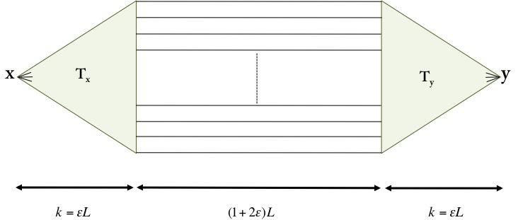
Figure 1: We create for each pair of nodes $x,y$ two node disjoint trees $T_{x},T_{y}$ whose leaves can be matched via a natural isomorphism and linked with edge disjoint paths. For details, see Lemma 2, and [10, 25].

We outline that the events hold with large enough probability. For a detailed proof, please check [27]. The only difference with the proof of Lemma 4 in [27] is that for the first level of trees $T_{x},T_{y}$, we choose $\frac{5\log n}{\delta^{L}}$ neighbors of $x,y$ respectively. For all other levels we use a branching factor equal to $4\log n$. The proof of Theorem 5 follows.

Theorem 5.

Fix a pair of nodes $x,y\in V(G)$, and suppose $x,y$ belong to the same cluster (the other case is treated in the same way). Let $Y_{1},\ldots,Y_{N}$ be the signs of the $N$ edge disjoint paths connecting them, i.e., $Y_{i}\in\{-1,+1\}$ for all $i$. Also let $Y=\sum_{i=1}^{N}Y_{i}$. Notice that $\{Y_{1},\ldots,Y_{N}\}$ is a read-$k$ family where $k=\frac{N}{4\log{n}\delta^{-L}}$. By the linearity of expectation, and Lemma 2 we obtain

$${\mathbb{E}}\left[{Y}\right]=N\delta^{L}\geq n^{\tfrac{4}{5}\epsilon}\delta^{L}.$$

By applying Theorem 4 we obtain

$${\bf{Pr}}\left[{Y<0}\right] ={\bf{Pr}}\left[{Y-{\mathbb{E}}\left[{Y}\right]<-{\mathbb{E}}\left[{Y}\right]}\right]\leq\exp\left(-\frac{n^{4/5\epsilon}\delta^{L}}{\frac{2n^{4/5\epsilon}}{4\delta^{-L}\log{n}}}\right)=o(n^{-2}).$$

A union bound over ${n\choose 2}$ pairs completes the proof. ∎

Algorithm for Learning a Joint Alignment, $k\geq 3$. When $q=0$, so there are no errors from $\tilde{f}(e)$, the edge queries would allow us to determine the difference between the group numbers of vertices at the start and end of any path, and in particular would allow us to determine if the groups were the same. However, when $q>0$ the actual difference between the cluster ids of $x,y$, i.e., $g(x)-g(y)$ is perturbed by a certain amount of noise. In the following we discuss how we can tackle this issue. Since the proof of Theorem 1 overlaps with the proof of Theorem 5 for $k=2$, we outline the main differences. The idea is still the same: among the differences reported by the large number of paths we create between nodes $x,y$, the correct answer $g(x)-g(y)$ will be the plurality vote with large enough probability. The pseudocode is shown in Algorithm 3.

Algorithm 3 Learning Joint Alignment for $k\geq 3$

  $L\leftarrow\frac{\log{n}}{\log{\log{n}}}$

  Perform $20n\log{n}\delta^{-L}$ queries uniformly at random.

  Let $G(V,E,\tilde{f})$ be the resulting graph

  for each item pair $x,y$ do

     $\mathcal{P}_{x,y}=\{P_{1},\ldots,P_{N}\}\leftarrow$ Almost-Edge-Disjoint-Paths($x,y$)

     $Y_{i}(x,y)\leftarrow\sum_{e\in P_{i}}\tilde{f}(e)$ for $i=1,\ldots,N$

     Output the plurality vote among $\{Y_{1}(x,y),\ldots,Y_{N}(x,y)\}$ as the estimate of $g(x)-g(y)$

  end for

Theorem 1.

Let us return to the basic version of our Model, and let $X(e)\in\{-1,0,1\}$ for $e=(x,y)$ be

$$\tilde{f}(e)-(g(x)-g(y))\bmod k.$$

Then given a path between two vertices $x$ and $y$,

$$g(y)=g(x)+\sum_{e\in P_{xy}}\tilde{f}(e)-\sum_{e\in P_{xy}}X(e)\bmod k.$$

Our question is now what is $Z_{xy}=\sum_{e\in P_{xy}}X(e)\bmod k$. We would like that $Z_{xy}$ be (even slightly) more highly concentrated on 0 than on other values, so that when $g(x)=g(y)$, we find that the sum of the return values from our algorithm, $\sum_{e\in P_{xy}}\tilde{f}(e)\bmod k$, is most likely to be 0. We could then conclude by looking over many almost edge-disjoint paths that if this sum is 0 over a plurality of the paths, then $x$ and $y$ are in the same group whp, i.e., the plurality value will equal g(y) - g(x) whp.

For our simple error model, the sum $\sum_{e\in P_{xy}}X(e)\bmod k$ behaves like a simple lazy random walk on the cycle of values modulo $k$, where the probability of remaining in the same state at each step is $q$. Let us consider this Markov chain on the values modulo $k$; we refer to the values as states. Let $p_{ij}^{t}$ be the probability of going from state $i$ to state $j$ after $t$ steps in such a walk. It is well known than one can derive explicit formulas for $p_{ij}^{t}$; see e.g. [8, Chapter XVI.2]. It also follows by simply finding the eigenvalues and eigenvectors of the matrix corresponding to the Markov chain and using that representation. One can check the resulting forms to determine that $p_{0j}^{t}$ is maximized when $j=0$, and to determine the corresponding gap $\max_{j\in[1,k-1]}|p_{00}^{t}-p_{0j}|^{t}$. Based on this gap, we can apply Chernoff-type bounds as in Theorem 4 to show that the plurality of edge-disjoint paths will have error 0, allowing us to determine whether the endpoints of the path $x$ and $y$ are in the same group with high probability.

The simplest example is with $k=3$ groups, where we find

$$p_{00}^{t}=\frac{1}{3}+\frac{2}{3}\left(1-3q/2\right)^{t},$$

and

$$p_{01}^{t}=p_{02}^{t}=\frac{1}{3}-\frac{1}{3}\left(1-3q/2\right)^{t}.$$

In our case $t=L$, and we see that for any $q<2/3$, $p_{00}^{t}$ is large enough that we can detect paths using the same argument as for $k=2$.

For general $k$, we use that the eigenvalues of the matrix

$$\begin{bmatrix}1-q&q/2&0&\dots&q/2\\ q/2&1-q&q/2&\dots&0\\ \vdots&\vdots&\vdots&\vdots&\ddots\\ q/2&0&0&\dots&1-q\end{bmatrix}$$

are $1-q+q\cos(2\pi j/k),j=0,\ldots,k-1$, with the $j$-th corresponding eigenvector being $[1,\omega^{j},\omega^{2j},\ldots,\omega^{j(k-1)}]$ where $\omega=e^{2\pi i/k}$ is a primitive $k$-th root of unity. Here, $i$ is not an index but square root of -1, i.e., $i=\sqrt{-1}$. In this case we have

$$p_{00}^{t}=\frac{1}{k}+\frac{1}{k}\sum_{j=1}^{k-1}\big{(}1-q+q\cos(2\pi j/k)\big{)}^{t}.$$

Note that $p_{00}^{t}>1/k$. Some algebra reveals that the next largest value of $p_{0j}^{t}$ belongs to $p_{01}^{t}$, and equals

$$p_{01}^{t}=\frac{1}{k}+\frac{1}{k}\sum_{j=1}^{k-1}\omega^{-j}\big{(}1-q+q\cos(2\pi j/k)\big{)}^{t}.$$

We therefore see that the error between ends of a path again have the plurality value 0, with a gap of at least

$$p_{00}^{t}-p_{01}^{t}\geq 2(1-\cos(2\pi/k))(1-q+q\cos(2\pi/k))^{t}.$$

This gap is constant for any constant $k\geq 3$ and $q\leq 1/2$. ∎

As we have already mentioned, the same approach could be used for the more general setting where

$$\tilde{f}(e)=g(x)-g(y)+j\text{~{}~{}with probability~{}~{}}q_{j},0\leq j<k,$$

but now one works with the Markov chain matrix

$$\begin{bmatrix}q_{0}&q_{1}&q_{2}&\dots&q_{k-1}\\ q_{k-1}&q_{0}&q_{1}&\dots&q_{k-2}\\ \vdots&\vdots&\vdots&\ddots&\vdots\\ q_{1}&q_{2}&q_{3}&\dots&q_{0}\end{bmatrix}.$$

4 Conclusion

In this work we studied the problem of learning a joint alignment from pairwise differences using a noisy oracle. Based on techniques developed in our previous work [27], we show how we can recover a latent alignment whp using $O(n^{1+o(1)})$ queries. Since the time of the original publication [23], the key open question has been optimally by Larsen and the authors of the paper by providing an optimal (up to constants) non-adaptive algorithm [16]. An interesting open direction is to explore further adaptive algorithms for joint alignment. Finally, developing algorithms for approximate recovery is an interesting open problem.

References

- [1] E. Abbe, A. S. Bandeira, and G. Hall. Exact recovery in the stochastic block model. IEEE Transactions on Information Theory, 62(1):471–487, 2016.
- [2] E. Abbe and C. Sandon. Community detection in general stochastic block models: Fundamental limits and efficient algorithms for recovery. In 56th Annual Symposium on Foundations of Computer Science (FOCS), 2015 IEEE , pages 670–688. IEEE, 2015.
- [3] N. Alon and J. H. Spencer. The probabilistic method. John Wiley & Sons, 2004.
- [4] B. Bollobás. Random graphs. In Modern Graph Theory. Springer, 1998.
- [5] Y. Chen and E. Candés. The projected power method: An efficient algorithm for joint alignment from pairwise differences. arXiv preprint arXiv:1609.05820, 2016.
- [6] A. Dudek, A. M. Frieze, and C. E. Tsourakakis. Rainbow connection of random regular graphs. SIAM Journal on Discrete Mathematics, 29(4):2255–2266, 2015.
- [7] E. Elenberg, K. Shanmugam, M. Borokhovich, A. Dimakis Beyond triangles: A distributed framework for estimating 3-profiles of large graphs. Proceedings of the 21th ACM SIGKDD International Conference on Knowledge Discovery and Data Mining, pages 229-238, 2015
- [8] W. Feller. An introduction to probability theory and its applications: volume I, volume 3. John Wiley & Sons London-New York-Sydney-Toronto, 1968.
- [9] A. Frieze and M. Karoński. Introduction to random graphs. Cambridge University Press, 2015.
- [10] A. Frieze and C. E. Tsourakakis. Rainbow connectivity of sparse random graphs. In Approximation, Randomization, and Combinatorial Optimization (APPROX-RANDOM), pages 541–552. Springer, 2012.
- [11] D. Gavinsky, S. Lovett, M. Saks, and S. Srinivasan. A tail bound for read-k families of functions. Random Structures & Algorithms, 47(1):99–108, 2015.
- [12] B. Hajek, Y. Wu, and J. Xu. Achieving exact cluster recovery threshold via semidefinite programming. IEEE Transactions on Information Theory, 62(5):2788–2797, 2016.
- [13] Q.-X. Huang, H. Su, and L. Guibas. Fine-grained semi-supervised labeling of large shape collections. ACM Transactions on Graphics (TOG), 32(6):190, 2013.
- [14] S. Janson, T. Luczak, and A. Rucinski. Random Graphs, volume 45. John Wiley & Sons, 2011.
- [15] J. H. Kim and V. H. Vu. Concentration of multivariate polynomials and its applications. Combinatorica, 20(3):417–434, 2000.
- [16] K. G. Larsen, M. Mitzenmacher, C. E. Tsourakakis. Optimal Learning of Joint Alignments with a Faulty Oracle. Arxiv:2854757, 2019
- [17] K. G. Larsen, M. Mitzenmacher, C. E. Tsourakakis. Clustering with a faulty oracle Web Conference (WWW) 2020
- [18] J. Leskovec, D. Huttenlocher, and J. Kleinberg. Predicting positive and negative links in online social networks. In Proceedings of the 19th international conference on World Wide Web (WWW), pages 641–650. ACM, 2010.
- [19] A. Mazumdar and B. Saha. Clustering via crowdsourcing. arXiv preprint arXiv:1604.01839, 2016
- [20] A. Mazumdar and B. Saha. Clustering with noisy queries. Advances in Neural Information Processing Systems, pages 5788–5799, 2017.
- [21] C. McDiarmid. Concentration. In Probabilistic methods for algorithmic discrete mathematics, pages 195–248. Springer, 1998.
- [22] F. McSherry. Spectral partitioning of random graphs. In Proceedings. 42nd IEEE Symposium on Foundations of Computer Science (FOCS), pages 529–537. IEEE, 2001.
-
[23]
M. Mitzenmacher, C. E. Tsourakakis.
Joint alignment from pairwise differences with a noisy oracle.
In International Workshop on Algorithms and Models for the Web-Graph (WAW), pages 59–69, 2018, Springer.
For an earlier version, unpublished version see Predicting Signed Edges with Queries, arXiv preprint arXiv:1609.00750, 2016 - [24] A. Perry and A. S. Wein. A semidefinite program for unbalanced multisection in the stochastic block model. In Sampling Theory and Applications (SampTA), 2017 International Conference on, pages 64–67. IEEE, 2017.
- [25] C. E. Tsourakakis. Mathematical and Algorithmic Analysis of Network and Biological Data. arXiv preprint arXiv:1407.0375, 2014
- [26] C. E. Tsourakakis, M. N. Kolountzakis, G.L. Miller. Triangle Sparsifiers. J. Graph Algorithms Appl., pages 703–726, volume 15, 2011
- [27] C. E. Tsourakakis, M. Mitzenmacher, K. G. Larsen, J. Błasiok, B. Lawson, P. Nakkiran, and V. Nakos. Predicting positive and negative links with noisy queries: Theory & practice. arXiv:1709.07308, 2017.
- [28] V. Vu. A simple svd algorithm for finding hidden partitions. arXiv preprint arXiv:1404.3918, 2014.
- [29] L. Wang and A. Singer. Exact and stable recovery of rotations for robust synchronization. Information and Inference: A Journal of the IMA, 2(2):145–193, 2013.
- [30] C. Zach, M. Klopschitz, and M. Pollefeys. Disambiguating visual relations using loop constraints. In Computer Vision and Pattern Recognition (CVPR), 2010 IEEE Conference on, pages 1426–1433. IEEE, 2010.