A magnetar engine for short GRBs and kilonovae

Abstract

We investigate the influence of magnetic fields on the evolution of binary neutron-star (BNS) merger remnants via three-dimensional (3D) dynamical-spacetime general-relativistic (GR) magnetohydrodynamic (MHD) simulations. We evolve a postmerger remnant with an initial poloidal magnetic field, resolve the magnetoturbulence driven by shear flows, and include a microphysical finite-temperature equation of state (EOS). A neutrino leakage scheme that captures the overall energetics and lepton number exchange is also included. We find that turbulence induced by the magnetorotational instability (MRI) in the hypermassive neutron star (HMNS) amplifies magnetic field to beyond magnetar-strength ($10^{15}\,\mathrm{G}$). The ultra-strong toroidal field is able to launch a relativistic jet from the HMNS. We also find a magnetized wind that ejects neutron-rich material with a rate of $\dot{M}_{\mathrm{ej}}\simeq 1\times 10^{-1}\,\mathrm{M_{\odot}\,s^{-1}}$. The total ejecta mass in our simulation is $5\times 10^{-3}\,\mathrm{M_{\odot}}$. This makes the ejecta from the HMNS an important component in BNS mergers and a promising source of $r$-process elements that can power a kilonova. The jet from the HMNS reaches a terminal Lorentz factor of $\sim 5$ in our highest-resolution simulation. The formation of this jet is aided by neutrino-cooling preventing the accretion disk from protruding into the polar region. As neutrino pair-annihilation and radiative processes in the jet (which were not included in the simulations) will boost the Lorentz factor in the jet further, our simulations demonstrate that magnetars formed in BNS mergers are a viable engine for short gamma-ray bursts (sGRBs).

1 Introduction

The inspiral and merger of two neutron star (NSs) are among the loudest and most luminous events in the universe (Abbott et al., 2017a, b). Radioactive material ejected during and after the merger powers a kilonova transient and creates the heaviest elements in the universe (Kasen et al., 2017). Jetted outflows from the merger remnant can launch a sGRB (Ruiz et al., 2016; Goldstein et al., 2017; Savchenko et al., 2017). The multimessenger observations of GW170817 have confirmed our basic understanding of NS mergers (NSMs) (Metzger, 2017) but two key open astrophysics problems for NSMs are how to generate fast-enough outflows to explain the observed blue kilonova component in GW170817 and whether magnetars can launch sGRB jets (Dai & Lu, 1998; Zhang & Mészáros, 2001).

Follow-up of late-time kilonova emission and sGRB radio observations (Mooley et al., 2018; Ghirlanda et al., 2019) have begun to constrain different engine models but no conclusion on the nature of the engine for GRB170817 (i.e. black-hole or magnetar) has been reached.  Metzger et al. (2018) have suggested a magnetar-origin for the blue kilonovae component because hydrodynamic simulations have not been able to produce fast enough outflows (Fahlman & Fernández, 2018). Similarly,  Bucciantini et al. (2012) have shown that magnetars left behind by a NSM are capable of explaining sGRBs, but Numerical Relativity simulations of NSMs have only been able to produce jets after black-hole formation (Ruiz et al., 2016). Simulations leaving behind a stable magnetar have found that baryon pollution of the polar region prevents the launch of a sGRB jet (Ciolfi et al., 2017, 2019; Ciolfi, 2020), but these simulations did not include neutrino effects.

Any merger remnant is likely magnetized by seed fields of the individual NSs and their amplification via Kelvin-Helmholtz instability in the shear layer during the merger (Obergaulinger et al., 2010; Zrake & MacFadyen, 2013; Kiuchi et al., 2015). As a result, magnetic fields play a key role in the postmerger evolution of HMNS. They can launch outflows that eject material along the rotation axis of the remnant (Kiuchi et al., 2012; Siegel et al., 2014) and remove mass and angular momentum. Inside the remnant and in the accretion disk magnetoturbulence can act to redistribute angular momentum and launch winds from the disk surface.

There has been substantial previous work modeling NSMs via MHD simulations, e.g. Price & Rosswog (2006); Duez et al. (2006); Anderson et al. (2008); Rezzolla et al. (2011); Giacomazzo et al. (2011); Dionysopoulou et al. (2013); Neilsen et al. (2014); Palenzuela et al. (2015); Ruiz et al. (2016); Ciolfi et al. (2019); Ruiz et al. (2019); Ciolfi (2020), but these simulations did not employ high-enough resolution to capture the turbulent magnetic field evolution in the merger remnant. Notable exceptions are Kiuchi et al. (2015, 2018) which have performed the highest-resolution GRMHD simulations of NSMs and post-merger evolution to date, but these simulations did not include a realistic nuclear EOS or neutrinos.

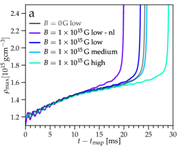
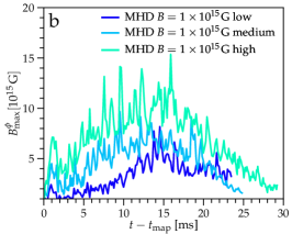
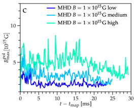
Figure 1: (a) Maximum density as a function of post-mapping time $t-t_{\mathrm{map}}$ for simulations B0 (black), B15-nl (magenta), B15-low (blue), B15-med (cyan), and B15-high (light green). (b) Maximum toroidal magnetic field strength as a function of post-mapping time $t-t_{\mathrm{map}}$ for simulations B15-low (blue), B15-med (cyan), and B15-high (light green). (c) Maximum poloidal magnetic field strength as a function of post-mapping time $t-t_{\mathrm{map}}$ for simulations B15-low (blue), B15-med (cyan), and B15-high (light green).

We perform high-resolution dynamical-spacetime GRMHD simulations of NS merger remnants including a nuclear EOS and neutrino effects. For comparison we also perform simulations which either do not include a magnetic field or do not include neutrino effects. We initialize our simulations by mapping a BNS merger simulation performed in GRHD to a high-resolution domain and add a poloidal magnetic field. We find that MRI-induced turbulence in the HMNS amplifies the magnetic field to beyond magnetar-strength in the HMNS. The added and amplified field launches a relativistic jet from the HMNS in the simulations that include neutrino effects. The emergence of this jet is aided by neutrino cooling reducing baryon pollution in the polar region compared to simulations without neutrino effects. The jet reaches a terminal Lorentz factor of $\sim 5$ in our highest-resolution simulation. In all simulations a magnetized wind driven from the HMNS (Thompson et al., 2004) ejects neutron-rich material with a rate of $\dot{M}_{\mathrm{ej}}\simeq 1\times 10^{-1}\,\mathrm{M_{\odot}\,s^{-1}}$ accounts for the majority of ejected material. The total ejecta mass is $5\times 10^{-3}\,\mathrm{M_{\odot}}$. This makes the ejecta from the HMNS an important component in BNS in addition to the dynamical ejecta and the disk wind once a BH has formed. Our simulations demonstrate that neutrino effects can prevent baryon pollution of the polar region in NSM remnants and that magnetars formed in NS mergers are a viable engine for both sGRBs and kilonova if a large-scale dipolar field can be created.

This paper is organized as follows. In Sec. 2, we present the physical and computational setup and numerical methods used. In Sec. 3.1, we present the simulation dynamics, followed by a description of the jet and ejecta dynamics in Sec. 3.2. We conclude with a discussion of our findings in Sec. 4.

2 Numerical Methods and Setup

We employ ideal GRMHD with adaptive mesh refinement (AMR) and spacetime evolution provided by the open-source Einstein Toolkit  (Babiuc-Hamilton et al., 2019; Löffler et al., 2012; Schnetter et al., 2004; Goodale et al., 2003) module GRHydro (Mösta et al., 2014). GRMHD is implemented in a finite-volume fashion with WENO5 reconstruction (Reisswig et al., 2013; Tchekhovskoy et al., 2007) and the HLLE Riemann solver (Einfeldt, 1988) and constrained transport (Tóth, 2000) for maintaining $\mathrm{div}\vec{B}=0$. We employ the $K_{0}=220\,\mathrm{MeV}$ variant of the equation of state of Lattimer & Swesty (1991) and the neutrino leakage/heating approximations described in O’Connor & Ott (2010) and Ott et al. (2013). The scheme tracks three species: electron neutrinos $\nu_{e}$, electron antineutrinos $\bar{\nu_{e}}$, and heavy-lepton neutrinos which are grouped together into a single species $\nu_{x}$. The scheme approximates neutrino cooling by first computing the energy-averaged neutrino optical depths along radial rays and in a second step calculating local estimates of energy and lepton loss rates. We employ 20 rays in $\theta$, covering $[0,\pi/2]$,and 40 rays in $\phi$ covering $[0,2\pi]$. Each ray has 800 equidistant points to  120 km and 200 logarithmically spaced points covering the remainder of the ray. Neutrino heating is approximated using the neutrino heating rate

$$\mathcal{Q}_{\nu_{i}}^{\mathrm{heat}}=f_{\mathrm{heat}}\frac{L_{\nu_{i}}(r)}{4\pi r^{2}}S_{\nu}\left\langle\epsilon_{\nu_{i}}^{2}\right\rangle\frac{\rho}{m_{n}}X_{i}\left\langle\frac{1}{F_{\nu_{i}}}\right\rangle e^{-2\tau_{\nu_{i}}},$$

where $L_{\nu_{i}}$ is the neutrino luminosity emerging from below as predicted by the neutrino leakage approximation along radial rays, $S_{\nu}=0.25(1+3\alpha^{2})\sigma_{0}(m_{e}c^{2})^{-2}$, $\sigma_{0}=1.76\times 10^{-44}\,\mathrm{cm^{2}}$, $\alpha=1.23$, $m_{e}$ the electron mass, $m_{n}$ the neutron mass, $c$ the speed of light, $\rho$ the rest-mass density, $X_{i}$ the neutron (proton) mass fraction for electron neutrinos (antineutrinos), $\left\langle\epsilon_{\nu_{i}}^{2}\right\rangle$ the mean-squared energy of the $\nu_{i}$ neutrinos, and $\left\langle F_{\nu_{i}}^{-1}\right\rangle$ the mean inverse flux factor. $f_{\mathrm{heat}}$ , the heating scale factor, is a free parameter in this scheme and we set $f_{\mathrm{heat}}=1.05$, consistent with heating in comparison to full neutrino transport schemes in core-collapse supernova simulations (Ott et al., 2013). Further details of the implementation of the scheme can be found in O’Connor & Ott (2010); Ott et al. (2012). We turn neutrino heating off below a density of $\rho=6.18\times 10^{10}\,\mathrm{g\,cm^{-3}}$ for numerical stability. The leakage scheme employed here captures the overall neutrino energetics correctly up to a factor of a few when compared to full transport schemes in core-collapse supernova simulations (O’Connor & Ott, 2010). It does not account for momentum deposition, energy dependence, or neutrino pair annihilation. While the detailed composition of the ejecta depends sensitively on the neutrino scheme we expect the main result of this study, the emergence of a relativistic outflow, to hold.

We map initial data from a GRHD BNS simulation performed with WhiskyTHC, particularly model LS135135M0, an equal-mass binary with individual neutron star masses at infinity $M_{a}=M_{b}=1.35\,M_{\odot}$ and resolution $h\simeq 185\,\mathrm{m}$ covering the merger remnant from Radice et al. (2018). The WhiskyTHC simulation uses the same EOS (LS220) and a very similar but not identical implementation of the neutrino Leakage approximation used in the simulations presented here. We map the HD simulation at $t_{\mathrm{map}}-t_{\mathrm{merger}}=17\,\mathrm{ms}$ and add a magnetic field. The mapping time is chosen to avoid transient effects created by the oscillatory behavior of the remnant core in the early postmerger evolution. We set up the initial magnetic field using a vector potential of the form

$$A_{r}=A_{\theta}=0;A_{\phi}=B_{0}({r_{0}^{3}})({r^{3}+r_{0}^{3}})^{-1}\,r\sin\theta,$$

where $B_{0}$ controls the strength of the field. We choose $r_{0}=20\,\mathrm{km}$ to keep the field nearly constant inside the HMNS. We choose to map this parameterized magnetic field to have full control over our ability to resolve the MRI in the remnant. In doing so we implicitly assume the presence of a dynamo process producing a large scale ordered magnetic field following field amplification during merger. We caution the reader that, while the presence of such dynamo is plausible (Mösta et al., 2015; Raynaud et al., 2020), current simulations do not have sufficient resolution to resolve it (Zrake & MacFadyen, 2013; Kiuchi et al., 2015, 2018).

We perform simulations for initial magnetic field strength $B_{0}=10^{15}\,\mathrm{G}$ (B15-nl, B15-low, B15-med, and B15-high) and a simulation with $B_{0}=0\,\mathrm{G}$ (B0) which acts as a hydrodynamic reference simulation but is performed using the MHD code to keep the numerical methods identical between the simulations. To investigate the influence of neutrino physics we also perform a simulation with magnetic field $B_{0}=10^{15}\,\mathrm{G}$ but without the neutrino leakage scheme enabled (B15-nl). Simulations B0 and B15-nl are performed at the same resolution as B15-low.

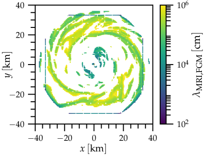
Figure 2: Equatorial slice ($xy$-plane at $z=1.4776\,\mathrm{km}$) of the wavelength of the fastest growing mode of the MRI zoomed in to show the innermost [-40km, 40km] for simulations B15-low at time $t-t_{\mathrm{map}}=0\,\mathrm{ms}$.

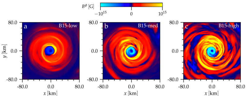
Figure 3: Equatorial slices ($xy$-plane at $z=1.4776\,\mathrm{km}$) of toroidal magnetic field strength $B^{\phi}$ zoomed in to show the innermost [-80km, 80km] for simulations B15-low (panel a), B15-med (panel b), and B15-high (panel c). All panels show the simulations at time $t-t_{\mathrm{map}}=20.9\,\mathrm{ms}$.

We use a domain with outer boundaries $\sim$$355\,\mathrm{km}$ and five AMR levels in a Cartesian grid. The AMR grid structure consists of boxes with extent [$177.3\,\mathrm{km}$, $118.2\,\mathrm{km}$, $59.1\,\mathrm{km}$, $29.6\,\mathrm{km}$]. Refined meshes differ in resolution by factors of 2. We perform simulations at three different resolutions. For our fiducial (low resolution) simulations, the coarsest resolution is $h_{\mathrm{coarse}}=3.55\,\mathrm{km}$ and the level covering the HMNS has $h_{\mathrm{fine}}=220\,\mathrm{m}$. For our medium and high-resolution simulations we use $h_{\mathrm{coarse}}=1.77\,\mathrm{km}$ and $h_{\mathrm{fine}}=110\,\mathrm{m}$, and $h_{\mathrm{coarse}}=0.89\,\mathrm{km}$ and $h_{\mathrm{fine}}=55\,\mathrm{m}$.

We perform simulations in 3D with reflection symmetry in $z$-direction. To prevent numerically-driven oscillations in the magnetic field, we apply diffusivity and hyperdiffusivity at the level of the induction equation for the magnetic field via a modified Ohm’s law. We choose $\vec{E}=-\vec{v}\times\vec{B}+\eta\vec{J}-\eta_{3}\nabla^{3}\times\vec{B}$, where $\vec{J}=\vec{\nabla}\times\vec{B}$ is the 3-current density. In this way the modified Ohm’s law does not impact the ability of the constrained transport scheme to maintain the $\nabla\cdot\vec{B}=0$ constraint. $\Delta x^{i}\,||\nabla\cdot\vec{B}||_{2}/||\vec{B}||_{2}$ in our simulations is $\simeq 6\times 10^{-8}$, $\simeq 8\times 10^{-9}$, and $\simeq 1\times 10^{-9}$ for B15-low, B15-med, and B15-high. We set $\eta=1.0\times 10^{-2}$, $\eta=5.0\times 10^{-3}$, and $\eta=2.5\times 10^{-3}$ for B15-low, B15-med, and B15-high, and $\eta_{3}=3.75\times 10^{-3}$. We estimate the impact of the added diffusivity and hyperdiffusivity terms by studying the time evolution of perturbations of the magnetic field of the form $B_{k}(t)=B_{k}(t=0)\,e^{-k^{2}\eta t}$ for $\eta$ and $B_{k}(t)=B_{k}(t=0)\,e^{-k^{4}\eta_{3}t}$ for $\eta_{3}$. The condition for the diffusivity term not to interfere with numerically resolving the fastest growing mode (FGM) of the MRI can be expressed as $k^{2}\eta<<\frac{1}{\tau_{\mathrm{FGM,MRI}}}$. Using $\tau_{\mathrm{FGM,MRI}}\simeq 0.5\,\mathrm{ms}$, $k=\frac{1}{20h}$ for $\lambda_{\mathrm{FGM,MRI}}\simeq 1000\,\mathrm{m}$ (see Fig. 2), $h=50\,\mathrm{m}$ in B15-high, and expressing $\eta=\alpha h$ in terms of the grid spacing $h$ we can write this condition as $\frac{\alpha}{h}<<4$. For B15-high with $\eta=2.5\times 10^{-3}$ we have $\frac{\alpha}{h}\simeq 0.07$. Following the same procedure we find for the hyperdiffusivity parameter $k^{4}\eta_{3}<<\frac{1}{\tau_{\mathrm{FGM,MRI}}}$ and $\frac{\beta}{h^{3}}<<1600$ with $\eta_{3}=\beta h$. For $\eta_{3}=3.75\times 10^{-3}$ in simulation B15-high we have $\frac{\beta}{h^{3}}\simeq 18$. Thus the diffusivity and hyperdiffusivity terms in our simulations operate on lengthscales significantly smaller than the wavelength of the FGM of the MRI. (Hyper)diffusivity schemes are often employed in high-order numerical simulations of magnetohydrodynamic turbulence, e.g. Brandenburg & Sarson (2002).

Material with density $\rho\leq 10^{4}\,\mathrm{g}\,\mathrm{cm}^{-3}$ in our simulations is considered part of the atmosphere and we set $v^{i}=0$.

3 Results

3.1 Overall dynamics and magnetic field evolution

After mapping from the HD merger simulations to the postmerger MHD simulation domain the added magnetic field in simulations B15-low, B15-med, and B15-high adjusts over a few dynamical times ($t_{\mathrm{dyn,HMNS}}\simeq 0.5\,\mathrm{ms}$ to the underlying hydrodynamical configuration of the remnant and its accretion torus. There is amplification of both poloidal and toroidal magnetic field within the first three milliseconds. A magnetized outflow forms  (Kiuchi et al., 2012; Siegel et al., 2014) and hoop stresses from the windup of strong toroidal field along the rotation axis of the HMNS collimate part of this outflow into a jet. This collimation does not appear in simulation B15-nl and in simulation B0 only a neutrino-driven wind forms. The outflows persist until the HMNS eventually collapses to a BH in all simulations.

Fig. 1 summarizes the overall dynamics of key quantities of the HMNS evolution for simulations B0, B15-nl, B15-low, B15-med, and B15-high. Panel a) shows the central density as a function of time after mapping $t-t_{\mathrm{map}}$. The central density slowly increases as a function of time for all simulations before the HMNS collapses to a BH. BH formation occurs for simulation B15-nl after $\sim 19\,\mathrm{ms}$ and for simulation B0 after $\sim 23\,\mathrm{ms}$. Simulation B15-low collapses $\sim 1\,\mathrm{ms}$ earlier than B0. Simulation B15-med collapses to a BH $\sim 0.5\,\mathrm{ms}$ later than simulation B15-low and B15-high collapses $\sim 6\,\mathrm{ms}$ later.

In Panels b and c we show the maximum toroidal and poloidal magnetic field strength as a function $t-t_{\mathrm{map}}$ for simulations B15-low, B15-med, and B15-high. After an initial nearly-instantaneous adjustment of the magnetic field strength to the hydrodynamic flow, toroidal magnetic field is amplified in all simulations. This growth saturates quickly for simulations B15-low and B15-med but simulation B15-high, which fully resolves the fastest-growing mode of the MRI, reaches a maximum toroidal field of $7\times 10^{15}\,\mathrm{G}$. The amplification happens predominantly in the shear region outside the innermost core the HMNS (see Fig. 3 panel c). In this region the FGM of the MRI has typical wavelengths of 500m - 2000m as shown in Fig. 2. Our highest-resolution simulation B15-high covers this wavelength with 10-40 points. The growth timescale (e-folding time) of $\sim 0.5\,\mathrm{ms}$ approximately matches the rotation period of the HMNS. Subsequently, there is additional amplification of toroidal magnetic in all simulations before the toroidal magnetic field strength decreases after $t-t_{\mathrm{map}}\simeq 15\,\mathrm{ms}$. The poloidal magnetic field is similarly amplified within the first $\sim 2\,\mathrm{ms}$ but subsequently remains in a turbulent state without additional amplification before decreasing slightly in the last few ms before collapse to a BH. In the fully turbulent state secondary instabilities and non-linear effects play an important role and to capture these effects correctly much higher numerical resolution than employed here is needed. For long-term fully sustained turbulence physically complex and numerically difficult to resolve dynamo processes are important. We do not see evidence for these in the simulations presented here indicating that we are not fully resolving the saturated turbulent evolution.

Fig. 3 shows the toroidal magnetic field $B^{\phi}$ in the $xy$-plane at $z=1.4776\,\mathrm{km}$ for simulations B15-low (panel a), B15-med (panel b), and B15-high (panel c) a few ms before collapse to a BH at $t-t_{\mathrm{map}}=20.9\,\mathrm{ms}$. The colormap is chosen such that yellow and light blue indicates magnetar-strength (or stronger) toroidal magnetic field. For simulation B15-low in panel a only a single cylindrical flow region outside the HMNS inner core with magnetar-strength field is visible and barely any small-scale features are present. For simulation B15-med in panel b more magnetar-strength field is visible and small-scale features start to emerge in the region of strong shear outside the inner core of the HMNS $10\,\mathrm{km}<\omega<40\,\mathrm{km}$. For simulation B15-high in panel c the entire inner core and shear region reach magnetar-strength field and small-scale features driven by the magnetorotational turbulence are clearly visible and extend throughout the entire shear region. We note that the inner region of negative toroidal field in all simulations is a result of the positive angular velocity gradient in the inner core.

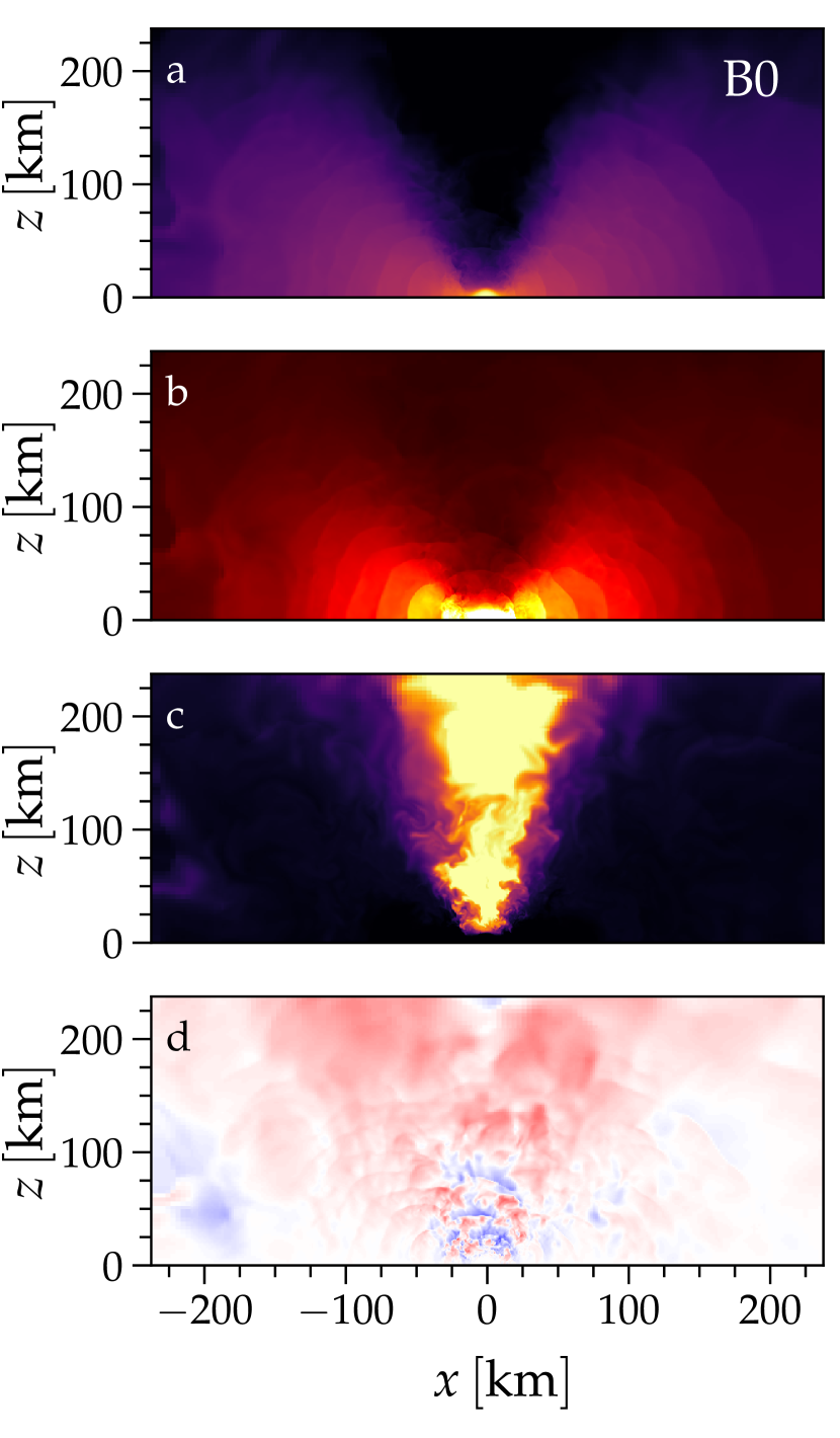
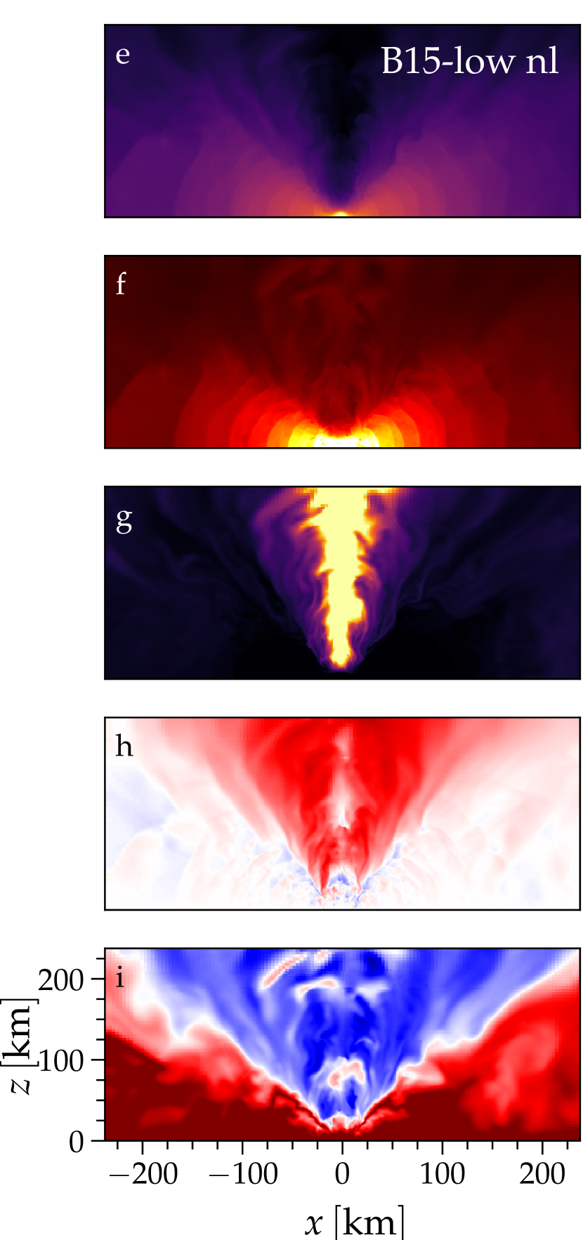
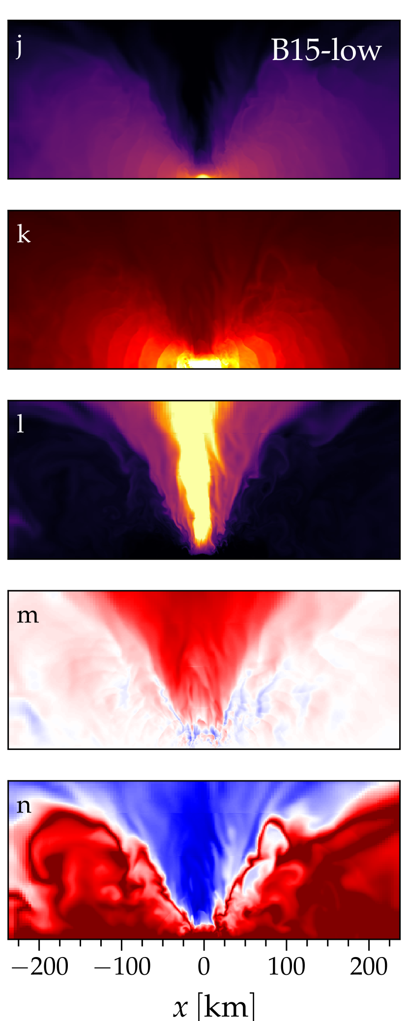
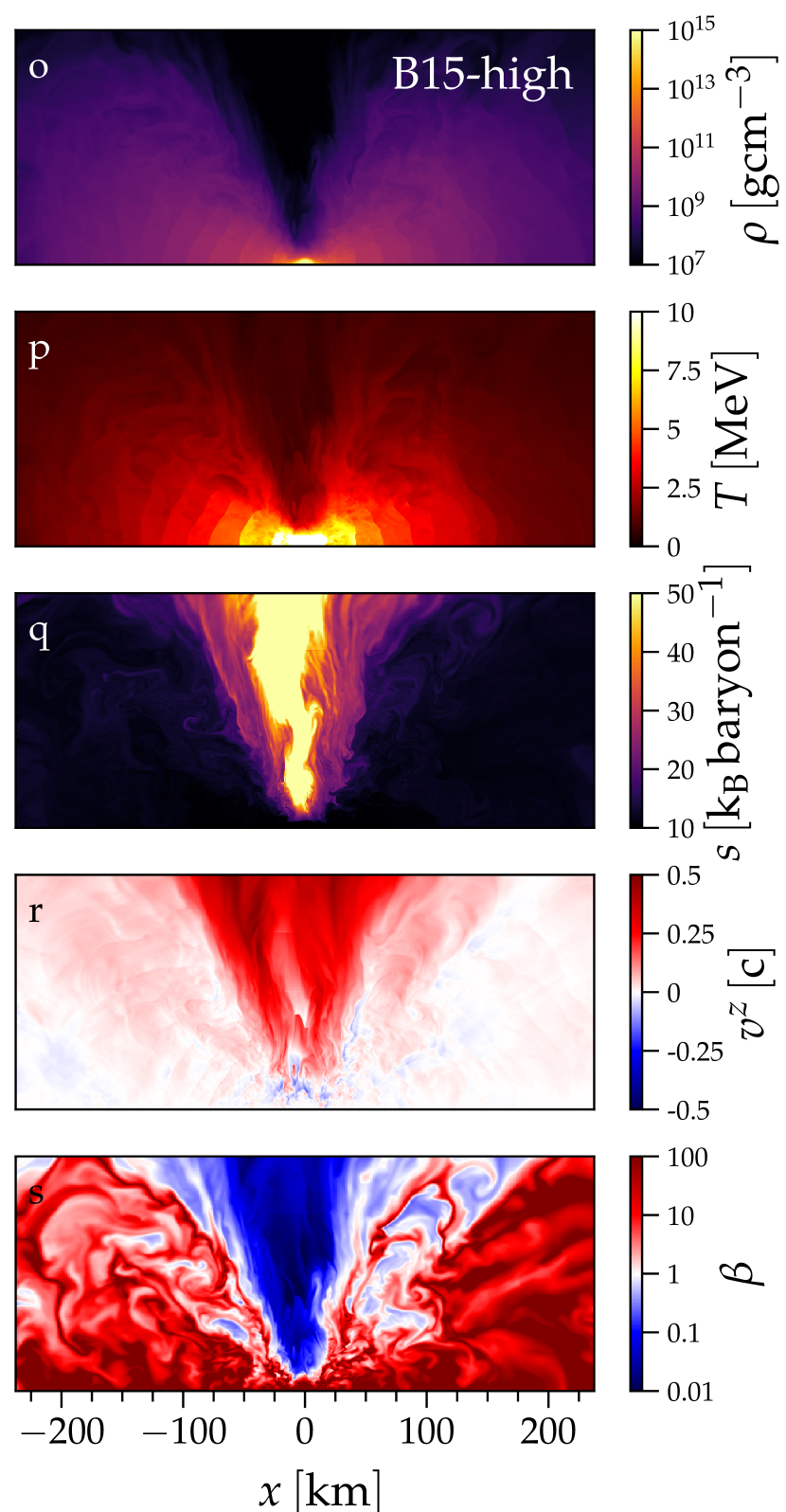
Figure 4: Meridional slices ($xz$-plane, $z$ being the vertical) of density $\rho$, temperature $T$, specific entropy $s$, velocity component aligned with rotation axis $v^{z}$, and magnetic pressure $\beta$. Panels a - d show simulation B0, panels e - i show simulation B15-nl, panels j-n show simulation B15-low, and panels o - s show simulation B15-high (magnetic pressure is only shown for simulations B15-nl, B15-low, and B15-high).

3.2 Outflows

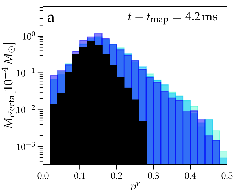
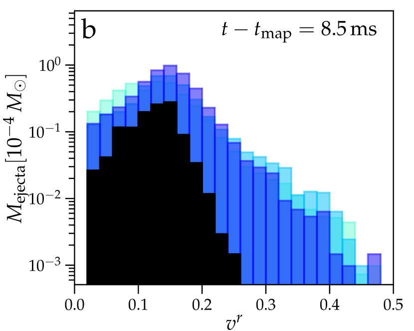
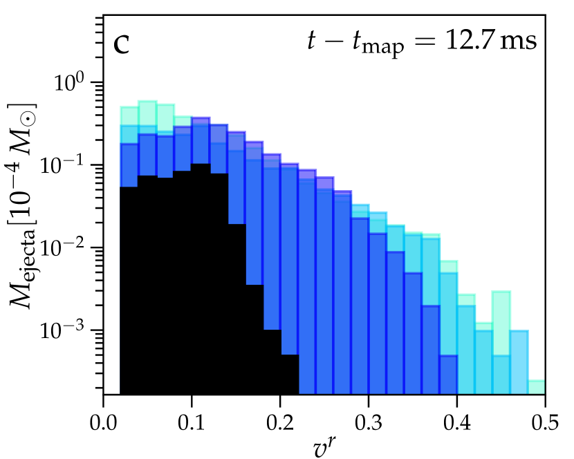
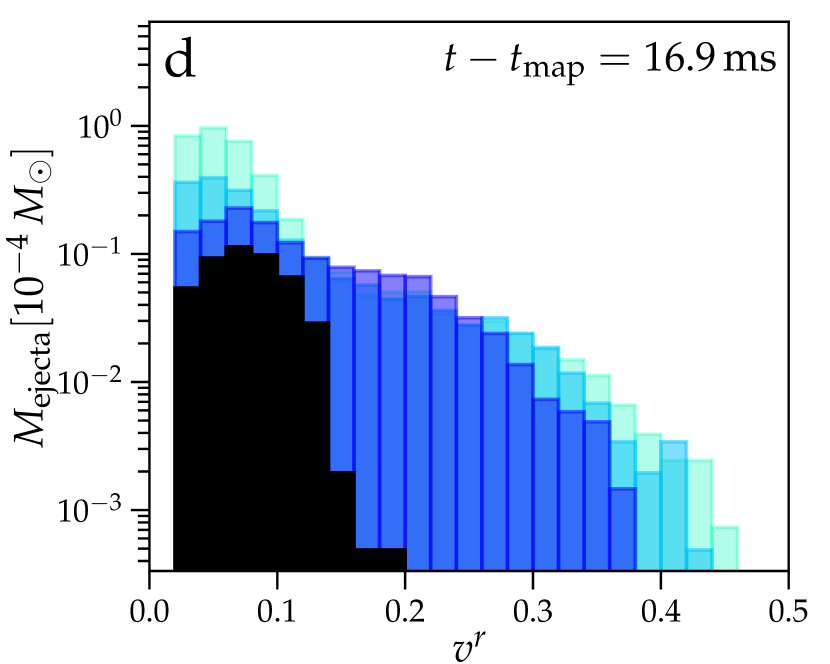
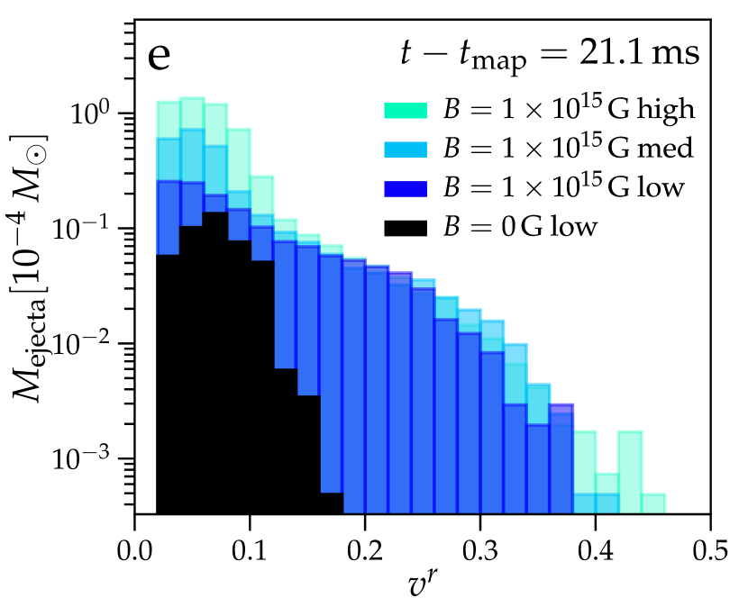
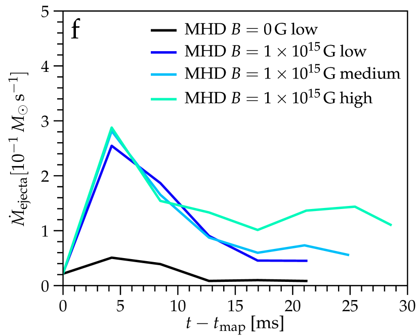
Figure 5: Panels a-e: $v^{r}$ ($r$ being the radius in spherical coordinates) histograms of unbound material at different times during simulations B0 (black), B15-low (blue), B15-med (cyan), and B15-high (green). We bin the distribution with the mass of the ejected material. Panel f: Mass outflow rate $\dot{M}_{\mathrm{ej}}$ as a function of post-mapping time $t-t_{\mathrm{map}}$ for simulations B0 (black), B15-low (blue), B15-med (cyan), and B15-high (light green). We calculate the average (averaged over spheres of $r_{0}<r<r_{1}$) outflow rate as $\dot{M}_{\mathrm{ej}}=\int_{r_{0}}^{r_{1}}\sqrt{g}\rho Wv^{r}dV(r_{1}-r_{0})^{-1}$ with $r_{0}=44.3\,\mathrm{km}$ and $r_{1}=192.1\,\mathrm{km}$ and only include material in the integral if the Bernoulli criterion $-h\,u_{t}>1$ indicates that this material is unbound.

In Fig. 4 we show renderings of density, temperature, specific entropy, z-component of velocity and magnetic pressure in 2D Meridional slices ($xz$-plane, $z$ being the vertical) for simulations B0 (left), B15-nl (center-left), B15-low (center-right), and B15-high (right). We show the renderings at time $t-t_{\mathrm{map}}\simeq 21.2\,\mathrm{ms}$ for simulations B0, B15-low, B15-med, and B15-high, and at $t-t_{\mathrm{map}}\simeq 15.1\,\mathrm{ms}$ for simulation B15-nl to account for the earlier collapse time in simulation B15-nl (see Fig. 1). There are no large differences in density structure of the disk when comparing panels a, e, j, and o. The high-temperature region in the HMNS is more extended for simulation B15-nl compared to simulations B15-low and B15-high (panels f, k, and p). In all our simulations with neutrino effects the polar region remains mostly free of baryon pollution. In contrast simulation B15-nl has a factor 5-10 higher density in the polar region, similarly to the simulations presented in  (Ciolfi et al., 2019; Ciolfi, 2020). The HMNS remains more compact in simulation B15-low and B15-high compared to simulation B15-nl. These differences are in line with neutrino cooling causing the remnant and its accretion disk to stay more compact due to reduced thermal pressure. Key differences between simulation B0 and its magnetized counterparts B15-nl, B15-low, and B15-high arise in the outflow structure. While simulation B0 shows an outflow that resembles a high-entropy wind (panel c), simulations B15-low and B15-high show a collimated, highly magnetized outflow. This is most clearly visible in panels l and q which depict entropy. Simulation B15-nl shows a higher velocity outflow than simulation B0 but lacks a highly collimated component compared to simulations B15-low and B15-high. This is most clearly visible when comparing panels i, n and s which show plasma $\beta=P/b^{2}$. The outflow velocity (panels d,h,m, and r) increases when comparing simulation B0 ($\sim.0.2c$), B15-nl ($\sim.0.3c$), B15-low ($\sim 0.35c$) and B15-high ($\sim 0.45c$).

To analyze the properties and composition of the outflows in more detail we determine unbound material in the simulations via the Bernoulli criterion $-hu_{t}>1$, where $h=(1+\epsilon+P+\frac{b^{2}}{2})/\rho$ is the relativistic enthalpy of the magnetized fluid. We show histograms of $v^{r}$ for the unbound material in Fig. 5. At early times simulations B15-low, B15-med, and B15-high show a similar distribution in velocity of the ejecta and significant material at $0.3c<v^{r}<0.5c$ (panel a). This is in contrast to simulation B0 which only shows ejecta with $0<v^{r}<0.28c$. At later times the velocity distribution of the ejecta shifts slightly for all simulations. For simulation B15 the highest-velocity component of the ejecta ($v^{r}>0.4c$) disappears quickly (panels b - e). Simulation B15-med retains some of this high-velocity ejecta until later times and simulation B15-high retains most of the high-velocity ejecta until late time (panels b - e). In addition all simulations show the appearance of low-velocity material ($v^{r}<0.1c$).

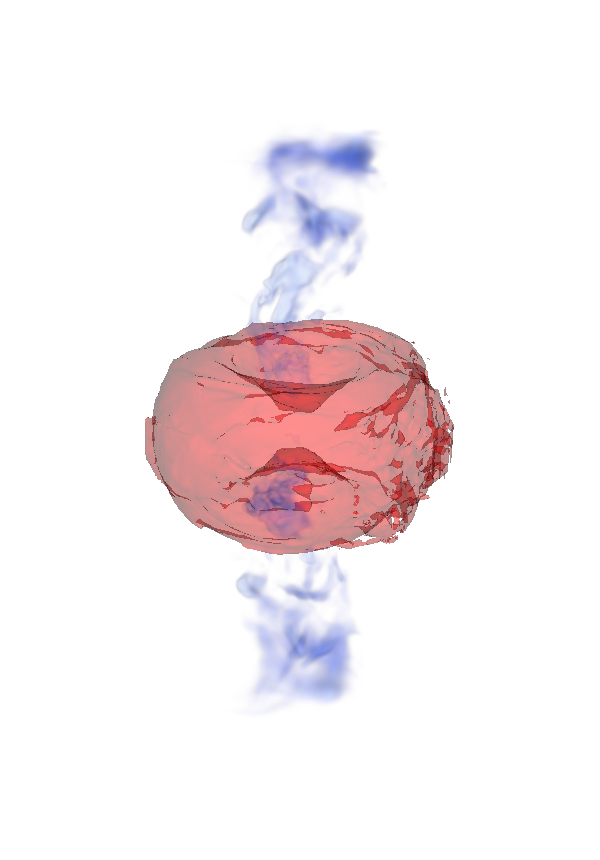
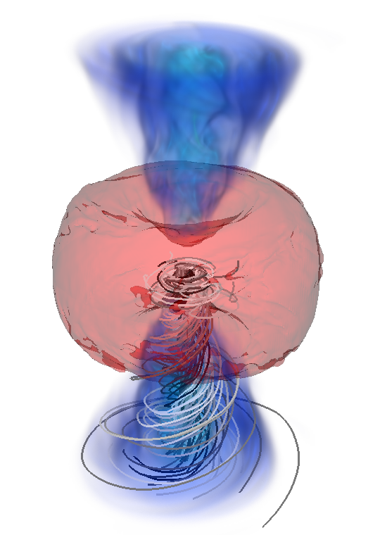
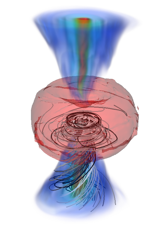
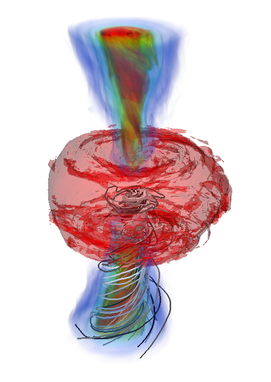
Figure 6: Volume renderings of the Bernoulli criterion (blue colormap) indicating unbound material and the disk contour at $\rho=10^{10}\,\mathrm{g\,cm^{-3}}$ (red) for models B0 (left), B15-nl (center left), model B15-low (center right), and B15-high (right). The renderings depict the simulations at $t-t_{\mathrm{map}}=15.1\,\mathrm{ms}$ for B15-nl, at $t-t_{\mathrm{map}}=19.4\,\mathrm{ms}$ for B0 and B15-low, and at $t-t_{\mathrm{map}}=20.9\,\mathrm{ms}$ for B15-high. The different times are chosen to depict the simulations towards the end of steady-state operation of the outflows which is at different times $t-t_{\mathrm{map}}$ due to the different collapse times (see Fig. 1). Additionally, we show magnetic field lines for simulations B15-nl, B15-low, and B15-high in the lower quadrant of the renderings. The z-axis is the rotation axis of the HMNS and we show the innermost $357\,\mathrm{km}$. The colormap is chosen such that blue corresponds to material with lower Lorentz factors $-h\,u_{t}\simeq 1$, while yellow corresponds to material with $-h\,u_{t}\simeq 1.5$, and red to material with $-h\,u_{t}\simeq 2-5$. We note that for rendering purposes we have excluded part of the unbound ejecta in the equatorial region.

To estimate the outflow rate in the simulations we calculate the averaged mass ejection rate of the outflow $\dot{M}_{\mathrm{ej}}=\int_{r_{0}}^{r_{1}}\sqrt{g}\rho Wv^{r}dV\,(r_{1}-r_{0})^{-1}$ with $r_{0}=44.3\,\mathrm{km}$ and $r_{1}=192.1\,\mathrm{km}$. We only include material in the integral if the material is unbound ($-hu_{t}>1$). We show $\dot{M}_{\mathrm{ej}}$ as a function of post-mapping time $t-t_{\mathrm{map}}$ in panel f of Fig. 5. For all simulations $\dot{M}_{\mathrm{ej}}$ initially rises sharply as the outflow initially forms before reaching a peak at $t-t_{\mathrm{map}}\simeq 5\,\mathrm{ms}$. Subsequently $\dot{M}_{\mathrm{ej}}$ evolves towards a quasi-steady-state that is reached after $t-t_{\mathrm{map}}\simeq 15\,\mathrm{ms}$. The mass ejection rate for simulation B0 in this phase is $\dot{M}_{\mathrm{ej}}=2.4\times 10^{-3}\,\mathrm{M_{\odot}}\ {\rm s}^{-1}$, which are at the very high end compared to the values predicted by Thompson et al. (2001) for a neutrino-driven wind from the HMNS. For simulations B15-low we find $\dot{M}_{\mathrm{ej}}=4.6\times 10^{-2}\ \mathrm{M_{\odot}}\ {\rm s}^{-1}$, for simulation B15-med $\dot{M}_{\mathrm{ej}}=5.6\times 10^{-2}\ \mathrm{M_{\odot}}\ {\rm s}^{-1}$, and finally $\dot{M}_{\mathrm{ej}}=1.2\times 10^{-1}\ \mathrm{M_{\odot}}\ {\rm s}^{-1}$. These outflow rates are a factor $\simeq 20$ (for simulations B15-low and B15-med) and a factor $\simeq 100$ (for simulation B15-high) higher than in the hydrodynamic simulation B0 and are consistent with a magnetized wind (Thompson et al., 2004) from the HMNS.

We can also use $\dot{M}_{\mathrm{ej}}$ to estimate the total ejecta amount for the simulations. For this we average the mass accretion rates over the period of quasi-steady-state evolution and integrate this over the simulation time. We find $M_{\mathrm{ej}}=5.8\times 10^{-5}\,\mathrm{M_{\odot}}$ for simulation B0, $M_{\mathrm{ej}}=1.1\times 10^{-3}\,\mathrm{M_{\odot}}$ for B15-low, $M_{\mathrm{ej}}=1.4\times 10^{-3}\,\mathrm{M_{\odot}}$ for B15-med, and $M_{\mathrm{ej}}=3.5\times 10^{-3}\,\mathrm{M_{\odot}}$ for B15-high. These ejecta masses make the ejecta from the HMNS important when compared to the dynamical ejecta $10^{-4}\,\mathrm{M_{\odot}}<M_{\mathrm{ej}}<10^{-2}\,\mathrm{M_{\odot}}$ and winds driven from a BH accretion disk.

To illustrate the nature and geometry of the outflow, accretion disk, and magnetic field structure we show 3D volume renderings of the Bernoulli criterion in combination with an isocontour plot for a density of $10^{10}\,\mathrm{g\,cm^{-3}}$ and streamlines of the magnetic field for simulations B0, B15-nl, B15-low, and B15-high in Fig. 6. These renderings make the additional emergence of a mildly relativistic jet in simulation B15-low and B15-high immediately obvious (narrow red funnel aligned with rotation axis (z-axis)). This is in contrast to simulation B15-nl. The jet in simulation B15-low reaches a maximum Lorentz factor $\simeq 2$ while the jet in simulation B15-high reaches a Lorentz factor $\simeq 5$. We also calculate the average luminosity of the jet as $L_{\mathrm{ejecta}}=\int_{r0}^{r1}T^{0i}r_{i}dV$ where we include only material in the integral that has $-hu_{t}>2$. During steady-state operation we find $L_{\mathrm{ejecta}}\sim 10^{50}\,\mathrm{erg\,s^{-1}}$ for simulation B15-low and $L_{\mathrm{ejecta}}\sim 10^{51}\,\mathrm{erg\,s^{-1}}$ for simulation B15-high, while simulation B15-nl does not have material with $-hu_{t}>2$. These results indicate that neutrino effects, i.e. neutrino cooling reducing baryon pollution in the polar region, are important for the emergence of the jet and that turbulent magnetic field amplification can significantly boost its Lorentz factor and energetics.

4 Discussion

We have carried out dynamical GRMHD simulations of a magnetized hypermassive NS formed in a BNS merger including a nuclear EOS and neutrino cooling and heating. We have run simulations at three different resolutions of up to $h=55\,\mathrm{m}$ and reference simulations with no magnetic field and no neutrino physics. The highest-resolution simulation is designed to fully resolve magnetoturbulence driven by the MRI. We have run all the simulations to collapse to a BH.

We find an outflow that is consistent with a magnetized wind (Thompson et al., 2004) from the HMNS that ejects neutron-rich material along the rotation axis of the remnant with an outflow rate $\dot{M}_{\mathrm{ej}}\simeq 1\times 10^{-1}\,\mathrm{M_{\odot}\,\mathrm{s^{-1}}}$. This leads to a total ejecta mass of $3.5\times 10^{-3}\,\mathrm{M_{\odot}}$ for the binary configuration we have studied in this paper. We can also use the average outflow rate calculated during quasi-steady state operation to estimate the ejecta mass for binary configurations that leave behind HMNSs that collapse at later times. For longer-lived remnants the total ejecta mass can therefore be the dominant ejecta component when compared to the dynamical ejecta $10^{-4}\,\mathrm{M_{\odot}}<M_{\mathrm{ej}}<10^{-2}\,\mathrm{M_{\odot}}$ and winds driven from a BH accretion disk.

The broad distribution in velocity space of the ejecta with a significant fraction of material with velocities in the range of $0.3c<v^{r}<0.5c$ sets it apart from the dynamical ejecta $v^{r}<0.3c$ and winds driven from an accretion disk $v^{r}<0.1c$ (Fahlman & Fernández, 2018). Thus magnetized winds, possibly in combination with spiral-wave driven outflows (Nedora et al., 2019), can explain the blue component of the kilonova in GW170817, as anticipated by Metzger et al. (2018). Taking into account the outflow rates observed in the simulations, results from other published numerical studies (Shibata et al., 2017; Radice, 2017; Nedora et al., 2019), and the inferred overall mass ejected by the NSM in GW170817, our results suggest a plausible scenario in which the merger remnant collapsed to BH on a timescale of $O(100\ {\rm ms})$. This is consistent with earlier interpretation of the event based on both the red and blue kilonova observations (Margalit & Metzger, 2017).

The magnetic field enables the launch of a jet in all simulations with neutrino effects. The emergence of this jet is aided by neutrino cooling which reduces baryon pollution in the polar region. We also find that MRI-driven turbulence is effective at amplifying the magnetic field in the shear layer outside of the HMNS core to $10^{16}\,\mathrm{G}$ and that this ultra-strong toroidal field can significantly boost the Lorentz factor of the jet. In our highest-resolution simulation the jet reaches a terminal Lorentz factor of $\simeq 5$, is mildly relativistic, and the corresponding luminosity is $\simeq 10^{51}\,\mathrm{erg\,s^{-1}}$. The Lorentz factor measured from our simulations is only a conservative lower estimate as we did not include full neutrino transport. Neutrino pair-annihilation may lead to ejected material being less baryon-rich than in our simulations (Fujibayashi et al., 2017) and this can boost the Lorentz factor to the relativistic sGRB regime (Just et al., 2016). With this in mind our simulations indicate that magnetars formed in NS mergers are a promising sGRB engine.

References

- Abbott et al. (2017a) Abbott, B. P., Abbott, R., Abbott, T. D., et al. 2017a, Physical Review Letters, 119, 161101, doi: 10.1103/PhysRevLett.119.161101
- Abbott et al. (2017b) —. 2017b, ApJ, 848, L12, doi: 10.3847/2041-8213/aa91c9
- Anderson et al. (2008) Anderson, M., Hirschmann, E. W., Lehner, L., et al. 2008, Phys. Rev. Lett., 100, 191101
- Babiuc-Hamilton et al. (2019) Babiuc-Hamilton, M., Brandt, S. R., Diener, P., et al. 2019, The Einstein Toolkit, The ”Mayer” release, ET_2019_10, Zenodo, doi: 10.5281/zenodo.3522086
- Brandenburg & Sarson (2002) Brandenburg, A., & Sarson, G. R. 2002, Phys. Rev. Lett., 88, 055003, doi: 10.1103/PhysRevLett.88.055003
- Bucciantini et al. (2012) Bucciantini, N., Metzger, B. D., Thompson, T. A., & Quataert, E. 2012, MNRAS, 419, 1537, doi: 10.1111/j.1365-2966.2011.19810.x
- Childs et al. (2012) Childs, H., Brugger, E., Whitlock, B., et al. 2012, in High Performance Visualization–Enabling Extreme-Scale Scientific Insight, 357–372
- Ciolfi (2020) Ciolfi, R. 2020, MNRAS, 495, L66, doi: 10.1093/mnrasl/slaa062
- Ciolfi et al. (2017) Ciolfi, R., Kastaun, W., Giacomazzo, B., et al. 2017, Phys. Rev. D, 95, 063016, doi: 10.1103/PhysRevD.95.063016
- Ciolfi et al. (2019) Ciolfi, R., Kastaun, W., Kalinani, J. V., & Giacomazzo, B. 2019, Phys. Rev. D, 100, 023005, doi: 10.1103/PhysRevD.100.023005
- Dai & Lu (1998) Dai, Z. G., & Lu, T. 1998, Phys. Rev. Lett., 81, 4301, doi: 10.1103/PhysRevLett.81.4301
- Dionysopoulou et al. (2013) Dionysopoulou, K., Alic, D., Palenzuela, C., Rezzolla, L., & Giacomazzo, B. 2013, Phys. Rev. D, 88, 044020, doi: 10.1103/PhysRevD.88.044020
- Duez et al. (2006) Duez, M. D., Liu, Y. T., Shapiro, S. L., Shibata, M., & Stephens, B. C. 2006, Phys. Rev. D, 73, 104015
- Einfeldt (1988) Einfeldt, B. 1988, in Shock tubes and waves; Proceedings of the Sixteenth International Symposium, Aachen, Germany, July 26–31, 1987. VCH Verlag, Weinheim, Germany, 671
- Fahlman & Fernández (2018) Fahlman, S., & Fernández, R. 2018, ApJ, 869, L3, doi: 10.3847/2041-8213/aaf1ab
- Fujibayashi et al. (2017) Fujibayashi, S., Sekiguchi, Y., Kiuchi, K., & Shibata, M. 2017, ApJ, 846, 114, doi: 10.3847/1538-4357/aa8039
- Ghirlanda et al. (2019) Ghirlanda, G., Salafia, O. S., Paragi, Z., et al. 2019, Science, 363, 968, doi: 10.1126/science.aau8815
- Giacomazzo et al. (2011) Giacomazzo, B., Rezzolla, L., & Baiotti, L. 2011, Phys. Rev. D, 83, 044014
- Goldstein et al. (2017) Goldstein, A., Veres, P., Burns, E., et al. 2017, ApJ, 848, L14, doi: 10.3847/2041-8213/aa8f41
- Goodale et al. (2003) Goodale, T., Allen, G., Lanfermann, G., et al. 2003, in Vector and Parallel Processing – VECPAR’2002, 5th International Conference, Lecture Notes in Computer Science (Berlin: Springer). http://edoc.mpg.de/3341
- Hunter (2007) Hunter, J. D. 2007, Computing in Science & Engineering, 9, 90, doi: 10.1109/MCSE.2007.55
- Just et al. (2016) Just, O., Obergaulinger, M., Janka, H. T., Bauswein, A., & Schwarz, N. 2016, ApJ, 816, L30, doi: 10.3847/2041-8205/816/2/L30
- Kasen et al. (2017) Kasen, D., Metzger, B., Barnes, J., Quataert, E., & Ramirez-Ruiz, E. 2017, Nature, 551, 80, doi: 10.1038/nature24453
- Kiuchi et al. (2015) Kiuchi, K., Cerdá-Durán, P., Kyutoku, K., Sekiguchi, Y., & Shibata, M. 2015, Phys. Rev. D, 92, 124034, doi: 10.1103/PhysRevD.92.124034
- Kiuchi et al. (2018) Kiuchi, K., Kyutoku, K., Sekiguchi, Y., & Shibata, M. 2018, Phys. Rev. D, 97, 124039, doi: 10.1103/PhysRevD.97.124039
- Kiuchi et al. (2012) Kiuchi, K., Sekiguchi, Y., Kyutoku, K., & Shibata, M. 2012, Class. Quantum Grav., 29, 124003
- Lattimer & Swesty (1991) Lattimer, J. M., & Swesty, F. D. 1991, Nucl. Phys. A, 535, 331, doi: 10.1016/0375-9474(91)90452-C
- Löffler et al. (2012) Löffler, F., Faber, J., Bentivegna, E., et al. 2012, Class. Quantum Grav., 29, 115001, doi: 10.1088/0264-9381/29/11/115001
- Margalit & Metzger (2017) Margalit, B., & Metzger, B. D. 2017, ApJ, 850, L19, doi: 10.3847/2041-8213/aa991c
- Metzger (2017) Metzger, B. D. 2017, arXiv e-prints. https://arxiv.org/abs/1710.05931
- Metzger et al. (2018) Metzger, B. D., Thompson, T. A., & Quataert, E. 2018, ApJ, 856, 101, doi: 10.3847/1538-4357/aab095
- Mooley et al. (2018) Mooley, K. P., Deller, A. T., Gottlieb, O., et al. 2018, Nature, 561, 355, doi: 10.1038/s41586-018-0486-3
- Mösta et al. (2015) Mösta, P., Ott, C. D., Radice, D., et al. 2015, Nature, 528, 376, doi: 10.1038/nature15755
- Mösta et al. (2014) Mösta, P., Mundim, B. C., Faber, J. A., et al. 2014, Class. Quantum Grav., 31, 015005, doi: 10.1088/0264-9381/31/1/015005
- Nedora et al. (2019) Nedora, V., Bernuzzi, S., Radice, D., et al. 2019, ApJ, 886, L30, doi: 10.3847/2041-8213/ab5794
- Neilsen et al. (2014) Neilsen, D., Liebling, S. L., Anderson, M., et al. 2014, Phys. Rev. D, 89, 104029, doi: 10.1103/PhysRevD.89.104029
- Obergaulinger et al. (2010) Obergaulinger, M., Aloy, M. A., & Müller, E. 2010, A&A, 515, A30, doi: 10.1051/0004-6361/200913386
- O’Connor & Ott (2010) O’Connor, E., & Ott, C. D. 2010, Class. Quantum Grav., 27, 114103, doi: 10.1088/0264-9381/27/11/114103
- Ott et al. (2012) Ott, C. D., Abdikamalov, E., O’Connor, E., et al. 2012, Phys. Rev. D, 86, 024026, doi: 10.1103/PhysRevD.86.024026
- Ott et al. (2013) Ott, C. D., Abdikamalov, E., Mösta, P., et al. 2013, ApJ, 768, 115. https://arxiv.org/abs/1210.6674
- Palenzuela et al. (2015) Palenzuela, C., Liebling, S. L., Neilsen, D., et al. 2015, Phys. Rev. D, 92, 044045, doi: 10.1103/PhysRevD.92.044045
- Price & Rosswog (2006) Price, D. J., & Rosswog, S. 2006, Science, 312, 719, doi: 10.1126/science.1125201
- Radice (2017) Radice, D. 2017, ApJ, 838, L2, doi: 10.3847/2041-8213/aa6483
- Radice et al. (2018) Radice, D., Perego, A., Hotokezaka, K., et al. 2018, ApJ, 869, 130, doi: 10.3847/1538-4357/aaf054
- Raynaud et al. (2020) Raynaud, R., Guilet, J., Janka, H.-T., & Gastine, T. 2020, arXiv e-prints, arXiv:2003.06662. https://arxiv.org/abs/2003.06662
- Reisswig et al. (2013) Reisswig, C., Haas, R., Ott, C. D., et al. 2013, Phys. Rev. D., 87, 064023
- Rezzolla et al. (2011) Rezzolla, L., Giacomazzo, B., Baiotti, L., et al. 2011, ApJ, 732, L6
- Ruiz et al. (2016) Ruiz, M., Lang, R. N., Paschalidis, V., & Shapiro, S. L. 2016, ApJ, 824, L6, doi: 10.3847/2041-8205/824/1/L6
- Ruiz et al. (2019) Ruiz, M., Tsokaros, A., Paschalidis, V., & Shapiro, S. L. 2019, Phys. Rev. D, 99, 084032, doi: 10.1103/PhysRevD.99.084032
- Savchenko et al. (2017) Savchenko, V., Ferrigno, C., Kuulkers, E., et al. 2017, ApJ, 848, L15, doi: 10.3847/2041-8213/aa8f94
- Schnetter et al. (2004) Schnetter, E., Hawley, S. H., & Hawke, I. 2004, Class. Quantum Grav., 21, 1465, doi: 10.1088/0264-9381/21/6/014
- Shibata et al. (2017) Shibata, M., Fujibayashi, S., Hotokezaka, K., et al. 2017, Phys. Rev. D, 96, 123012, doi: 10.1103/PhysRevD.96.123012
- Siegel et al. (2014) Siegel, D. M., Ciolfi, R., & Rezzolla, L. 2014, ApJ, 785, L6, doi: 10.1088/2041-8205/785/1/L6
- Tchekhovskoy et al. (2007) Tchekhovskoy, A., McKinney, J. C., & Narayan, R. 2007, MNRAS, 379, 469
- Thompson et al. (2001) Thompson, T. A., Burrows, A., & Meyer, B. S. 2001, ApJ, 562, 887, doi: 10.1086/323861
- Thompson et al. (2004) Thompson, T. A., Chang, P., & Quataert, E. 2004, ApJ, 611, 380, doi: 10.1086/421969
- Tóth (2000) Tóth, G. 2000, J. Comp. Phys., 161, 605
- Zhang & Mészáros (2001) Zhang, B., & Mészáros, P. 2001, ApJ, 552, L35, doi: 10.1086/320255
- Zrake & MacFadyen (2013) Zrake, J., & MacFadyen, A. I. 2013, ApJ, 769, L29, doi: 10.1088/2041-8205/769/2/L29