1 MCMC Convergence Diagnostics

MCMC convergence was assessed by visual examination of trace-plots and by calculating the effective sample sizes (ESS), displayed in this section for the most fire-prone and therefore most representative area, the West region. In Figure 1, we show the ESS and trace-plots for the causal effect estimate at ten randomly selected monitoring sites. The average ESS for the causal effect over all 96 of the monitoring sites was 281.09 (SD=139.649). This was calculated after a burn-in period of 5,000 iterations from 30,000 total iterations; trimming was not included. We also calculated the ESS of the causal effect at the CMAQ centroids (i.e. the Kriging points) was 1,089.7 (SD=950.5). This was computed after a burn-in period of 5,000 iterations; trimming was not included. The ESS for the causal effect estimate at each CMAQ centroid is displayed in Figure 2.

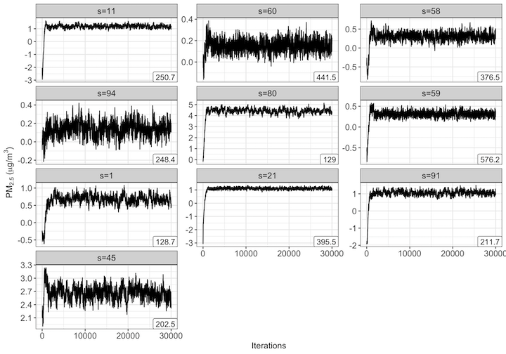
Figure 1: Trace-plots and effective sample size for the causal effect estimates. To monitor MCMC convergence, we visually examined trace-plots and computed the effective sample size (ESS). These plots show the effective sample sizes and trace-plots for the causal effect estimates at ten randomly selected monitoring sites (s) out of the 96 total sites the West Region.

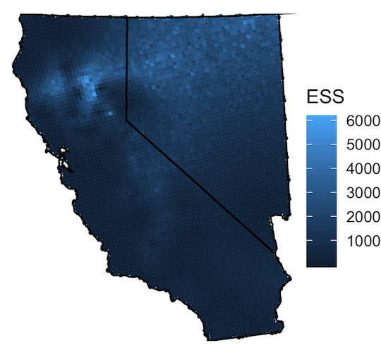
Figure 2: Effective sample sizes for the causal effect estimate at the CMAQ centroids. To monitor MCMC convergence, we computed the effective sample size (ESS) for the causal effect estimates in the West Region. This map shows the effective sample sizes at each CMAQ centroid.

2 Sensitivity to Regional Blocking

We conducted separate analyses for each region of the contiguous U.S. included in our study in order to run our analysis in parallel, thereby speeding up computation. A potential downside of this approach is that correlation between neighboring regions is ignored. Here, we demonstrate that ignoring this correlation has only a small impact.

We conducted a sensitivity test to determine the effects of running separate regional analyses that entailed running the analysis for the Northwest and Western regions as one and compared the resulting causal effect estimates to those from each region run with separate analyses. We chose to focus on the West and Northwest regions since the western US is the most prone to fires. In Figure 3, we display the estimated posterior means and standard deviations of the causal effects for the Northwest and Western regions as one and separately. The resulting spatial patterns are similar, leading us to conclude that our analysis is robust to regional blocking.

Figure 3: Causal effect estimate for the West and Northwest regions separately versus combined. Posterior means (top) and standard deviations (bottom) of the causal effect for the West and Northwest regions as one and separately. We present the $2^{\text{nd}}$, $25^{\text{th}}$, $50^{\text{th}}$, $75^{\text{th}}$, and $98^{\text{th}}$ percentiles of the means and standard deviations.

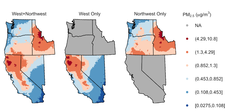
(a) Posterior Mean

(b) Posterior Standard Deviation

3 Spatial Covariance Function

Here, we demonstrate the strength of the correlation between sites. We evaluate

$$\mbox{Cov}[Y_{t}(\mbox{\bf s}),Y_{t}(\mbox{\bf s}^{\prime})|{\hat{\theta}}_{t}(\mbox{\bf s}),{\hat{\delta}}_{t}(\mbox{\bf s})]$$

as defined in Equation (5) in the text, at the posterior mean of the model parameters for each combination of $(C_{t}(\mbox{\bf s}),C_{t}(\mbox{\bf s}^{\prime}))$. Figure 4 displays the plotted covariance functions for each region. The black curve denotes the covariance for observations where neither site is co-located with smoke, the red curve is the covariance for sites where only one is co-located with smoke, and the green curves denote the covariance for two sites co-located with smoke. The strength of the covariance between observations varies between all of the regions, and is strongest in those regularly impacted with wildfire smoke (e.g. West, West North Central).

Figure 4: Spatial covariance functions. The covariance functions from Equation (5) in the text evaluated at the posterior means of the model parameters for each combination of $(C_{t}(\mbox{\bf s}),C_{t}(\mbox{\bf s}^{\prime}))$ at each region.

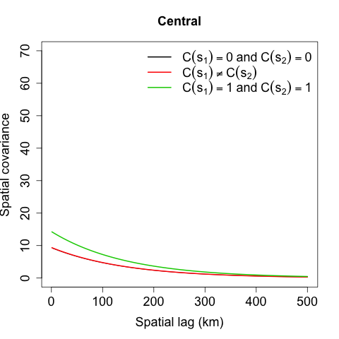
(a) Central

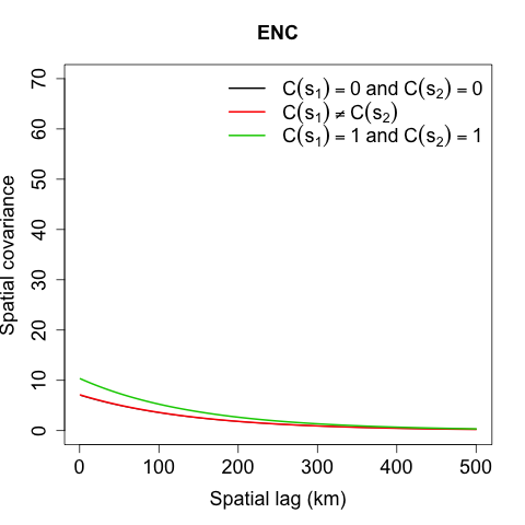
(b) East North Central

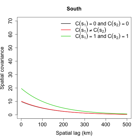
(c) South

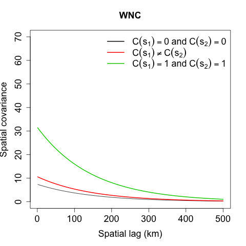
(d) West North Central

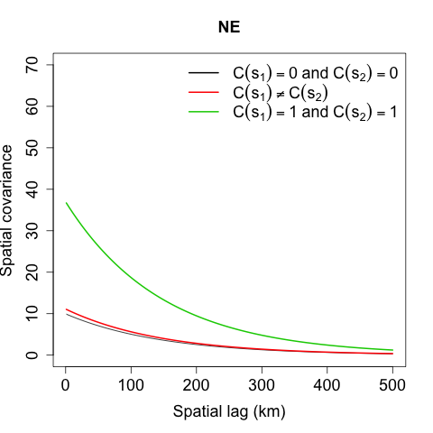
(e) Northeast

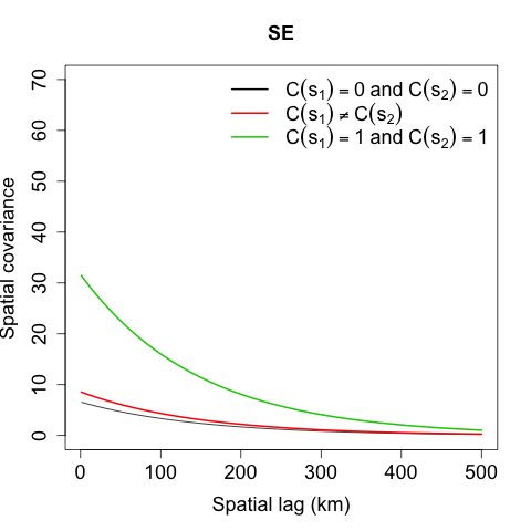
(f) Southeast

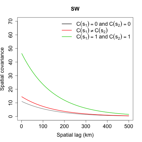
(g) Southwest

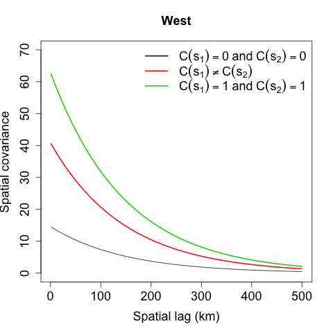
(h) West

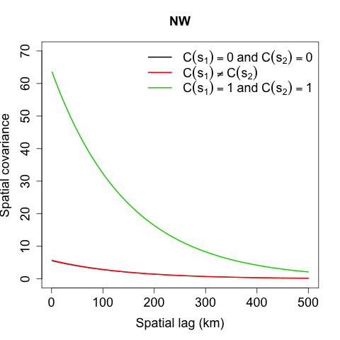
(i) Northwest

4 Sensitivity to $\tau$

In this section, we provide sensitivity analysis to the choice of $\tau$, the smoke presence threshold. In Table 1, we provide results from a cross-validation analysis and in Figure 5 we provide plots of the causal effect estimated under different values of $\tau$ to demonstrate robustness to choice of $\tau$.

Table 1: Five-fold cross-validation results for threshold selection, $\tau$ ($\text{\,}\mathrm{\SIUnitSymbolMicro}\mathrm{g}\mathrm{/}\mathrm{m}^{3}$), using data from California. We report average (over space and time) mean-squared error (MSE), root mean-squared error (RMSE), mean absolute difference (MAD), standard deviation of the predicted values (SD) and coverage of 95% prediction intervals to asses each model’s ability to predict total PM_2.5.

Threshold, $\tau$ ($\text{\,}\mathrm{\SIUnitSymbolMicro}\mathrm{g}\mathrm{/}\mathrm{m}^{3}$)
	$\tau=0$	$\tau=0.1$	$\tau=1$	$\tau=5$	$\tau=10$
MSE	12.59	12.63	12.58	12.71	12.61
RMSE	3.55	3.55	3.55	3.57	3.55
MAD	1.78	1.77	1.78	1.78	1.77
SD	11.84	11.68	11.58	11.47	11.48
Coverage	0.98	0.98	0.98	0.98	0.98

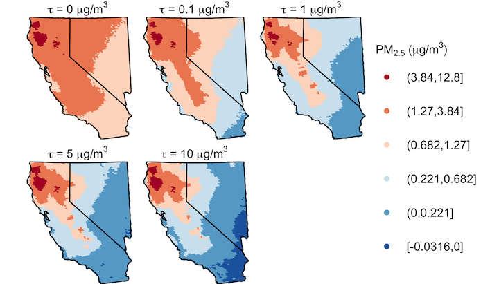
Figure 5: The causal effect given different smoke thresholds. The causal effect estimate is robust to the choice of smoke threshold, $\tau$. This is demonstrated in the maps below, which show the causal effect estimate in the Northwest Region for $\tau=0,0.1,1,5,10$.

5 Residual Autocorrelation

In this section, we present diagnostics to support our assumption of temporal independence between observations. In Figure 6, we plotted residual autocorrelation functions for each region. The residuals are from the linear regression (separate at each site) of the observations $Y_{t}(\mbox{\bf s})$ onto the CMAQ covariates $C_{t}(\mbox{\bf s})$, ${\hat{\theta}}_{t}(\mbox{\bf s})$ and $C_{t}(\mbox{\bf s}){\hat{\delta}}_{t}(\mbox{\bf s})$. We observe that for all of the regions, the lag-one autocorrelation is around 0.2 for most regions.

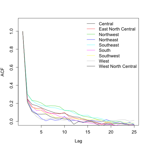
Figure 6: Residual Autocorrelation Function (ACF).

6 Spatial Dependence Model Goodness-of-Fit

We examined variograms of the residuals for each region to determine goodness-of-fit for our spatial dependence model. Figure 7 shows the variograms for all nine regions. We computed the empirical variogram for each combination of $C_{t}(\mbox{\bf s})$, shown in different colors, as well as the variogrom curves evaluated at the posterior means of the covariance parameters, shown as lines.

Figure 7: Spatial variograms.

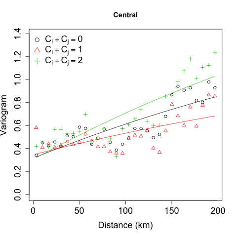
(a) Central

(b) East North Central

(c) Northeast

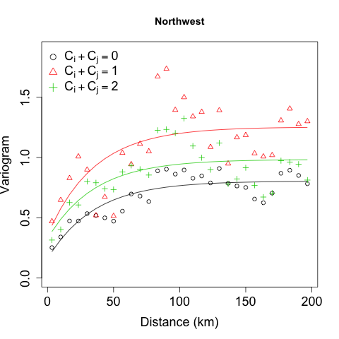
(d) Northwest

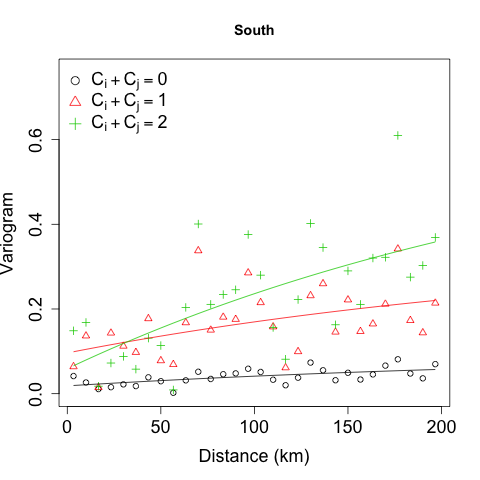
(e) South

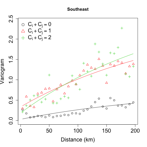
(f) Southeast

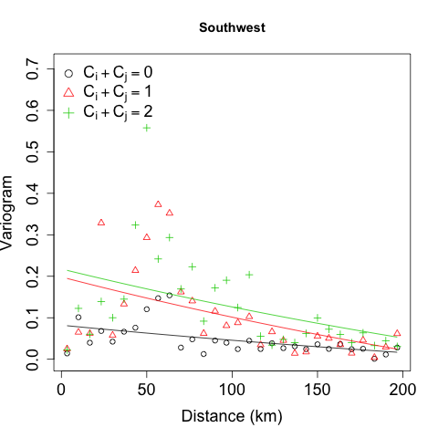
(g) Southwest

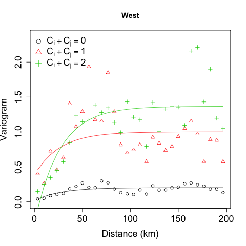
(h) West

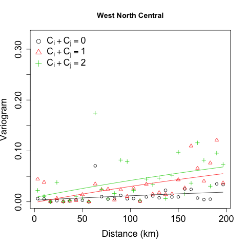
(i) West North Central