Analysis and forecast of COVID-19 spreading in China, Italy and France

Abstract

In this note we analyze the temporal dynamics of the coronavirus disease 2019 outbreak in China, Italy and France in the time window $22/01-11/03/2020$. A first analysis of simple day-lag maps points to some universality in the epidemic spreading, suggesting that simple mean-field models can be meaningfully used to gather a quantitative picture of the epidemic spreading, and notably the height and time of the peak of confirmed infected individuals.
The analysis of the same data within a simple susceptible-infected-recovered-deaths model indicates that the kinetic parameter that describes the rate of recovery seems to be the same, irrespective of the country, while the infection and death rates appear to be more variable. The model places the peak in Italy around March 21^st 2020, with a maximum number of infected individuals of about 15,000 and a number of deaths at the end of the epidemics of about 9,300, consistent with figures typical of seasonal flu epidemics. Since the confirmed cases are believed to be between 10 and 20 % of the real number of individuals who eventually get infected, the apparent mortality rate of COVID-19 falls between 3 % and 7 % in Italy, while it appears substantially lower, between 1 % and 3 % in China.
Based on our calculations, we estimate that $2000$ ventilation units should represent a fair figure for the peak requirement to be considered by health authorities in Italy for their strategic planning. Finally, a simulation of the effects of drastic containment measures on the outbreak in Italy indicates that a reduction of the infection rate indeed causes a quench of the epidemic peak. However, it is also seen that the infection rate needs to be cut down drastically and quickly to observe an appreciable decrease of the epidemic peak and mortality rate. This appears only possible through a concerted and disciplined, albeit painful, effort of the population as a whole.

I Introduction

In December 2019 coronavirus disease 2019 (COVID-19) emerged in Wuhan, China. Despite the drastic, large-scale containment measures promptly implemented by the Chinese government, in a matter of a few weeks the disease had spread well outside China, reaching countries in all parts of the globe. Among the countries hit by the epidemics, Italy found itself grappling with the worst outbreak after the original one, generating considerable turmoil among the population. The exponential increase in people who tested positive to COVID-19 (supposedly together with the sudden increase in the testing rate itself), finally prompted the Italian government to issue on March 8^th 2020 a dramatic decree ordering the lockdown of the entire country.
In this technical note, we report the results of a comparative assessment of the evolution of COVID-19 outbreak in mainland China, Italy and France. Besides shedding light on the dynamics of the epidemic spreading, the practical intent of our analysis is to provide officials with realistic estimates for the time and magnitude of the epidemic peak, i.e. the maximum number of infected individuals, as well as gauge the effects of drastic containment measures based on simple quantitative models. Data were gathered from the github repository associated with the interactive dashboard hosted by the Center for Systems Science and Engineering (CSSE) at Johns Hopkins University, Baltimore, USA Dong et al. (2020). The data analyzed in this study correspond to the period that stretches between January 22^nd 2020 and March 11^th 2020, included.

II Preliminary insight from recurrence plots

A first simple analysis that can be attempted to get some insight into the outbreak dynamics is to build iterative time-lag maps. The idea is to investigate the relation between some population at time (day) $n+k$ and the same population at day $n$, corresponding to a time lag of $k$ days. Of course, the simplest case of all is to build day-by-day maps ($k=1)$. We built three such maps, associated with the population of cumulative confirmed infected people ($C$), recovered people ($R$) and total reported deaths ($D$) for the three countries considered. We note that $I=C-(R+D)$ is the total number of infected individuals, i.e. without taking into accounts recoveries and deaths. Fig. 1 shows that in all cases the data follow the same power law of the kind

$$P_{n+1}=\alpha P_{n}^{\,\beta}$$ (1)

where $\alpha=2.173$ and $\beta=0.928$ and $P=(C,R,D)$. This observation suggests that there is some universality in the epidemic spreading within each country. As a consequence, simple models of the mean-field kind can be adopted to gather a meaningful and quantitative picture of the epidemic spreading in time, to a large extent irrespective of the specific country of interest. In the second part of this note, we provide a concrete example of such an analysis for two of the three countries considered here.
It should be noted that the predicted time evolution of the three populations can be computed analytically from the iterative map (1) (see appendix). More precisely, one has

$$P_{n}=\alpha^{(1-\beta^{n})/(1-\beta)}P_{0}^{\beta^{n}}$$ (2)

where $P=(C,R,D)$. Reassuringly, we find $\beta<1$, which means that the sequence (2) converges to a plateau, which is the (stable) fixed point of the function $F(x)=\alpha x^{\beta}$. Hence, for any value of $P_{0}>0$, one has

$$\lim_{n\to\infty}P_{n}=\alpha^{1/(1-\beta)}$$ (3)

It should be observed that the three populations $C$, $R$ and $D$ are expected to level off at three different values. With respect to Eq. (3), this simply means that one should regard $\beta=0.928$ as an average figure. In fact, each population will be characterized by slightly different value of $\beta$, which will yield considerably different plateaus, since they are all close to the singularity at $\beta=1$ (see again Eq. (3)).

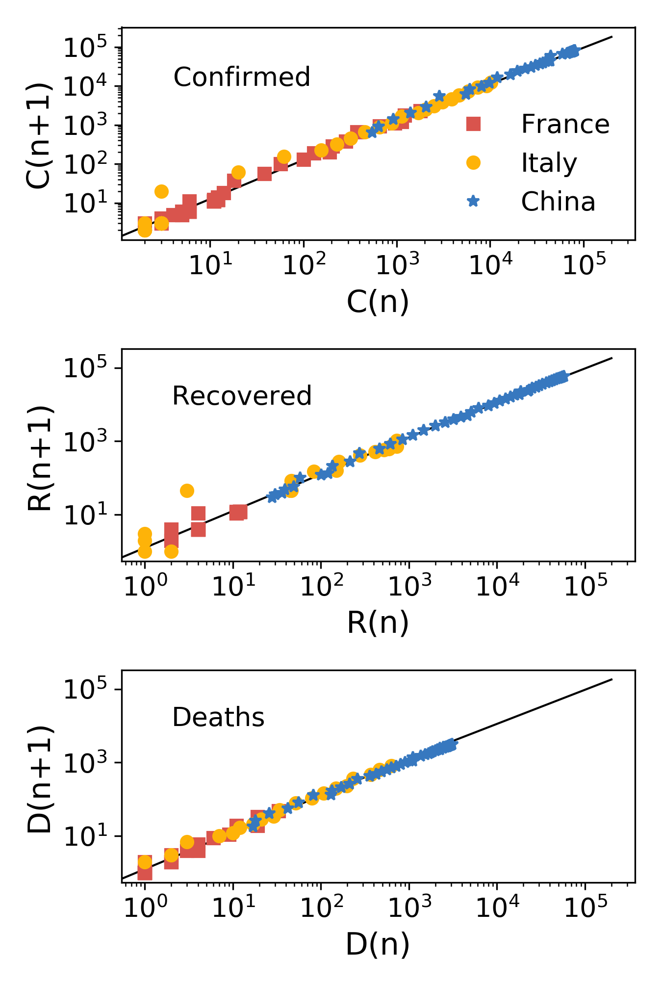
Figure 1: Recurrence plots for the three populations for which data ara publicly available (symbols) for the outbreaks in China, Italy and France and best fit with a power law of the kind (1) (solid lines). All data appear to follow the exact same trend on average (see text).

The prediction (3) should not be regarded as the true asymptotic value to be expected at the end of the outbreak for either populations. Rather, it should be regarded as an estimate of the total population initially within the ensemble of people who will eventually get infected. In fact, the elements of the ensemble $(C,R,D)$ are not independent, as people get infected, recover and die as time goes by, thus effectively transferring elements from one population to another. We will show in the next section how this can be accounted for within a simple kinetic scheme, where eventually such interactions will cause the population of infected individuals $I$ to die out and the $R$ and $D$ populations to reach two separate plateaus as observed. Furthermore, it should be noticed that the data plotted in Fig. 1 start from the first pair of successive values $(P_{n+1},P_{n})$ encountered in the data sheets with $P_{n+1},P_{n}>0$, consistent with the fact that $P=0$ is also a (trivial) fixed point of the map (1).

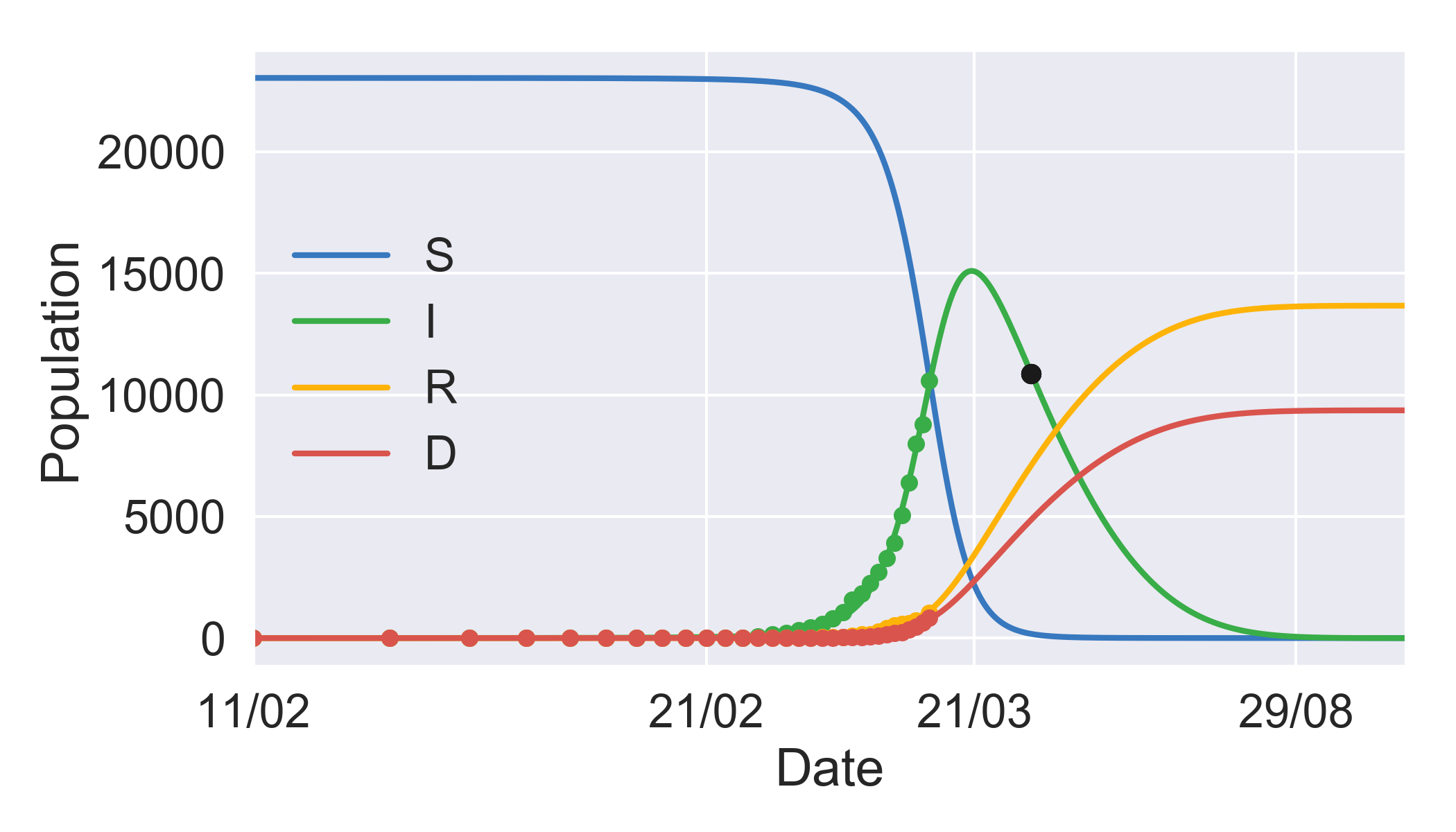
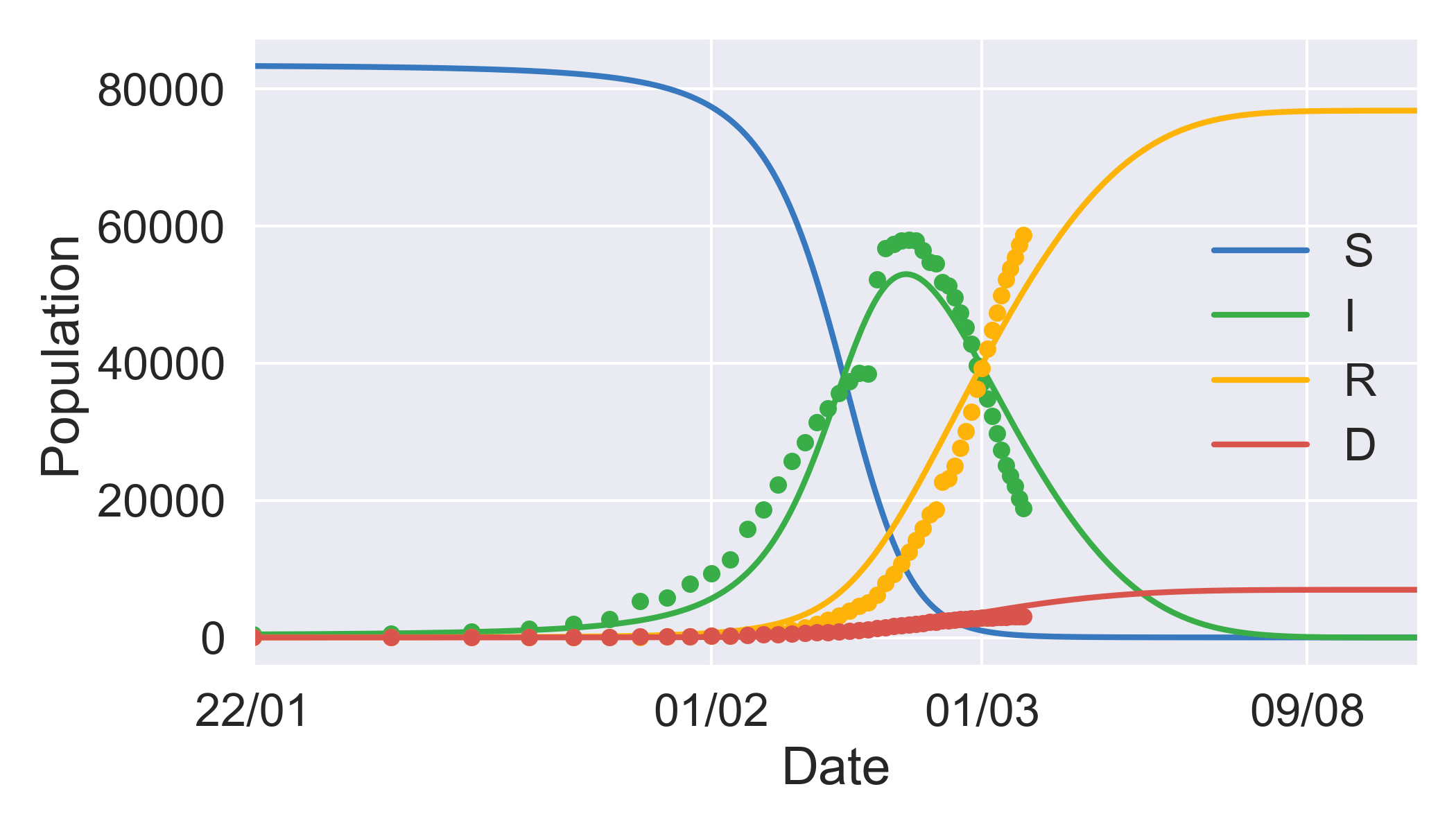
Figure 2: Predicted evolution of the COVID-19 outbreak in Italy (top) and China (bottom). Symbols represent the official data retrieved from the CSSE repository Dong et al. (2020). Solid lines are the predicted trends based on the fits of the SIRD model, Eqs (III), to the data. The black circle in the top graph marks the predicted number of confirmed infected individuals at the announced end of the imposed lockdown on the Italian territory, April 3^rd 2020.

III Mean-field kinetics of the epidemic spreading: exponential growth, peak and decay

As more people get infected, more people also recover or, unfortunately, die. Within the simplest model of the evolution of an epidemic outbreak, people can be divided into different classes (species). In the susceptible (S), infected (I), recovered (R), dead (D) scheme (SIRD), any individual in the fraction of the overall population that will eventually get sick belongs to one of the aforementioned classes. Let $S_{0}$ be the size of the initial population of susceptible people. The mean-field  kinetics of the SIRD epidemic evolution is described by the following system of differential equations

$$\frac{dS}{dt} = -rSI$$

$$\frac{dI}{dt} = rSI-(a+d)I$$

$$\frac{dR}{dt} = aI$$

$$\frac{dD}{dt} = dI$$

with initial condition $[S(t_{0}),I(t_{0}),R(t_{0}),D(t_{0})]=[S_{0},I_{0},R_{0},D_{0}]$ for some initial time $t_{0}$. The parameter $r$ is the infection rate, i.e. the probability per unit time that a susceptible individual contract the disease when entering in contact with an infected person. The parameters $a$ and $d$ denote, respectively, the recovery and death rates. Although the SIRD model is rather crude, the kind of universality emerging from the analysis reported in the previous section for the evolution of non-interacting populations suggests that such scheme has good chances to capture at least the gross features of the full time course of the outbreak.
Fig. 2 illustrates the results of fitting the (numerical) solution of Eqs. (III) simultaneously to the data for the three populations reported in the CSSE sheets, i.e. $I(t),R(t)$ and $D(t)$, for the outbreaks in China and Italy. We found that the data reported for the outbreak in France are still too preliminary to warrant a meaningful fit of this kind. The set of free parameters and the initial conditions used were $[r,a,d,S_{0}]$, $[S_{0},I_{0},0,0]$ in the case of Italy and $[r,a,d,S_{0},R_{0},D_{0}]$, $[S_{0},I_{0},D_{0},R_{0}]$ in the case of China, respectively. In the former case, due to the prolonged initial stretch of stagnancy (presumably due to the initial low testing rate), we chose $t_{0}=20$ days after day one (22/01/2020) and fixed the populations at the corresponding reported values $I_{0}=3,R_{0}=D_{0}=0$. In the case of China, we set $t_{0}$ to day one, as the reported initial populations bear evidence of an outbreak that is already well en route. However, we found that the initial values reported for all the populations, but notably the infected individuals, appear underestimated. This is consistent with the abrupt, visible increase appearing around mid-February, when Chinese authorities changed the testing protocol Dong et al. (2020); WHO . Consequently, we let the initial values $I_{0},S_{0},D_{0}$ float as well during the fits. Interestingly, we found that identical fits could be obtained by fixing the initial values of the populations at the reported values and allowing for a (negative) lag time $\tau$, signifying a shift in the past of the true time origin of the epidemics. In this case, we obtained $\tau=30$ days, consistent with the presumed outset of the outbreak.

Country	$r$ [days-1]		$a$ [days-1]		$d$ [days-1]		$S_{0}$
Italy	$1.460\times 10^{-5}\pm 5\times 10^{-8}$		$2.13\times 10^{-2}\pm 2\times 10^{-4}$		$1.45\times 10^{-2}\pm 2\times 10^{-4}$		$2.303\times 10^{4}\pm 8\times 10^{1}$
China	$3.95\times 10^{-6}\pm 4\times 10^{-8}$		$3.53\times 10^{-2}\pm 1\times 10^{-4}$		$3.1\times 10^{-3}\pm 2\times 10^{-4}$		$8.33\times 10^{4}\pm 2\times 10^{2}$
China∗	$3.33\times 10^{-6}\pm 2\times 10^{-8}$		$1.80\times 10^{-2}\pm 2\times 10^{-4}$		$3.0\times 10^{-3}\pm 2\times 10^{-4}$		$7.92\times 10^{4}\pm 4\times 10^{2}$

Table 1: Table of average values of the best-fit parameters and associated standard deviations computed from 30 independent runs of the stochastic differential evolution algorithm Storn and Price (1997), as implemented in the Python-Scipy package. The line marked with an asterisk refers to a fit limited to the data up to February 19^th 2020.

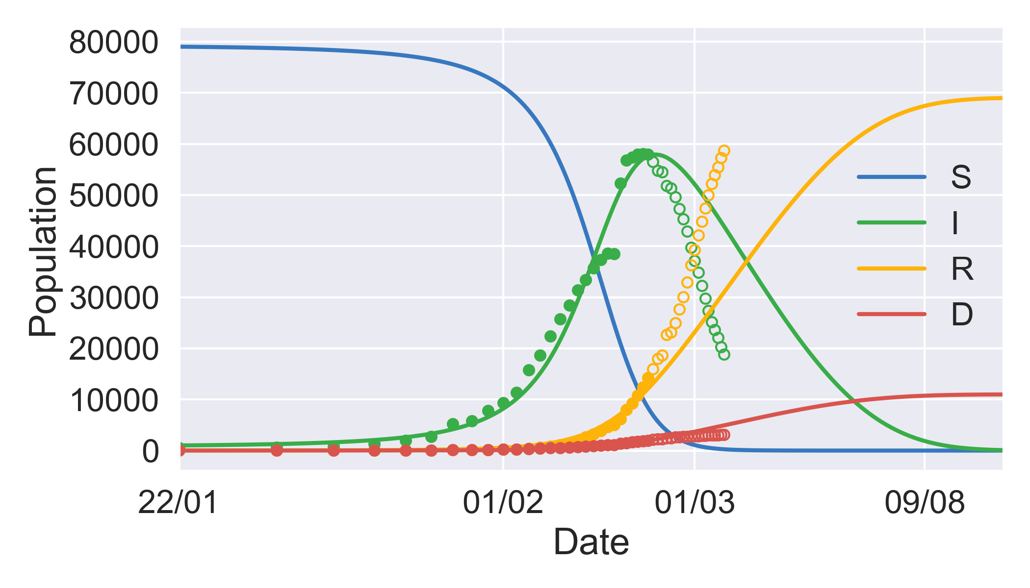
Figure 3: Predicted evolution of the COVID-19 outbreak in China obtained by fitting the data up to to February 19^th 2020. The fitted data are shown as filled circles (see also Table 1). A very similar prediction is obtained by restricting the fit up to February 15^th 2020, where the peak had not been reached yet (data not shown).

The best-fit values of the floating parameters are listed in Table 1. We find that the recovery rate does not seem to depend on the country, while the infection and death rate show a more marked variability. This is likely to be connected with many culture-related habits and to the presumed diversity in underlying health conditions of the more vulnerable that are expected to influence these parameters. It should also be noted that this discrepancy might eventually get reduced when more data on the outbreak in Italy will become available. This would also imply an increase of the initial number of susceptible people, $S_{0}$. However, it turns out that this would entail only a modest shift of the epidemic peak forward in time (data not shown here). The best-fit values of the additional parameters fitted for the China outbreak were $I_{0}=430\pm 20$, $R_{0}=10\pm 10$, $D_{0}=15\pm 7$ (full range) and $I_{0}=999\pm 1$, $R_{0}=10\pm 10$, $D_{0}=17\pm 7$ (full range).
It can be remarked from Fig. 2 that the global fit of the SIRD model, while predicting the observed position of the epidemic peak, it does so at the price of a worse interpolation of the initial growth and of the final decay of the $I$ population. Concurrently, the model fails to follow the observed rapid recovery and overestimates the number of deaths. This is most likely due to the harsh containment measures adopted by the Chinese government in order to curb the spread of the disease. A simple way to test this hypothesis is to restrict the fit to the initial growth phase before the onset of the peak. This is illustrated in Fig. 3. Indeed, it can be appreciated that a model that does not include any external curbing action on the infected population reproduces quite nicely the initial growth phase, places the peak at the correct time, but fails to match the swift recovery rate and decline of the infection in the window where the imposed restrictions are assuredly in action.
The analysis of the outbreak in China strongly suggests that the prediction of our nonlinear fitting strategy for the epidemic peak in Italy is a robust one. However, most likely these data do not bear any signature yet of the harsh, draconian measures contained in the dramatic decree signed by Mr Conte on March 8^th 2020. Equipped with our robust estimates of the kinetic parameters, we are in a good position to inquire whether those measures will impact substantially on the future evolution of the epidemics. To this aim, we consider a modified version of the SIRD model, where the infection rate $r$ is let vary with time. More precisely, given that the containment measures became law at time $t^{\ast}$, we take

$$r(t)=\begin{cases}r_{0}&\text{for}\quad t\leq t^{\ast}\\ r_{0}(1-\alpha)e^{-(t-t^{\ast})/\Delta t}+\alpha\,r_{0}&\text{for}\quad t>t^{\ast}\end{cases}$$ (5)

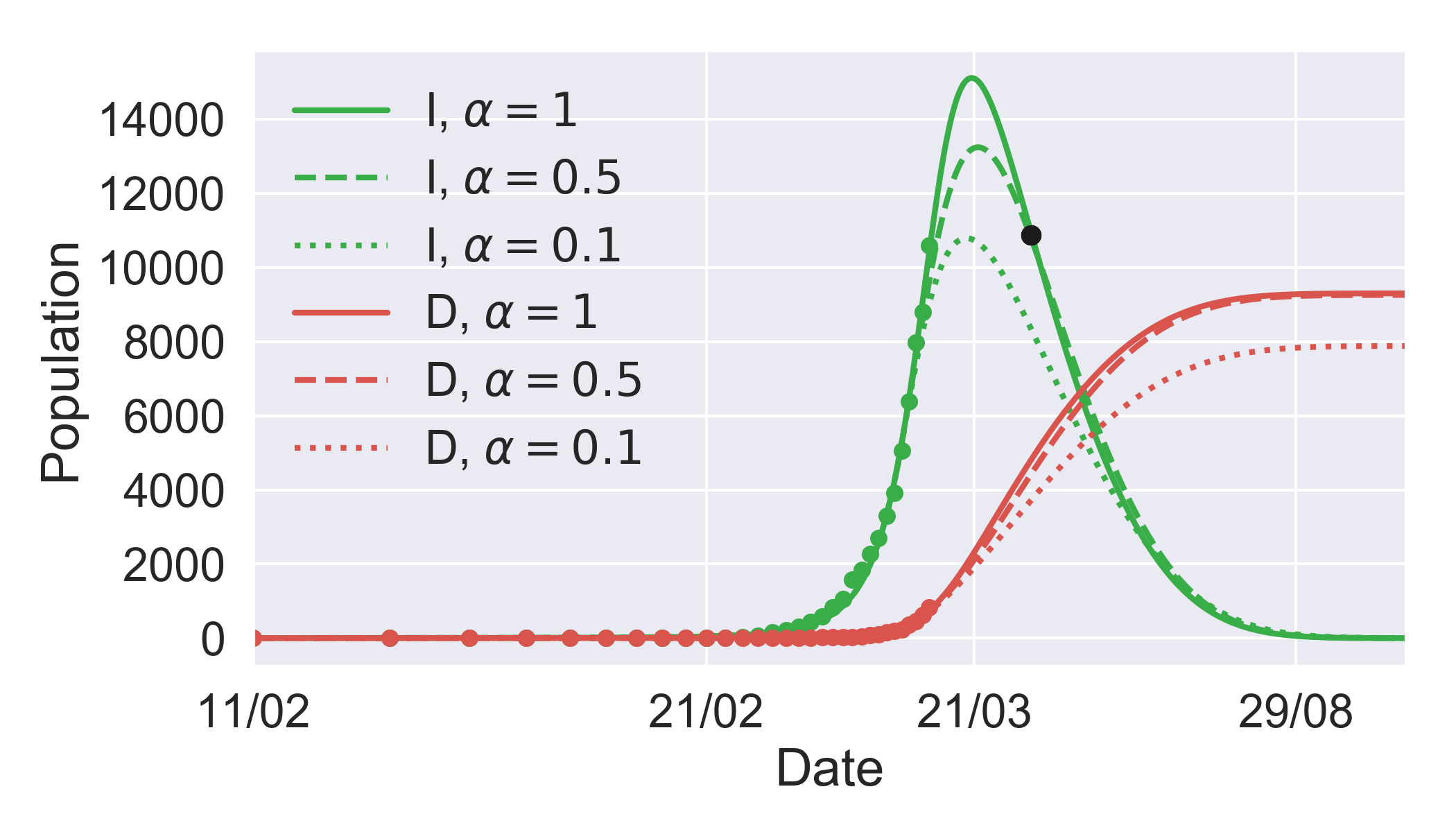
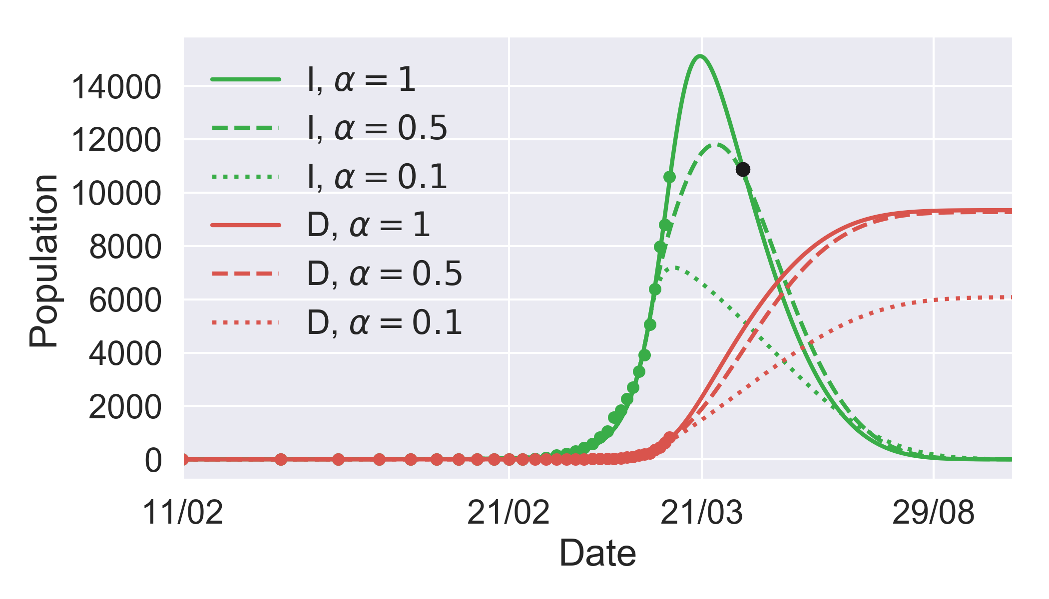
Figure 4: Predicted effect of the lockdown measures imposed by the Italian government on the whole national territory on March 8^th 2020. The predicted evolution of the confirmed infected population and the number of casualties are plotted for different values of the reduction of the infection rate achieved thanks to the lockdown, see Eq. (5). The black circle marks the announced end of the imposed lockdown, April 3^rd 2020. Top graph: $\Delta t=7$ days. Bottom graph: $\Delta t=2$ days.

where $r_{0}=1.46\times 10^{-5}$ days^-1 is the rate estimated from the fit to the data shown in Fig. 2, hence unaffected by the lockdown, and $\alpha\in[0,1]$ gauges the asymptotic reduction of the infection rate afforded by the containment measures. Fig. 4 shows two predictions based on such modified SIRD model, for intermediate (50 %) and large (90 %) reduction of the infection rate, with $t^{\ast}$ fixed at the date of the signature of the decree and $\Delta t$ = 7 and 2 days, i.e. assuming that the effects of the lockdown will be visible on a time of the order of one week or a few days.
It can be appreciated that the effect is predicted to be the one the government was hoping for. Moreover, it can be seen that the quickest the drop in the infection rate brought about by the containment measures, the more substantial the reduction of the epidemic peak. However, it can also be seen that the infection rate should be cut down rather drastically for the measures to be effective. Overall, the dynamics of the decay of the epidemics after the peak and the mortality rate seem also little affected by a time decay of the infection rate, unless this happens very quickly (in a matter of days) and suppressing new infections by at least 90 %.

IV Discussion

In this report we have analyzed epidemic data made available to the scientific community by the Center for Systems Science and Engineering at Johns Hopkins University Dong et al. (2020) and referring to the period $22/02/2020-11/03/2020$. Our results seem to suggest that there is a certain universality in the time evolution of COVID-19. This is demonstrated by time-lag plots of the confirmed infected populations of China, Italy and France, which collapse on one and the same power law on average. This suggests that a country that becomes the theatre of an epidemics surge can be regarded, at least in first approximation, as a well-stirred chemical reactor, where different populations interact according to mass-action-like rules with little connection to geographical variations.
The analysis of the same data within a simple susceptible-infected-recovered-deaths (SIRD) model reveals that the recovery rate is the same for Italy and China, while infection and death rate appear to be different. A few observations are in order. Chinese authorities have tackled the outbreak by imposing martial law to a large fraction on the population, thus presumably cutting down the infection rate to a large extent. While data on the outbreak in China bear the signature of this measure, the data on the outbreak in Italy clearly do not at this stage. Moreover, it can be surmised that many cultural factors could influence the infection rate, thus leading to a larger variability from one country to another. Analysis of data from more than two countries of course are needed to substantiate this hypothesis. The death rate probably reflects the average age and underlying health conditions of elderly patients, which are also likely to vary markedly depending on culture and lifestyle.
As more data will become available for the outbreak in France, the same analysis will be attempted on those data too. In fact, the outbreak appears to have started later in France than in Italy. However, the confirmed cases reported could be biased by a non-stationary testing rate, which could have increased substantially after the severity of the outbreak in Italy came under the spotlight. This document will be updated regularly during the outbreak, and predictions of the peak time and severity in France will be included as soon as the data will make these calculations meaningful.
The SIRD model places the peak in Italy around March 21^st 2020, and predicts a maximum number of confirmed infected individuals of about 15,000 at the peak of the outbreak. The number of deaths at the end of the epidemics appear to be about 9,300, which is consistent with figures typical of seasonal flu epidemics. Taking into account that the confirmed cases can be estimated to be between 10 and 20 % of the real number of infected individuals WHO , the apparent mortality rate of COVID-19 seems to be between 3 % and 7 % in Italy, higher than seasonal flu, while it appears substantially lower in China, that is, between 1 % and 3 %.
Furthermore, assuming that the fraction of sick people needing intensive care with ventilation appears to be about $5-10$ % of those who contract the disease Guan et al. (2020), the maximum number of individual ventilation units required overall to handle the epidemic peak in Italy, i.e around 15,000 cases, can be estimated to be around $1000-1500$. We believe that a more conservative estimate of 2000 ventilation units as the peak requirement represents a fair figure to be handled to the health authorities for their strategic planning.
Finally, based on the kinetic parameters fitted on the data for the outbreak in Italy, i.e. up to the day following the painful lockdown of the whole nation enforced on March 8^th 2020, we have computed the prediction of the SIRD model modified by the highly awaited effects of a fading infectivity following the lockdown. While a reduction in the epidemic peak and mortality rate are indeed observed, we predict that such effects will only be visible if the measures cause a quick (matter of days) and drastic (down by at least $80-90$ %) cutback of the infection rate. In Italy and in other countries that will be facing the epidemic surge soon, this is quite possibly only achievable through a cooperative and disciplined effort of the population as a whole.

This note is available as an ongoing project on ResearchGate at the following address:
https://www.researchgate.net/project/Analysis-and-forecast-of-COVID-19-spreading-in-China-and-Europe The analyses presented in this report will be updated regularly during the course of the global outbreak and extended to other countries. The authors hope that this project will be of some help to health and political authorities during the difficult moments of this global outbreak.

Appendix A Calculation of the explicit form of the iterative map

From Eq. (1) one can determine the explicit form of the population $P_{n}$ at time $n$ (P=C,R,D). The steps of the iteration can be worked out explicitly, that is,

$$P_{1} = \alpha P_{0}^{\,\beta}$$

$$P_{2} = \alpha P_{1}^{\,\beta}=\alpha^{1+\beta}P_{0}^{\,\beta^{2}}$$

$$\dots$$

$$P_{n} = \alpha^{1+\beta+\beta^{2}\dots\beta^{n-1}}P_{0}^{\beta^{n}}$$

Recalling that

$$1+\beta+\beta^{2}\dots+\beta^{n-1}=\frac{1-\beta^{n}}{1-\beta}$$ (6)

one eventually gets Eq. (2).

References

- Dong et al. (2020) E. Dong, H. Du, and L. Gardner, The Lancet Infectious Diseases 3099, 19 (2020).
- (2) URL https://www.who.int/emergencies/diseases/novel-coronavirus-2019/situation-reports/.
- Storn and Price (1997) R. Storn and K. Price, Journal of Global Optimization 11, 341 (1997).
- Guan et al. (2020) W.-j. Guan, Z.-y. Ni, Y. Hu, W.-H. Liang, C.-q. Ou, J.-x. He, L. Liu, H. Shan, C.-l. Lei, D. S. C. Hui, et al., The New England journal of medicine p. 10.1056/NEJMoa2002032 (2020).