Exploring the Limits of Open Quantum Dynamics I: Motivation, New Results from Toy Models to Applications

Abstract

Which quantum states can be reached by controlling open Markovian $n$-level quantum systems? Here, we address reachable sets of coherently controllable quantum systems with switchable coupling to a thermal bath of temperature $T$. — The core problem reduces to a toy model of studying points in the standard simplex allowing for two types of controls: (i) permutations within the simplex, (ii) contractions by a dissipative semigroup [Dirr et al. (2019)]. By illustration, we put the problem into context and show how toy-model solutions pertain to the reachable set of the original controlled Markovian quantum system. Beyond the case $T=0$ (amplitude damping) we present new results for $0<T<\infty$ using methods of $d$-majorisation.

final version: 26 May 2020

1 Introduction

Here we show how reachability problems of (finite dimensional) Markovian open quantum systems may reduce to hybrid control systems on the standard simplex of $\mathbb{R}^{n}$. Consider a bilinear control system [Jurdjevic (1997); Elliott (2009)]

$$\dot{\mathbf{x}}(t)=-(A+\sum\nolimits_{j}u_{j}(t)B_{j})\mathbf{x}(t)\,,\quad\mathbf{x}(0)=\mathbf{x}_{0}\,,$$ (1)

where as usual $A$ denotes an uncontrolled drift, while the control terms consist of (piecewise constant) control amplitudes $u_{j}(t)\in\mathbb{R}$ and control operators $B_{j}$. The state $\mathbf{x}(t)$ may be thought of as (vectorized) density operator. The corresponding system Lie algebra, which provides the crucial tool for analysing controllability and accessibility questions, reads $\mathfrak{k}:=\langle A,B_{j}\,|\,j=0,1,\dots,m\rangle{}_{\sf Lie}$.

For ‘closed’ quantum systems, i.e. systems which do not interact with their environment, the matrices $A$ and $B_{j}$ involved are skew-hermitian and thus it is known [Jurdjevic and Sussmann (1972); Brockett (1972); Jurdjevic (1997)] that the reachable set of (1) is given by the orbit of the initial state under the action of the dynamical systems group $\mathbf{K}:=\langle\exp\mathfrak{k}\rangle{}$, provided $\mathbf{K}$ is a closed and thus compact subgroup of the unitary group.

More generally, for ‘open’ systems undergoing Markovian dissipation, the reachable set takes the form of a (Lie) semigroup orbit, see, e.g., [Dirr et al. (2009)]. – Here we address a scenario with coherent controls $\{B_{j}\}_{j=1}^{m}$ and a bang-bang switchable dissipator $B_{0}$, the latter being motivated by recent experimental progress [Chen et al. (2014); Wong et al. (2019)] as described in Bergholm et al. (2016).

Specification of the Toy Model — These assumptions and the condition that $B_{0}$ leaves the set of diagonal matrices invariant simplify the reachability analysis of (1) to the core problem of diagonal states represented by probability vectors of the standard simplex

$$\Delta^{n-1}:=\big{\{}x\in\mathbb{R}_{+}^{n}\,|\,{\textstyle\sum}_{i=1}^{n}x_{i}=1\big{\}}\,,$$ (2)

i.e. $\mathbf{x}(t)=\operatorname{diag}(x(t))$. In order to make the main features match the quantum dynamical context, let us fix the following stipulations for the toy model: Its controls shall amount to permutation matrices acting instantaneously on the entries of $x(t)$ and a continuous-time one-parameter semigroup $(e^{-tB_{0}})_{t\in\mathbb{R}^{+}}$ of stochastic maps with a unique fixed point $d$ in $\Delta^{n-1}$. As $(e^{-tB_{0}})_{t\in\mathbb{R}^{+}}$ results from the restriction of the bang-bang switchable dissipator $B_{0}$, with abuse of notation we will denote its infinitesimal generator again by $B_{0}$. The ‘equilibrium state’ $d$ is defined in (8) by system parameters and the absolute temperature $T\geq 0$ of an external bath.

These stipulations suggest the following hybrid/impulsive scenario to define the ‘toy model’ $\Lambda$ on $\Delta^{n-1}\subset\mathbb{R}^{n}$ by

$$\begin{split}&\dot{x}(t)=-B_{0}x(t)\,,\quad x(t_{k})=\pi_{k}x_{k}\,,\quad t\in[t_{k},t_{k+1})\,,\\ &x_{0}\in\Delta^{n-1}\,,\quad x_{k+1}=e^{-(t_{k+1}-t_{k})B_{0}}x(t_{k})\,,\quad k\geq 0\,.\end{split}$$ (3)

Furthermore, $0=:t_{0}\leq t_{1}\leq t_{2}\leq\dots$ is an arbitrary switching sequence and $\pi_{k}$ are arbitrary permutation matrices. Both the switching points and the permutation matrices are regarded as controls for (3). For simplicity, we assume that the switching points do not accumulate on finite intervals. For more details on hybrid/impulsive control systems see, e.g., [Lakshmikantham et al. (1989); Alur et al. (1996)]. The reachable sets of (3)

$$\mathfrak{reach}_{\Lambda}(x_{0}):=\{x(t)\,|\,\text{$x(\cdot)$ is a solution of \eqref{eq:control-simplex_evolution}, $t\geq 0$}\}$$

allow for the characterisation $\mathfrak{reach}_{\Lambda}(x_{0})={\mathcal{S}}_{\Lambda}x_{0}\,,$ where ${\mathcal{S}}_{\Lambda}\subset\mathbf{GL}(n,\mathbb{R})$ is the contraction semigroup generated by $(e^{-tB_{0}})_{t\in\mathbb{R}_{+}}$ and the set of all permutation matrices $\pi$.

2 State-of-the-Art

Henceforth, let $\mathbf{\Gamma}$ stand for a gksl-operator acting on complex $n\times n$ matrices, see (5). Then $B_{0}$ in (1) can be regarded as its matrix representation (obtained, e.g., via the Kronecker formalism (Horn and Johnson, 1991, Chap. 4)). If $\mathbf{\Gamma}$ leaves the set of diagonal matrices invariant—a case we are primarily interested in—we denote by abuse of notation the corresponding matrix representation again by $B_{0}(\mathbf{\Gamma})$ and if confusion can be avoided we simply write $B_{0}$. — Within this picture, our recent results [Dirr et al. (2019)] can be sketched as follows.

Consider the $n$-level toy model $\Lambda:=\Lambda_{0}$ with controls by permutations and an infinitesimal generator $B_{0}$ which results from coupling to a bath of temperature $T=0$ (i.e. $\mathbf{\Gamma}:=\mathbf{\Gamma}_{0}$ is generated by single $V:=\sigma_{-}$ of (10) with $\theta=\pi/2$).

Theorem 1

The closure of the reachable set of any initial vector $x_{0}\in\Delta^{n-1}$ under the dynamics of $\Lambda_{0}$ exhausts the full standard simplex, i.e. $\overline{\mathfrak{reach}_{\Lambda_{0}}(x_{0})}=\Delta^{n-1}\,.$

Moving from a single $n$-level system (qudit) with $x_{0}\in\Delta^{n-1}$ to a tensor product of $m$ such $n$-level systems gives $x_{0}\in\Delta^{n^{m}-1}\subset({\mathbb{R}}^{n})^{\otimes m}$. If the bath of temperature $T=0$ is coupled to just one (say the last) of the $m$ qudits, $\mathbf{\Gamma}_{0}$ is generated by $V:=I_{n^{m-1}}\otimes\sigma_{-}$ and one obtains the following generalization.

Theorem 2

The statement of Theorem 1 holds analogously for all $m$-qudit states $x_{0}\in\Delta^{n^{m}-1}$.

In a first round to generalise the findings from the extreme cases $T=0$ or $T=\infty$ to finite temperatures $0<T<\infty$ we found the following: Let $\mathbf{\Gamma}:=\mathbf{\Gamma}_{d}$ be the dissipator for temperature $T>0$ with $\mathbf{\Gamma}_{d}$ comprising the generators $\sigma_{-}^{d}$ and $\sigma_{+}^{d}$ of (9) and (10) as detailed in Sec. 4 and let $d\in\Delta^{n-1}$ be its unique attractive fixed point given by (8). Then one gets:

Theorem 3

Again allowing for permutations as controls interleaved with dissipation resulting from $B_{0}(\mathbf{\Gamma}_{d})$ one obtains for the reachable set of the thermal state $d$ for the respective toy model $\Lambda:=\Lambda_{d}$ the inclusion $\mathfrak{reach}_{\Lambda_{d}}(d)\subseteq\{x\in\Delta^{n-1}\,|\,x\prec d\}\,,$ where ‘$\prec$’ refers to the standard concept and notation of majorisation [Marshall et al. (2011); Ando (1989)].

Our recent toy-model results in Dirr et al. (2019) thus extend (the diagonal part of) the qubit picture previously analysed by Bergholm et al. (2016) to $n$-level systems, and even more generally to systems of $m$ qudits. Here we explore further generalisations to finite temperatures $0<T<\infty$, e.g., by allowing for general initial states $x_{0}$ instead of the thermal state $d$ in Theorem 3.

3 Relation to Controlled Quantum Markovian Dynamics

Let $\mathcal{D}({n})$ denote all $n\times n$ density matrices (positive semi-definite with trace 1) and $\mathcal{L}(\mathbb{C}^{n\times n})$ be the space of all linear operators acting on complex $n\times n$-matrices. Then

$$\dot{\rho}(t)=-\mathbf{\Gamma}(\rho(t))\,,\quad\rho(0)=\rho_{0}\in\mathcal{D}({n})\,$$ (4)

with $\mathbf{\Gamma}\in\mathcal{L}(\mathbb{C}^{n\times n})$ of the gksl-form [Gorini et al. (1976); Lindblad (1976)] with $V_{k}\in\mathbb{C}^{n\times n}$ chosen arbitrary in

$$\mathbf{\Gamma}(\rho):=\sum\nolimits_{k}\Big{(}\tfrac{1}{2}\big{(}V_{k}^{\dagger}V_{k}\rho+\rho V_{k}^{\dagger}V_{k}\big{)}-V_{k}\rho V_{k}^{\dagger}\Big{)}\$$ (5)

ensures the time evolution $\rho(t)=e^{-t\mathbf{\Gamma}}\rho_{0}$ solving (4) remains in $\mathcal{D}({n})$ for all $t\in\mathbb{R}_{+}$. So $(e^{-t\mathbf{\Gamma}})_{t\in\mathbb{R}_{+}}$ is a completely positive trace-preserving (i.e.  cptp) linear contraction semigroup leaving $\mathcal{D}({n})$ invariant.

The overarching goal is to characterise control systems $\Sigma$ extending (4) by coherent controls (generated by hermitian $H_{j}$ and piece-wise constant $u_{j}(t)\in\mathbb{R}$) and by making dissipation bang-bang switchable in the sense

$$\dot{\rho}(t)=-{\rm i}\Big{[}H_{0}+\sum_{j=1}^{m}u_{j}(t)H_{j},\rho(t)\Big{]}-\gamma(t)\mathbf{\Gamma}(\rho(t))$$ (6)

with $\gamma(t)\in\{0,1\}$. A general analytic description of reachable sets of (6) is challenging in particular in higher dimensional cases except for a few scenarios which allow explicit characterizations: (a) In the unital case $\mathbf{\Gamma}(I_{n})=0$, one has [Ando (1989); Yuan (2010)]

$$\mathfrak{reach}_{\Sigma}(\rho_{0})\subseteq\{\rho\in\mathcal{D}({n})\,|\,\rho\prec\rho_{0}\}\,.$$ (7)

(b) If in addition $\mathbf{\Gamma}$ is generated by a single normal $V$, one gets (up to closure) equality in (7) provided the unitary part of (6) is unitarily controllable and the switching function $\gamma(t)$ gives extra control in finite [Bergholm et al. (2016)] or infinite dimensions [vom Ende et al. (2019)].

Under the controllability scenario given in (b) plus invariance of diagonal states one easily shows that the closure of the unitary orbit of $\operatorname{diag}\big{(}\mathfrak{reach}_{\Lambda}(x_{0})\big{)}$ is contained in the closure of the reachable set $\mathfrak{reach}_{\Sigma}(U\operatorname{diag}(x_{0})U^{\dagger})$. Settings beyond our toy model (i.e. without invariance) are pursued with similar techniques e.g. by Rooney et al. (2018) however, at the expense of arriving at conditions that are hard to verify for higher-dimensional systems.

4 Thermal States and $d$-Majorisation

By unitary controllability choose $H_{0}$ diagonal (with energy eigenvalues $\epsilon_{k}$), so the equilibrium state $d$ resulting from coupling to a bath of temperature $T$ is the Gibbs vector

$$d=\frac{(e^{-\epsilon_{k}/T})_{k=1}^{n}}{\sum_{k=1}^{n}e^{-\epsilon_{k}/T}}\in\Delta^{n-1}\,$$ (8)

with $\rho_{\sf Gibbs}=\operatorname{diag}(d)\in\mathcal{D}({n})$. As shown in Dirr et al. (2019), $\operatorname{diag}(d)$ can then be obtained as the unique fixed point of (4) when choosing the two Lindblad terms as

$$V_{1} = \sigma_{+}^{d}:=\sum\nolimits_{k=1}^{n-1}\sqrt{k(n-k)}\cos(\theta_{k})\;E_{k,k+1}\,$$ (9)

$$V_{2} = \sigma_{-}^{d}:=\sum\nolimits_{k=1}^{n-1}\sqrt{k(n-k)}\sin(\theta_{k})\;E_{k+1,k}\,,$$ (10)

where the $E_{i,j}$ denote standard Weyl matrices and

$$\theta_{k}:=\arccos\sqrt{{1+d_{k+1}/d_{k}}}\in(0,\tfrac{\pi}{2}).$$ (11)

As diagonal states remain diagonal under the dynamics of $\mathbf{\Gamma}:=\mathbf{\Gamma}_{d}$ with $V_{1},V_{2}$ as above, the connection to the toy model $\Lambda_{d}$ is obvious.

This setting naturally relates to thermomajorisation in the sense of Horodecki and Oppenheim (2013) or Brandão et al. (2015) and thus motivates to generalise the common concept of majorisation [Marshall et al. (2011)] to majorisation with respect to a strictly positve vector $d$ [Veinott (1971)] as follows.

Definition 1

For $x,y,d\in\mathbb{R}^{n},A\in\mathbb{R}^{n\times n}$, the vector $x$ is $d$-majorised by $y$, written $x\prec_{d}y$, if there is a column stochastic matrix $A$ (all elements non-negative, columns summing up to one) with $Ad=d$ such that $Ay=x$.

Note that $d$-majorisation reproduces conventional majorisation with $A$ being doubly stochastic if $d$ is the maximally mixed state $d=\tfrac{1}{n}e$ and $e$ is the vector with all entries $1$.

For numerics a convenient equivalent characterisation [vom Ende and Dirr (2019)] is : $x\prec_{d}y$ if and only if

$$(a)\; \Sigma_{i}x_{i}=\Sigma_{i}y_{i}$$ and (12)

$$(b)\; \|d_{i}\,x-{y_{i}}\,d\|_{1}\leq\|{d_{i}}\,y-{y_{i}}\,d\|_{1}\;\forall\,i\in\{1,\ldots,n\},\qquad$$ (13)

where $\|z\|_{1}:=\sum_{i=1}^{n}|z_{i}|$ is the vector 1-norm.

5 Overview of New Results

To motivate the meticulous study of the $d$-majorisation polytope (and its operator lift) in Part II, here we start by elucidating generic examples of dynamics of three-level systems (qutrits). To this end, we go to the toy-model scenario of studying population dynamics by coupling a system to a bath of various temperatures $0\leq T\leq\infty$ giving rise to unique equilibrium states $d$ given by (8). Henceforth we invoke
Assumption A: $H_{0}$ has equidistant energy eigenvalues.

(a)  
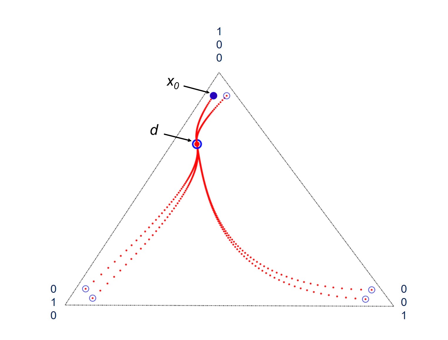
(b)  
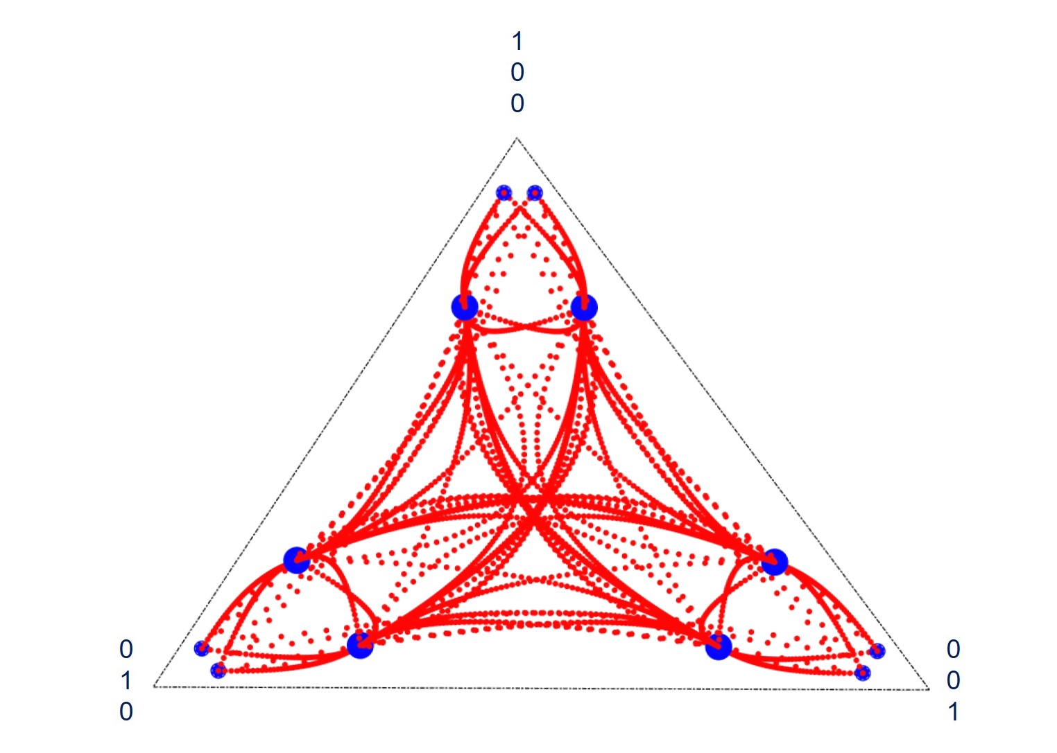
(c) 

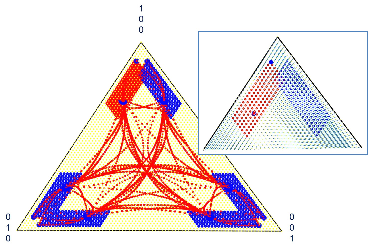
Figure 1: (a) evolutions of initial state $x_{0}=(0.9,0.07,0.03)^{\top}$ and its permutations $\pi(x_{0})$ under $\mathbf{\Gamma}_{d}$ with $V_{1},V_{2}$ of (9) and $\theta=\tfrac{\pi}{6}$ of (11) drive into fixed point $d$.
(b) also includes all permutations of trajectories starting with permutations of $d$, i.e. $x_{0}=\pi(d)$.
(c) the red region shows the states $d$-majorised by $x_{0}$, the blue regions are their permutations; the convex hull over red and blue regions embraces all trajectories and the entire reachable set $\mathfrak{reach}_{\Lambda_{d}}(x_{0})$; the inset gives the vector field to the dynamics $\Lambda_{d}$.

Moreover define the set of vectors in the simplex $\Delta^{n-1}$ that are $d$-majorised by the initial state $x_{0}$ as

$$\Delta^{n-1}_{d}(x_{0}):=\{z\in\Delta^{n-1}\,|\,z\prec_{d}x_{0}\}\,,$$ (14)

while those conventionally majorised by $x_{0}$ shall be denoted as $\Delta^{n-1}_{e}(x_{0})$. For the toy-model dynamics one gets:

• $e^{-tB_{0}}x_{0}\in\Delta^{n-1}_{d}(x_{0})$ for all $t\geq 0$;

• $\Delta^{n-1}_{d}(x_{0})$ is a convex subset within the simplex $\Delta^{n-1}$,

which means the dissipative time evolution of any $x_{0}$ remains within the convex set of states $d$-majorised by $x_{0}$.

Beyond pure dissipative evolution the toy model also allows for permutations $\pi$, so one naturally obtains

$$\mathfrak{reach}_{\Lambda_{d}}(x_{0})=\mathfrak{reach}_{\Lambda_{d}}(\pi(x_{0}))\quad\forall\pi\in\mathcal{S}_{n}\,.$$ (15)

Clearly, the simplex region $\Delta^{n-1}_{d}(x_{0})$ intertwines overall permutations $\pi$ (in the symmetric group $\mathcal{S}_{n}$) in the sense

$$\pi\,\Delta^{n-1}_{d}(x_{0})=\Delta^{n-1}_{\pi(d)}(\pi(x_{0}))\,.$$ (16)

For the maximally mixed state ($d\simeq e$) this boils down to permutation invariance under conventional majorisation

$$\pi\,\Delta^{n-1}_{e}(x_{0})=\Delta^{n-1}_{e}(\pi(x_{0}))=\Delta^{n-1}_{e}(x_{0})\,.$$ (17)

Eq. (16) entails as a first new result:

Theorem 4 (generalising Thm. 3)

Assuming A those initial states $\tilde{x}_{0}$ conventionally majorised by $d$ (i.e. $\tilde{x}_{0}\in\Delta^{n-1}_{e}(d)$) remain within $\Delta^{n-1}_{e}(d)$ under the dynamics of the toy model $\Lambda_{d}$. In other words $\mathfrak{reach}_{\Lambda_{d}}(\tilde{x}_{0})\subseteq\Delta^{n-1}_{e}(d).$

In the next step, writing $x_{0}^{\downarrow}$ for ordering the entries of $x_{0}$ in descending magnitude (so that $x_{0}^{\downarrow}$ and $d$—with $d$ being the thermal state hence sorted by descending entries—are in the same Weyl chamber), one arrives at:

Theorem 5

Under assumption A the reachable set of the dynamics $\Lambda_{d}$ is included in the set of all states conventionally majorised by $\Delta^{n-1}_{d}(x_{0}^{\downarrow})$ in the formal sense

$$\mathfrak{reach}_{\Lambda_{d}}(x_{0})\subseteq\Delta^{n-1}_{e}\big{(}\Delta^{n-1}_{d}(x_{0}^{\downarrow})\big{)}\,.$$ (18)

The proof uses two facts: (i) There exists a (unique) extreme point $z$ of the $d$-majorisation polytope $\Delta^{n-1}_{d}(x_{0}^{\downarrow})$ which conventionally majorises all points in $\Delta^{n-1}_{d}(x_{0}^{\downarrow})$, i.e. $\Delta^{n-1}_{d}(x_{0}^{\downarrow})\subset\Delta^{n-1}_{e}(z)$. (ii) The vector field driving the dynamics of $\Lambda_{d}$ points inside the conventional majorisation polytope $\Delta^{n-1}_{e}(z)$ at each of its $n\/!$ extreme points $\pi(z)$ with $\pi\in\mathcal{S}_{n}$ (cf. Fig. 1(c)). Once knowing how to construct $z$ (see Part-II and [vom Ende and Dirr (2019)] for more detail), the results may be summarised and simplified from $d$-majorisation to conventional majorisation via the extremal state $z$:

Theorem 6

Invoke assumption A. Then for the toy model $\Lambda_{d}$ with Gibbs state $d$ the reachable set is included in the following convex hull

$$\mathfrak{reach}_{\Lambda_{d}}(x_{0})\subseteq\operatorname{conv}\big{\{}\pi(z)\,|\,\pi\in\mathcal{S}_{n}\big{\}}=\Delta^{n-1}_{e}(z)\,.$$ (19)

Fig. 1 illustrates these findings in three-level systems again assuming equidistant separation of energy eigenvalues for the underlying drift term $H_{0}$.

Conclusion and Outlook — For any initial state $x_{0}$, the time evolutions of probability vectors $x(t)$ following the underlying toy model $\Lambda_{d}$ (thermal relaxation interdispersed with level-permutation) remain within the convex hull of extreme points resulting from the set of all states $d$-majorised by the initial state $x_{0}$. Yet, upon moving from the toy model to the full quantum dynamics of thermal relaxation interdispersed with unitary coherent evolution, the scenario gets more involved as the operator-lift to $D$-majorisation does not provide such a simple inclusion.

Fruitful discussion with David Reeb on unital systems at a very early phase of the project is gratefully acknowledged.

References

- Alur et al. (1996) Alur, R., Henzinger, T.A., and Sontag, E.D. (1996). Hybrid Systems III: Verification and Control. Lecture Notes in Computer Science, Vol. 1066. Springer, New York.
- Ando (1989) Ando, T. (1989). Majorization, Doubly Stochastic Matrices, and Comparison of Eigenvalues. Lin. Alg. Appl., 118, 163–248.
- Bergholm et al. (2016) Bergholm, V., Wilhelm, F., and Schulte-Herbrüggen, T. (2016). Arbitrary -Qubit State Transfer Implemented by Coherent Control and Simplest Switchable Local Noise. https://arxiv.org/abs/1605.06473v2.
- Brandão et al. (2015) Brandão, F., Horodecki, M., Ng, N., Oppenheim, J., and Wehner, S. (2015). The Second Laws of Quantum Thermodynamics. Proc. Natl. Acad. Sci. USA, 112, 3275–3279.
- Brockett (1972) Brockett, R.W. (1972). System Theory on Group Manifolds and Coset Spaces. SIAM J. Control, 10, 265–284.
- Chen et al. (2014) Chen, Y., Neill, C., Roushan, P., Leung, N., Fang, M., Barends, R., Kelly, J., Campbell, B., Chen, Z., Chiaro, B., Dunsworth, A., Jeffrey, E., Megrant, A., Mutus, J.Y., O’Malley, P.J.J., Quintana, C.M., Sank, D., Vainsencher, A., Wenner, J., White, T.C., Geller, M.R., Cleland, A.N., and Martinis, J.M. (2014). Qubit Architecture with High Coherence and Fast Tunable Coupling. Phys. Rev. Lett, 113, 220502.
- Dirr et al. (2009) Dirr, G., Helmke, U., Kurniawan, I., and Schulte-Herbrüggen, T. (2009). Lie-Semigroup Structures for Reachability and Control of Open Quantum Systems: Kossakowski-Lindblad Generators form Lie Wedge to Markovian Channels. Rep. Math. Phys., 64, 93–121.
- Dirr et al. (2019) Dirr, G., vom Ende, F., and Schulte-Herbrüggen, T. (2019). Reachable Sets from Toy Models to Controlled Markovian Quantum Systems. Proc. IEEE Conf. Decision Control (IEEE-CDC), 58, 2322. https://arxiv.org/abs/1905.01224.
- Elliott (2009) Elliott, D. (2009). Bilinear Control Systems: Matrices in Action. Springer, London.
- Gorini et al. (1976) Gorini, V., Kossakowski, A., and Sudarshan, E. (1976). Completely Positive Dynamical Semigroups of -Level Systems. J. Math. Phys., 17, 821–825.
- Horn and Johnson (1991) Horn, R.A. and Johnson, C.R. (1991). Topics in Matrix Analysis. Cambridge University Press, Cambridge.
- Horodecki and Oppenheim (2013) Horodecki, M. and Oppenheim, J. (2013). Fundamental Limitations for Quantum and Nanoscale Thermodynamics. Nat. Commun., 4(2059).
- Jurdjevic (1997) Jurdjevic, V. (1997). Geometric Control Theory. Cambridge University Press, Cambridge.
- Jurdjevic and Sussmann (1972) Jurdjevic, V. and Sussmann, H. (1972). Control Systems on Lie Groups. J. Diff. Equat., 12, 313–329.
- Lakshmikantham et al. (1989) Lakshmikantham, V., Bainov, D.D., and Simeonov, P.S. (1989). Theory of Impulsive Differential Equations. Series in Modern Applied Mathematics, Vol. 6. World Scientific, Singapore.
- Lindblad (1976) Lindblad, G. (1976). On the Generators of Quantum Dynamical Semigroups. Commun. Math. Phys., 48, 119–130.
- Marshall et al. (2011) Marshall, A., Olkin, I., and Arnold, B. (2011). Inequalities: Theory of Majorization and Its Applications. Springer, New York, second edition.
- Rooney et al. (2018) Rooney, P., Bloch, A., and Rangan, C. (2018). Steering the Eigenvalues of the Density Operator in Hamiltonian-Controlled Quantum Lindblad Systems. IEEE Trans. Automat. Control, 63, 672–681.
- Veinott (1971) Veinott, A. (1971). Least -Majorized Network Flows with Inventory and Statistical Applications. Manag. Sci., 17, 547–567.
- vom Ende and Dirr (2019) vom Ende, F. and Dirr, G. (2019). The -Majorization Polytope. https://arxiv.org/abs/1911.01061.
- vom Ende et al. (2019) vom Ende, F. , Dirr, G. , Keyl, M. and Schulte-Herbrüggen, T. (2019). Reachability in Infinite-Dimensional Unital Open Quantum Systems with Switchable GKS–Lindblad Generators. Open Sys. Information Dyn., 26, 1950014.
- Wong et al. (2019) Wong, C., Wilen, C., McDermott, R., and Vavilov, M. (2019). A Tunable Quantum Dissipator for Active Resonator Reset in Circuit QED. Quant. Sci. Technol., 4, 025001.
- Yuan (2010) Yuan, H. (2010). Characterization of Majorization Monotone Quantum Dynamics. IEEE. Trans. Autom. Contr., 55, 955–959.