Bayesian Posterior Interval Calibration to Improve the Interpretability of Observational Studies

Abstract

[Abstract]Observational healthcare data offer the potential to estimate causal effects of medical products on a large scale. However, the confidence intervals and p-values produced by observational studies only account for random error and fail to account for systematic error. As a consequence, operating characteristics such as confidence interval coverage and Type I error rates often deviate sharply from their nominal values and render interpretation impossible. While there is longstanding awareness of systematic error in observational studies, analytic approaches to empirically account for systematic error are relatively new. Several authors have proposed approaches using negative controls (also known as "falsification hypotheses") and positive controls. The basic idea is to adjust confidence intervals and p-values in light of the bias (if any) detected in the analyses of the negative and positive control. In this work, we propose a Bayesian statistical procedure for posterior interval calibration that uses negative and positive controls. We show that the posterior interval calibration procedure restores nominal characteristics, such as 95% coverage of the true effect size by the 95% posterior interval.

1 Introduction

Observational healthcare data offer the potential to estimate causal effects of healthcare interventions at scale. However, because of concerns about bias and the appropriate interpretation of the statistical artifacts produced by observational studies, healthcare researchers, practitioners, and regulators have struggled to incorporate observational studies into routine healthcare decision making. Observational studies must consider two sources of error, random and systematic. Random error derives from sampling variability whereas systematic error derives from confounding, measurement error, model mis-specification, and related concerns. Standard statistical methods generally focus exquisitely narrowly on random error and assume there is no systematic error. Ironically, random error generally converges to zero as sample size become larger, precisely the circumstance we now enjoy with large-scale electronic health records. Systematic error, by contrast, persists independently from sample size and thus increases in relative importance. Negative controls, i.e., exposure-outcome pairs where one believes no causal effect exists, have been proposed as a tool to better explain systematic error. ^{1, 2, 3, 4, 5} Executing a study on negative controls and determining whether the results indeed show no effect, that is using them as “falsification hypotheses”, can help detect bias inherent to the study design or data. In order to account for these biases, ⁶ and ⁷ go one step further and incorporate the effect of error observed for negative controls into the estimates from observational studies, in effect calibrating the confidence intervals and p-values. Their methods can also account for positive controls, exposure-outcome pairs where the (non-null) causal effect is known at least approximately.

In this paper, we derive and analyze a Bayesian hierarchical analog to frequentist approaches described in ⁶ and ⁷. We provide a large-scale evaluation in two different clinical contexts, depression and hypertension. The Bayesian approach clarifies the assumptions underlying calibration and facilitates future extensions such as calibrated meta-analysis and calibrated model averaging.

2 Methods

2.1 Basics

We define a cohort $c,c=1,\ldots,C$ as a group of subjects that satisfy one or more criteria for a duration of time. For example, a cohort could comprise individuals newly diagnosed with hypertension, with one year’s observation prior to cohort entry, prescribed a beta blocker at cohort entry, and followed thereafter for two years. A subject can belong to multiple cohorts at the same time, and belong to the same cohort multiple times. For example, a subject could drop in and out of a hypertension cohort according to whether they are taking or not taking a particular drug. We refer to each period of time a subject is in a cohort as an “entry.” We denote by $N_{c}$ the number of entries in cohort $c$ and by $d_{ci}$ the duration (in days) for entry $i$ in cohort $c$. Finally, $N_{c}(t)$ denotes the number of entries in cohort $c$ that span day $t$.

We use cohorts to study associations between interventions and “outcomes.” An outcome (e.g., stroke) occurs at a discrete moment in time and may or may not have a duration. We denote by $y_{ci}$ the number of outcome events observed for entry $i$ in cohort $c$ and by $y_{ci}(t)$ the number of outcome events observed for entry $i$ in cohort $c$ on day $t$.

An “exposure cohort” is a cohort where all entries are exposed to a particular treatment $x,x=1,\ldots,X$. As such, $y_{ci}(x=j)$ denotes the number of outcome events for subject $i$ in exposure cohort $c$ associated with treatment $x=j$. We can also consider a counterfactual cohort, identical in every way, except each subject is unexposed to treatment $j$ at all times while in the cohort. Here. $y_{ci}(x=\lnot j)$ denotes the number of outcome events for patient $i$ in this counterfactual cohort.

We define the causal effect of $x=j$ on $Y$, within some exposure cohort $c$ defined by exposure to $x=j$, as the incidence rate ratio:

$$\mu_{cx}=\frac{\sum_{i}y_{ci}(x=j)/\sum_{i}d_{ci}}{\sum_{i}y_{ci}(x=\lnot j)/\sum_{i}d_{ci}}.$$

Alternatively, we can also formulate the effect as the hazard ratio:

$$h_{cx}(t)=\lim_{\Delta t\to 0}\frac{\sum_{i}y_{ci}(x=j,[t,t+\Delta t])/N_{c}(t)}{\sum_{i}y_{ci}(x=\lnot j,[t,t+\Delta t])/N_{c}(t)}.$$

Note that these quantities estimate the average treatment effect in the treated (ATT) for a cohort.

Finally, $y_{ci}(x=j,t)$ denotes the number of outcome events on day $t$ for subject $i$ in exposure cohort $c$ associated with treatment $x=j$ and $y_{ci}(x=\lnot j,t)$ denotes the corresponding quantity in the counterfactual unexposed cohort.

2.2 Negative and Positive Controls

A "negative control" comprises a target treatment, a comparator treatment, an outcome, and nesting cohort where neither the target treatment nor the comparator treatment are believed to cause the corresponding outcome. Therefore the true effect sizes for the direct causal effect of the target treatment on the outcome, the direct causal effect of the comparator on the outcome, and the comparative effect of the target treatment versus the comparator treatment on the outcome are all 1. For example, consider the first row of Table 1, and let $y$ denote the outcome “acute pancreatitis” and $x=j$ denote the treatment brinzolamide. Because we assume we have a negative control, the relative risk must be 1, and we therefore have

$$y_{ci}(x=j,t)=y_{ci}(x=\lnot j,t),i=1,\ldots,N_{c},t=1,\ldots,d_{ci}.$$

As a consequence, both $\mu_{cx}=1$ and $h_{cx}(t)=1.$

Target	Comparator	Nesting cohort	Outcome	True effect size
Brinzolamide	Levobunolol	Glaucoma	Acute pancreatitis	1.0
Cevimeline	Pilocarpine	Sjogren’s syndrome	Acute pancreatitis	1.0
Diclofenac	Celecoxib	Arthralgia	Acute stress disorder	1.0
Diclofenac	Celecoxib	Arthralgia	Ingrowing nail	1.0

Table 1: Example negative controls.

We generate synthetic "positive controls" from negative controls by adding simulated additional outcomes in the target treatment cohort until a desired incidence rate ratio is achieved. For example, assume that, during treatment with diclofenac, $m$ occurrences of ingrowing nail were observed. None of these were caused by diclofenac since this is one of our negative controls. If we were to add an additional $m$ simulated occurrences during treatment with diclofenac, we would have doubled the observed effect size. Since this was a negative control, and since only the treatment cohort received new ingrowing nails and not the counterfactual cohort, the observed relative risk which was one becomes two.

More specifically, let $\theta$ denote the target effect size. Currently we use $\theta=1.5,\theta=2$ and $\theta=4$ to generate 3 positive controls from every negative control. We increase outcome count $y_{ci}(x=j)$ in the target treatment ($j$) cohort to $y_{ci}^{*}(x=j)$ to approximate the desired $\theta$. To avoid issues due to low sample size, we generate positive controls only when $y_{ci}\geq 25.$

The steps in the “injection” process are as follows:

1. Within the target treatment cohort $c$, we fit an L1-regularized Poisson regression model where the outcome $y_{ci}(x=j)$ represents the subject-level dependent variable and $Z_{ci}$ represents the independent variables. The independent variables include demographics, as well as all recorded diagnoses, drug exposures, measurements, and medical procedures all measured prior to cohort entry (“baseline covariates”). We use 10-fold cross-validation to select the regularization hyperparameter. Let $\hat{\lambda}_{ci}=E(y_{ci}|Z_{ci})$ denote the predicted Poisson event rate for entry $i$ in treatment cohort $c$.

2. For every entry in the target treatment cohort, sample $n$ from a Poisson distribution with parameter $(\theta-1)\hat{\lambda}_{ci}$ and set $y_{ci}^{*}(x=j)=y_{ci}(x=j)+n.$

3. Repeat step 2 until $\lvert\frac{\sum_{i}y_{ci}^{*}(x=j)/\sum_{i}d_{ci}}{\sum_{i}y_{ci}(x=j)/\sum_{i}d_{ci}}-\theta\rvert\leq\epsilon,$ where $\epsilon$ is currently set to 0.01.

Assuming the synthetic outcomes have the same measurement error (same positive predictive value and sensitivity) as the observed outcomes, this process creates data that mimic a true marginal effect size of $\theta$. Because we sample new outcomes from a large-scale predictive model, we also mimic the conditional effect (conditional on $Z$). We note that the altered data can capture effects due to measured confounding but not unmeasured confounding.

2.3 Frequentist Calibration

In prior work, we described a method for empirically calibrating p-values. ⁸ Briefly, when evaluating a particular analytical method, the calibration procedure applies the method not only to the target-comparator-outcome of interest but also to all the negative controls. This generates draws from an “empirical” null distribution. By contrast with the theoretical null distribution (typically a Gaussian centered on 1), the empirical null distribution does not assume that the estimated effect size provides an unbiased estimate of the true effect. Instead the location and dispersion of the empirical null distribution reflects both random error and systematic error. “Calibrated” or “empirical” p-values use the empirical null distribution in place of the theoretical null distribution when computing p-values.

More formally, let $\hat{\theta}_{i}$ denote the estimated log effect estimate (relative risk, odds or incidence rate ratio) from the $i$th negative control, and let $\hat{\tau}_{i}$ denote the corresponding estimated standard error, $i=1,\ldots,n$. Let $\theta_{i}$ denote the true log effect size (assumed 0 for negative controls), and let $\beta_{i}$ denote the true (but unknown) bias associated with pair $i$, that is, the difference between the log of the true effect size and the log of the estimate that the study would have returned for control $i$ had it been infinitely large. As in the standard p-value computation, we assume that $\hat{\theta}_{i}$ is normally distributed with mean $\theta_{i}+\beta_{i}$ and variance $\hat{\tau}_{i}^{2}$. Note that in traditional p-value calculations, $\beta_{i}$ is assumed to be equal to zero for all $i$. Instead we assume the $\beta_{i}$’s arise from a normal distribution with mean $\nu$ and variance $\sigma^{2}$. This represents the null (bias) distribution. We estimate $\nu$ and $\sigma^{2}$ via maximum likelihood. In summary, we assume the following:

$$\beta_{i}\sim N(\nu,\sigma^{2})\>{\rm and}\>\hat{\theta}_{i}\sim N(\theta_{i}+\beta_{i},\hat{\tau}_{i}^{2}),$$

where $N(a,b)$ denotes a normal distribution with mean $a$ and variance $b$, and we estimate $\nu$ and $\sigma^{2}$ by maximizing:

$$\prod_{i=1}^{n}\int p(\hat{\theta}_{i}\mid\beta_{i},\theta_{i},\hat{\tau}_{i}^{2})p(\beta_{i}\mid\nu,\sigma^{2})d\beta_{i}$$

yielding maximum likelihood estimates $\hat{\nu}$ and $\hat{\sigma}^{2}$. We compute a calibrated p-value that uses the empirical null distribution. Let $\hat{\theta}_{0}$ denote the log of the effect estimate for the outcome of interest, and let $\hat{\tau}_{0}$ denote the corresponding (observed) estimated standard error. Assuming $\beta_{n+1}$ arises from the same null distribution, we have that:

$$\hat{\theta}_{0}\sim N(\hat{\nu},\hat{\sigma}^{2}+\hat{\tau}_{0}^{2}),$$

and the p-value calculation follows naturally.

A later paper⁶ used positive controls to extend the concept of calibrated p-values to calibrated confidence intervals. These intervals reflect actual accuracy on negative and positive controls and, like calibrated p-values, capture both random and systematic error. More specifically, they assumed that $\beta_{i}$, the bias associated with control $i$, again comes from a Gaussian distribution, but this time using a mean and standard deviation that are linearly related to $\theta_{i}$, the true effect size:

$$\beta_{i}\sim N(\nu(\theta_{i}),\sigma^{2}(\theta_{i}))$$

where:

$$\nu(\theta_{i})=a+b\theta_{i}\;{\rm and}\;\sigma^{2}(\theta_{i})=c+d\times\mid\theta_{i}\mid.$$

We estimate $a,b,c$ and $d$ by maximizing the marginalized likelihood in which we integrate out the unobserved $\beta_{i}$:

$$\prod_{i=1}^{n}\int p(\hat{\theta}_{i}\mid\beta_{i},\theta_{i},\hat{\tau}^{2}_{i})p(\beta_{i}\mid a,b,c,d,\theta_{i})d\beta_{i}$$

yielding $(\hat{a},\hat{b},\hat{c},\hat{d})$. We compute a calibrated CI that uses the systematic error model. Let $\hat{\theta}_{0}$ again denote the log of the effect estimate for the outcome of interest, and let $\hat{\tau}_{n+1}$ denote the corresponding (observed) estimated standard error. Then:

$$\hat{\theta}_{0}\sim N(\theta_{0}+\hat{a}+\hat{b}\times\theta_{0},\hat{c}+\hat{d}\times\mid\theta_{0}\mid+\hat{\tau}^{2}_{0}),$$

and the calibrated confidence interval follows.

Our prior work has also shown that, unlike standard confidence intervals, calibrated confidence intervals maintain coverage at or close to the desired level, e.g., 95%. Typically, but not necessarily, the calibrated confidence interval is wider than the nominal confidence interval, reflecting the problems unaccounted for in the standard procedure (such as unmeasured confounding, selection bias and measurement error) but accounted for in the calibration.

2.4 Bayesian Calibration

In this work, we use a hierarchical Bayesian approach to perform the calibration. We consider two different models of the bias, a model that is not dependent on the true effect sizes, and a model that is linearly dependent on the true effect sizes.

Again, let $\theta_{0}$ denote the log of the true effect size (relative risk, odds ratio, or hazard ratio) of interest. Let $\theta_{i}$ denote the log of the true effect size for the available negative and positive controls, where $i=1,\ldots,m$. We use $\hat{\theta}_{i}$ to denote the log of the estimated effect sizes, where $i=0,\ldots,m$, and $\hat{\tau_{i}}$ to denote the corresponding estimated standard error. In what follows, we will again assume that the $\beta_{i}$’s are normally distributed. In practice, as shown below, this yields good empirical results but future refinements could consider more flexible models.

2.4.1 Constant Model of the True Bias

Let $\hat{\beta}_{i}=\hat{\theta}_{i}-\theta_{i}$ denote the "estimated bias," where $i=0,\ldots,m$.

Then we propose the following hierarchical model:

$$\beta_{i} \sim N(\mu,\sigma^{2}),\;i=0,\ldots,m$$ (1)

$$\hat{\beta}_{i} \sim N(\beta_{i},\hat{\tau}_{i}^{2}),\;i=0,\ldots,m$$ (2)

Note in the above model, it is possible to integrate out the $\beta_{i}$’s since:

$$\hat{\beta}_{i}\sim N(\mu,\sigma^{2}+\hat{\tau}_{i}^{2})$$ (3)

We give $\mu$ and $\sigma^{2}$ relatively noninformative priors, $\mu\sim N(0,50)$ and $1/\sigma^{2}\sim U(0,100)$, where $U$ stands for the uniform distribution. See Figure 1 for a graphical model representation.

Figure 1: Graphical Model for Constant Model of the True Bias.

2.4.2 Linear Model of the True Bias

We compare the results of the constant model described in 2.4.1 of the true bias to the linear model described in ⁶. Following ⁶, we reconstruct the linear model of true bias of using the modified hierarchical model:

$$\beta_{i}\sim N(\mu+c\theta_{i},\sigma^{2}+d\theta_{i}),\;i=0,\ldots,m$$ (4)

where $\mu{\sim}N(0,50)$, $1/{\sigma}^{2}{\sim}U(0,100)$, $c{\sim}N(0,50),$ and $d{\sim}N(0,50)$. See Figure 2 for a graphical model representation.

Figure 2: Graphical Model for Linear Model of the True Bias.

2.4.3 Experimental Design and Computation

We consider two approaches to evaluating Bayesian calibration. For the first approach, we train the Bayesian calibration method on 80% of the treatment-comparator-outcome (TCO) triples using both positive and negative controls, and test the effect size of interest using the remaining TCOs. Since the positive controls are simulated from the negative controls, we take care to test the positive and negative controls that were not used in the same TCO combinations from the training data set. We evaluate both models of bias, the simple model and the linear model, using this training data set.

For the second approach of evaluating Bayesian calibration, and to address concerns about the fidelity of the positive controls with respect to unmeasured confounding and the actual true effect sizes, we train the Bayesian calibration method on 80% of the negative control combinations, and test the positive and negative controls that were not used in the same TCO combinations from the training data set. Due to the nature of the linear model, we can only evaluate the constant bias model using this training data set.

We use Markov chain Monte Carlo, specifically a Gibbs sampler, to estimate the log of the effect sizes for the Bayesian calibration procedure. We specify three parallel chains, 1000 burn-in and adaptive iterations, thinning of one, and 1000 additional samples to take. Initial values for each chain are specified to have a mean of zero and a variance of one. The trace, histogram, empirical cumulative distribution function, and autocorrelation plots reflect adequate convergence.

2.4.4 Description of the Data

We consider two data sets for the analysis, one with treatments for depression and another with treatments for hypertension.

For the depression data set, we used the results described in ⁷. ⁷ reported a large-scale comparative effectiveness study of 17 treatments for depression with respect to 22 outcomes in four large-scale observational databases. Using a new-user propensity-adjusted cohort design, they reported 5,984 estimated effect sizes and corresponding nominal and calibrated 95% confidence intervals. Negative controls were identified for the 17 treatments by selecting outcomes that are well studied, but for which no evidence in the literature suggests a relationship with any of the 17 treatments. A total of 52 negative control outcomes were selected. ⁷ Since real positive controls for observational research are difficult to obtain in practice, ⁷ generated synthetic positive controls by modifying a negative control through injection of additional, simulated occurrences of the outcome. The injected extra outcome occurrences were drawn from a high-dimensional patient-level predictive model. For each negative control that has a relative risk of 1, three positive controls were generated, with relative risks of 1.5, 2, and 4. The four databases included in the study for the depression data set were 1) Truven MarketScan Multi-state Medicaid (MDCD), 2) OptumInsight’s de-identified Clinformatics Datamart (Optum), 3) Truven MarketScan Medicare Supplemental Beneficiaries (MDCR), and 4) Truven MarketScan Commercial Claims and Encounters (CCAE). These databases and the procedure for selecting negative and positive controls are described in detail in ⁷.

Similar procedures were employed for the generation of the hypertension data set. The hypertension treatments consists of six administrative claims databases and three electronic health record databases. The databases are: 1) IBM MarketScan Multi-state Medicaid (MDCD), 2) Optum ClinFormatics (Optum), 3) IBM MarketScan Medicare Supplemental Beneficiaries (MDCR), 4) IBM MarketScan Commercial Claims and Encounters (CCAE), 5) Japan Medical Data Center (JMDC), 6) IMS/Iqvia Disease Analyzer Germany (IMSG), 7) Optum Pan-Therapeutic (Panther), 8) Korea National Health Insurance Service / National Sample Cohort (NHIS NSC), and 9) Columbia University Medical Center (CUMC). These databases and the generation of the negative and synthetic positive controls are described in detail in ⁹.

3 Results

3.1 Depression

3.1.1 Constant Model of the True Bias

We first consider the results for the constant model of the true bias on the depression data set.

Train on Negative and Positive Controls

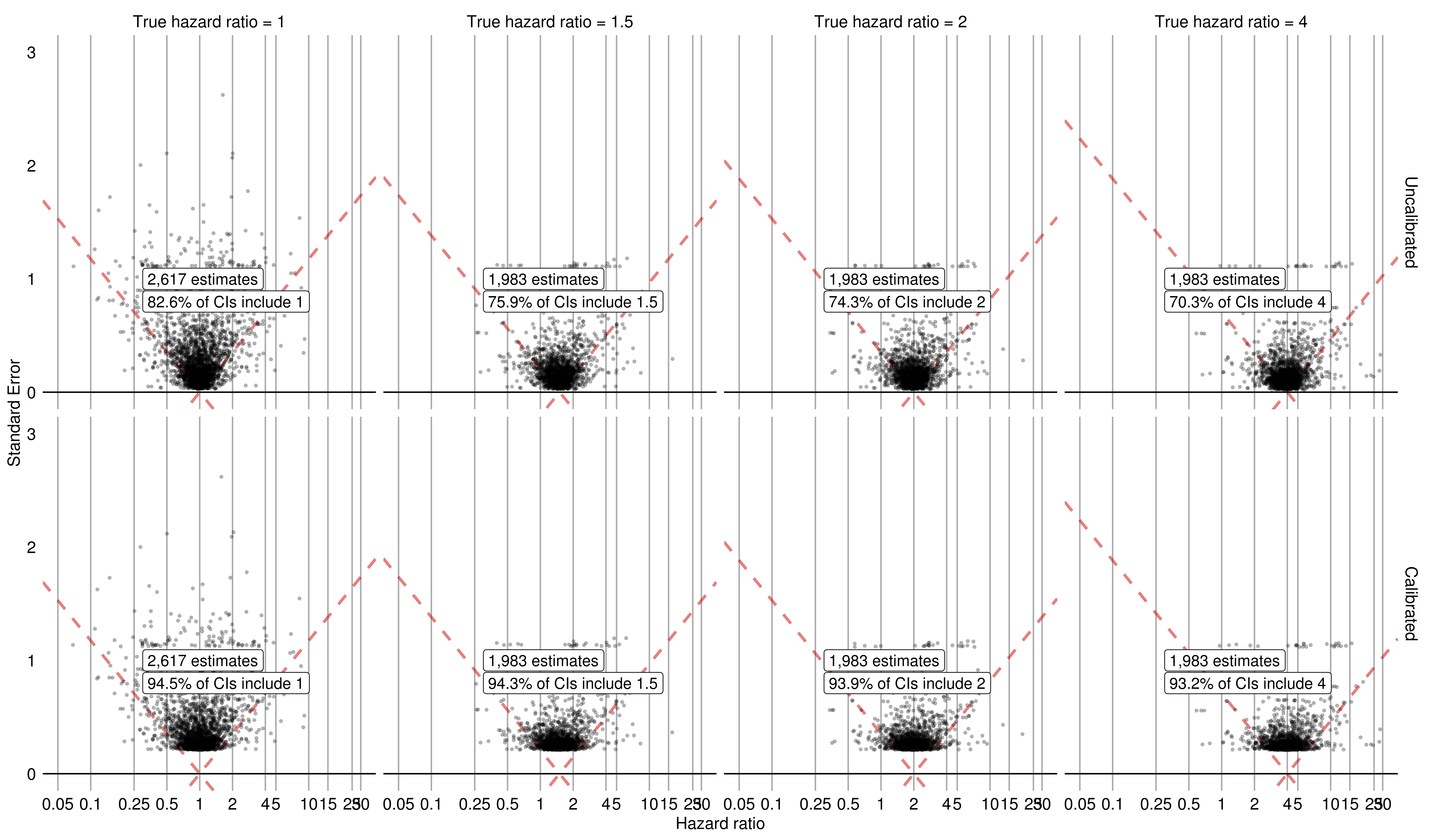
Figure 6: Evaluation of the effect estimation before (top) and after (bottom) calibration using the CCAE database in the depression data set. The constant model of bias was used and training was performed on both negative and positive controls.

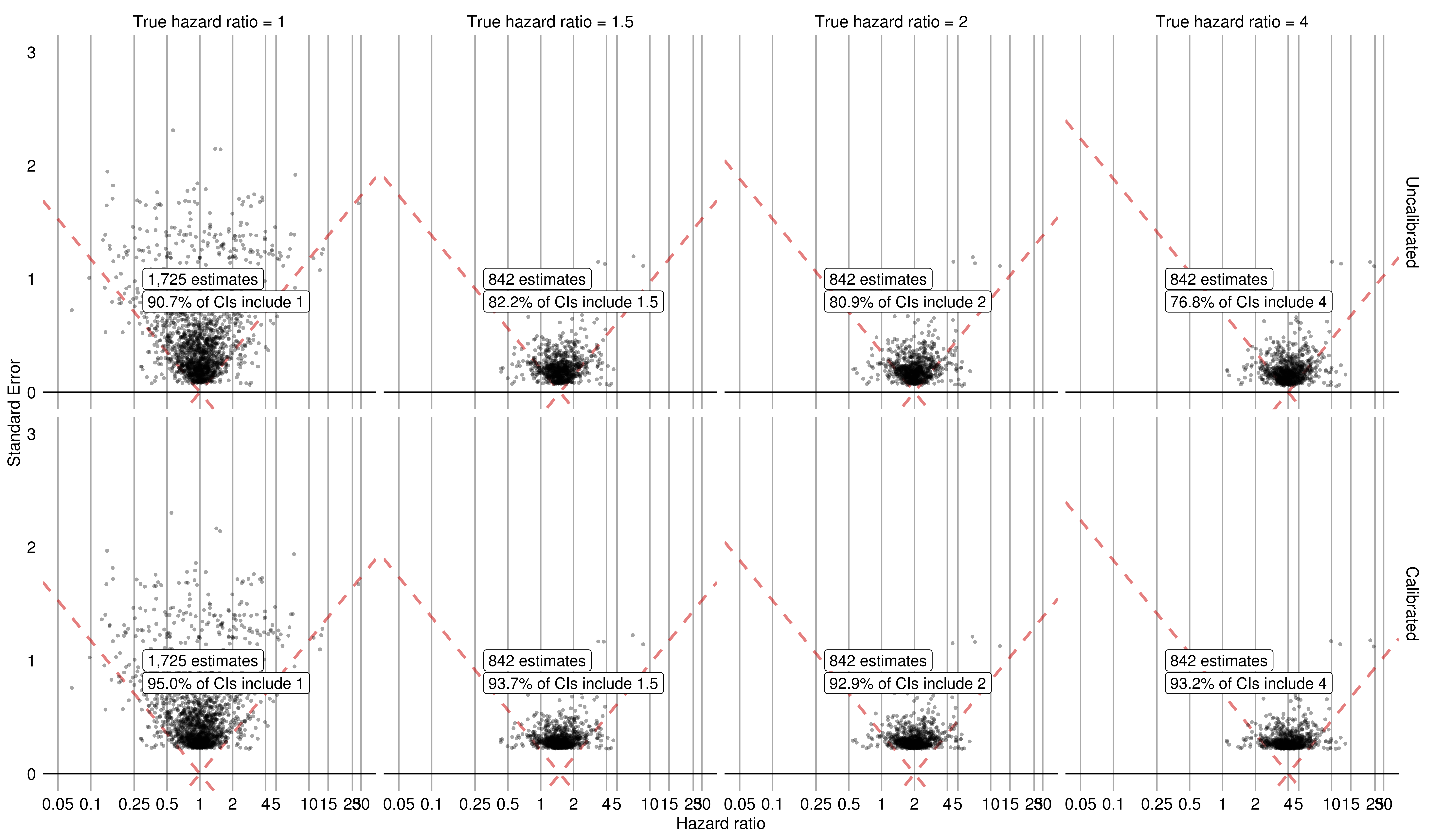
Figure 7: Evaluation of the effect estimation before (top) and after (bottom) calibration using the MDCD database in the depression data set. The constant model of bias was used and training was performed on both negative and positive controls.

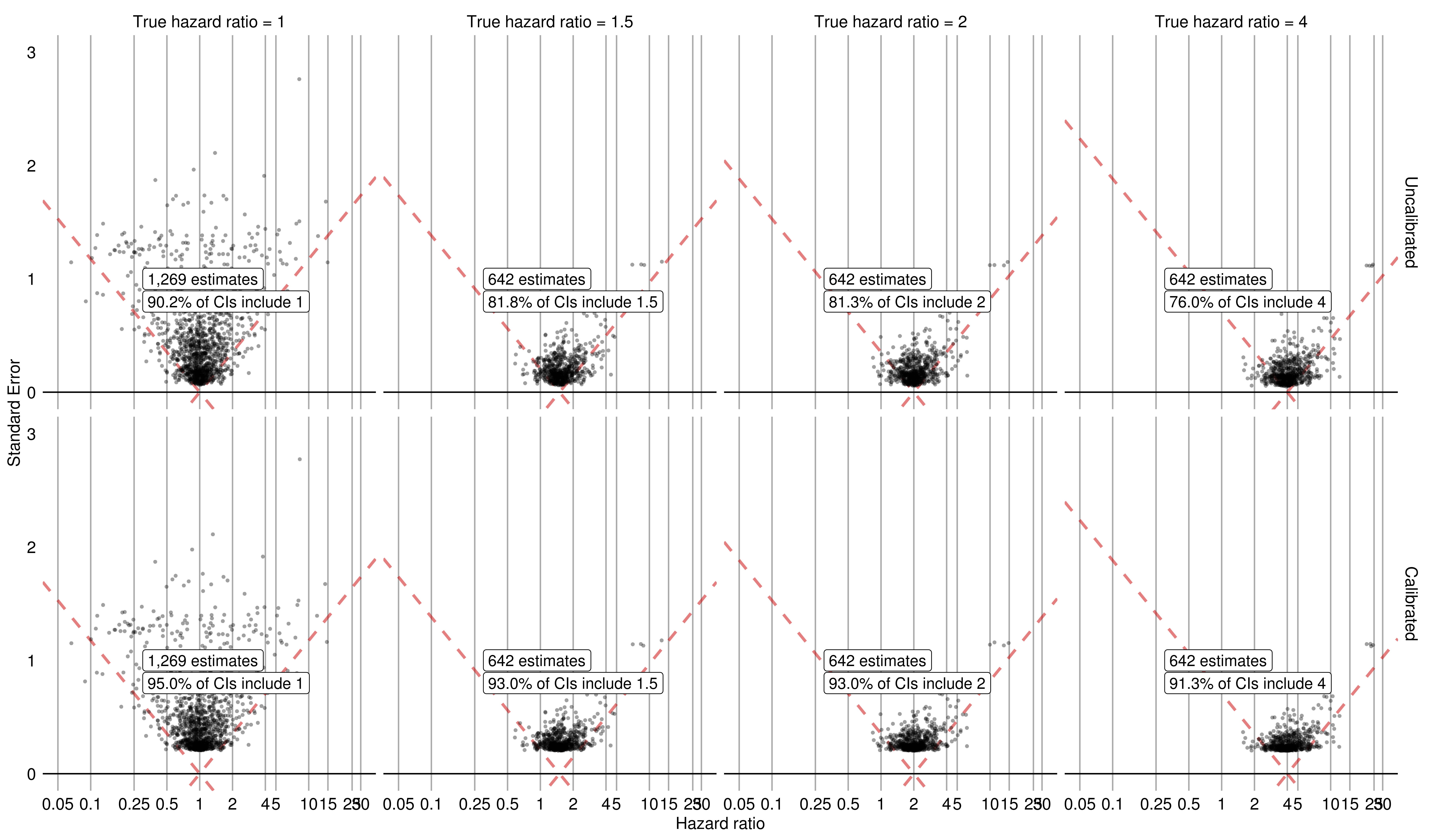
Figure 8: Evaluation of the effect estimation before (top) and after (bottom) calibration using the MDCR database in the depression data set. The constant model of bias was used and training was performed on both negative and positive controls.

We train on both negative and positive controls. We report effect size estimates for all negative and positive controls across the four databases as well as the percentage of posterior intervals containing the true effect size. Figure 3 shows the results using the Optum database and Figures 6, 7, and 8 show the results using the CCAE, MDCD, and MDCR databases, respectively. The number of observations that were tested are reported on the figures. Each dot represents the hazard ratio and corresponding standard error for one of the negative (true hazard ratio = 1) or positive control (true hazard ratio greater than 1) outcomes. Pre-calibration posterior interval coverage departs significantly from 95% especially for the larger positive controls. For all four databases, the calibrated procedure results in posterior intervals that are closer to the nominal 95% coverage than the uncalibrated procedure.

We also report the root mean squared error (RMSE) as a metric to quantify overall coverage across all estimates. We define RMSE as

$$RMSE=\sqrt{\frac{\sum_{t=1}^{T}(\hat{w}-w)^{2}}{T}},$$

where $\hat{w}$ is the number of times that the true effect size is contained in the confidence interval calculated by the calibrated and uncalibrated procedures, divided by the number of observations that were tested, $w=0.95$ to represent the 95% coverage of the true effect size, and $T=4$ for the four hazard ratios (1, 1.5, 2, and 4).

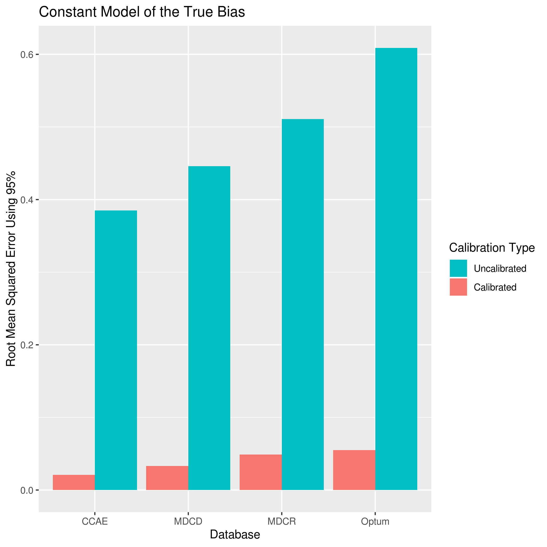
Figure 15: Root mean squared error of all estimated effects before (uncalibrated) and after (calibrated) calibration for each of the databases in the depression data set. The constant model of bias was used and training was performed on both negative and positive controls.

The RMSE for the Optum database using calibration is about 0.05 while without calibration, it is about 0.61. Figure 15 shows the calculated RMSE for each database. Overall, the uncalibrated procedure has higher error than the calibrated procedure. Interestingly, the CCAE database has the lowest error among the two procedures, compared to the Optum database.

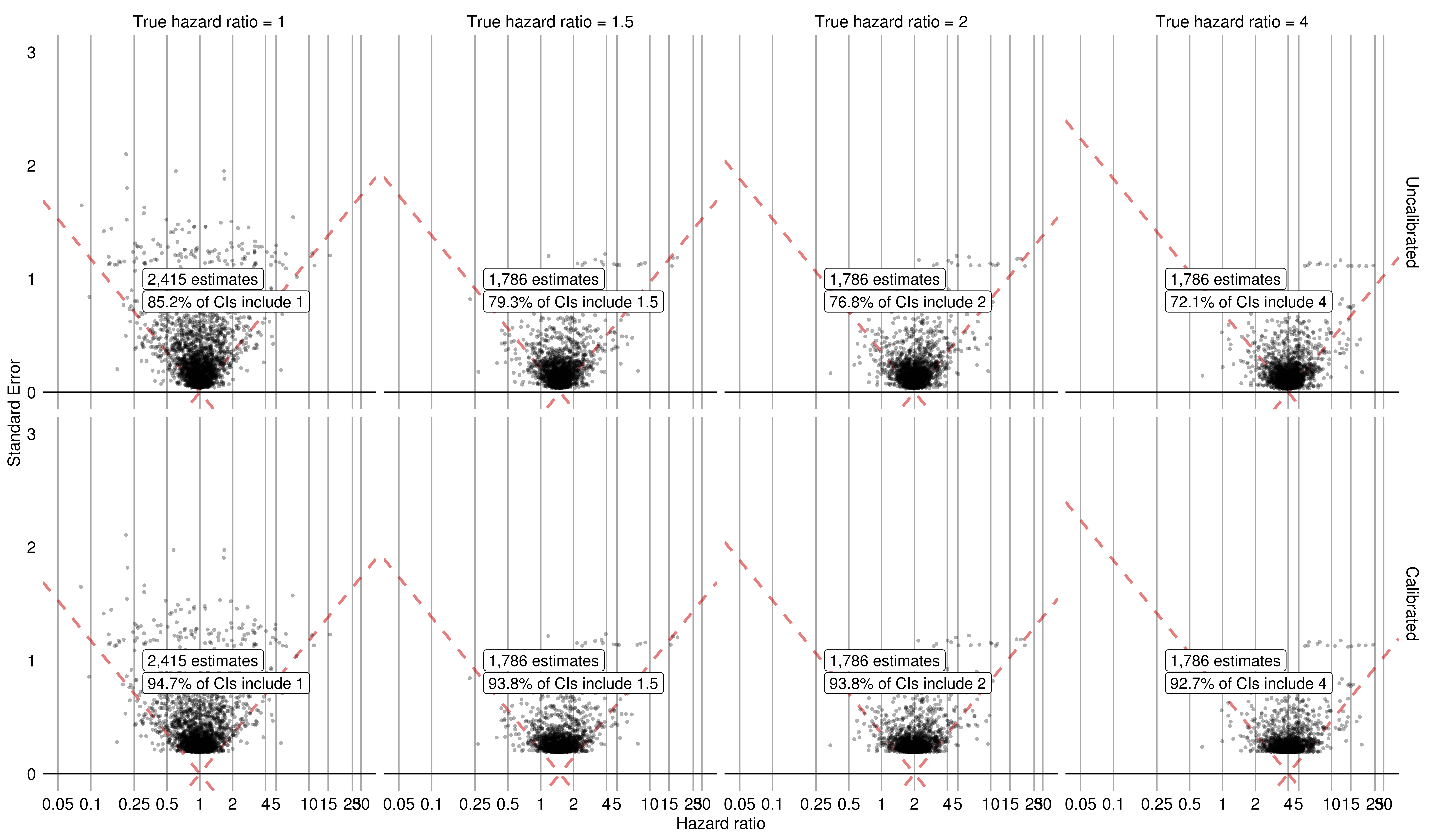
Figure 3: Evaluation of the effect estimation before (top) and after (bottom) calibration using the Optum database in the depression data set. The constant model of bias was used and training was performed on both negative and positive controls.

Train on Only Negative Controls

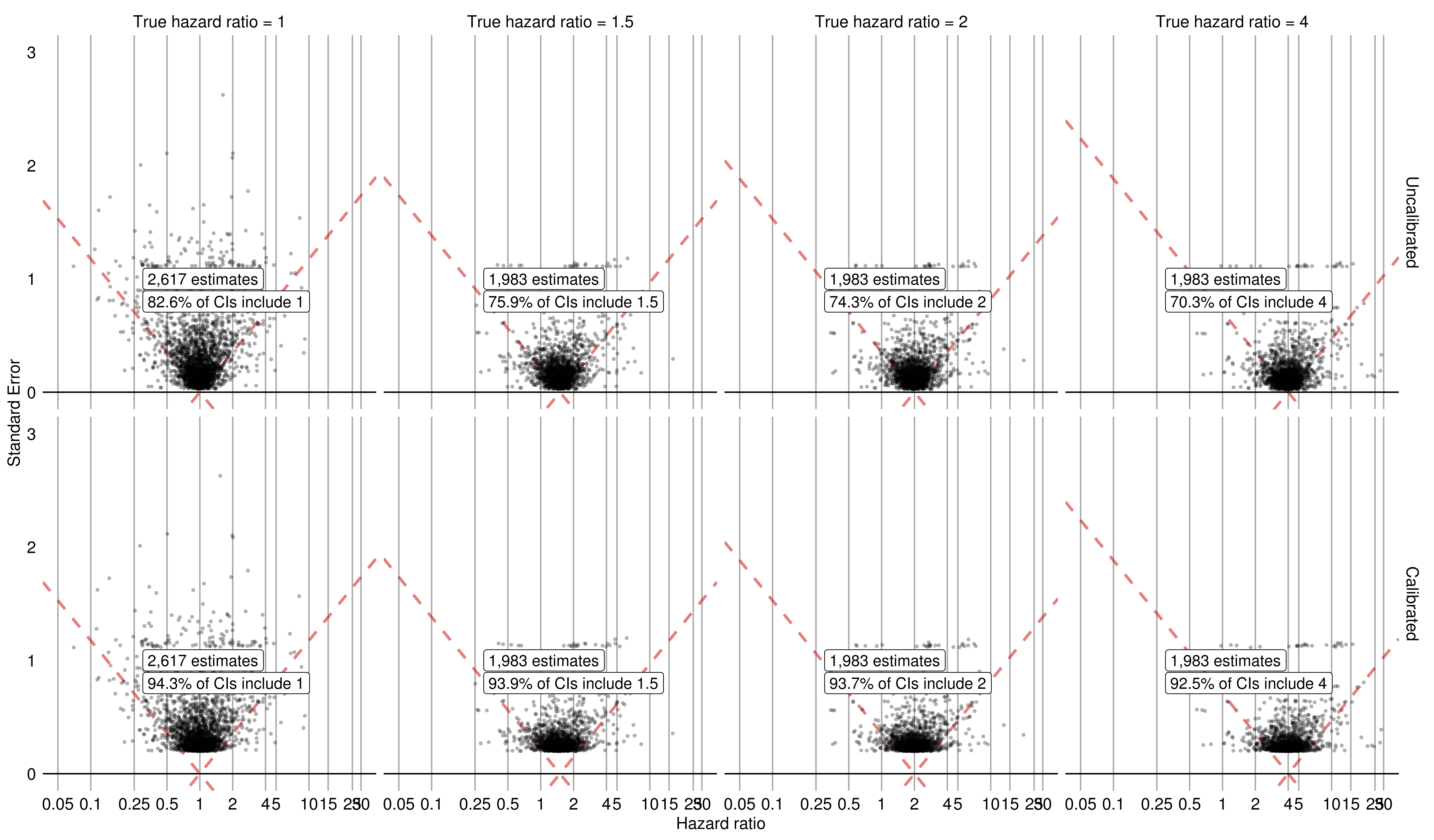
Figure 9: Evaluation of the effect estimation after stratification on the propensity scores before (top) and after (bottom) calibration using the CCAE database in the depression data set. The constant model of bias was used and training was performed on only negative controls.

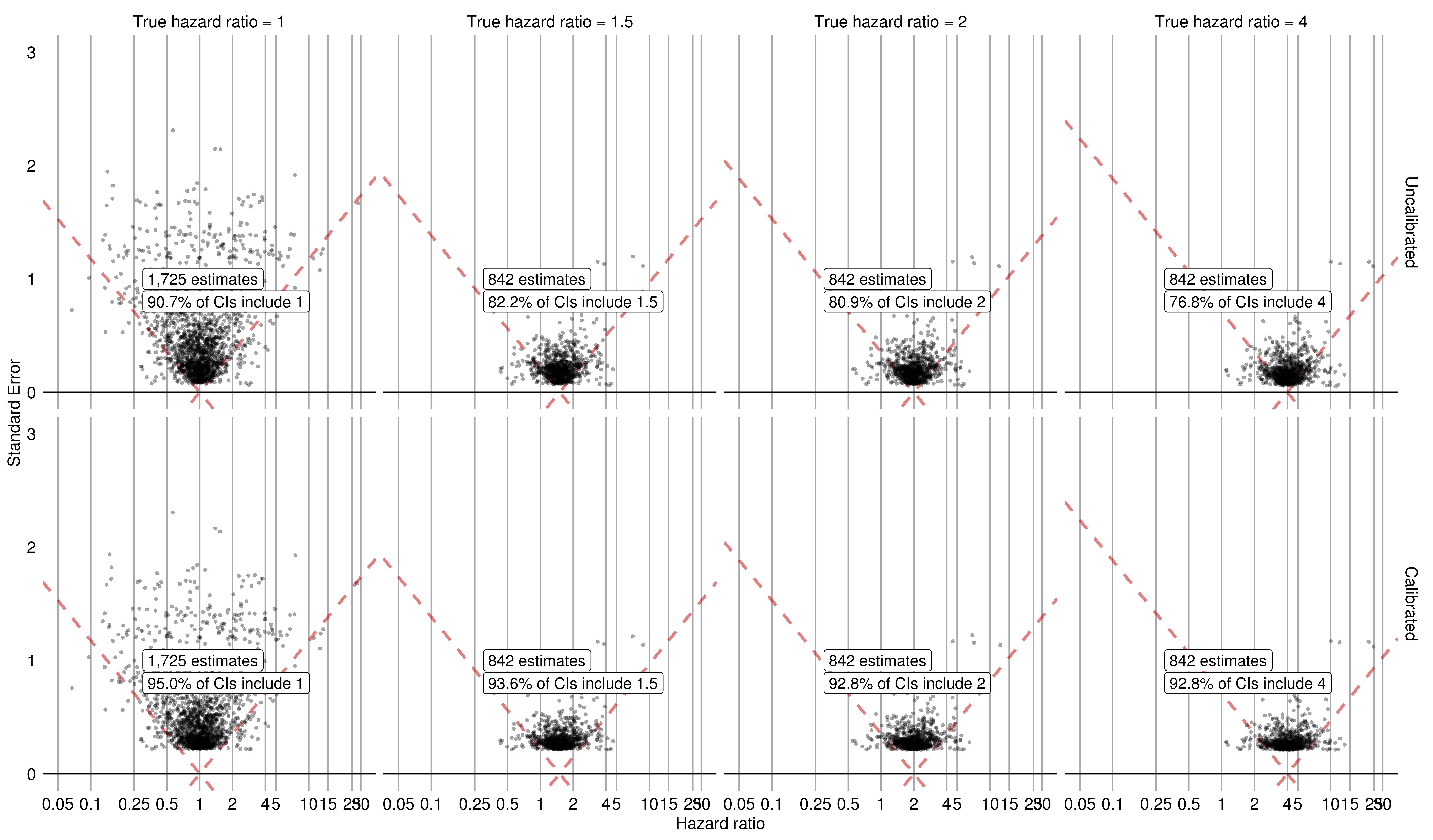
Figure 10: Evaluation of the effect estimation after stratification on the propensity scores before (top) and after (bottom) calibration using the MDCD database in the depression data set. The constant model of bias was used and training was performed on only negative controls.

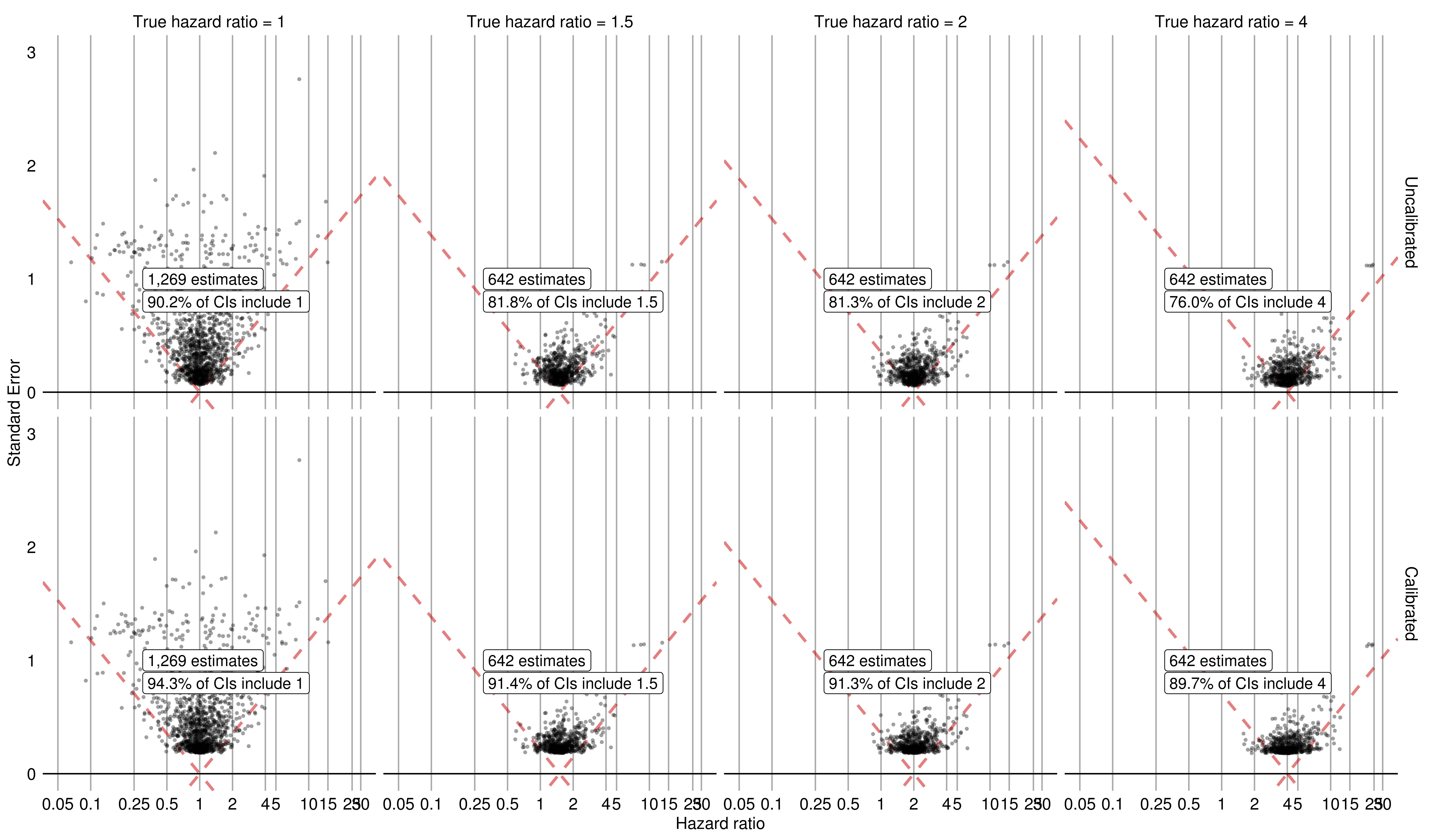
Figure 11: Evaluation of the effect estimation after stratification on the propensity scores before (top) and after (bottom) calibration using the MDCR database in the depression data set. The constant model of bias was used and training was performed on only negative controls.

We also consider the effect of training on negative controls only. Figures 4, 9, 10, and 11 report effect size estimates for all negative and positive controls across the four databases as well as the percentage of posterior intervals containing the true effect size. The number of effect sizes that were tested are reported on the figures. Again, for all four databases, the calibrated procedure results in posterior intervals that are closer to 95% than the uncalibrated procedure. When comparing the effect of training on both negative controls and positive controls to training only on negative controls for the calibrated procedure, overall, there appears to be a slight improvement in posterior interval coverage when training on both negative controls and positive controls. The RMSE for the Optum database using calibration is about 0.08 while without calibration, it is about 0.61. Figure 16 shows the RMSE calculated for each database. Again, the uncalibrated procedure has higher error than the calibrated procedure, when considering all hazard ratios combined.

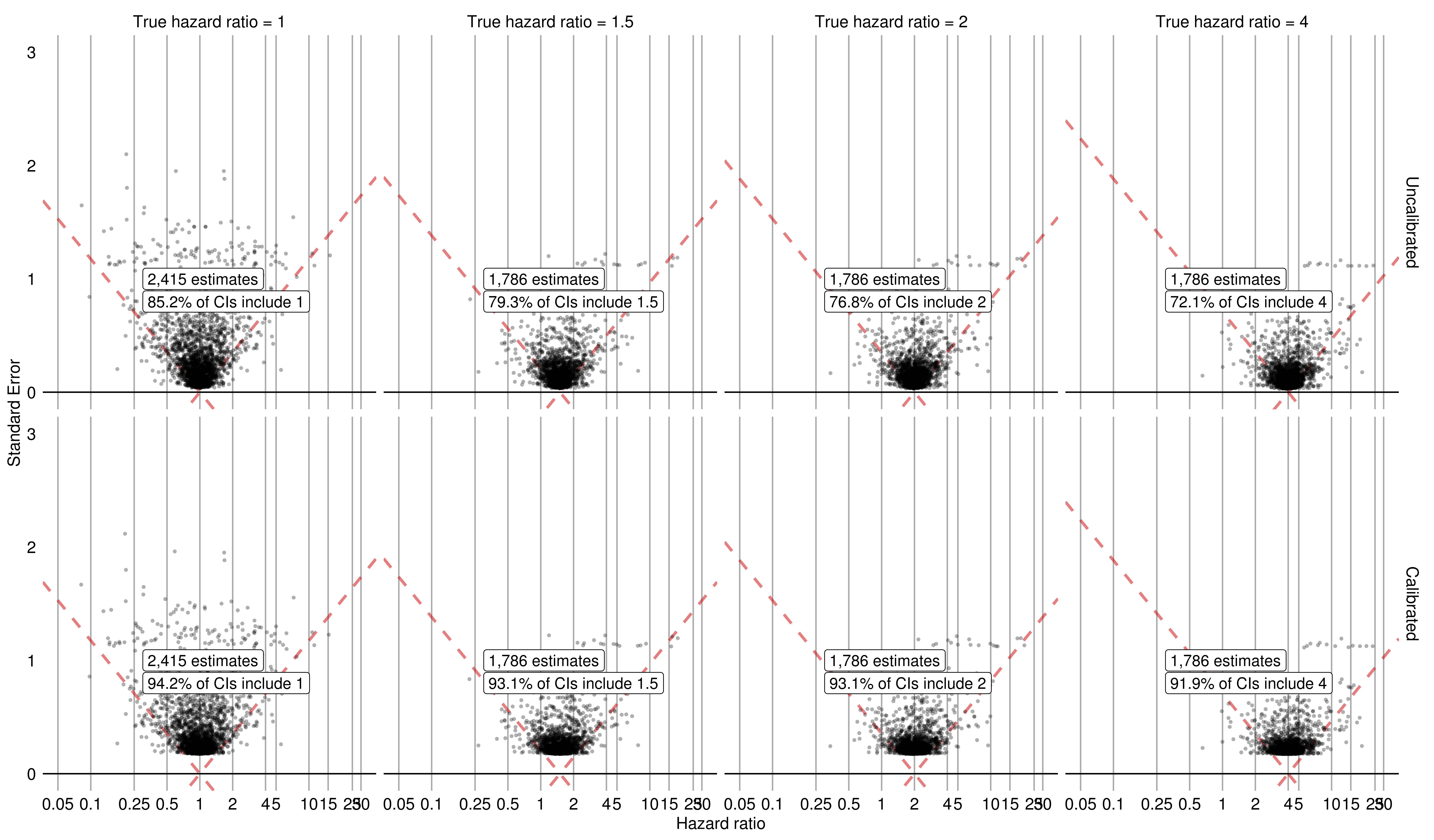
Figure 4: Evaluation of the effect estimation after stratification on the propensity scores before (top) and after (bottom) calibration using the Optum database in the depression data set. The constant model of bias was used and training was performed on only negative controls.

3.1.2 Linear Model of the True Bias

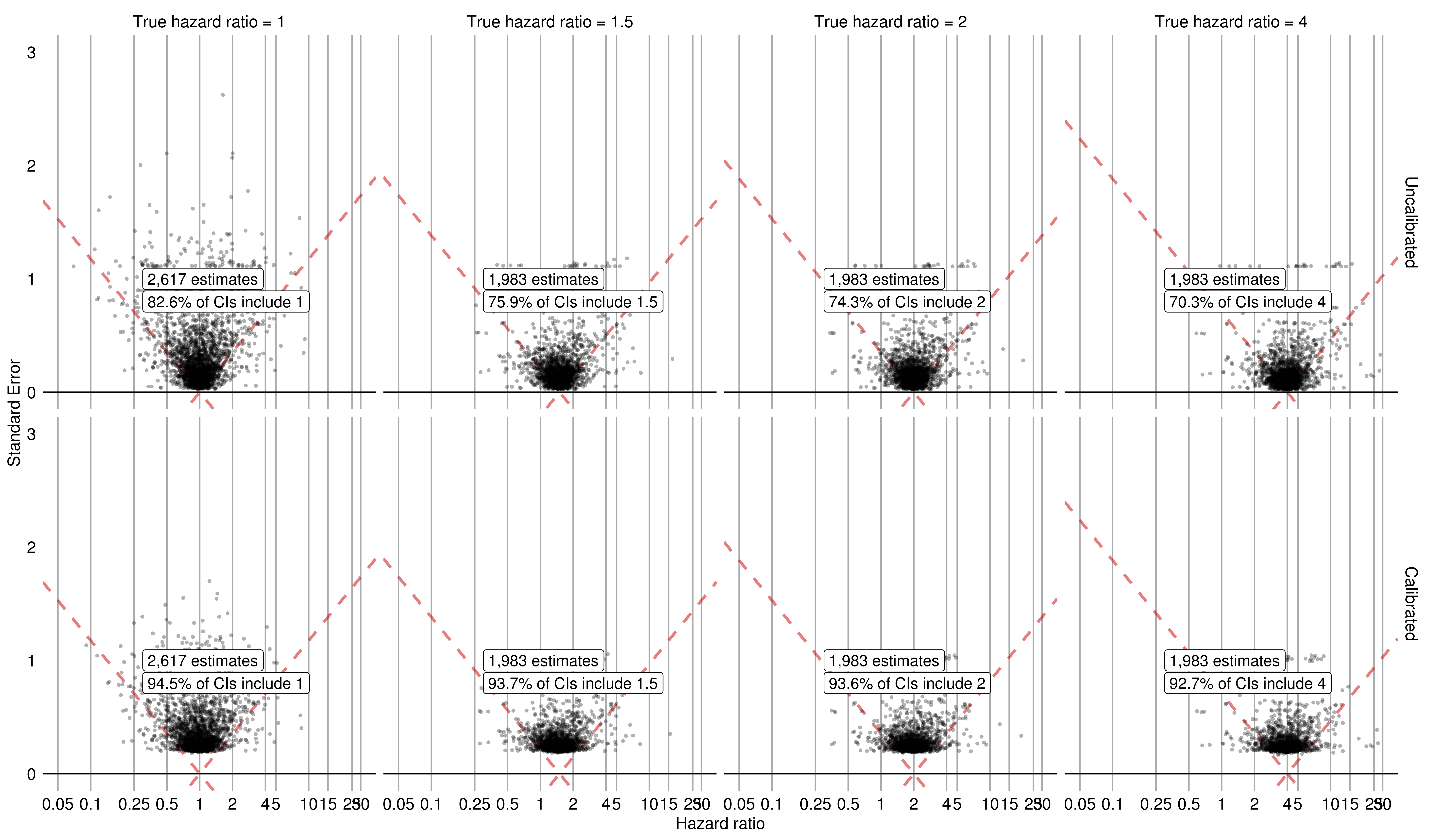
Figure 12: Evaluation of the effect estimation before (top) and after (bottom) calibration using the CCAE database in the depression data set. The linear model of bias was used and training was performed on both negative and positive controls.

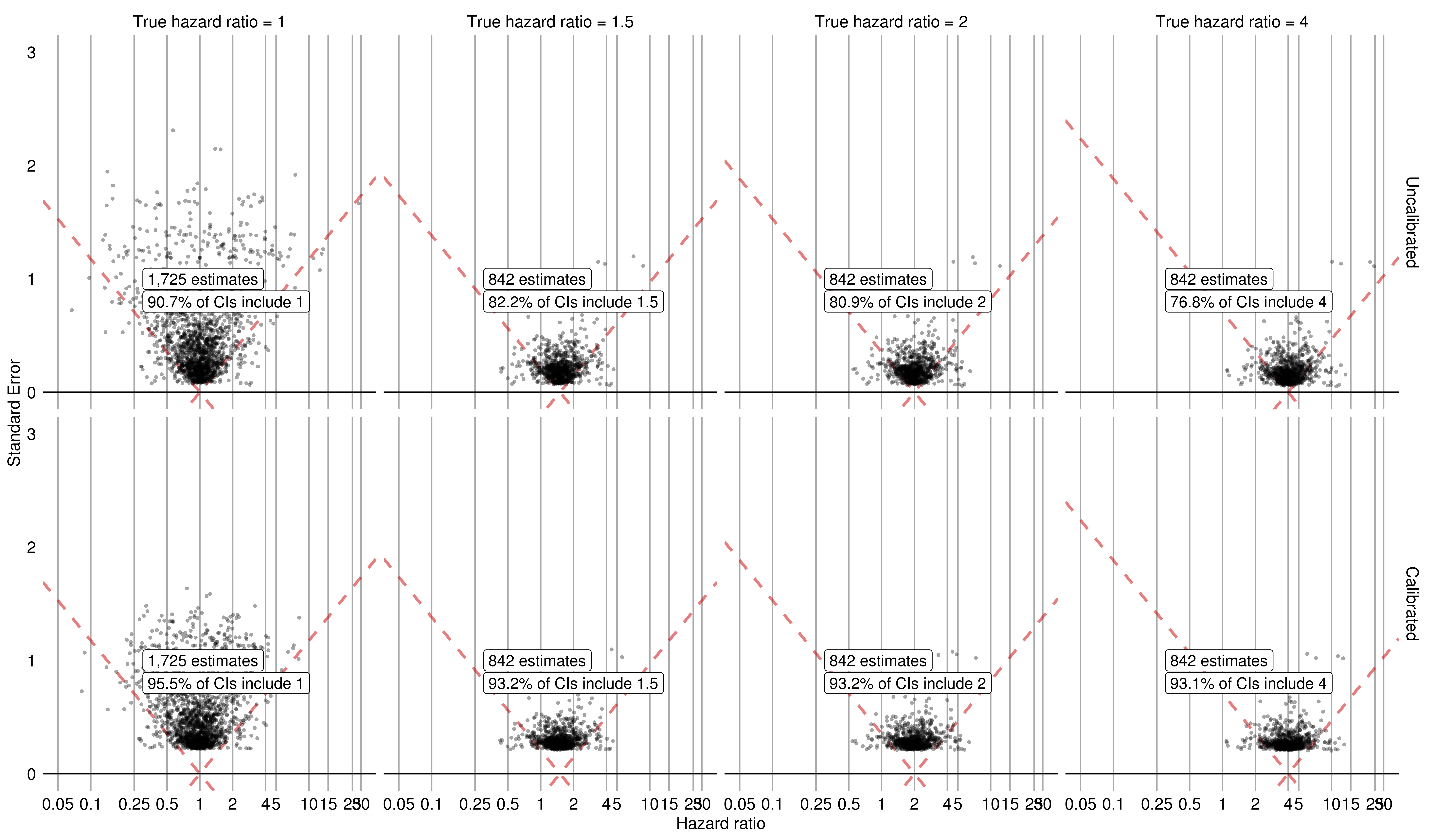
Figure 13: Evaluation of the effect estimation before (top) and after (bottom) calibration using the MDCD database in the depression data set. The linear model of bias was used and training was performed on both negative and positive controls.

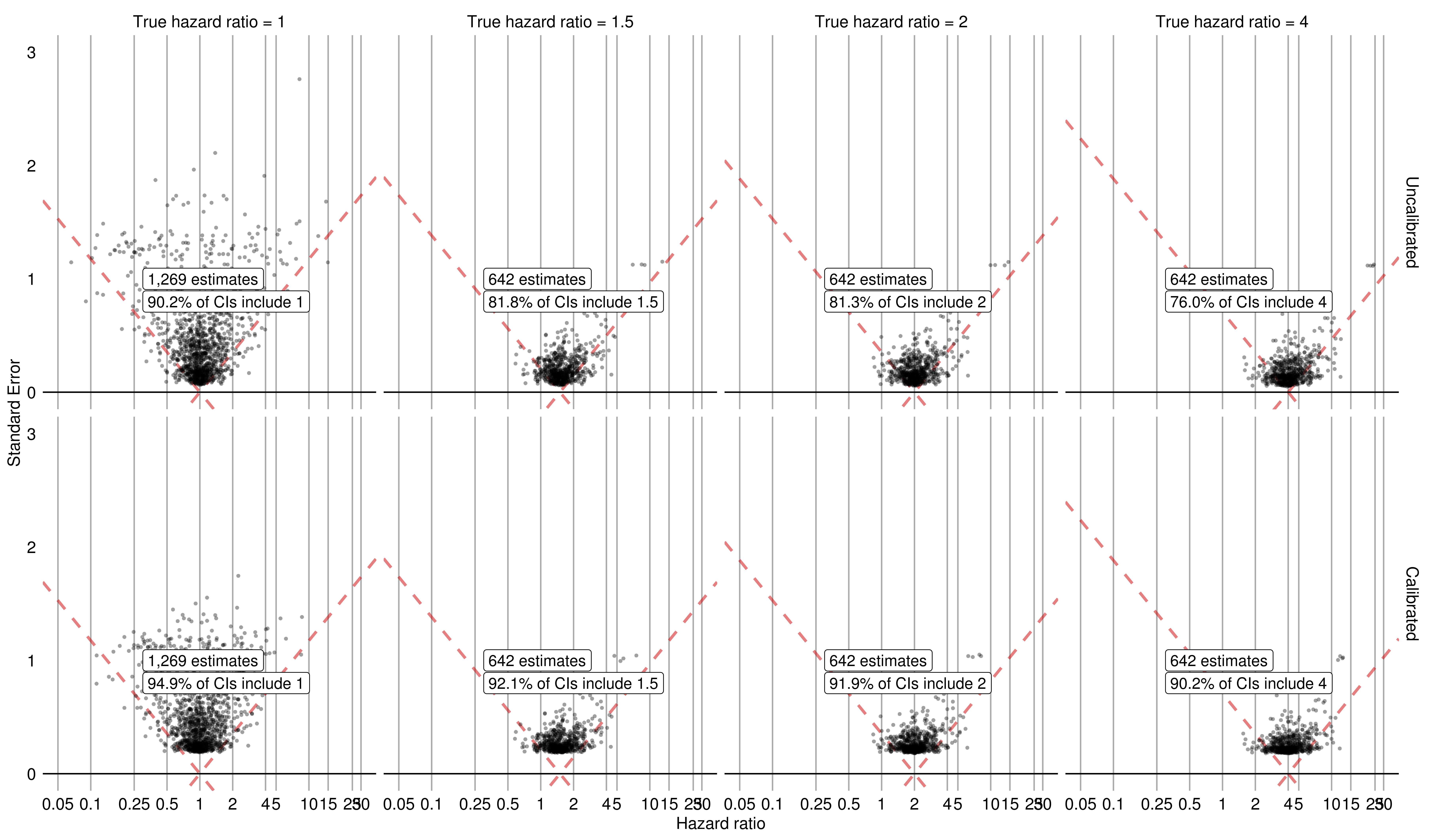
Figure 14: Evaluation of the effect estimation before (top) and after (bottom) calibration using the MDCR database in the depression data set. The linear model of bias was used and training was performed on both negative and positive controls.

We review the results of the linear model of the true bias. Figures 5, 12, 13, and 14 report effect size estimates for all negative and positive controls across the four databases as well as the percentage of posterior intervals containing the true effect size. The number of effect sizes that were tested are reported on the figures. For all four databases, the calibrated procedure results in posterior intervals that are closer to 95% than the uncalibrated procedure. In addition, for most of the cases, the constant model of the true bias performed slightly better than the linear model for the calibrated procedure.

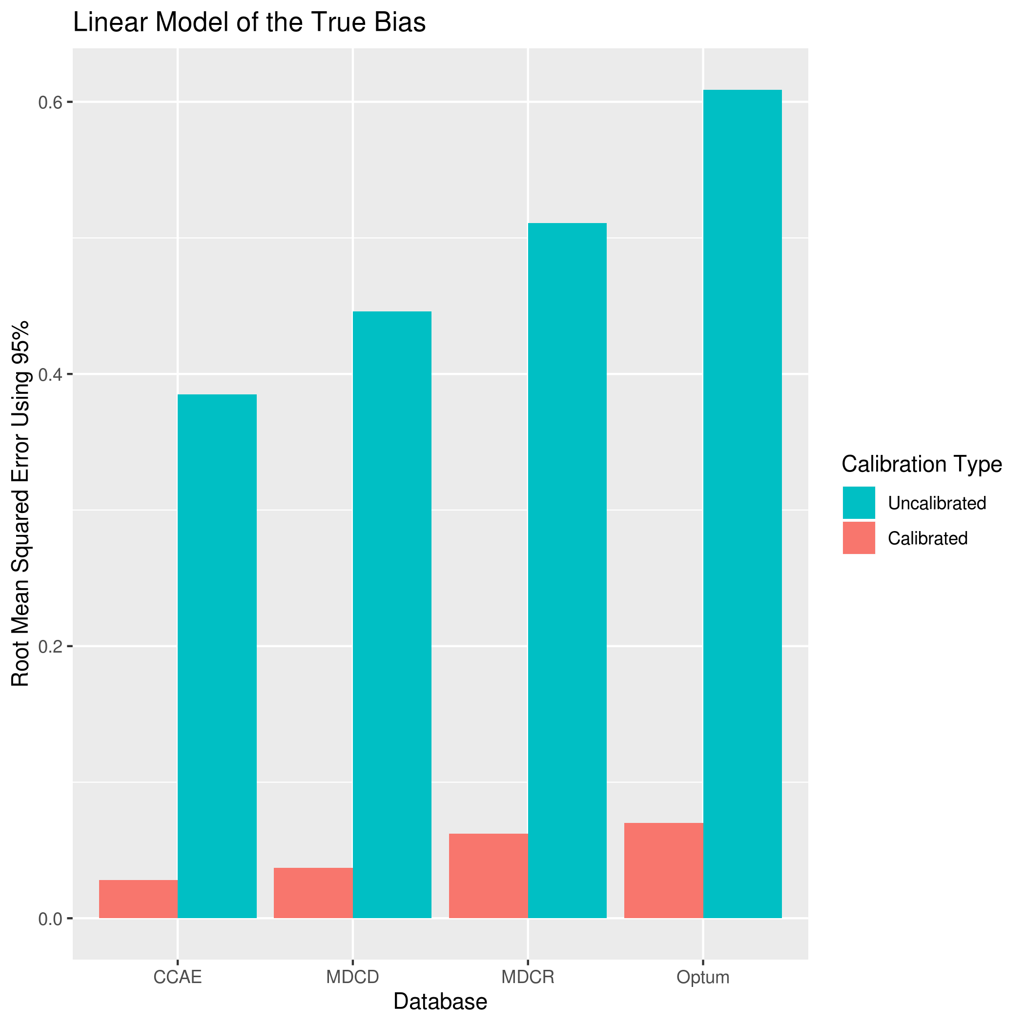
Figure 17: Root mean squared error of all effects before (uncalibrated) and after (calibrated) calibration for each of the databases in the depression data set. The linear model of bias was used and training was performed on both negative and positive controls.

The RMSE for the Optum database using calibration is about 0.07 while without calibration, it is about 0.61. Figure 17 shows the RMSE calculated for each database. The uncalibrated procedure has higher error than the calibrated procedure, when considering all hazard ratios combined.

The coverage for the calibrated and uncalibrated methods using the depression data set is displayed in Table 2.

Figure 5: Evaluation of the effect estimation before (top) and after (bottom) calibration using the Optum database in the depression data set. The linear model of bias was used and training was performed on both negative and positive controls.

3.2 Hypertension

We compare the calibrated confidence intervals using our proposed procedure to the confidence intervals generated by the gold standard, propensity score stratification. We estimate 95% posterior intervals and validate the proposed method on a data set for hypertension treatment. We use the same training and testing procedure, as well as the MCMC procedure, as used for the depression data set. The trace, histogram, empirical cumulative distribution function, and autocorrelation plots all show convergence of the variables.

3.2.1 Constant Model of the True Bias

We first consider the results for the constant model of the true bias.

Train on Negative and Positive Controls

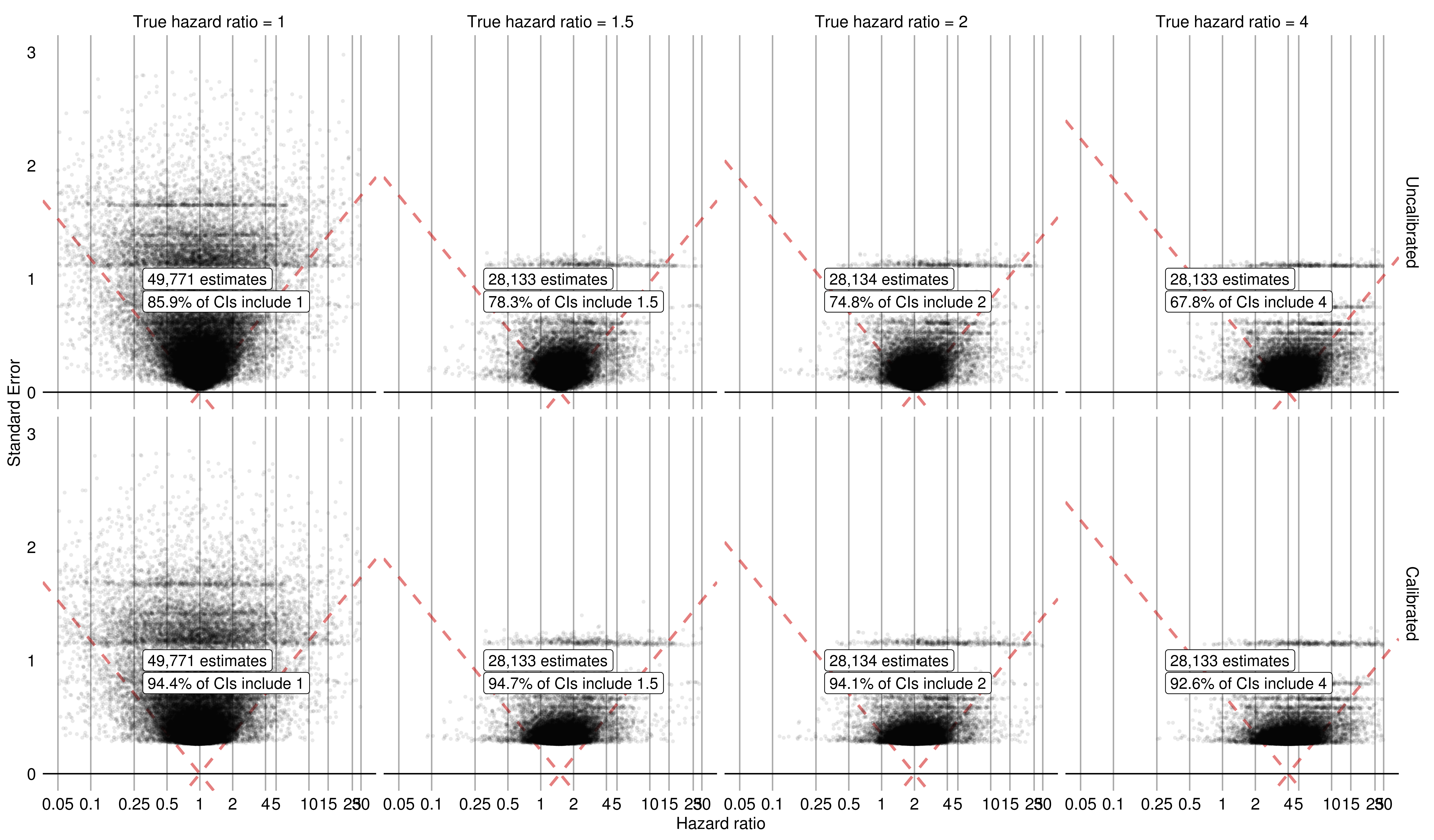
Figure 18: Evaluation of the effect estimation before (top) and after (bottom) calibration using the Optum database in the hypertension data set. The constant model of bias was used and training was performed on both negative and positive controls.

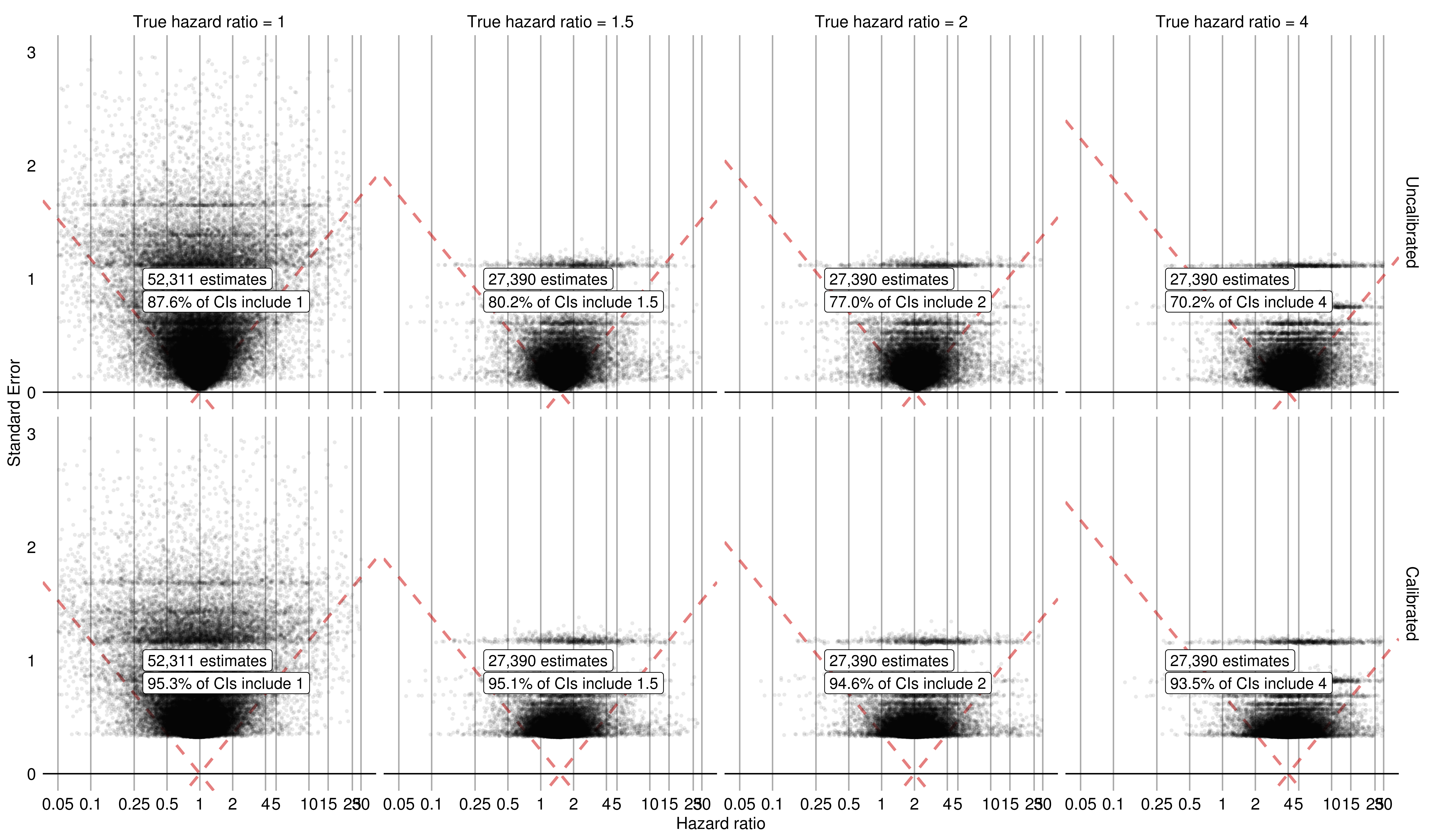
Figure 19: Evaluation of the effect estimation before (top) and after (bottom) calibration using the CCAE database in the hypertension data set. The constant model of bias was used and training was performed on both negative and positive controls.

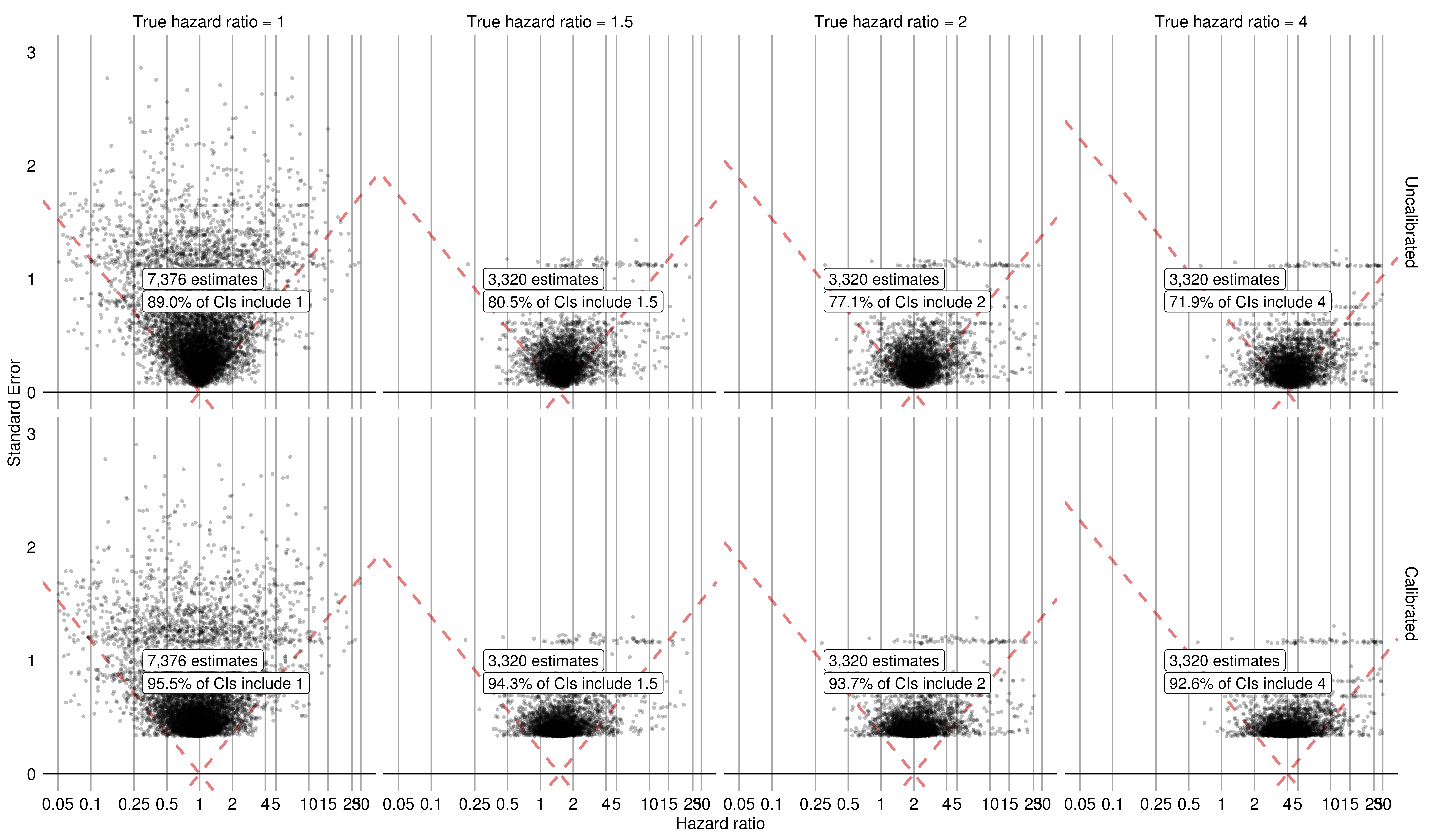
Figure 20: Evaluation of the effect estimation before (top) and after (bottom) calibration using the MDCD database in the hypertension data set. The constant model of bias was used and training was performed on both negative and positive controls.

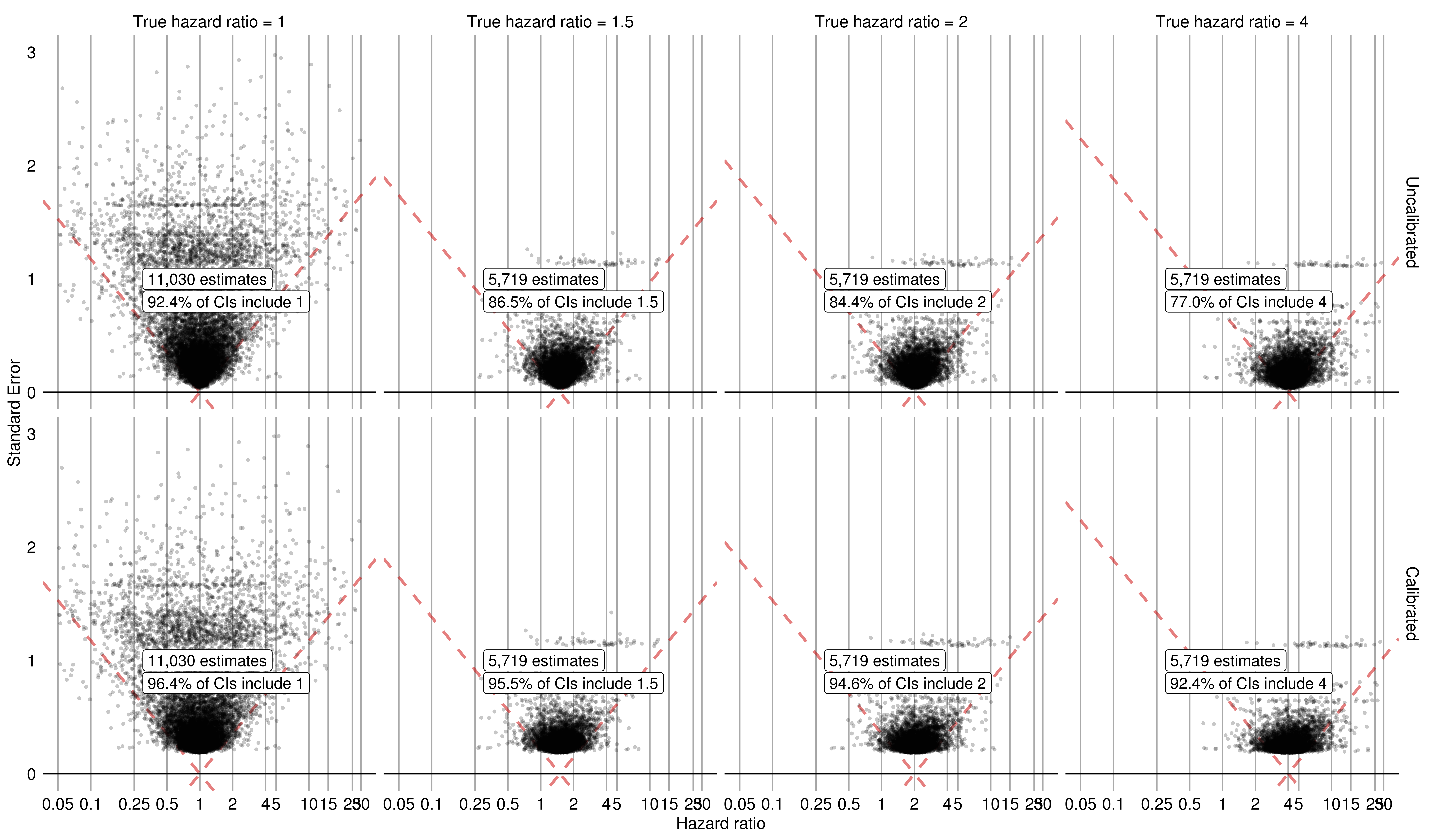
Figure 21: Evaluation of the effect estimation before (top) and after (bottom) calibration using the MDCR database in the hypertension data set. The constant model of bias was used and training was performed on both negative and positive controls.

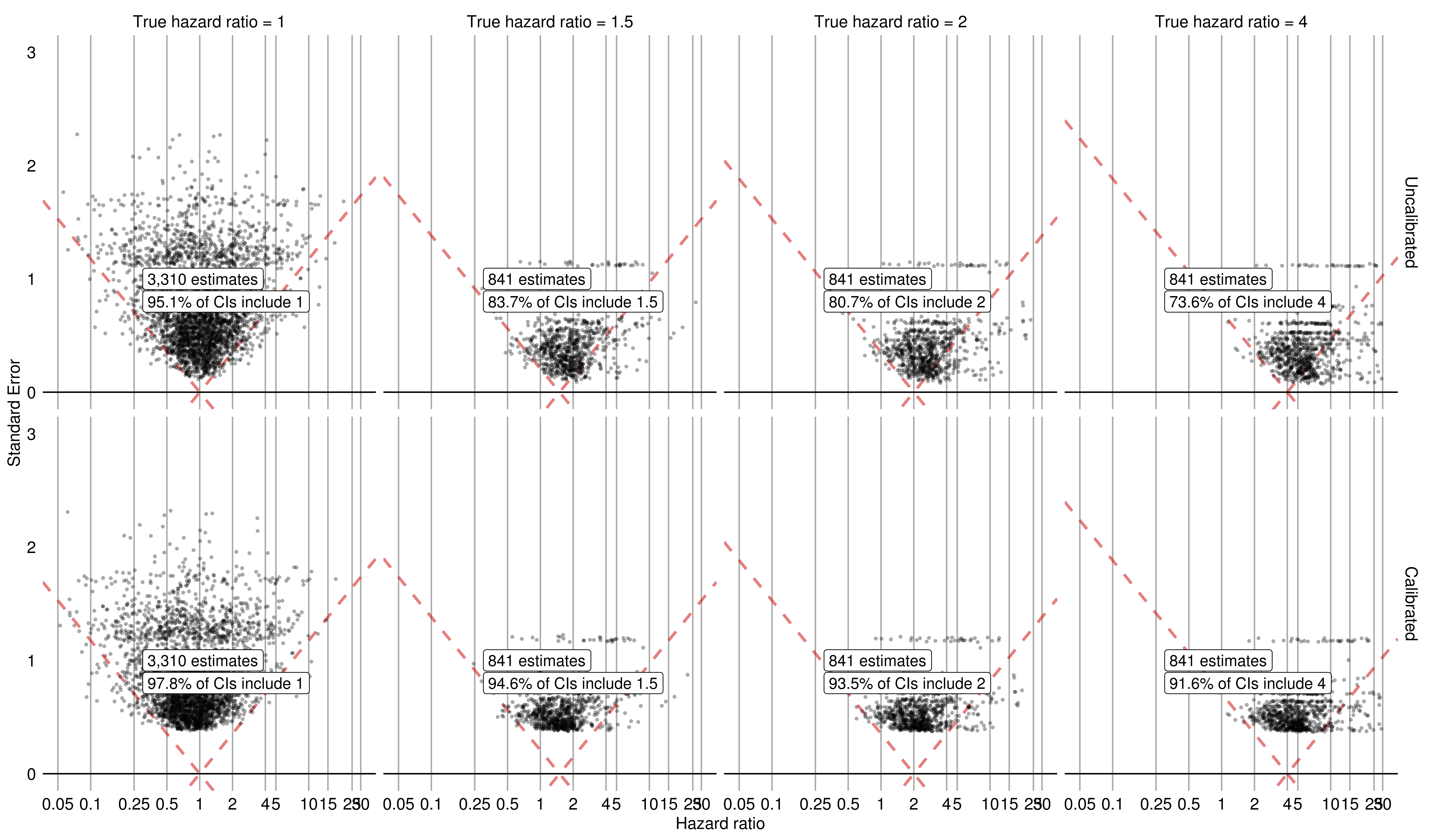
Figure 22: Evaluation of the effect estimation before (top) and after (bottom) calibration using the IMSG database in the hypertension data set. The constant model of bias was used and training was performed on both negative and positive controls.

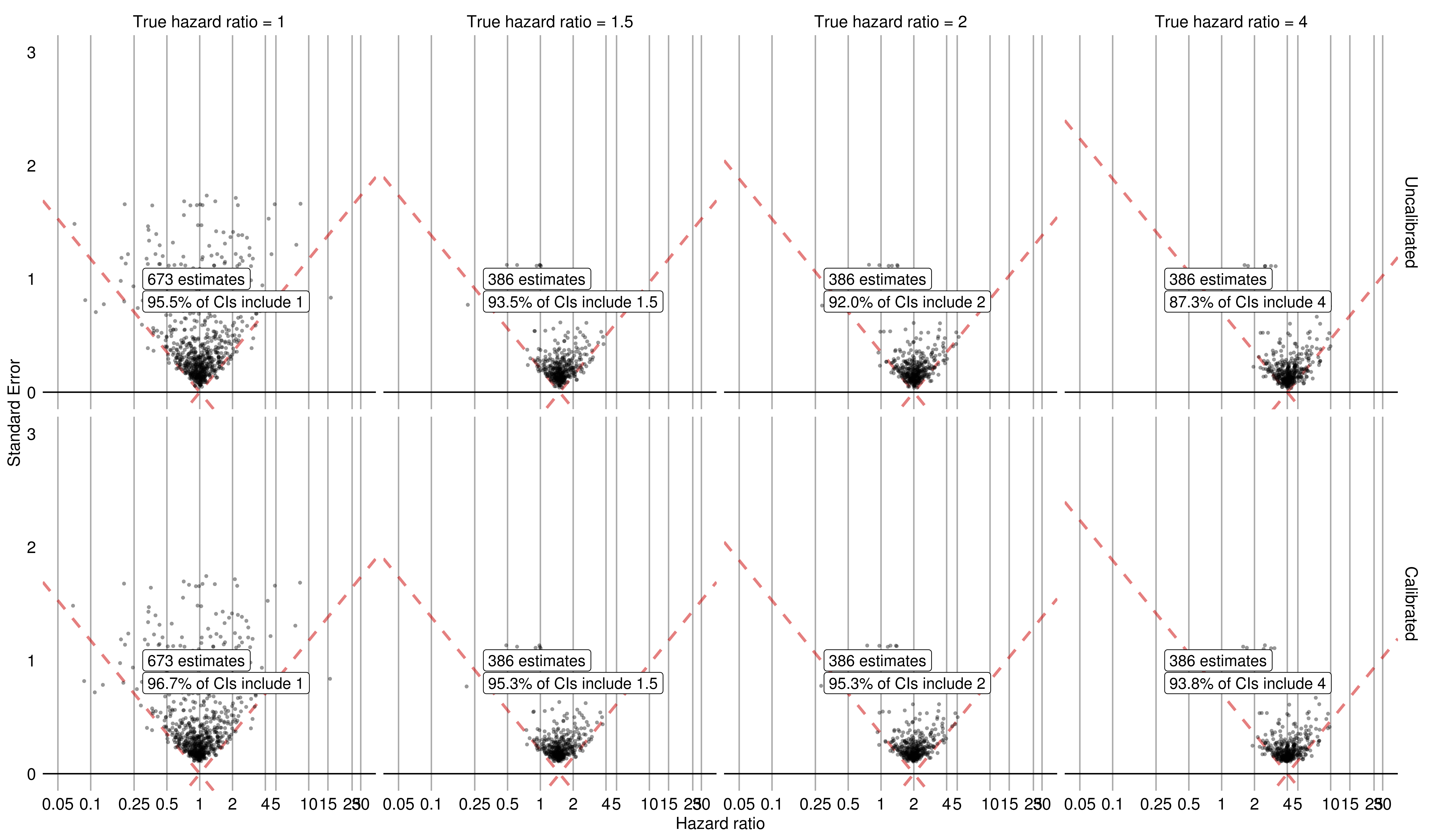
Figure 23: Evaluation of the effect estimation before (top) and after (bottom) calibration using the JMDC database in the hypertension data set. The constant model of bias was used and training was performed on both negative and positive controls.

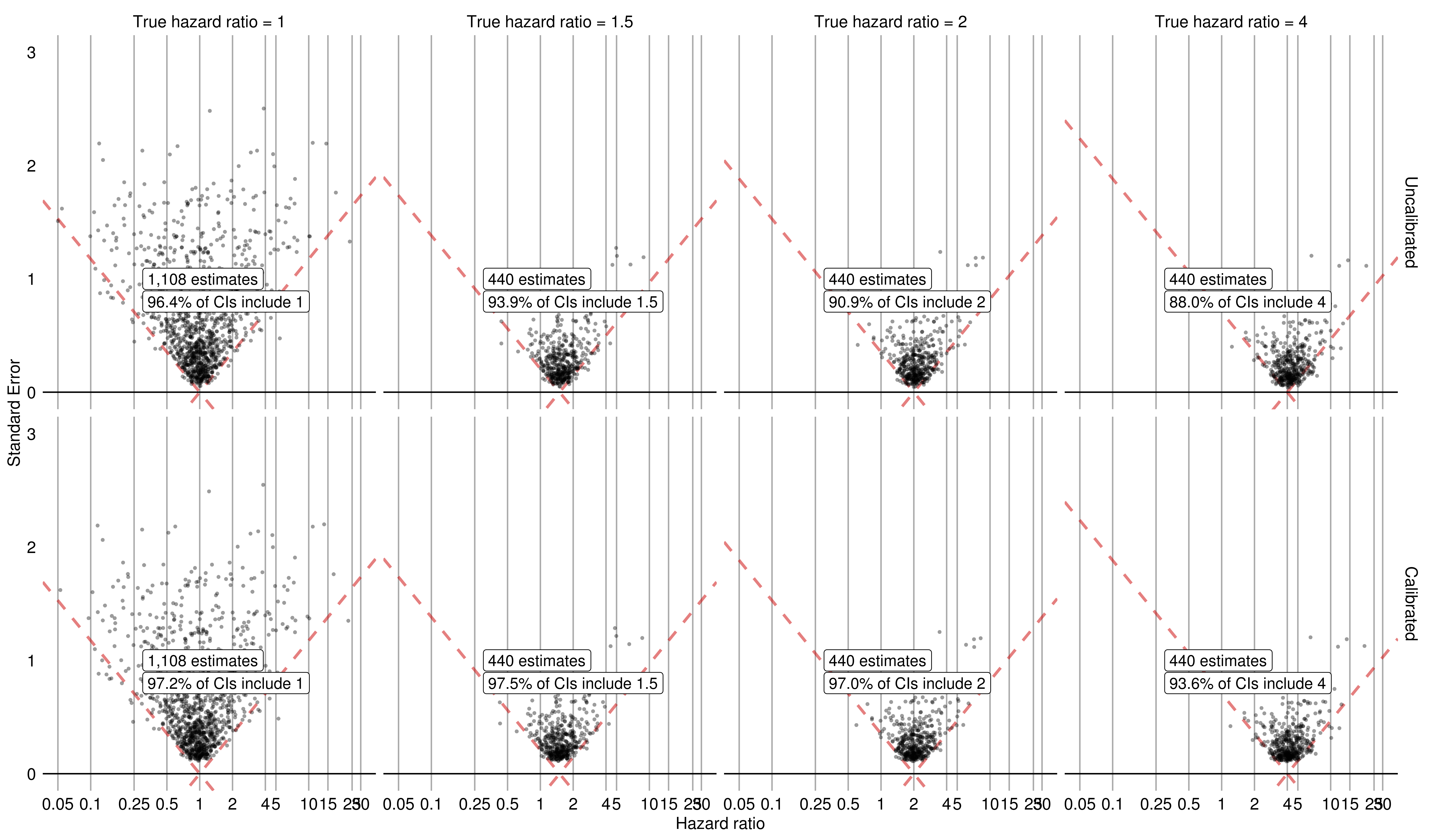
Figure 24: Evaluation of the effect estimation before (top) and after (bottom) calibration using the NHIS NSC database in the hypertension data set. The constant model of bias was used and training was performed on both negative and positive controls.

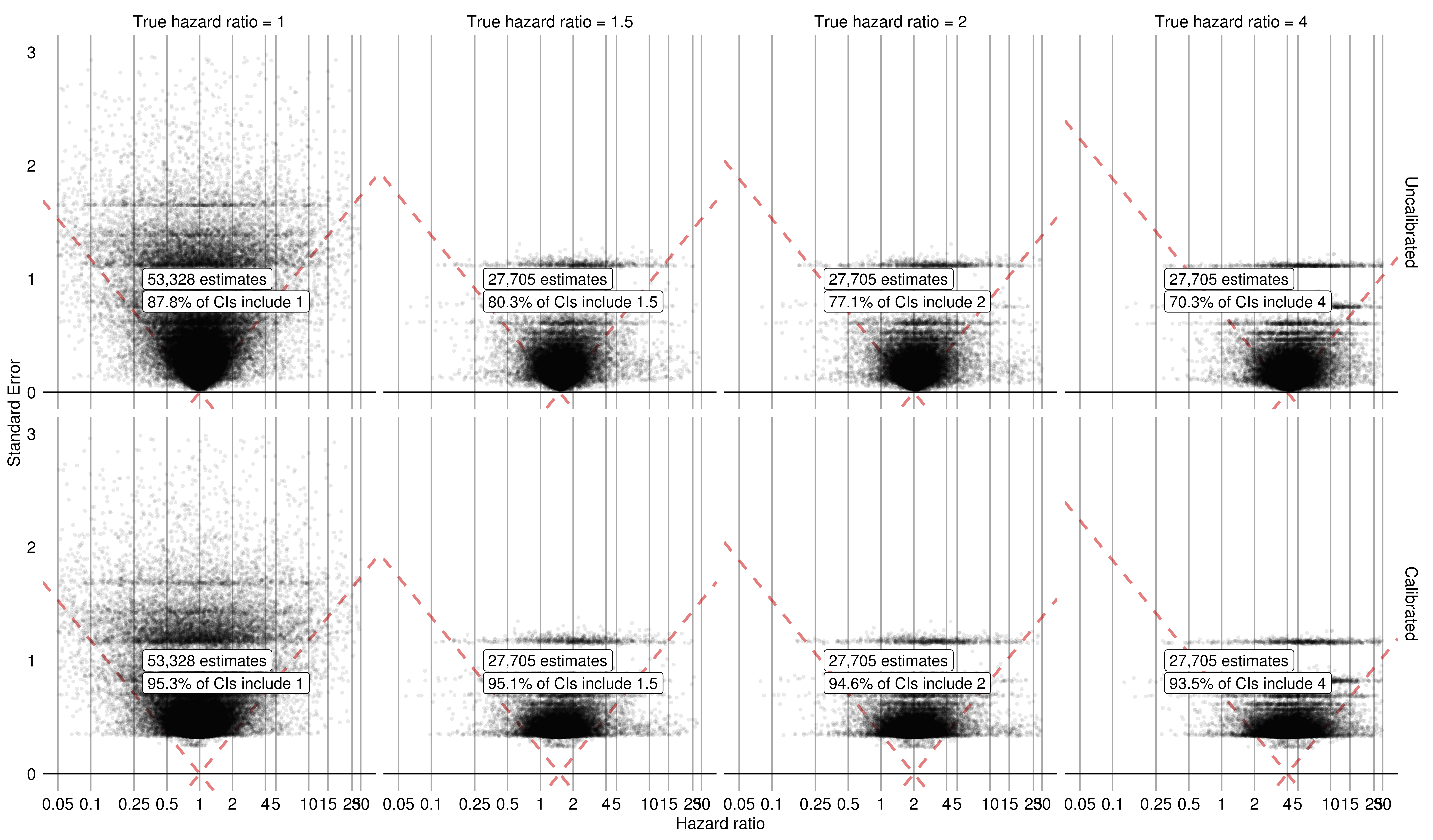
Figure 25: Evaluation of the effect estimation before (top) and after (bottom) calibration using the CUMC database in the hypertension data set. The constant model of bias was used and training was performed on both negative and positive controls.

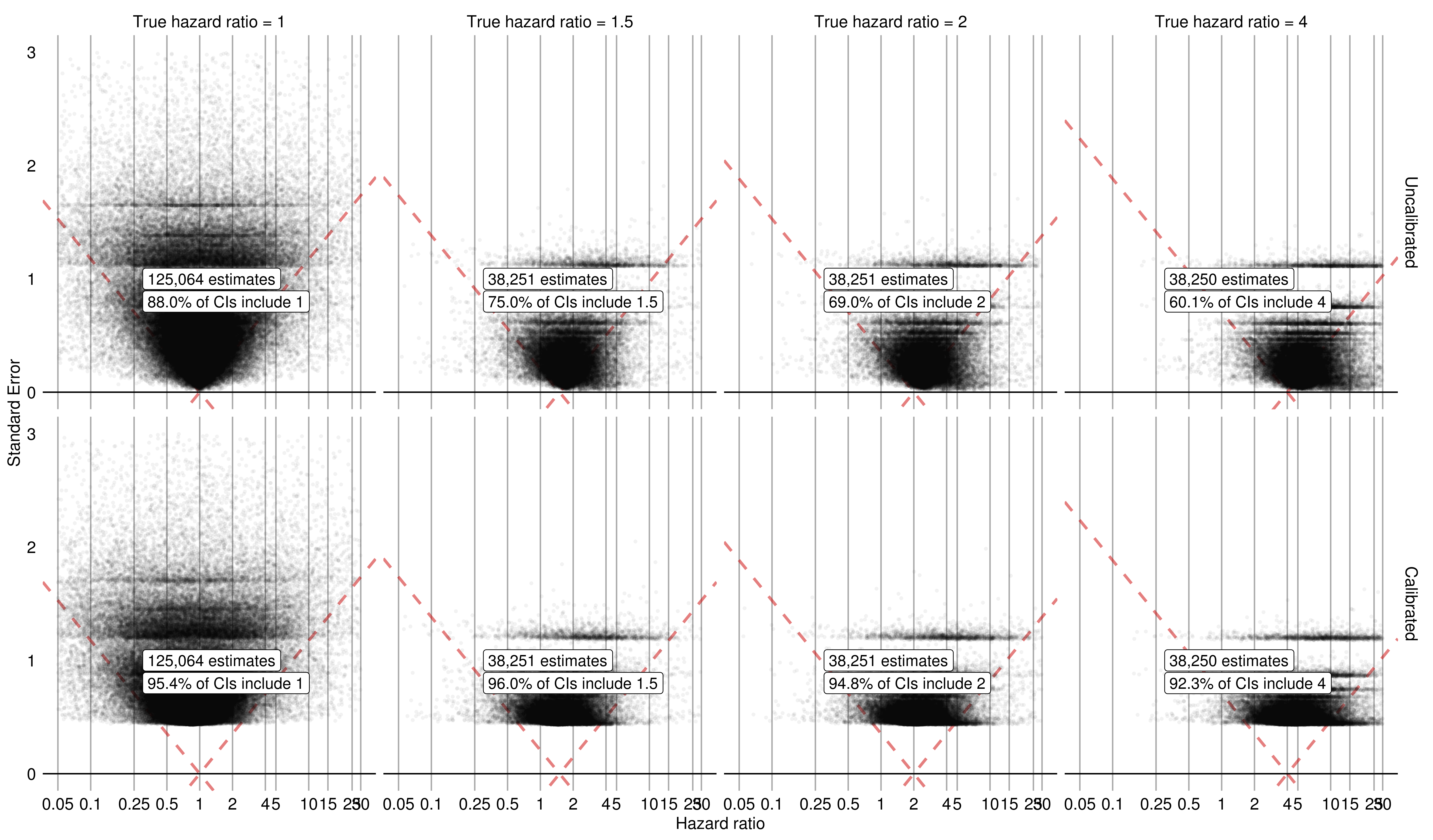
Figure 26: Evaluation of the effect estimation before (top) and after (bottom) calibration using the Panther database in the hypertension data set. The constant model of bias was used and training was performed on both negative and positive controls.

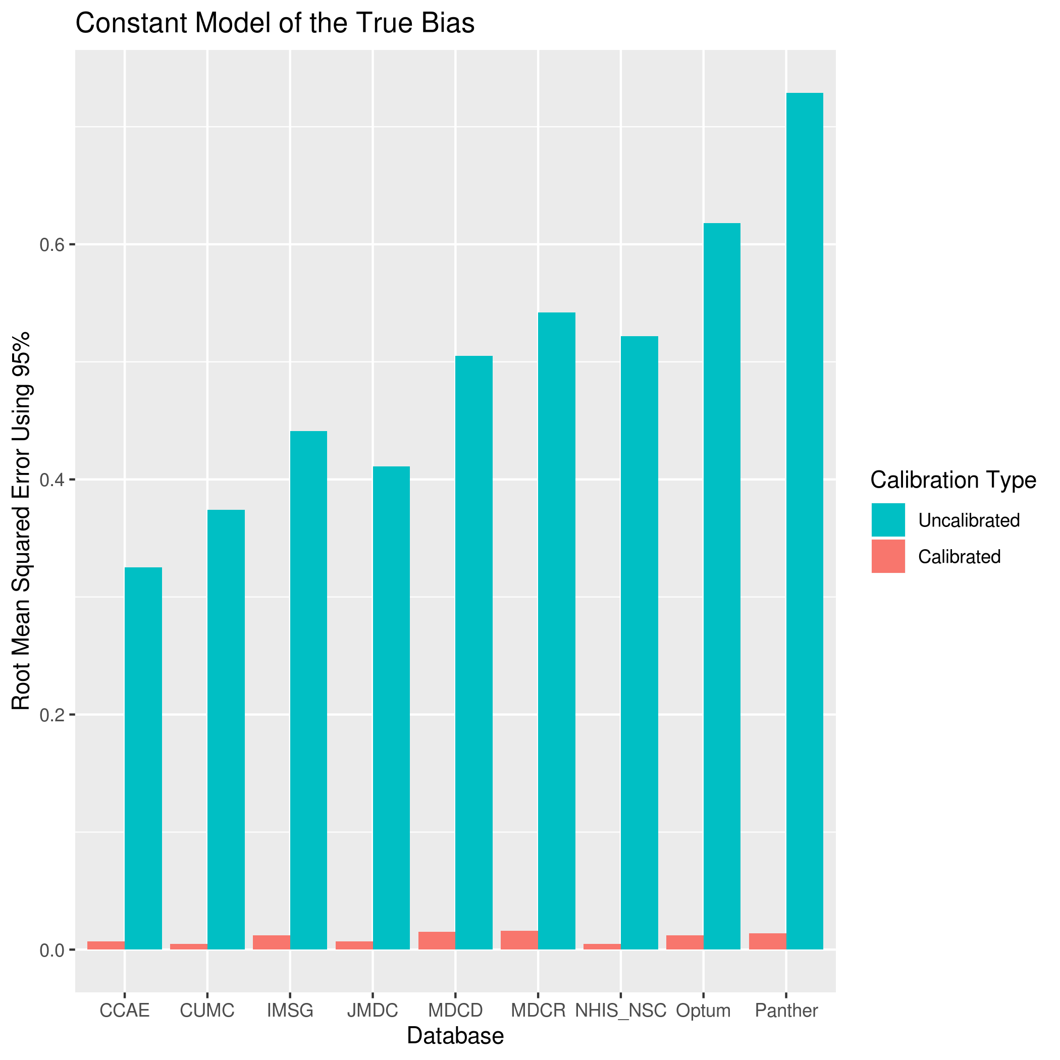
Figure 45: Root mean squared error of all effects before (uncalibrated) and after (calibrated) calibration for each of the nine databases in the hypertension data set. The constant model of bias was used and training was performed on both negative and positive controls.

We train on both negative and positive controls. Figures 18, 19, 20, 21, 22, 23, 24, 25, and 26 report effect size estimates for all negative and positive controls for the nine databases as well as the percentage of posterior intervals containing the true effect size. The number of effect sizes that were tested are reported on the figures. For Optum, CCAE, MDCD, MDCR, and Panther, the calibrated procedure results in posterior intervals that are closer to 95% than the uncalibrated procedure. However, the other five databases had varying results. For the CUMC, JMDC, and IMSG databases, for the hazard ratio of one, the uncalibrated procedure performed slightly better than the calibrated procedure. For the other hazard ratios, the calibrated procedure performed better than the uncalibrated procedure. For the NHIS NSC database, the uncalibrated procedure performed slightly better for the hazard ratio of 1 and 1.5, and the calibrated procedure performed better for the hazard ratio of 2 and 4. Figure 45 shows the RMSE calculated for each database. The uncalibrated procedure has higher error than the calibrated procedure, when considering all hazard ratios combined.

Train on Only Negative Controls

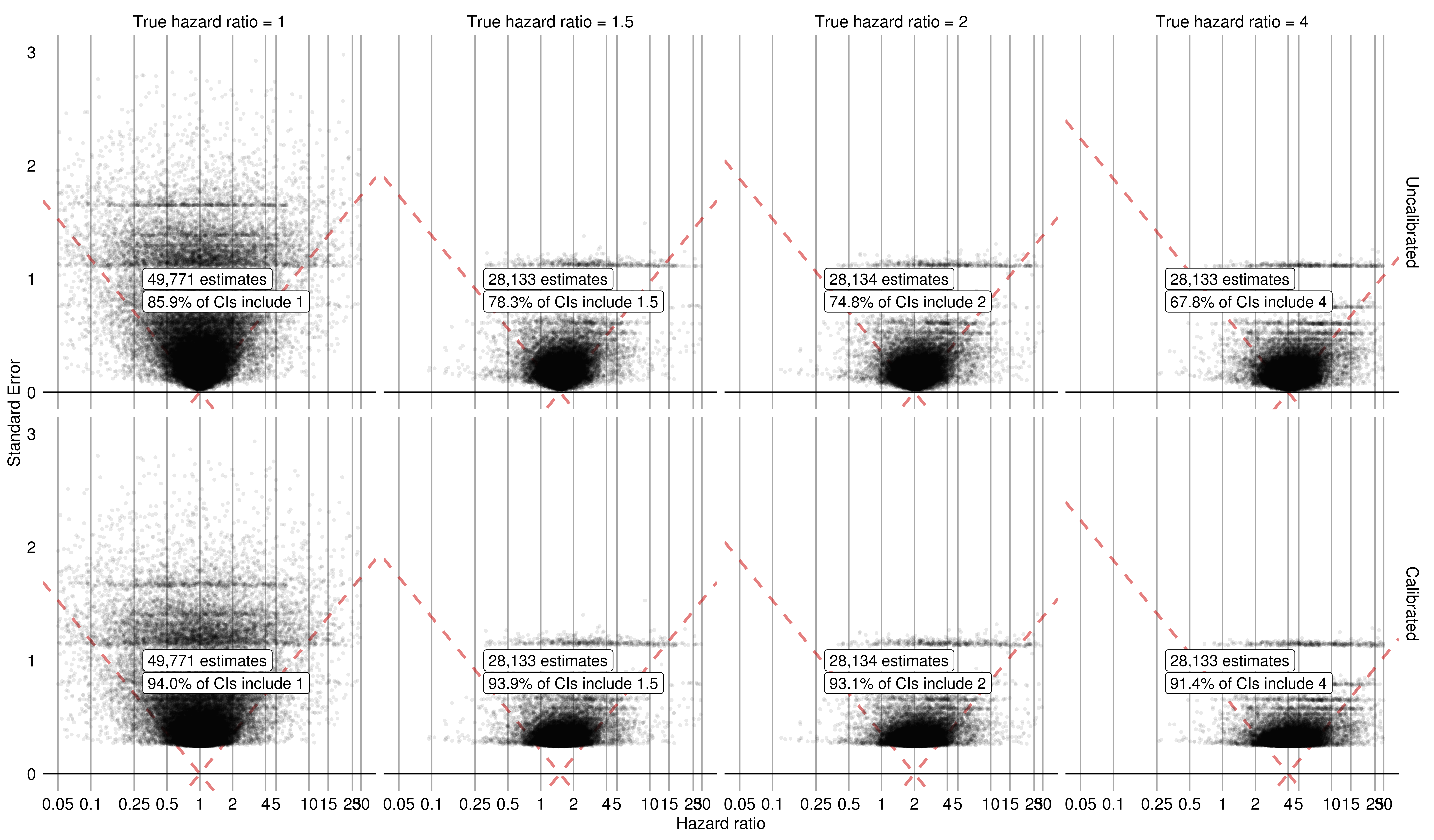
Figure 27: Evaluation of the effect estimation before (top) and after (bottom) calibration using the Optum database in the hypertension data set. The constant model of bias was used and training was performed on only negative controls.

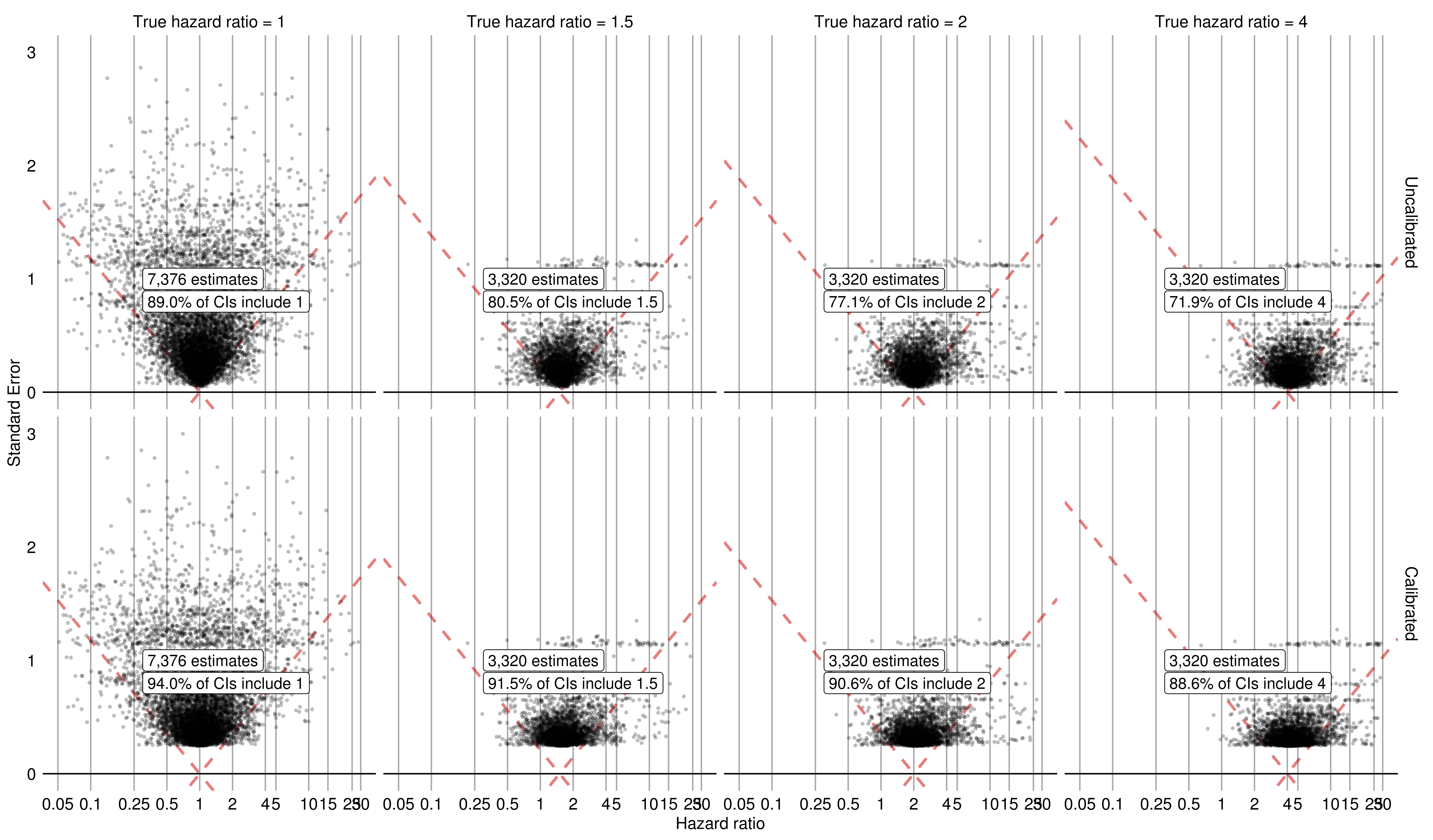
Figure 29: Evaluation of the effect estimation before (top) and after (bottom) calibration using the MDCD database in the hypertension data set. The constant model of bias was used and training was performed on only negative controls.

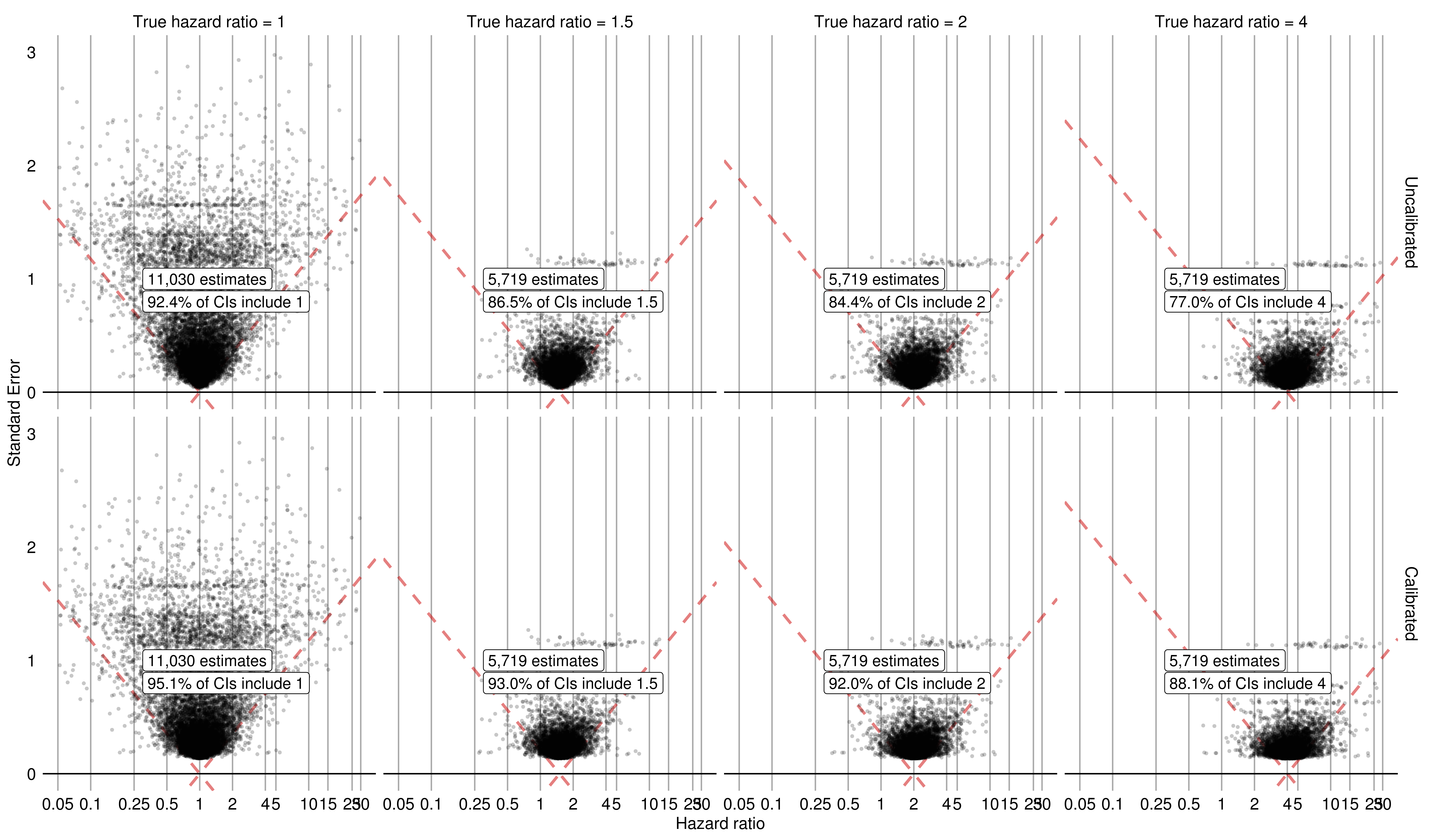
Figure 30: Evaluation of the effect estimation before (top) and after (bottom) calibration using the MDCR database in the hypertension data set. The constant model of bias was used and training was performed on only negative controls.

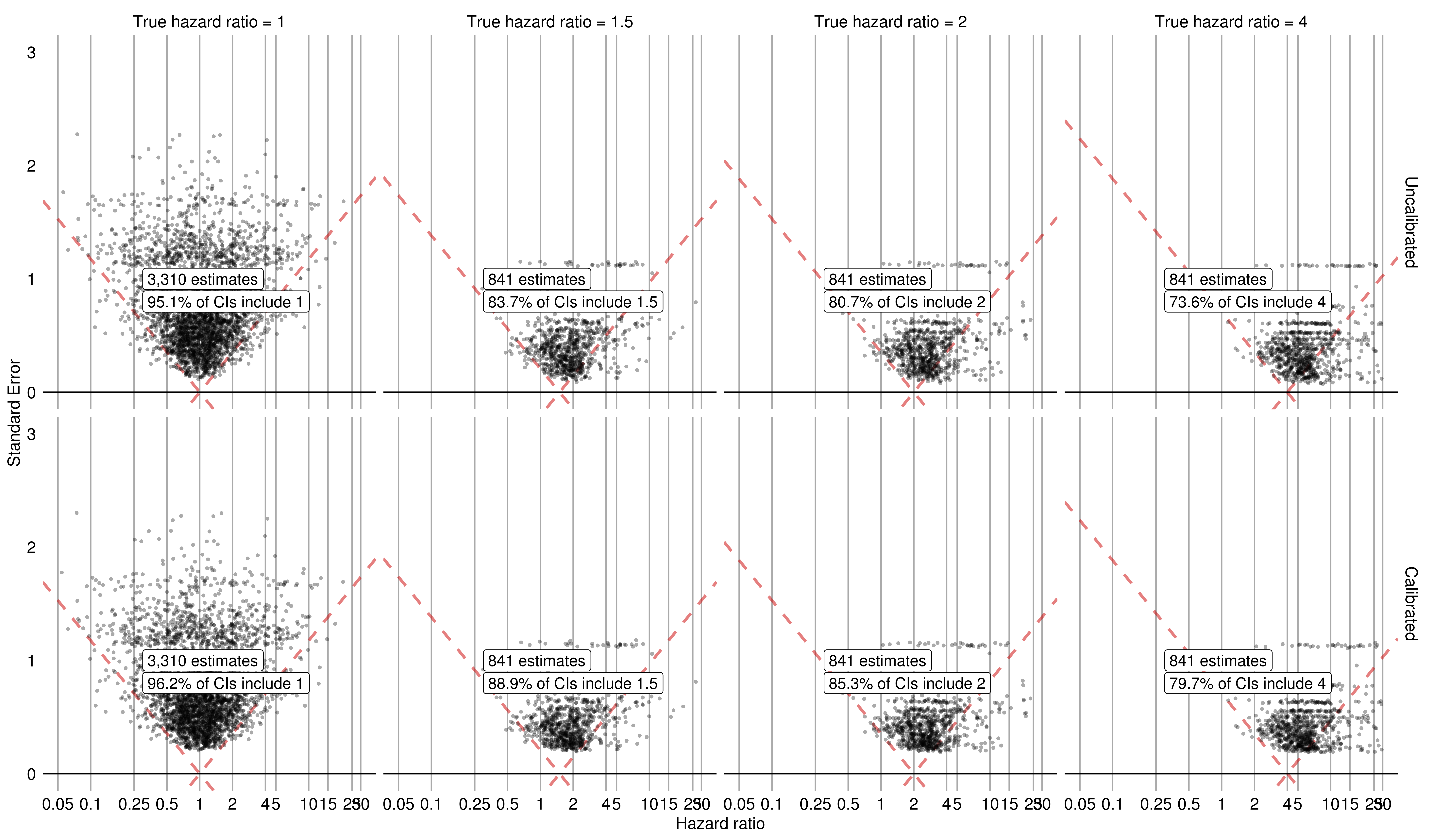
Figure 31: Evaluation of the effect estimation before (top) and after (bottom) calibration using the IMSG database in the hypertension data set. The constant model of bias was used and training was performed on only negative controls.

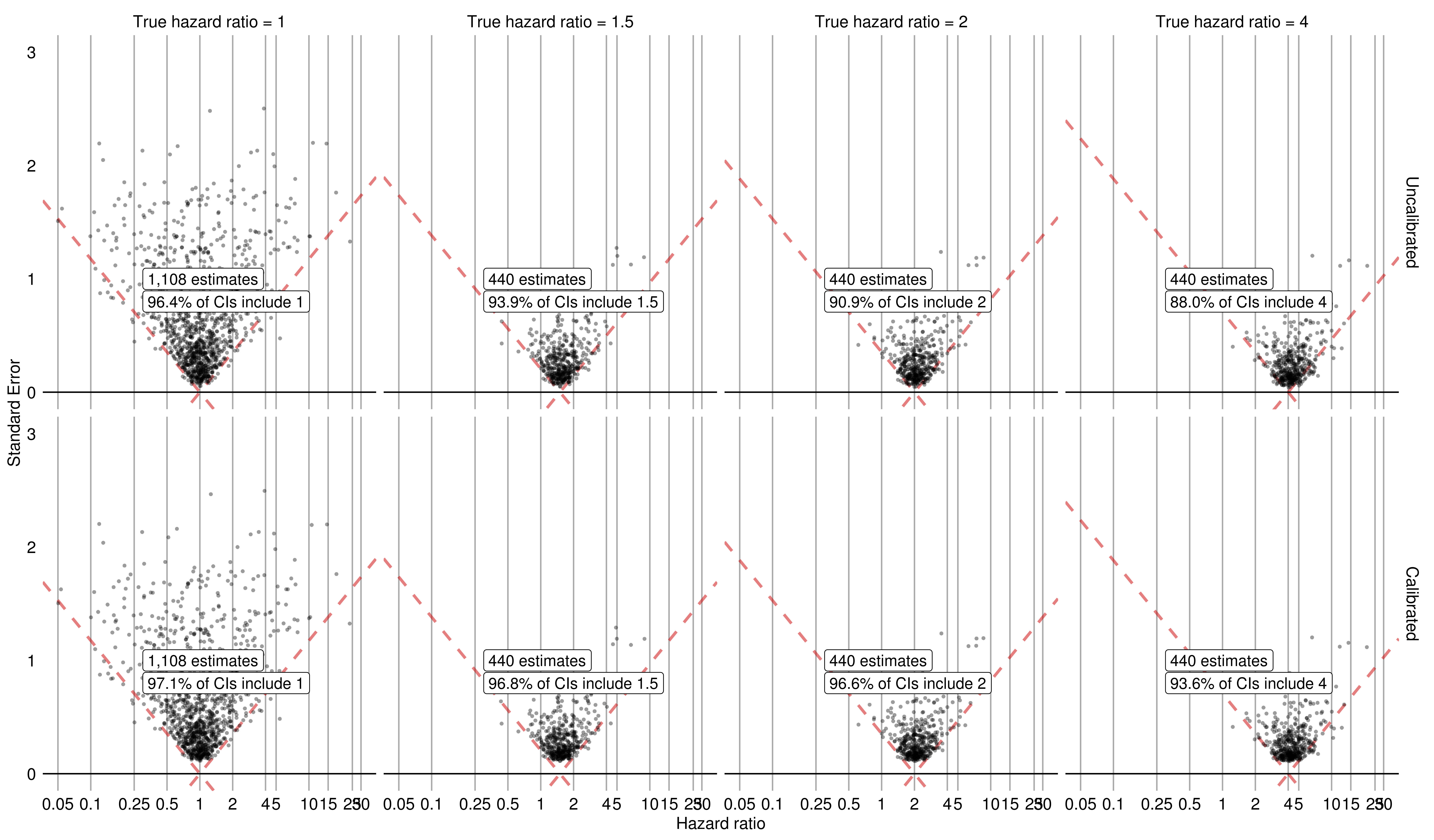
Figure 33: Evaluation of the effect estimation before (top) and after (bottom) calibration using the NHIS NSC database in the hypertension data set. The constant model of bias was used and training was performed on only negative controls.

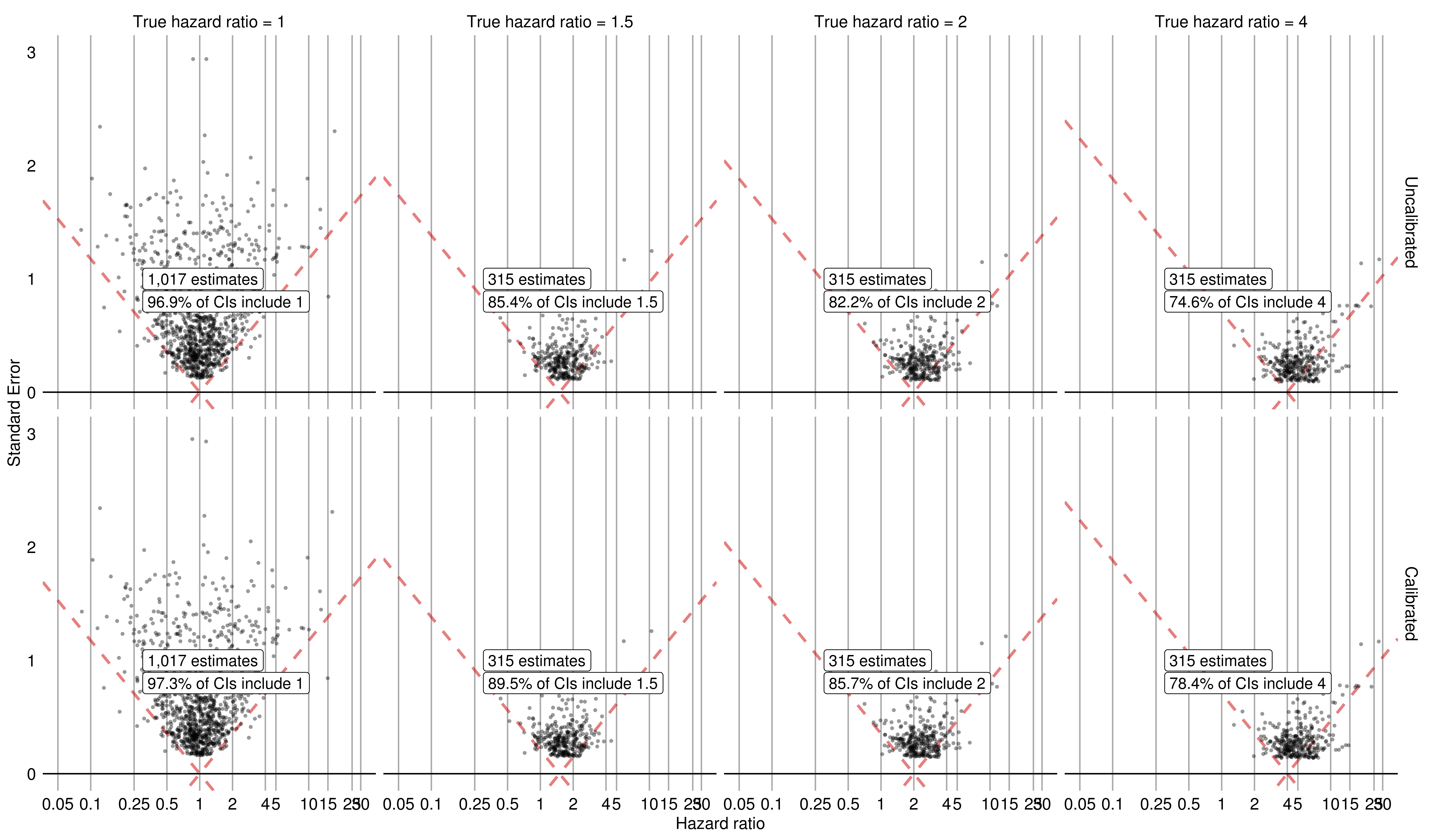
Figure 34: Evaluation of the effect estimation before (top) and after (bottom) calibration using the CUMC database in the hypertension data set. The constant model of bias was used and training was performed on only negative controls.

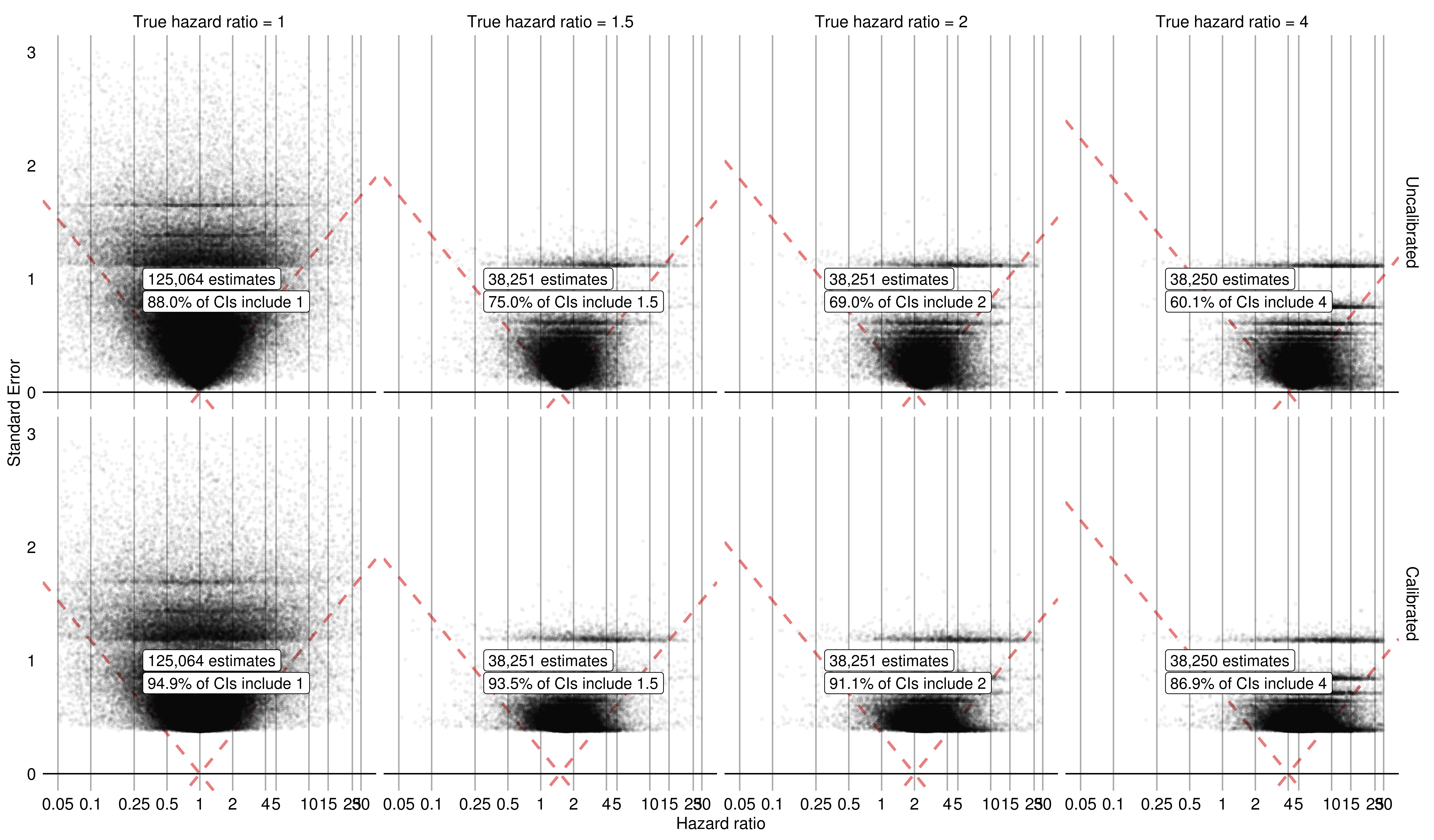
Figure 35: Evaluation of the effect estimation before (top) and after (bottom) calibration using the Panther database in the hypertension data set. The constant model of bias was used and training was performed on only negative controls.

We consider the effect of training on negative controls only. Figures 27, 28, 29, 30, 31, 32, 33, 34, and 35 report effect size estimates for all negative and positive controls across four databases (Optum, CCAE, MDCD, MDCR) as well as the percentage of posterior intervals containing the true effect size. The number of effect sizes that were tested are reported on the figures. For Optum, CCAE, MDCD, MDCR, and Panther, the calibrated procedure results in posterior intervals that are closer to 95% than the uncalibrated procedure. The other five databases had similar results to the training on negative and positive controls analysis with the constant model of the true bias. For the CUMC, JMDC, and IMSG databases, for the hazard ratio of one, the uncalibrated procedure performed slightly better than the calibrated procedure. For the other hazard ratios, the calibrated procedure performed better than the uncalibrated procedure. For the NHIS NSC database, the uncalibrated procedure performed slightly better for the hazard ratio of 1 and 1.5, and the calibrated procedure performed better for the hazard ratio of 2 and 4.

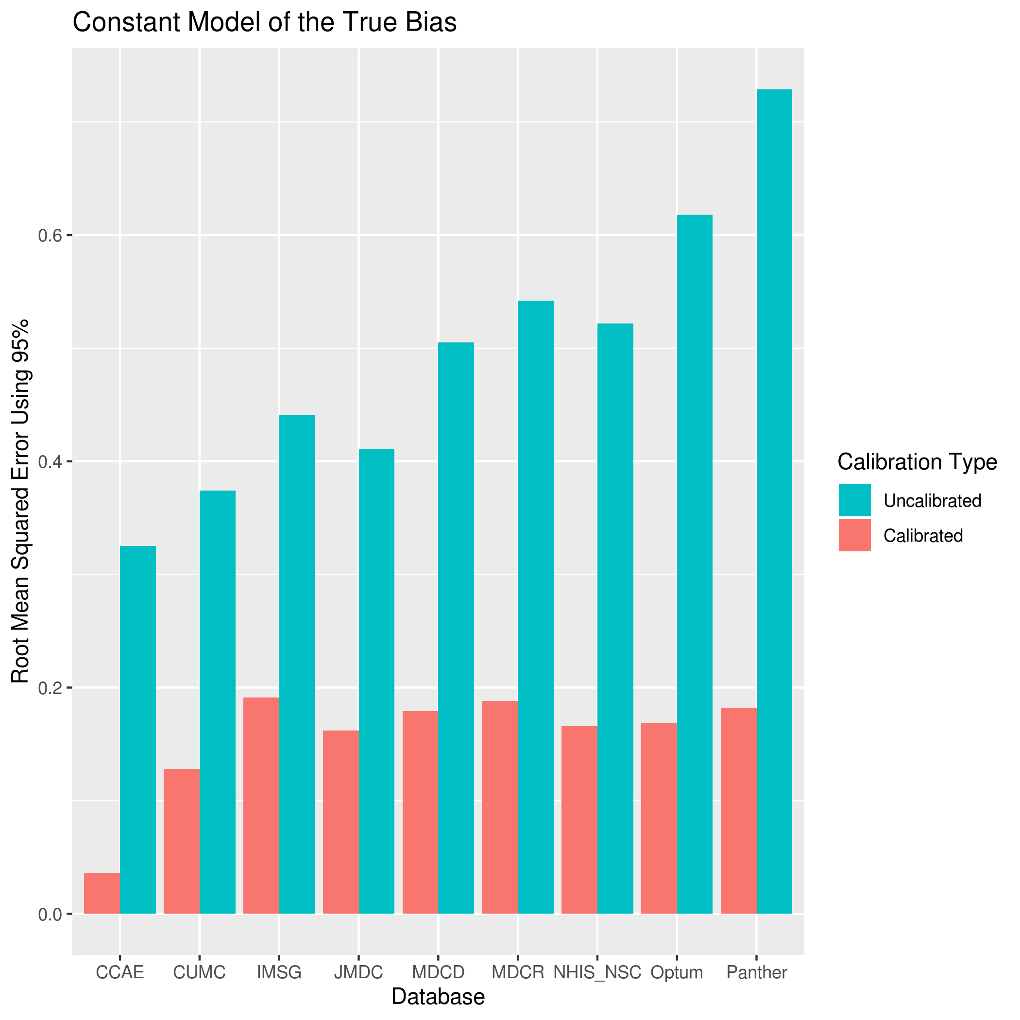
Figure 46: Root mean squared error of all effects before (uncalibrated) and after (calibrated) calibration for each of the nine databases in the hypertension data set. The constant model of bias was used and training was performed on only negative controls.

Figure 46 shows the RMSE calculated for each database. Again, the uncalibrated procedure has higher error overall than the calibrated procedure, when considering all hazard ratios combined. Interestingly, there appears to be more error overall when training on negative controls only compared to training on negative and positive controls.

3.2.2 Linear Model of the True Bias

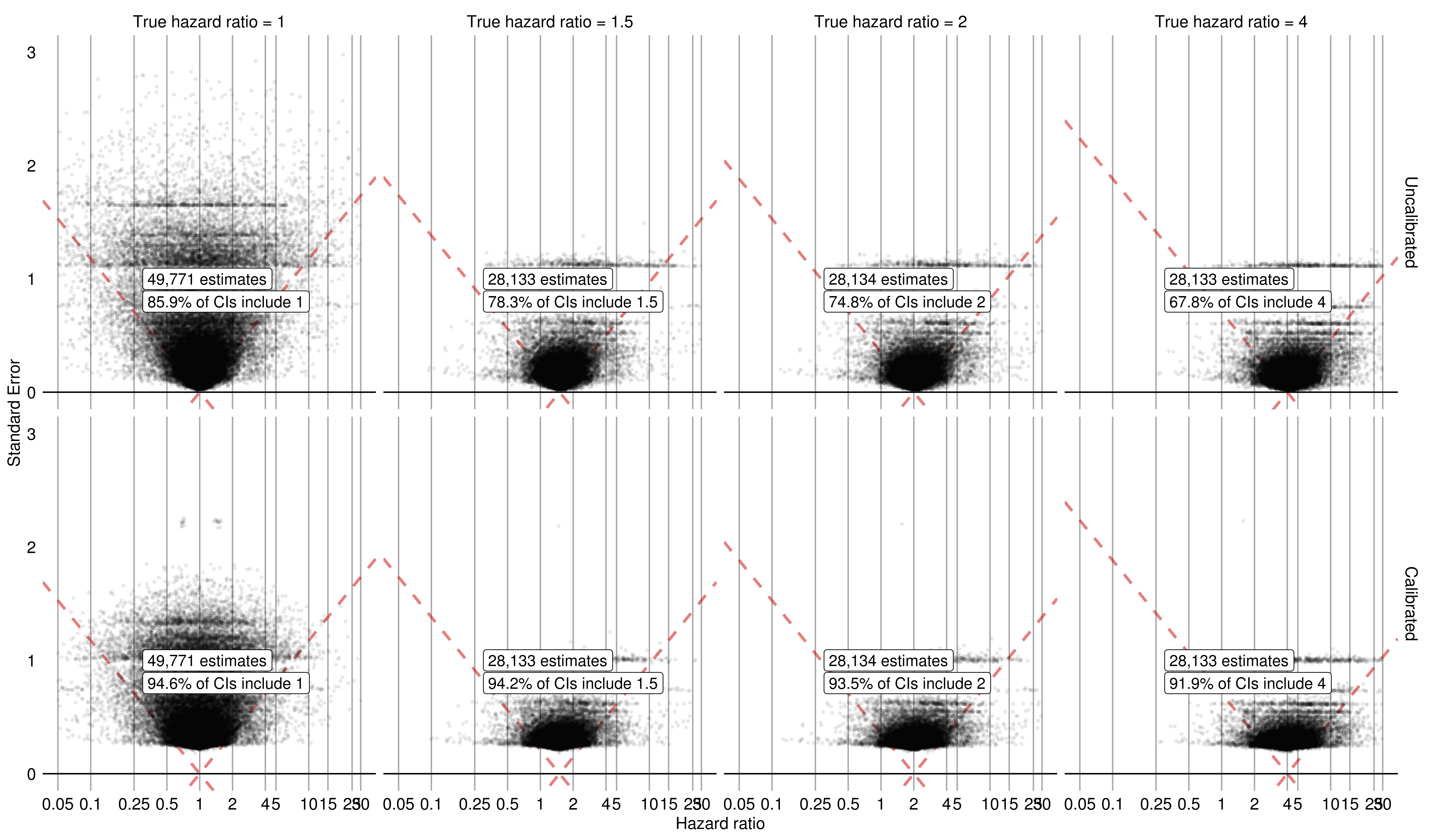
Figure 36: Evaluation of the effect estimation before (top) and after (bottom) calibration using the Optum database in the hypertension data set. The linear model of bias was used and training was performed on both negative and positive controls.

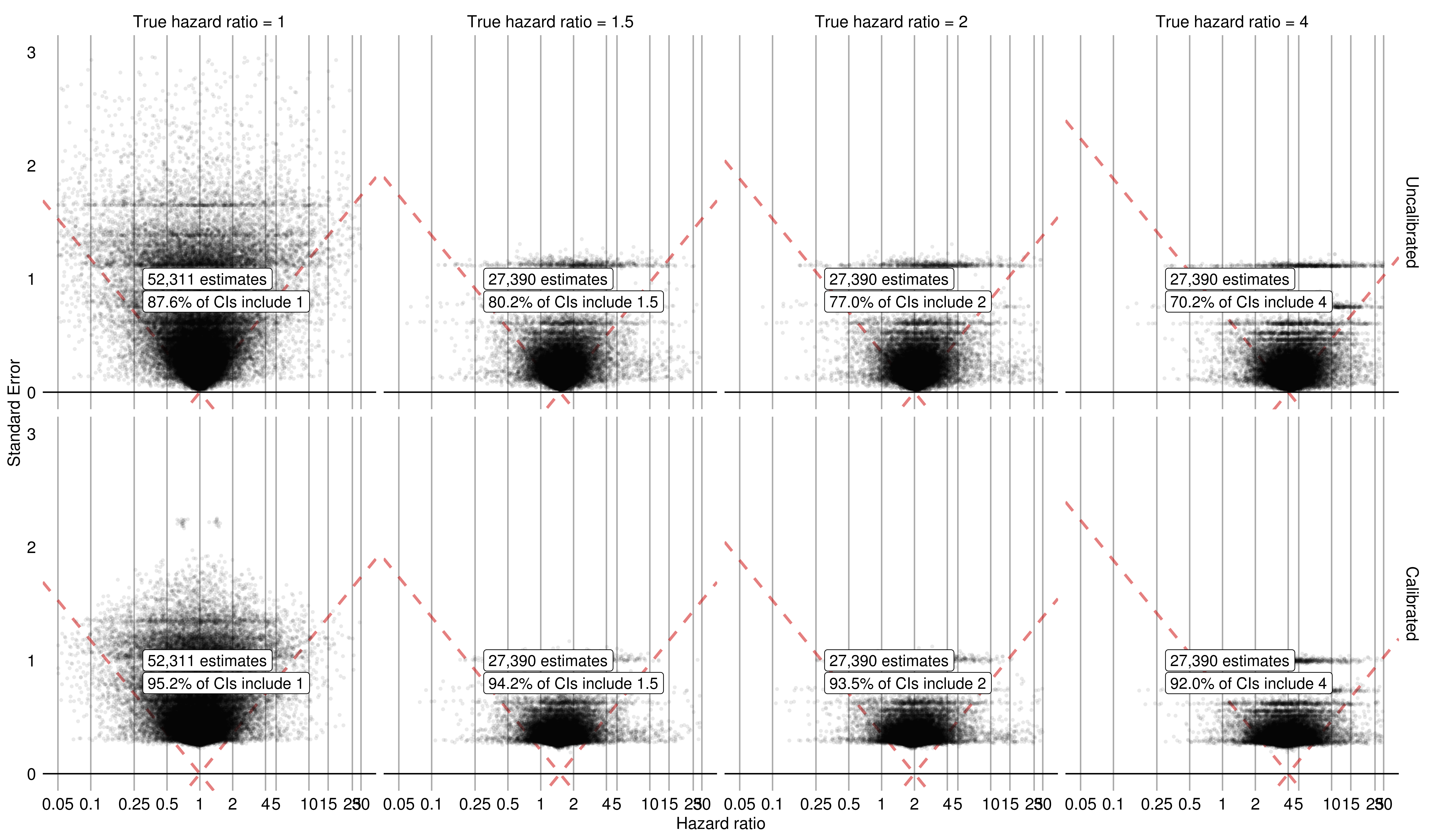
Figure 37: Evaluation of the effect estimation before (top) and after (bottom) calibration using the CCAE database in the hypertension data set. The linear model of bias was used and training was performed on both negative and positive controls.

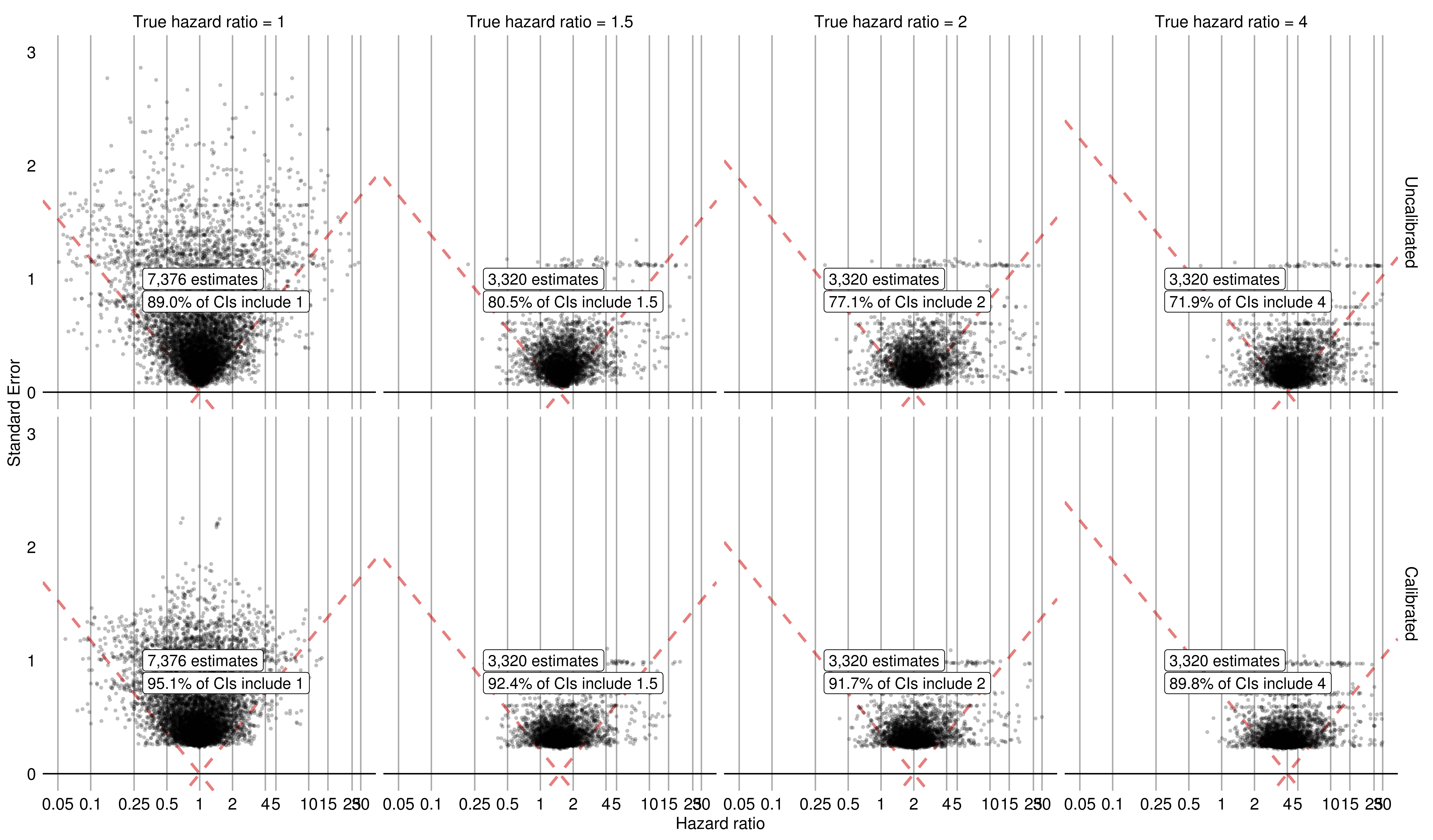
Figure 38: Evaluation of the effect estimation before (top) and after (bottom) calibration using the MDCD database in the hypertension data set. The linear model of bias was used and training was performed on both negative and positive controls.

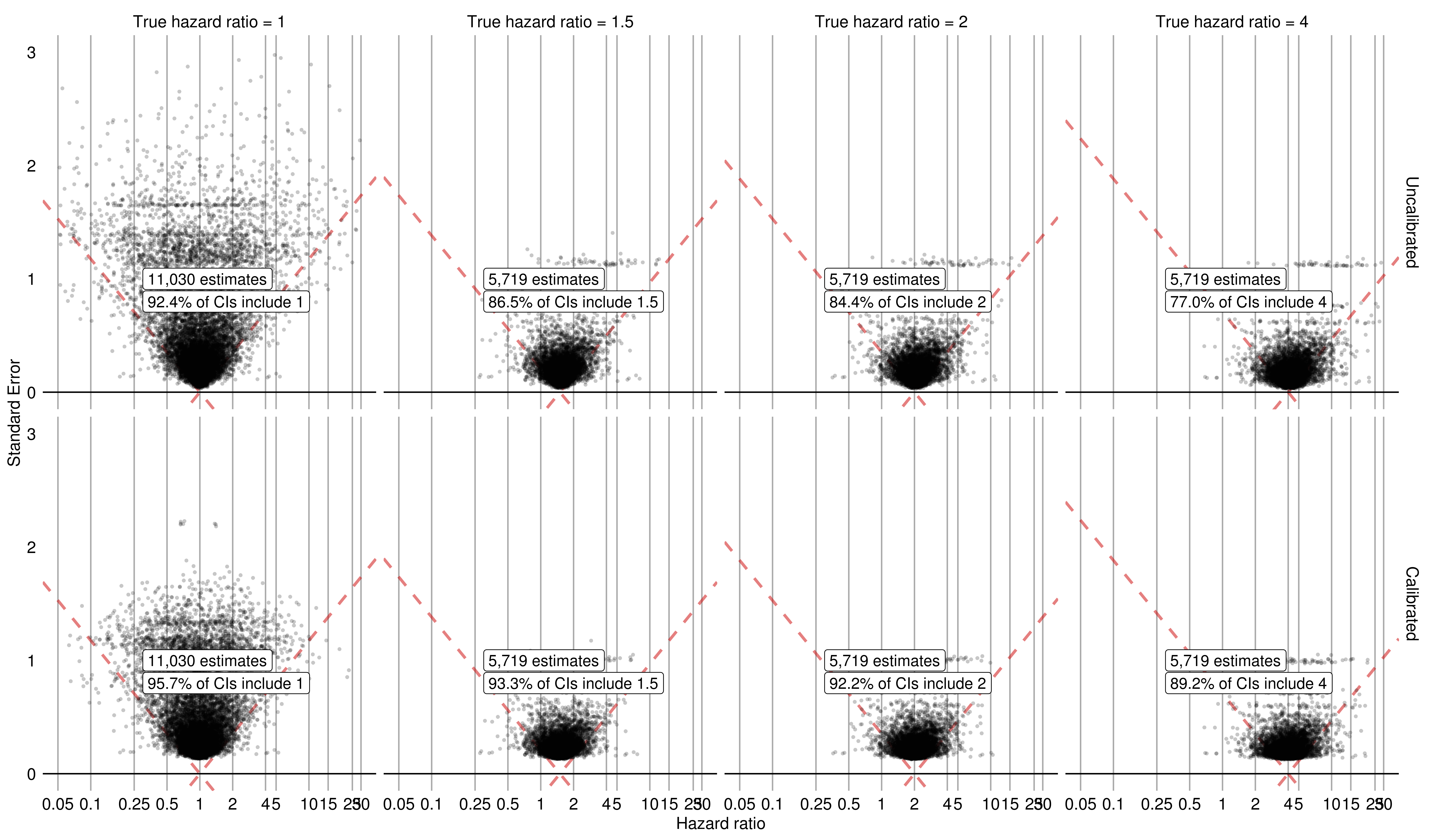
Figure 39: Evaluation of the effect estimation before (top) and after (bottom) calibration using the MDCR database in the hypertension data set. The linear model of bias was used and training was performed on both negative and positive controls.

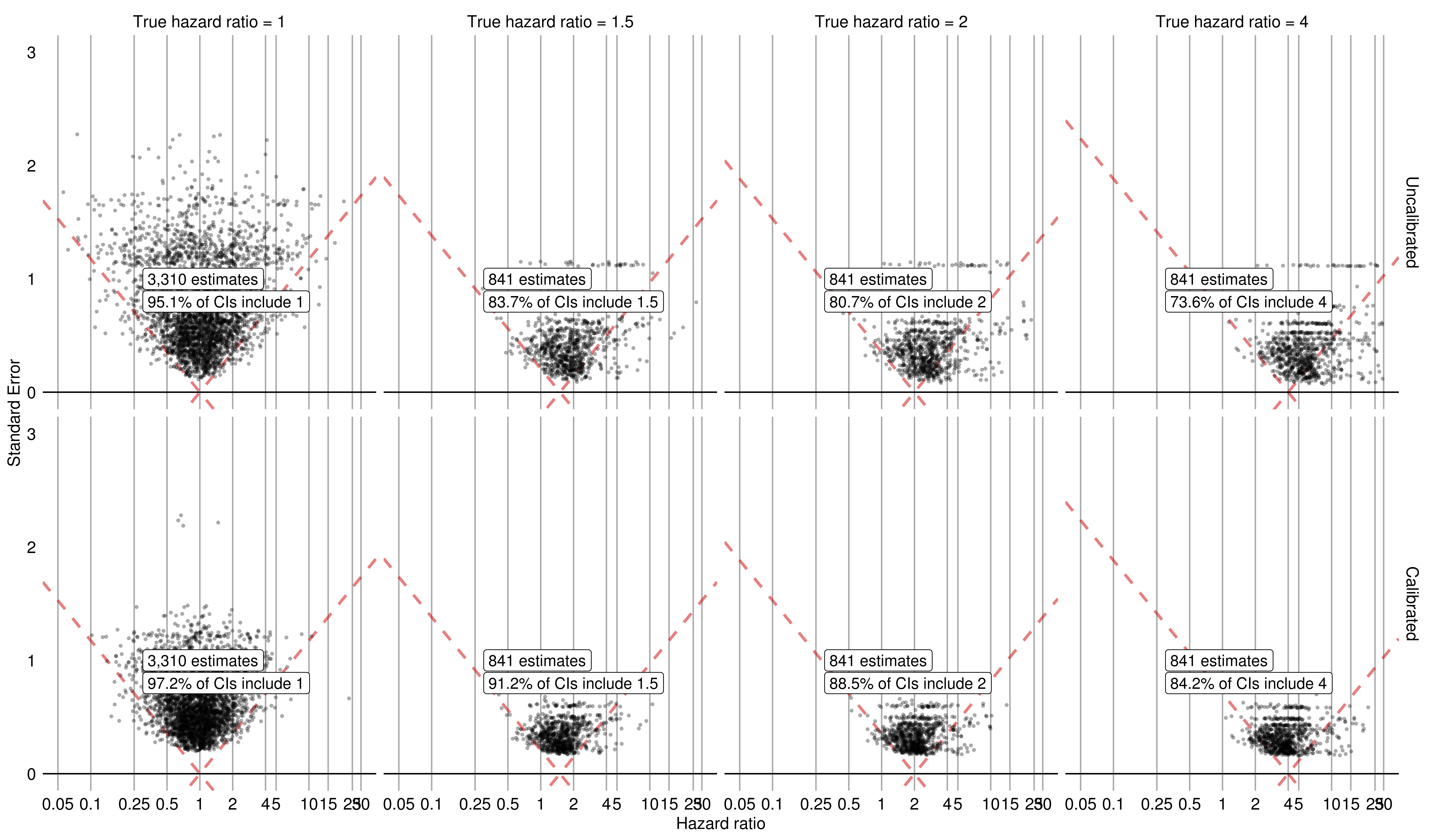
Figure 40: Evaluation of the effect estimation before (top) and after (bottom) calibration using the IMSG database in the hypertension data set. The linear model of bias was used and training was performed on both negative and positive controls.

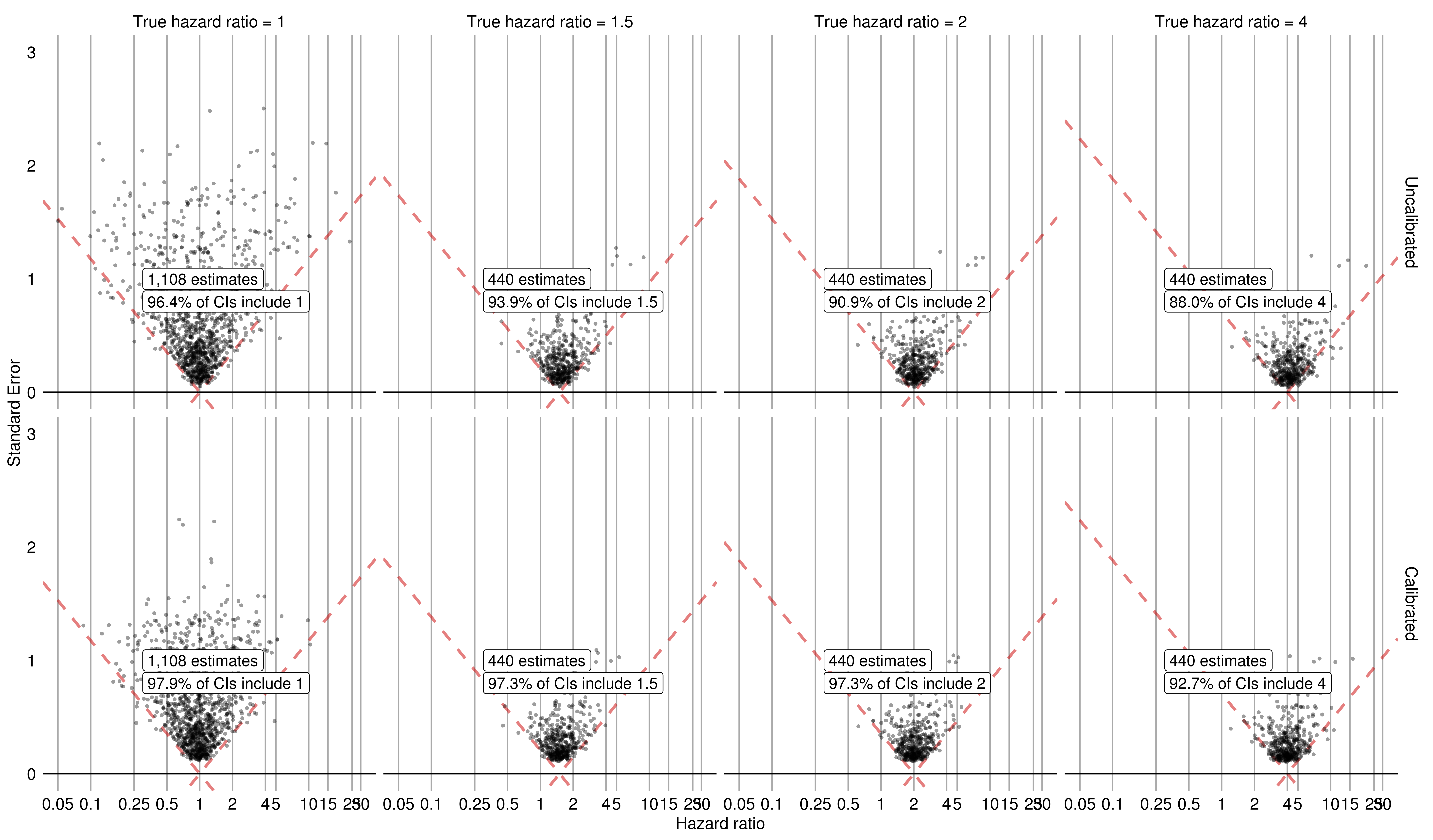
Figure 42: Evaluation of the effect estimation before (top) and after (bottom) calibration using the NHIS NSC database in the hypertension data set. The linear model of bias was used and training was performed on both negative and positive controls.

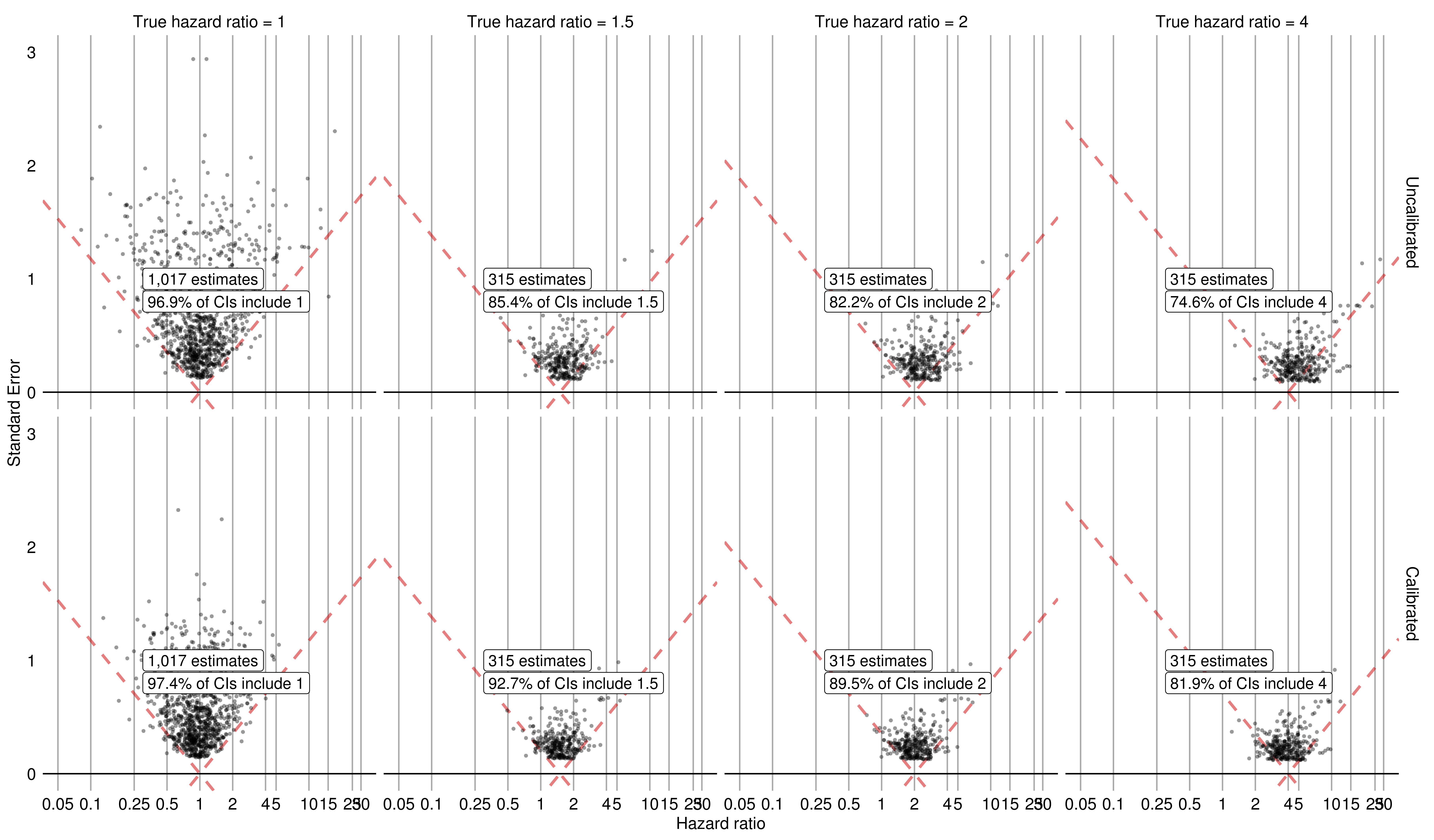
Figure 43: Evaluation of the effect estimation before (top) and after (bottom) calibration using the CUMC database in the hypertension data set. The linear model of bias was used and training was performed on both negative and positive controls.

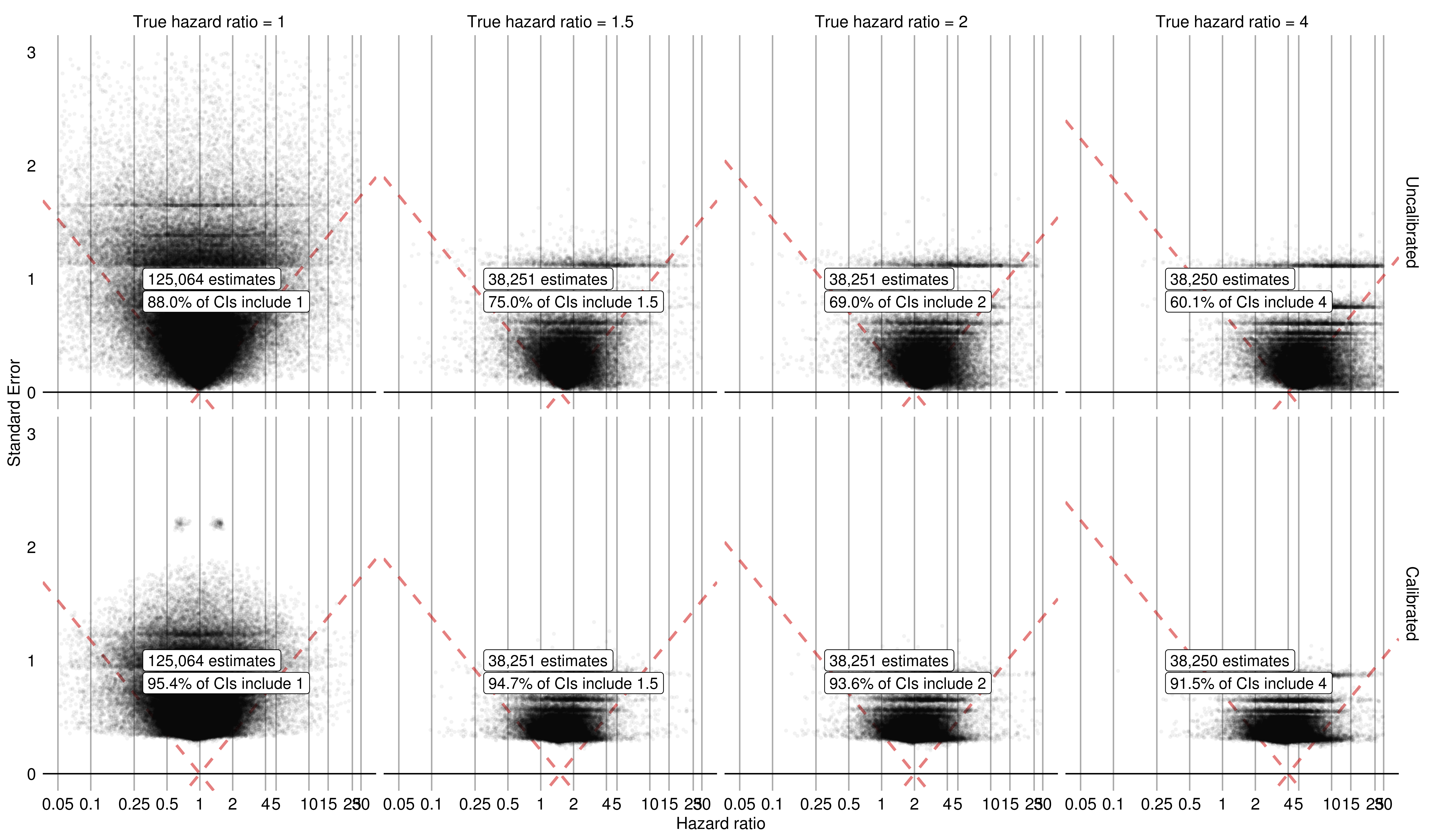
Figure 44: Evaluation of the effect estimation before (top) and after (bottom) calibration using the Panther database in the hypertension data set. The linear model of bias was used and training was performed on both negative and positive controls.

We conclude with the results of the linear model of the true bias. Figures 36, 37, 38, 39, 40, 41, 42, 43, and 44 report effect size estimates for all negative and positive controls across the nine databases as well as the percentage of posterior intervals containing the true effect size. The number of effect sizes that were tested are reported on the figures. The performance of these databases is similar to the constant model of bias: 1) For Optum, CCAE, MDCD, MDCR, and Panther, the calibrated procedure results in posterior intervals that are closer to 95% than the uncalibrated procedure, 2) For the CUMC, JMDC, and IMSG databases, for the hazard ratio of one, the uncalibrated procedure performed slightly better than the calibrated procedure, and for the other hazard ratios, the calibrated procedure performed better than the uncalibrated procedure, and 3) For the NHIS NSC database, the uncalibrated procedure performed slightly better for the hazard ratio of 1 and 1.5, and the calibrated procedure performed better for the hazard ratio of 2 and 4.

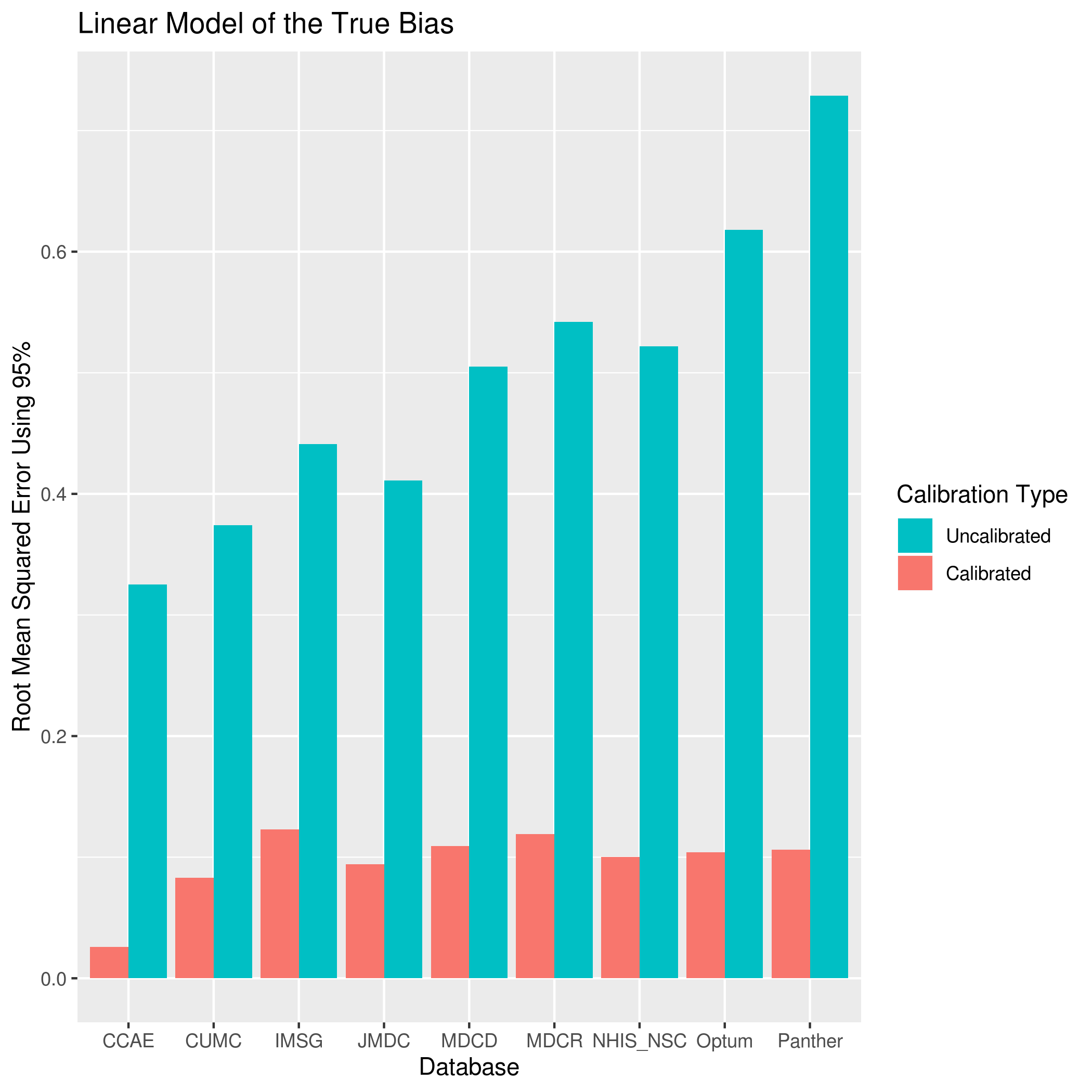
Figure 47: Root mean squared error of all effects before (uncalibrated) and after (calibrated) calibration for each of the nine databases in the hypertension data set. The linear model of bias was used and training was performed on both negative and positive controls.

For all nine databases, the calibrated procedure results in posterior intervals that are closer to 95% than the uncalibrated procedure. Figure 47 shows the RMSE calculated for each database. The uncalibrated procedure has higher error overall than the calibrated procedure, when considering all hazard ratios combined. There appears to be more error overall when using the linear model of the true bias compared to the constant model of the true bias.

The coverage for the calibrated and uncalibrated methods using the hypertension data set is displayed in Table 3.

4 Discussion

In the context of two large-scale clinical studies, we have shown that calibrating posterior intervals restores interval coverage to near-nominal levels. This enables appropriate interpretation for decision making. Our results are similar to those of ⁶, but our Bayesian formulation provides a framework for further extension. For example, we can develop models that explicitly incorporate the biases and variance implicit in choice of database or in choice of analytic methods. Future work will take advantage of the Bayesian paradigm to enable Bayesian meta-analysis and, to account for model uncertainty, Bayesian model averaging. We note that inclusion of synthetic positive controls impacted the results minimally. This may point to adopting a simpler approach of using only negative controls. Because they are simulated based on the negative controls, they do not add new information to the model, and further study of their benefit is warranted.

Our main assumptions are similar to those of ⁶. We require that our negative controls are truly negative so that their effect sizes are zero. Our method is therefore dependent upon our process for generating negative controls, which generally entails considering exposure-outcome pairs to be negative when both the exposure and the outcome are well-studied but lack evidence that the exposure causes the outcome in scientific literature, structured product labels, or spontaneous adverse event reports. Lack of evidence of an effect is not the same as lack of an effect, but⁶ demonstrated the validity of this approach to negative controls (see its Appendix).

We also require that our controls are in some sense exchangeable with the intervention-outcome pairs of interest. We emphasize here that the bias need not be identical, but instead that the variety of types of confounding that exists among the controls is such that the confounding that affects the hypothesis of interest could have been drawn from a hypothetical distribution of confounding types seen in the controls. We do not require the controls to have exactly the same magnitude and structure of confounding as the outcome of interest as other proposed approaches do. ^{2, 10} For this study, we used the normal distribution to model the bias. Other distributions can be considered, such a $t$-distribution, or a Bayesian nonparametric approach.

In summary, our Bayesian approach produced similar results to that of ⁶ and provide a diagnostic to detect unmeasured confounding as well as a means to restore proper interval coverage at the expense of generally wider confidence intervals. Our approach is amenable to extension to accommodate other sources of systematic error such as differences among databases and differences among analytic methods.

Data Accessibility

The data used in this article are freely available. Please contact the corresponding author for more information on how to obtain the data.

Financial disclosure

None reported.

Conflict of interest

The authors declare no potential conflict of interests.

Appendix A Additional Figures for the Depression Data Set

A.1 Depression Data Set

Figure 16: Root mean squared error of all effects after stratification on the propensity scores before (uncalibrated) and after (calibrated) calibration for each of the databases in the depression data set. The constant model of bias was used and training was performed on only negative controls.

			Effect Size
			1	1.5	2	4
Training Type	Database	Calibration Type	Coverage	Coverage	Coverage	Coverage
Constant	CCAE	Calibrated	$0.945$	$0.943$	$0.939$	$0.932$
		Uncalibrated	$0.826$	$0.759$	$0.743$	$0.703$
	MDCD	Calibrated	$0.950$	$0.937$	$0.929$	$0.932$
		Uncalibrated	$0.907$	$0.822$	$0.809$	$0.768$
	MDCR	Calibrated	$0.950$	$0.930$	$0.930$	$0.913$
		Uncalibrated	$0.902$	$0.818$	$0.813$	$0.760$
	Optum	Calibrated	$0.947$	$0.938$	$0.938$	$0.927$
		Uncalibrated	$0.852$	$0.793$	$0.768$	$0.721$
Linear	CCAE	Calibrated	$0.945$	$0.937$	$0.936$	$0.927$
		Uncalibrated	$0.826$	$0.759$	$0.743$	$0.703$
	MDCD	Calibrated	$0.955$	$0.932$	$0.932$	$0.931$
		Uncalibrated	$0.907$	$0.822$	$0.809$	$0.768$
	MDCR	Calibrated	$0.949$	$0.921$	$0.919$	$0.902$
		Uncalibrated	$0.902$	$0.818$	$0.813$	$0.760$
	Optum	Calibrated	$0.946$	$0.937$	$0.933$	$0.920$
		Uncalibrated	$0.852$	$0.793$	$0.768$	$0.721$
Train on Only Negative Controls	CCAE	Calibrated	$0.943$	$0.939$	$0.937$	$0.925$
		Uncalibrated	$0.826$	$0.759$	$0.743$	$0.703$
	MDCD	Calibrated	$0.950$	$0.936$	$0.928$	$0.928$
		Uncalibrated	$0.907$	$0.822$	$0.809$	$0.768$
	MDCR	Calibrated	$0.943$	$0.914$	$0.913$	$0.897$
		Uncalibrated	$0.902$	$0.818$	$0.813$	$0.760$
	Optum	Calibrated	$0.942$	$0.931$	$0.931$	$0.919$
		Uncalibrated	$0.852$	$0.793$	$0.768$	$0.721$

Table 2: Coverage for the calibrated and uncalibrated procedures on the depression data set.

Appendix B Additional Figures for the Hypertension Data Set

B.1 Hypertension Data Set

Figure 28: Evaluation of the effect estimation before (top) and after (bottom) calibration using the CCAE database in the hypertension data set. The constant model of bias was used and training was performed on only negative controls.

Figure 32: Evaluation of the effect estimation before (top) and after (bottom) calibration using the JMDC database in the hypertension data set. The constant model of bias was used and training was performed on only negative controls.

Figure 41: Evaluation of the effect estimation before (top) and after (bottom) calibration using the JMDC database in the hypertension data set. The linear model of bias was used and training was performed on both negative and positive controls.

			Effect Size
			1	1.5	2	4
Training Type	Database	Calibration Type	Coverage	Coverage	Coverage	Coverage
Constant	CCAE	Calibrated	$0.953$	$0.951$	$0.946$	$0.935$
		Uncalibrated	$0.876$	$0.802$	$0.770$	$0.702$
	CUMC	Calibrated	$0.977$	$0.956$	$0.956$	$0.911$
		Uncalibrated	$0.969$	$0.854$	$0.822$	$0.746$
	IMSG	Calibrated	$0.978$	$0.946$	$0.935$	$0.916$
		Uncalibrated	$0.951$	$0.837$	$0.807$	$0.736$
	JMDC	Calibrated	$0.967$	$0.953$	$0.953$	$0.938$
		Uncalibrated	$0.955$	$0.935$	$0.920$	$0.873$
	MDCD	Calibrated	$0.955$	$0.943$	$0.937$	$0.926$
		Uncalibrated	$0.890$	$0.805$	$0.771$	$0.719$
	MDCR	Calibrated	$0.964$	$0.955$	$0.946$	$0.924$
		Uncalibrated	$0.924$	$0.865$	$0.844$	$0.770$
	NHIS_NSC	Calibrated	$0.972$	$0.975$	$0.970$	$0.936$
		Uncalibrated	$0.964$	$0.939$	$0.909$	$0.880$
	Optum	Calibrated	$0.944$	$0.947$	$0.941$	$0.926$
		Uncalibrated	$0.859$	$0.783$	$0.748$	$0.678$
	Panther	Calibrated	$0.954$	$0.960$	$0.948$	$0.923$
		Uncalibrated	$0.880$	$0.750$	$0.690$	$0.601$
Linear	CCAE	Calibrated	$0.952$	$0.942$	$0.935$	$0.920$
		Uncalibrated	$0.876$	$0.802$	$0.770$	$0.702$
	CUMC	Calibrated	$0.974$	$0.927$	$0.895$	$0.819$
		Uncalibrated	$0.969$	$0.854$	$0.822$	$0.746$
	IMSG	Calibrated	$0.972$	$0.912$	$0.885$	$0.842$
		Uncalibrated	$0.951$	$0.837$	$0.807$	$0.736$
	JMDC	Calibrated	$0.967$	$0.982$	$0.961$	$0.938$
		Uncalibrated	$0.955$	$0.935$	$0.920$	$0.873$
	MDCD	Calibrated	$0.951$	$0.924$	$0.917$	$0.898$
		Uncalibrated	$0.890$	$0.805$	$0.771$	$0.719$
	MDCR	Calibrated	$0.957$	$0.933$	$0.922$	$0.892$
		Uncalibrated	$0.924$	$0.865$	$0.844$	$0.770$
	NHIS_NSC	Calibrated	$0.979$	$0.973$	$0.973$	$0.927$
		Uncalibrated	$0.964$	$0.939$	$0.909$	$0.880$
	Optum	Calibrated	$0.946$	$0.942$	$0.935$	$0.919$
		Uncalibrated	$0.859$	$0.783$	$0.748$	$0.678$
	Panther	Calibrated	$0.954$	$0.947$	$0.936$	$0.915$
		Uncalibrated	$0.880$	$0.750$	$0.690$	$0.601$
Train on Only Negative Controls	CCAE	Calibrated	$0.945$	$0.939$	$0.930$	$0.915$
		Uncalibrated	$0.876$	$0.802$	$0.770$	$0.702$
	CUMC	Calibrated	$0.973$	$0.895$	$0.857$	$0.784$
		Uncalibrated	$0.969$	$0.854$	$0.822$	$0.746$
	IMSG	Calibrated	$0.962$	$0.889$	$0.853$	$0.797$
		Uncalibrated	$0.951$	$0.837$	$0.807$	$0.736$
	JMDC	Calibrated	$0.964$	$0.956$	$0.956$	$0.935$
		Uncalibrated	$0.955$	$0.935$	$0.920$	$0.873$
	MDCD	Calibrated	$0.940$	$0.915$	$0.906$	$0.886$
		Uncalibrated	$0.890$	$0.805$	$0.771$	$0.719$
	MDCR	Calibrated	$0.951$	$0.930$	$0.920$	$0.881$
		Uncalibrated	$0.924$	$0.865$	$0.844$	$0.770$
	NHIS_NSC	Calibrated	$0.971$	$0.968$	$0.966$	$0.936$
		Uncalibrated	$0.964$	$0.939$	$0.909$	$0.880$
	Optum	Calibrated	$0.940$	$0.939$	$0.931$	$0.914$
		Uncalibrated	$0.859$	$0.783$	$0.748$	$0.678$
	Panther	Calibrated	$0.949$	$0.935$	$0.911$	$0.869$
		Uncalibrated	$0.880$	$0.750$	$0.690$	$0.601$

Table 3: Table displaying coverage for the calibrated and uncalibrated procedures on the hypertension data set.

References

- 1 Lipsitch M, Tchetgen Tchetgen E, Cohen T. Negative Controls: A Tool for Detecting Confounding and Bias in Observational Studies. Epidemiology 2010; 21(3): 383–388. doi: 10.1097/EDE.0b013e3181d61eeb
- 2 Tchetgen Tchetgen E. The Control Outcome Calibration Approach for Causal Inference With Unobserved Confounding. American Journal of Epidemiology 2014; 179(5): 633–640. doi: 10.1093/aje/kwt303
- 3 Dusetzina SB, Brookhart MA, Maciejewski ML. Control Outcomes and Exposures for Improving Internal Validity of Nonrandomized Studies. Health Services Research 2015; 50(5): 1432–1451. doi: 10.1111/1475-6773.12279
- 4 Arnold BF, Ercumen A, Benjamin-Chung J, Colford JM. Brief Report: Negative Controls to Detect Selection Bias and Measurement Bias in Epidemiologic Studies. Epidemiology 2016; 27(5): 637–641. doi: 10.1097/EDE.0000000000000504
- 5 Desai JR, Hyde CL, Kabadi S, et al. Utilization of Positive and Negative Controls to Examine Comorbid Associations in Observational Database Studies:. Medical Care 2017; 55(3): 244–251. doi: 10.1097/MLR.0000000000000640
- 6 Schuemie MJ, Hripcsak G, Ryan PB, Madigan D, Suchard MA. Empirical confidence interval calibration for population-level effect estimation studies in observational healthcare data. Proceedings of the National Academy of Sciences 2018; 115(11): 2571–2577. doi: 10.1073/pnas.1708282114
- 7 Schuemie MJ, Ryan PB, Hripcsak G, Madigan D, Suchard MA. Improving reproducibility by using high-throughput observational studies with empirical calibration. Philosophical Transactions of the Royal Society A: Mathematical, Physical and Engineering Sciences 2018; 376(2128): 20170356. doi: 10.1098/rsta.2017.0356
- 8 Schuemie MJ, Ryan PB, DuMouchel W, Suchard MA, Madigan D. Interpreting observational studies: why empirical calibration is needed to correct p -values. Statistics in Medicine 2014; 33(2): 209–218. doi: 10.1002/sim.5925
- 9 Suchard MA, Schuemie MJ, Krumholz HM, et al. Comprehensive comparative effectiveness and safety of first-line antihypertensive drug classes: a systematic, multinational, large-scale analysis. The Lancet 2019; 394(10211): 1816–1826. doi: 10.1016/S0140-6736(19)32317-7
- 10 Flanders WD, Strickland MJ, Klein M. A New Method for Partial Correction of Residual Confounding in Time-Series and Other Observational Studies. American Journal of Epidemiology 2017; 185(10): 941–949. doi: 10.1093/aje/kwx013