Estimating Basis Functions in Massive Fields under the Spatial Mixed Effects Model

Abstract

Spatial prediction is commonly achieved under the assumption of a Gaussian random field (GRF) by obtaining maximum likelihood estimates of parameters, and then using the kriging equations to arrive at predicted values. For massive datasets, fixed rank kriging using the Expectation-Maximization (EM) algorithm for estimation has been proposed as an alternative to the usual but computationally prohibitive kriging method. The method reduces computation cost of estimation by redefining the spatial process as a linear combination of basis functions and spatial random effects. A disadvantage of this method is that it imposes constraints on the relationship between the observed locations and the knots. We develop an alternative method that utilizes the Spatial Mixed Effects (SME) model, but allows for additional flexibility by estimating the range of the spatial dependence between the observations and the knots via an Alternating Expectation Conditional Maximization (AECM) algorithm. Experiments show that our methodology improves estimation without sacrificing prediction accuracy while also minimizing the additional computational burden of extra parameter estimation. The methodology is applied to a temperature data set archived by the United States National Climate Data Center, with improved results over previous methodology.

I Introduction

In geostatistics, spatial estimation and prediction are often the primary focus. It is assumed that nearby observations tend to be more similar than those far apart. Since observations are spatially correlated, modeling the dependence structure can provide insight into the spatial phenomena and can be used to improve prediction. To formalize ideas, let $\boldsymbol{s}=\{\boldsymbol{s}_{1},\boldsymbol{s}_{2},\ldots,\boldsymbol{s}_{n}\}\in\mathcal{D}$ represent all observed locations and let $\boldsymbol{s}_{0}=\{\boldsymbol{s}_{01},\boldsymbol{s}_{02},\ldots,\boldsymbol{s}_{0N}\}\in\mathcal{D}$ represent the desired locations, where $\mathcal{D}$ is a spatial domain. The two sets of locations $\boldsymbol{s}$ and $\boldsymbol{s}_{0}$ may (or may not) have common elements. Let $y(\cdot)$ be the random process defined on $\mathcal{D}$. Generally, $y(\cdot)$ is characterized as a linear combination of three main components: a mean structure $\mu(\cdot)$, a zero-mean spatial process $f(\cdot)$, and a zero-mean measurement error process $\epsilon(\cdot)$, i.e.

$$\boldsymbol{y}(\boldsymbol{s})=\boldsymbol{\mu}(\boldsymbol{s})+\boldsymbol{f}(\boldsymbol{s})+\boldsymbol{\epsilon}(\boldsymbol{s}),$$ (1)

where $f(\cdot)$ and $\epsilon(\cdot)$ are typically assumed to be Gaussian processes. Any likelihood-based estimation procedure involves evaluating the log-likelihood

$$\begin{split}\ell(\boldsymbol{\theta})\propto&-\frac{1}{2}[\boldsymbol{y}(\boldsymbol{s})-\boldsymbol{\mu}(\boldsymbol{s})]^{\prime}\{\mbox{Cov}[\boldsymbol{y}(\boldsymbol{s}),\boldsymbol{y}(\boldsymbol{s})]\}^{-1}[\boldsymbol{y}(\boldsymbol{s})-\boldsymbol{\mu}(\boldsymbol{s})]\\ &-\frac{1}{2}\log\{|\mbox{Cov}[\boldsymbol{y}(\boldsymbol{s}),\boldsymbol{y}(\boldsymbol{s})]|\}.\end{split}$$ (2)

Under squared error loss, the Best Linear Unbiased Predictions (BLUP) – equivalently, [1]’s kriged estimate – of $y(\cdot)$ at the desired locations $\boldsymbol{s}_{0}$ can be computed using the first two moments of $y(\cdot)$ (see e.g. [2]) as:

$$\begin{split}\hat{\boldsymbol{y}}(\boldsymbol{s}_{0})=&\mbox{E}(\boldsymbol{y}(\boldsymbol{s}_{0}))+\mbox{Cov}[\boldsymbol{y}(\boldsymbol{s}_{0}),\boldsymbol{y}(\boldsymbol{s})]\{\mbox{Cov}[\boldsymbol{y}(\boldsymbol{s}),\boldsymbol{y}(\boldsymbol{s})]\}^{-1}\\ &[\boldsymbol{y}(\boldsymbol{s}_{0})-\mbox{E}(\boldsymbol{y}(\boldsymbol{s}_{0}))].\end{split}$$ (3)

Both (2) and (3) involve inverting a covariance matrix of order $n\times n$ which is an $O(n^{3})$ operation and thus computationally impractical for massive datasets in terms of both CPU time and memory. The need for such predictions in massive spatial datasets however exist, for example in satellite data where observations are recorded across the entire globe or more localized spatial domains in which the fine resolution results in a large $n$. In such scenarios, it is computationally infeasible to obtain the kriged estimates provided by (3) even on modern computing hardware.

The development of efficient kriging methods has received substantial attention in the literature. Much of this development has focused either on approximating the kriging equations of (3) [3, 4, 5, 6, 7, 8, 9, 10, 11, 12, 13, 14] or on defining a covariance structure that allows for exact kriging, regardless of the size of the data [15, 16, 17, 18, 19, 20, 21, 22, 23]. In this paper, we develop methodology that is capable of modeling severe nonstationarity while providing useful parameter interpretation in an efficient manner and without loss of prediction accuracy. Our underlying framework uses the “Spatial Mixed Effects” (SME) model defined by [18] to obtain parameter estimates and spatial predictions, as it provides a good compromise between flexibility in the covariance structure and computational efficiency. See [24] for a more detailed comparison of some of the different approaches.

While [20] allow for parameter estimation for nonstationary random fields, this methodology assumes the dependence structure between observations is the same as between observations and “knots”, a lower-dimensional subspace. However, we desire a more flexible model that allows for cross-regional dependence, which can be achieved by the SME model. In addition, the computational cost is prohibitive for massive data, as pointed out by [24]. Although [21] and [22] are equally as efficient, again, the flexibility of the assumed covariance structure is more restrictive.

Use of so-called low-rank approaches, such as fixed rank kriging through the SME model, have been called into question by [25]. The author illustrates, through both theory and simulation, how prediction and model fit can actually be improved by assuming independent spatial block and using the corresponding methodology, such as [3, 11]. However, in this paper, our focus is on estimation and prediction of spatial models that may possess significant regional dependence, where the assumption of independent blocks is clearly inappropriate. Therefore, we now discuss the SME model in some detail.

I-A Spatial Mixed Effects Model

Within the framework (1), the SME model uses a linear combination of fixed basis functions and a set of locations with reduced cardinality ($m<n$) known as knots to define the spatial process at the original set $\boldsymbol{s}$. A fine-scale variation process $\delta(\cdot)$ is also added to the model. Let $\eta(\cdot)$ represent a Gaussian random effect, define $\boldsymbol{u}=\{\boldsymbol{u}_{1},\ldots,\boldsymbol{u}_{m}\}$ to be the knots, and let $S_{k}(\cdot)$ define the basis function corresponding to the $k$th knot. Under the SME model, the usual spatial process $f(\cdot)$ is then replaced by the linear combination of basis functions and the fine-scale variation process. With a linear mean structure, the model for a single observation $\boldsymbol{s}_{i}$ is

$$y(\boldsymbol{s}_{i})=\boldsymbol{x}(\boldsymbol{s}_{i})^{\prime}\boldsymbol{\beta}+\sum_{k=1}^{m}S_{k}(\boldsymbol{s}_{i})\eta(\boldsymbol{u}_{k})+\delta(\boldsymbol{s}_{i})+\epsilon(\boldsymbol{s}_{i}),$$ (4)

where $\boldsymbol{x}(\cdot)=[x_{1}(\cdot),\ldots,x_{p}(\cdot)]^{\prime}$ is a vector of known covariates with (unknown) coefficients $\boldsymbol{\beta}=(\beta_{1},\ldots,\beta_{p})^{\prime}$. Also, let $\boldsymbol{\eta}(\boldsymbol{u})\sim N(\boldsymbol{0},\boldsymbol{K})$, $\boldsymbol{\delta}(\boldsymbol{s})\sim N(\boldsymbol{0},\sigma_{\delta}^{2}\boldsymbol{V}_{\delta})$, and $\boldsymbol{\epsilon}(\boldsymbol{s})\sim N(\boldsymbol{0},\sigma_{\epsilon}^{2}\boldsymbol{V}_{\epsilon})$ be mutually independent with $\boldsymbol{V}_{\delta}$ and $\boldsymbol{V}_{\epsilon}$ known diagonal matrices with entries corresponding to the fine-scale and measurement error variances, respectively. These diagonal elements are realizations of known functions $v_{\delta}(\cdot)$ and $v_{\epsilon}(\cdot)$.

Define the dispersion matrix of $y(\cdot)$ by $\boldsymbol{\Sigma}=\boldsymbol{S}\boldsymbol{K}\boldsymbol{S}^{\prime}+\sigma_{\delta}^{2}\boldsymbol{V}_{\delta}+\sigma_{\epsilon}^{2}\boldsymbol{V}_{\epsilon}$ with $\boldsymbol{S}$ denoting the full $n\times m$-matrix of basis functions with $k$th column given by $\boldsymbol{S}_{k}(\boldsymbol{s})$. Defining $\boldsymbol{X}$ as the design matrix for the mean structure, the log-likelihood for $y(\cdot)$ in simplified matrix notation is then the usual

$$\ell(\boldsymbol{K},\sigma_{\delta}^{2},\sigma_{\epsilon}^{2},\boldsymbol{\beta};\boldsymbol{y}) \propto -\frac{1}{2}(\boldsymbol{y}-\boldsymbol{X}\boldsymbol{\beta})^{\prime}\boldsymbol{\Sigma}^{-1}(\boldsymbol{y}-\boldsymbol{X}\boldsymbol{\beta})$$ (5)

$$-\frac{1}{2}\log(|\boldsymbol{\Sigma}|).$$

Spatial predictions require the covariance between the set of observations and the desired locations, $\mbox{Cov}[\boldsymbol{y}(\boldsymbol{s}_{0}),\boldsymbol{y}(\boldsymbol{s})]$. Let $\boldsymbol{A}=[\boldsymbol{S}_{1}(\boldsymbol{s}_{0}),\ldots,\boldsymbol{S}_{m}(\boldsymbol{s}_{0})]^{\prime}$ be the $N\times m$ matrix of basis functions relating the knots to the desired locations and define $\boldsymbol{I}_{s}$ as an $N\times n$ matrix with entries equal to $I_{s}(i,j)=I[\boldsymbol{s}_{0i}=\boldsymbol{s}_{j}]$. We then define the covariance,

$$\boldsymbol{C}(\boldsymbol{s}_{0})=\mbox{Cov}[\boldsymbol{y}(\boldsymbol{s}_{0}),\boldsymbol{y}(\boldsymbol{s})]=\boldsymbol{A}\boldsymbol{K}\boldsymbol{S}^{\prime}+\sigma_{\delta}^{2}v_{\delta}(\boldsymbol{s}_{0})\boldsymbol{I}_{s}$$ (6)

and the kriging estimates – see Section 3.4.5 of [2] – as

$$\hat{\boldsymbol{y}}(\boldsymbol{s}_{0})=\boldsymbol{X}(\boldsymbol{s}_{0})\hat{\boldsymbol{\beta}}+\boldsymbol{C}(\boldsymbol{s}_{0})\boldsymbol{\Sigma}^{-1}(\boldsymbol{y}-\boldsymbol{X}\hat{\boldsymbol{\beta}})$$ (7)

where $\hat{\boldsymbol{\beta}}=(\boldsymbol{X}^{\prime}\boldsymbol{\Sigma}^{-1}\boldsymbol{X})^{-1}\boldsymbol{X}^{\prime}\boldsymbol{\Sigma}^{-1}\boldsymbol{y}$. The kriging standard error (KSE) is given by $\hat{\boldsymbol{\sigma}}_{k}(\boldsymbol{s}_{0})=\{\boldsymbol{A}\boldsymbol{K}\boldsymbol{A}^{\prime}+\sigma_{\delta}^{2}\boldsymbol{V}_{\delta}(\boldsymbol{s}_{0})-\boldsymbol{C}(\boldsymbol{s}_{0})\boldsymbol{\Sigma}^{-1}\boldsymbol{C}(\boldsymbol{s}_{0})^{\prime}+[\boldsymbol{X}(\boldsymbol{s}_{0})-\boldsymbol{X}^{\prime}\boldsymbol{\Sigma}^{-1}\boldsymbol{C}(\boldsymbol{s}_{0})^{\prime}]^{\prime}\linebreak(\boldsymbol{X}^{\prime}\boldsymbol{\Sigma}^{-1}\boldsymbol{X})^{-1}[\boldsymbol{X}(\boldsymbol{s}_{0})-\boldsymbol{X}^{\prime}\boldsymbol{\Sigma}^{-1}\boldsymbol{C}(\boldsymbol{s}_{0})^{\prime}]\}^{\frac{1}{2}}$ [18] where $\boldsymbol{V}_{\delta}(\boldsymbol{s}_{0})$ is diagonal matrix with diagonal entries given by the function $v_{\delta}(\cdot)$ evaluated at $\boldsymbol{s}_{0}$. By defining $\boldsymbol{D}=\sigma_{\delta}^{2}\boldsymbol{V}_{\delta}+\sigma_{\epsilon}^{2}\boldsymbol{V}_{\epsilon}$, the computational burden of matrix inversion is reduced using the identity

$$\boldsymbol{\Sigma}^{-1}=\boldsymbol{D}^{-1}-\boldsymbol{D}^{-1}\boldsymbol{S}[\boldsymbol{K}^{-1}+\boldsymbol{S}^{\prime}\boldsymbol{D}^{-1}\boldsymbol{S}]^{-1}S^{\prime}\boldsymbol{D}^{-1},$$ (8)

which follows from the Sherman-Morrison-Woodbury formula [26]. Note that the inversion of the $n\times n$ matrix $\boldsymbol{\Sigma}^{-1}$ is replaced by that of two (smaller) $m\times m$ matrices and the diagonal matrix, $\boldsymbol{D}$. [18] recommended the Method of Moments estimator for the parameters in order to guarantee positive definiteness of $\hat{\boldsymbol{K}}$, the estimate of $\boldsymbol{K}$.

An alternative approach [27] obtained maximum likelihood estimates (MLEs) using the Expectation-Maximization (EM) algorithm [28] with $\boldsymbol{y}$ treated as the observed data and $\boldsymbol{\eta}$ and $\boldsymbol{\epsilon}$ as the missing data. In the absence of independent information regarding the measurement error of the process, [29] provide a method of estimating $\sigma_{\epsilon}^{2}$ that involves extrapolating the semivariogram back to the origin. Therefore, [27] assume that $\sigma_{\epsilon}^{2}$ is known or can be obtained independently. We adopt the same approach in this paper. Starting from initial values, the variance parameter estimates are obtained upon updating

$$\boldsymbol{K}^{(t+1)} = \boldsymbol{K}^{(t)}-\boldsymbol{K}^{(t)}\boldsymbol{S}^{\prime}{\boldsymbol{\Sigma}^{(t)}}^{-1}\boldsymbol{S}\boldsymbol{K}^{(t)}$$

$$+ [\boldsymbol{K}^{(t)}\boldsymbol{S}^{\prime}{\boldsymbol{\Sigma}^{(t)}}^{-1}(\boldsymbol{y}-\boldsymbol{X}\hat{\boldsymbol{\beta}})]$$

$$[\boldsymbol{K}^{(t)}\boldsymbol{S}^{\prime}{\boldsymbol{\Sigma}^{(t)}}^{-1}(\boldsymbol{y}-\boldsymbol{X}\hat{\boldsymbol{\beta}})]^{\prime}$$

$$\sigma_{\delta}^{2(t+1)} = \sigma_{\delta}^{2(t)}+\frac{(\sigma_{\delta}^{2(t)})^{2}}{n}\mbox{tr}[{\boldsymbol{\Sigma}^{(t)}}^{-1}((\boldsymbol{y}-\boldsymbol{X}\hat{\boldsymbol{\beta}})$$

$$(\boldsymbol{y}-\boldsymbol{X}\hat{\boldsymbol{\beta}})^{\prime}{\boldsymbol{\Sigma}^{(t)}}^{-1}-\boldsymbol{I})\boldsymbol{V}_{\delta}],$$

from the $t$th to the $(t+1)$th iteration, and proceeding till convergence. The estimate of $\boldsymbol{\beta}$ denoted by $\hat{\boldsymbol{\beta}}$ is obtained using generalized least squares (GLS) as in (7).

This methodology assumes that the basis functions are fully specified smoothing functions. [18] and [27] use the local bisquare function. We provide further details in Section II-A but note that this function requires a tuning parameter, which the authors set at a constant 1.5 times the minimum distance between the inter-knot distance. In the context of spatial statistics, this tuning parameter has interpretation similar to the range parameter and so estimation provides insight into the rate of decay of spatial dependence. Further, inaccurate specification of this parameter has the potential to also result in poor prediction, therefore our methodology details an extension to the EM algorithm that allows for estimation of a “range” parameter within $\boldsymbol{S}$.

This paper is organized as follows. In Section 2 of this paper we propose a combination of concepts from the EM approach to fixed rank kriging (FRK) and the Alternating Expectation Conditional Maximization algorithm (AECM) [30, 31] that allows for computationally practical estimation of a continuous parameter within the basis functions, similar to the use of the ECM for spatio-temporal problems by [32]. Results of extensive simulation-based evaluations of our methodology in Section 3 show that estimation of the basis functions can improve prediction and is robust against certain model misspecification. Section 4 demonstrates the applicability of our methodology to predicting temperatures across the US. We conclude with some discussion and pointers to future work.

II Methodology

II-A Choice of Basis Functions

Fixed rank kriging and the proceeding EM estimation methodology recommend the use of multi-resolution basis functions in order to capture different scales of spatial variation. In particular, they use the local bisquare function which defines the basis function at the $l$th resolution as

$$S_{k(l)}(\boldsymbol{x})=\Psi\left(\frac{\|\boldsymbol{x}-\boldsymbol{u}_{k(l)}\|}{r_{l}}\right)\quad\forall\mbox{ }\boldsymbol{x}\in D,$$ (10)

where $\boldsymbol{u}_{k(l)}$ is a knot assigned to the $l$th resolution, with $l=\{1,\ldots,L\}$. $\Psi(d)$ is the local bisquare function defined as

$$\Psi(d)=\left\{\begin{array}[]{l l}\left(1-d^{2}\right)^{2}&\quad 0\leq d\leq 1\\ 0&\quad d>1\\ \end{array}\right.$$ (11)

where $r_{l}=b\hskip 2.84526pt\mbox{min}\{\|\boldsymbol{u}_{i(l)}-\boldsymbol{u}_{j(l)}\|:j\neq i,1\leq i,j\leq m\}$ and $b$ is some constant. We follow the recommendation and notation of these papers by defining our matrix of basis functions $\boldsymbol{S}$ by (10) and (11). This form is particularly useful in that (11) sets any value equal to zero where the distance between the location and the knot is greater than $r_{l}$, the “bandwidth”. This allows the opportunity to utilize matrix operations and algorithms (see e.g. [33]) that have been specifically designed to exploit sparsity. The distances are often defined in terms of the Euclidean norm, however this is not a necessary condition, as shown in our application to temperature data.

In practice, the number of knots used in prediction will be a function of the computational resources available and, consequently, may be considered to be known. From (10), it is clear that the remaining unknowns are the resolution $l$ and the bandwidth constant $b$. The optimal resolution is one of a finite, and generally small, set of positive integers. Given a finite set, estimation and prediction with varying resolutions remain easily parallelizable processes and so a model selection approach comparing performance of varying levels of resolution can be implemented. The domain of $b$ is $\mbox{I\!R}^{+}$, so a model selection approach would require a discretized domain. This approach can provide an estimate for $b$ that will produce reasonable predictions, however numerous estimation chains may be necessary and if the set of a priori selected possible values for $b$ does not encompass the true value, the estimate will be biased. Maintaining a model selection approach to determining the optimal resolution, $l$, we now direct our focus to improved estimation of $b$.

II-B Restricted Maximum Likelihood Estimation of Bandwidth

This section develops methodology for obtaining a restricted maximum likelihood (REML) estimate of $b$ along with those for $\boldsymbol{K}$ and $\sigma_{\delta}^{2}$. As noted by [34], an analytic solution to ML estimation of the parameters in the SME model does not appear to exist and direct numerical ML estimation is also challenging in that it requires maintaining a positive definite covariance matrix $\boldsymbol{K}$. For these reasons, the EM algorithm was used for parameter estimation.

When implementing the EM algorithm to estimate $b$, we wish to keep the advantageous structure of $\boldsymbol{S}$ intact. To avoid singularity issues during estimation, we also assume that $\sigma_{\epsilon}^{2}$ is known and that GLS is used to estimate $\boldsymbol{\beta}$, as before. Thus, we follow [27] and the remaining two random variables play the role of “missing values”: $\boldsymbol{\eta}$ and $\boldsymbol{\delta}$. Assuming independence of $\boldsymbol{\eta}\sim N(\boldsymbol{0},\boldsymbol{K})$ and $\boldsymbol{\delta}\sim N(\boldsymbol{0},\sigma_{\delta}^{2}\boldsymbol{V}_{\delta})$, we denote $\boldsymbol{\theta}^{[t]}=\{\boldsymbol{K}^{[t]},\sigma_{\delta}^{2[t]},b^{[t]}\}$ as the parameter values at the $t$th iteration. The analytical solution to the M-step of the EM algorithm then requires maximizing

$$\begin{split}Q(\boldsymbol{\theta};\boldsymbol{\theta}^{[t]})=&-\frac{1}{2}\{\log|\boldsymbol{K}|+\mbox{tr}(\boldsymbol{K}^{-1}E_{\boldsymbol{\theta}^{[t]}}[\boldsymbol{\eta}\boldsymbol{\eta}^{\prime}\mid\boldsymbol{y}])\\ &+\log(\sigma_{\delta}^{2n}|\boldsymbol{V}_{\delta}|)+\frac{1}{\sigma_{\delta}^{2}}\mbox{tr}(\boldsymbol{V}_{\delta}^{-1}E_{\boldsymbol{\theta}^{[t]}}[\boldsymbol{\delta}\boldsymbol{\delta}^{\prime}\mid\boldsymbol{y}])\\ &+\frac{1}{\sigma_{\epsilon}^{2}}\mbox{tr}(\boldsymbol{V}_{\epsilon}^{-1}[\boldsymbol{y}-\boldsymbol{X}\boldsymbol{\beta}-\boldsymbol{S}E_{\boldsymbol{\theta}^{[t]}}[\boldsymbol{\eta}\mid\boldsymbol{y}]\\ &-E_{\boldsymbol{\theta}^{[t]}}[\boldsymbol{\delta}\mid\boldsymbol{y}]][\boldsymbol{y}-\boldsymbol{X}\boldsymbol{\beta}-\boldsymbol{S}E_{\boldsymbol{\theta}^{[t]}}[\boldsymbol{\eta}\mid\boldsymbol{y}]\\ &-E_{\boldsymbol{\theta}^{[t]}}[\boldsymbol{\delta}\mid\boldsymbol{y}]]^{\prime})\}\end{split}$$ (12)

Maximizing (12) involves taking partial derivatives with respect to each parameter. For $\boldsymbol{K}$ and $\sigma_{\delta}^{2}$, this is fairly straightforward as these parameters appear separately within the summation. Thus, the resulting updating scheme includes the equations found in (I-A). Partial differentiation with respect to $b$, however, involves taking the derivative of a quartic term nested within the matrix of multi-resolution basis functions. An analytic solution does not exist, and the usual EM algorithm does not appear to show much promise. So we develop an AECM algorithm to estimate $b$.

II-C Estimating Bandwidth through AECM

In order to exploit the analytical iterative updating scheme for $\boldsymbol{K}$ and $\sigma_{\delta}^{2}$, we partition the parameters as $\boldsymbol{\theta}_{1}=\{\boldsymbol{K},\sigma_{\delta}^{2}\}$ and $\theta_{2}=\{b\}$. The CM-step of the AECM algorithm alternates between maximizing the likelihood function (12) with respect to $\boldsymbol{\theta}_{1}$ (keeping $\theta_{2}$ fixed at its current value) and $\theta_{2}$ (by holding $\boldsymbol{\theta}_{1}$ fixed at its current value). $\boldsymbol{\theta}_{1}$ is, therefore, updated by (I-A) as before. An estimate for $\theta_{2}$, however, cannot be calculated analytically nor numerically, so in lieu of maximizing (12), we maximize the restricted log-likelihood function given by

$$\begin{split}\ell(\boldsymbol{K},\sigma_{\delta}^{2},b;\boldsymbol{y},\sigma_{\epsilon}^{2})\propto&-\frac{1}{2}(\boldsymbol{y}-\boldsymbol{X}\hat{\boldsymbol{\beta}})^{\prime}\boldsymbol{\Sigma}^{-1}(\boldsymbol{y}-\boldsymbol{X}\hat{\boldsymbol{\beta}})\\ &-\frac{1}{2}\log(|\boldsymbol{\Sigma}|)-\frac{1}{2}\log(|\boldsymbol{X}^{\prime}\boldsymbol{\Sigma}^{-1}\boldsymbol{X}|).\end{split}$$ (13)

When restricted to be a function of $\theta_{2}$, (13) involves a covariance matrix which is in a form that allows for the use of dimension reduction equalities in the matrix calculations. As noted in [18], the Sherman-Morrison-Woodbury formula can be used to obtain a computationally efficient form of $\boldsymbol{\Sigma}^{-1}$. To avoid the burdensome computation of the determinant, we also invoke Sylvester’s determinant theorem [35, 18], which is an analogue to the Sherman-Morrison-Woodbury formula. Let $\boldsymbol{X}$ be an invertible $n\times n$ matrix, $\boldsymbol{A}$ an $n\times m$ matrix, $\boldsymbol{B}$ an $m\times n$ matrix, and $\boldsymbol{I}_{m}$ is the $m\times m$ identity matrix then $\det(\boldsymbol{X}+\boldsymbol{A}\boldsymbol{B})=\det(\boldsymbol{X})\det(\boldsymbol{I}_{m}+\boldsymbol{B}\boldsymbol{X}^{-1}\boldsymbol{A})$. Let $\boldsymbol{C}$ be the Cholesky decomposition of $\boldsymbol{K}$ ($\boldsymbol{K}=\boldsymbol{C}\boldsymbol{C}^{\prime}$). This theorem along with the fact that $\boldsymbol{K}$ is positive definite and some algebra takes us to the reduction

$$\det(\boldsymbol{D}+\boldsymbol{S}\boldsymbol{K}\boldsymbol{S}^{\prime})=\det(\boldsymbol{D})\det(\boldsymbol{C})^{2}\det(\boldsymbol{K}^{-1}+\boldsymbol{S}^{\prime}\boldsymbol{D}^{-1}\boldsymbol{S})$$ (14)

which provides us with the advantage that it requires computing an inverse of an $m\times m$ matrix and a determinant of an $m\times m$ matrix instead of the determinant of an $n\times n$ matrix. Also, a Cholesky decomposition of the two $m\times m$ matrices, $\boldsymbol{K}$ and $\boldsymbol{K}^{-1}+\boldsymbol{S}^{\prime}\boldsymbol{D}^{-1}\boldsymbol{S}$, can be used in both the calculation of the determinant using (14) and the inverse covariance in the likelihood that uses (8), providing an additional reduction in computation. Finally, since $\boldsymbol{D}$ is a diagonal matrix and $\boldsymbol{C}$ is a lower triangular matrix, the determinant of each is simply (and efficiently) computed as the product of the diagonal elements. Let $\boldsymbol{C}_{2}$ be the Cholesky decomposition of $(\boldsymbol{K}^{-1}+\boldsymbol{S}^{\prime}\boldsymbol{D}^{-1}\boldsymbol{S})$ and $\boldsymbol{C}_{3}$ be the Cholesky decomposition of $\boldsymbol{X}^{\prime}\boldsymbol{\Sigma}^{-1}\boldsymbol{X}$. The final form of the restricted log-likelihood is then

$$\begin{split}\ell(\boldsymbol{K},\sigma_{\delta}^{2},b;\boldsymbol{y},\sigma_{\epsilon}^{2})\propto&-\frac{1}{2}(\boldsymbol{y}-\boldsymbol{X}\hat{\boldsymbol{\beta}})^{\prime}\boldsymbol{\Sigma}^{-1}(\boldsymbol{y}-\boldsymbol{X}\hat{\boldsymbol{\beta}})\\ &-\frac{1}{2}\log(|\boldsymbol{D}|)-\log(|\boldsymbol{C}|)\\ &-\log(|\boldsymbol{C}_{2}|)-\log(|\boldsymbol{C}_{3}|)\end{split}$$ (15)

where $\boldsymbol{\Sigma}^{-1}$ is defined as in (8). Parameter estimates using our AECM algorithm are obtained by computing $\boldsymbol{\theta}_{1}$ from (I-A) given $\theta_{2}^{[t]}$, then maximizing (15) with respect to $\theta_{2}$ given $\boldsymbol{\theta}_{1}^{[t]}$, and repeating this process until convergence.

This maximization step requires solving at most an $m\times m$ linear system of equations; however, to perform a full maximization of $\theta_{2}$ between each update of $\boldsymbol{\theta}_{1}^{[t]}$ would be immensely inefficient. Numerical maximization techniques for $\theta_{2}$ may also fail when the log-likelihood function is ill-behaved. However, exploratory results suggest that the function remains locally quadratic in $b$ near it’s MLE, so we use a search algorithm to explore the log-likelihood for its maximum with respect to $b$.

Given a quadratic function and a desired maximum, we can use the Quadratic Search algorithm [36] that requires only three evaluations of the likelihood. In order to improve initial starting values, we propose using the Golden Search algorithm [37, 38] to provide a “burn-in” phase. Also, since the overall discrepancy between the starting values and the final estimates of $\boldsymbol{K}$ could be very large, it is best to obtain a reasonable estimate of $\boldsymbol{\theta}_{1}$ before any updating of $\theta_{2}$. So we also suggest a burn-in phase of the EM algorithm at a few values of $b$ to begin. The full updating algorithm is therefore as follows:

1. Obtain $\boldsymbol{\theta}_{1}$ by (I-A) until weak convergence.

2. 1. Set $\boldsymbol{\theta}_{2}^{[t]}=\{b_{1},b_{2},b_{3},b_{4}\}$ based on the Golden Search algorithm.

   2. Set $\boldsymbol{\theta}_{2}^{[t]}=\{b_{1},b_{2},b_{3}\}$ based on the Quadratic Search algorithm.

3. Obtain $\boldsymbol{\theta}_{1}$ by (I-A) for each $\boldsymbol{\theta}_{2}^{[t]}$.

4. Evaluate (15) for each set of $\boldsymbol{\theta}_{2}^{[t]}$ and $\boldsymbol{\theta}_{1}^{[t]}$.

5. Set $\boldsymbol{\theta}^{[t+1]}$ to the set of parameter values that maximize (15).

6. Repeat 2(a)-5 until weak convergence.

7. Repeat 2(b)-5 until convergence.

The convergence criteria for the initial burn-in phase of the EM algorithm need not be very strict, as the likelihood function typically plateaus after only a few iterations. However, obtaining better initial values for $\boldsymbol{\theta}_{1}$ is still advisable to avoid the problem of our log-likelihood getting trapped in a local maxima. Also, [18] suggest using $b=1.5$ in the bisquare basis functions, so we will use a set of initial values for $b$ that encompasses 1.5 for the EM algorithm burn-in phase. In the next section, we investigate, through simulation, the impact of estimating the bandwidth constant, $b$, of the local bisquare basis functions.

III Experimental Evaluations

III-A Experimental Setup

Section 2 outlined an AECM algorithm for efficiently computing an MLE for $b$ in addition to that for $\boldsymbol{K}$ and $\sigma_{\delta}^{2}$. In this section, we evaluate performance of our method through a series of simulation experiments using the local bisquare basis function of (10). Our experimental design was similar to that used by [27], which followed (4) as the generative model. For our experiments, we chose a one-dimensional spatial domain, $\mathcal{D}=\{1,\ldots,256\}$, with $n=64$ observed locations selected either completely randomly or following a “clustered” random sample. The clusters were created by splitting $\mathcal{D}$ into intervals of 32 locations and omitting every other interval. To elucidate, a clustered random sample is a subset of $\{1,\ldots,32\}\cap\{64,\ldots,96\}\cap\{128,\ldots,160\}\cap\{192,\ldots,224\}$. Five knots at a single resolution were used, centered at $\{0.5,64.5,128.5,192.5,256.5\}$.

The main focus of our simulation was to understand the effects on estimation and prediction when aspects of the covariance structure are varied. To that end, we used a simple linear mean structure ($\beta_{0}=5$ and $\beta_{1}=0.08$) for all simulations. To cover the wide variety of covariance matrices $\boldsymbol{K}$ allowed by FRK, we simulated covariance matrices to have stationary, positively-correlated nonstationary, and unrestricted nonstationary structures. The stationary covariance was modeled after a Matérn covariance matrix [39] which, for locations $\boldsymbol{s}_{i}$ and $\boldsymbol{s}_{j}$, is defined by

$$\begin{split}Cov[\boldsymbol{f}(\boldsymbol{s}_{i}),\boldsymbol{f}(\boldsymbol{s}_{j})]=&\frac{\rho}{2^{\nu-1}\Gamma(\nu)}\left(\frac{\|\boldsymbol{s}_{i}-\boldsymbol{s}_{j}\|}{\theta}\right)^{\nu}\\ &K_{\nu}\left(\frac{\|\boldsymbol{s}_{i}-\boldsymbol{s}_{j}\|}{\theta}\right),\end{split}$$ (16)

where $K_{\nu}$ is the modified Bessel function of the second kind of order $\nu$, $\nu$ is the smoothness parameter, $\rho$ is the sill or scale parameter, and $\theta$ is the range parameter, with $\nu,\theta\in(0,\infty)$ and $\rho\in[0,\infty)$. For our simulation setup, we held the parameters fixed at $\rho=9$, $\theta=96$, and $\nu=1$. The unrestricted nonstationary structure was created through the matrix product of a realization from the [40] distribution ($\boldsymbol{W}\sim W_{5}(2\boldsymbol{I}_{5},10)$, where $\boldsymbol{I}_{5}$ is the $5\times 5$ identity matrix) sandwiched in between diagonal matrices with elements increasing from 1 to 5. This simulation procedure created significant nonstationarity with expected value given by a diagonal matrix with elements $\{2,8,18,32,50\}$. The positively correlated nonstationary structure was simply the absolute value of the unrestricted nonstationary matrix described above.

Modeling the covariance as spatial in nature is only useful when significant spatial dependence exists in the data. To quantify the magnitude of spatial structure, we compare two ratios of variances: (i) $\mbox{tr}(\boldsymbol{S}\boldsymbol{K}\boldsymbol{S}^{\prime}+\sigma_{\delta}^{2}\boldsymbol{V}_{\delta})/\mbox{tr}(\sigma_{\epsilon}^{2}\boldsymbol{V}_{\epsilon})$, the signal-to-noise ratio, and (ii) $\mbox{tr}(\sigma_{\delta}^{2}\boldsymbol{V}_{\delta})/\mbox{tr}(\boldsymbol{S}\boldsymbol{K}\boldsymbol{S}^{\prime}+\sigma_{\delta}^{2}\boldsymbol{V}_{\delta})$, the fine-scale variation proportion. Testing the limits of our methodology, we varied the fine-scale variation parameter $\sigma_{\delta}^{2}$ to be within $\{0.01,0.1,1\}$ and the measurement error $\sigma_{\epsilon}^{2}$ to lie within $\{1,10,100\}$. This resulted in the ratio (i) to range between $\{0.037,30.96\}$ and for ratio (ii) to range between $\{0.0003,0.215\}$. Additional simulation inputs included the bandwidth constant ($b=\{0.5,1,1.5,2\}$), the number of resolutions ($l=1$), and the weighting functions ($v_{\delta}(\cdot)=v_{\epsilon}(\cdot)\equiv 1$).

The R [41] package fields [42] was used to simulate 1000 Gaussian random fields for each combination of covariance type, parameter value, and sampling design. For each simulated field, we obtained MLEs using both our AECM algorithm (estimating $b$) and the EM algorithm (leaving $b=1.5$ fixed). From these estimates, we compared model fits quantified by [43]’s K-L divergence and calculated the corresponding kriging estimates and standard errors at all locations within $\mathcal{D}$.

III-B Results

Computational cost is crucial for any spatial prediction method intended for massive datasets. The simulation results, however, were generated using a relatively small sample size in order to permit evaluation of the methodology in a wide range of settings. Without implementing parallel processing techniques, the computational complexity of our method is a known $O(3nr^{2})$ versus $O(nr^{2})$ for the EM approach, after burn-in. A thorough comparison of computational cost is, therefore, saved for the application in Section 4 where the sample size is larger.

The other relevant points of comparison in our simulation experiments are parameter estimation error, model fit, and performance in prediction. We assess error in parameter estimation by calculating the median absolute deviation (MAD) given the true parameter values.

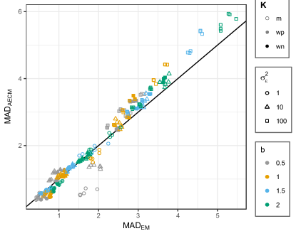
(a) $\hat{\beta}_{0}$

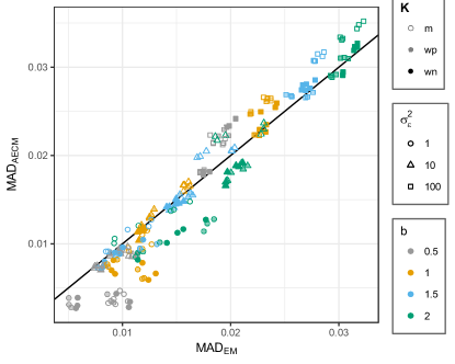
(b) $\hat{\beta}_{1}$

(c) $\hat{\boldsymbol{K}}$

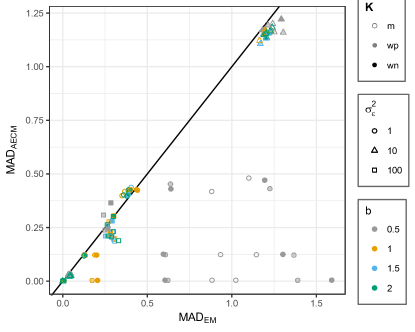
(d) $\hat{\sigma}_{\delta}^{2}$

Figure 1: Median absolute deviation of parameter estimates under the various combinations of input as described in III-A. The covariance types for $\boldsymbol{K}$ are abbreviated m = Matérn, wp = Wishart positive, and wn = Wishart negative.

Figure 1 displays the results: we see that parameters that are part of the mean structure exhibit similar patterns. The error in slope and intercept estimation is decreased by the AECM algorithm in the presence of low measurement variance ($\sigma_{\epsilon}^{2}=1$) and increased given high measurement variance ($\sigma_{\epsilon}^{2}=100$). The magnitude of deviation is also an increasing function of measurement error for either approach. The AECM algorithm decreases the error in estimating $\beta_{0}$ when the true value of $b$ is not equal to 1.5, provided the measurement error is low. When $\sigma_{\epsilon}^{2}=10$, both approaches perform similarly and when $\sigma_{\epsilon}^{2}=100$, again, the AECM algorithm exhibits signs of overfitting. This pattern is also present in estimation of $\beta_{1}$, however the relative improvement by the AECM algorithm is larger. When $\sigma_{\epsilon}^{2}$ is less than 100 and the covariance of $\boldsymbol{K}$ is nonstationary, the AECM algorithm consistently improves estimation of $\beta_{1}$. These results hold even when we vary covariance type, fine-scale variation, and sampling design.

Figure 1c shows the MAD for all unique elements of $\hat{\boldsymbol{K}}$. Most are fairly similar between the AECM and EM approaches, but there are some overall patterns that we notice. Specifically, in the presence of large measurement error or when the true $b$ is at least 1.5, the EM algorithm reduces the MAD. When the true spatial range is small and measurement error does not overwhelm the signal (i.e., $b\leq 1$ and $\sigma_{\epsilon}^{2}\leq 10$) however, the AECM algorithm typically performs better. Surprisingly, this reduction in MAD is more consistent when $b=0.5$ than when $b=1$. Again, these trends hold irrespective of covariance type, fine-scale variation, and sampling design.

Accurate estimation of variance parameters in spatial fields can often be challenging. In particular, the fine-scale variation parameter in the SME model is often underestimated. However, allowing a more flexible spatial structure by estimating the range parameter with respect to the knots ($b$) provides consistent reduction in the MAD for $\sigma_{\delta}^{2}$. Only when both independent variance components are equal ($\sigma_{\delta}^{2}=\sigma_{\epsilon}^{2}$) and occasionally when the measurement error is high does the AECM method fail to improve estimation.

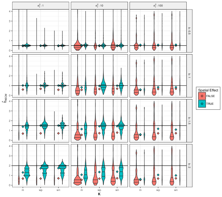
Figure 2: Distributions of $\hat{b}$ provided by the AECM. The mean of each distribution is identified by a diamond and its quartiles by horizontal black lines.

Clearly, when observations contain extreme levels of measurement error, parameter estimation given a SME model is problematic. Assuming any spatial model when non-spatial variance components dominate the total variance can have ill-effects on estimation accuracy. This is no more evident than when exploring distributions of $\hat{b}$ obtained through simulation, provided in Figure 2. Distributions are further segregated and color coded between those that showed signification spatial autocorrelation ($\alpha<.05$) as measured by [44]’s I and those that did not. (Note that some distributions of $\hat{b}$ are truncated in order to highlight the range of highest density within each distribution, however these estimates account for less than 0.17% of the total simulations.) We see in the figure that there is a clear distinction between distributions with and without significant spatial autocorrelation. When $\sigma_{\epsilon}^{2}=100$, nearly all simulated fields do not exhibit enough spatial dependence to compensate for the large measurement error. Without significant spatial dependence, $\hat{b}$’s tend to be negatively biased with a large percentage of the distribution residing between 0 and 1, made worse when $\boldsymbol{K}$ has a Matérn structure. This pattern persists for all levels of measurement error, however the percentage of fields with insignificant spatial dependence decreases with decreasing $\sigma_{\epsilon}^{2}$. Estimation of $b$ performs fairly well for true values of $b\leq 1.5$, however when $b=2$, there is again a tendency for $\hat{b}$ to be underestimated.

The difference between the estimation methods clearly varies across parameters. To summarize the fit of all parameter estimates and, consequently, the overall model fit, we compared Kullback-Leibler (KL) divergence between the two methods. KL divergence quantifies the amount of information lost when an estimated distribution, $Q$, is used in place of the true distribution, $P$. The KL divergence [25] for two multivariate normal distributions, $P\equiv N(\boldsymbol{\mu}_{P},\boldsymbol{\Sigma}_{P})$ and $Q\equiv N(\boldsymbol{\mu}_{Q},\boldsymbol{\Sigma}_{Q})$, on $\mathbb{R}^{n}$ simplifies to $2\mbox{KL}(P,Q)=\mbox{tr}(\boldsymbol{\Sigma}_{Q}^{-1}\boldsymbol{\Sigma}_{P})+(\boldsymbol{\mu}_{Q}-\boldsymbol{\mu}_{P})^{\prime}\boldsymbol{\Sigma}_{Q}^{-1}(\boldsymbol{\mu}_{Q}-\boldsymbol{\mu}_{P})-\log|\boldsymbol{\Sigma}_{P}|+\log|\boldsymbol{\Sigma}_{P}|-n.$To summarize results, Figure 3 provides the proportion out of 1000 simulations where the KL divergence is less for AECM than it is for EM. Thus, values over 0.5 indicate an improvement in overall model fit when estimating $b$.

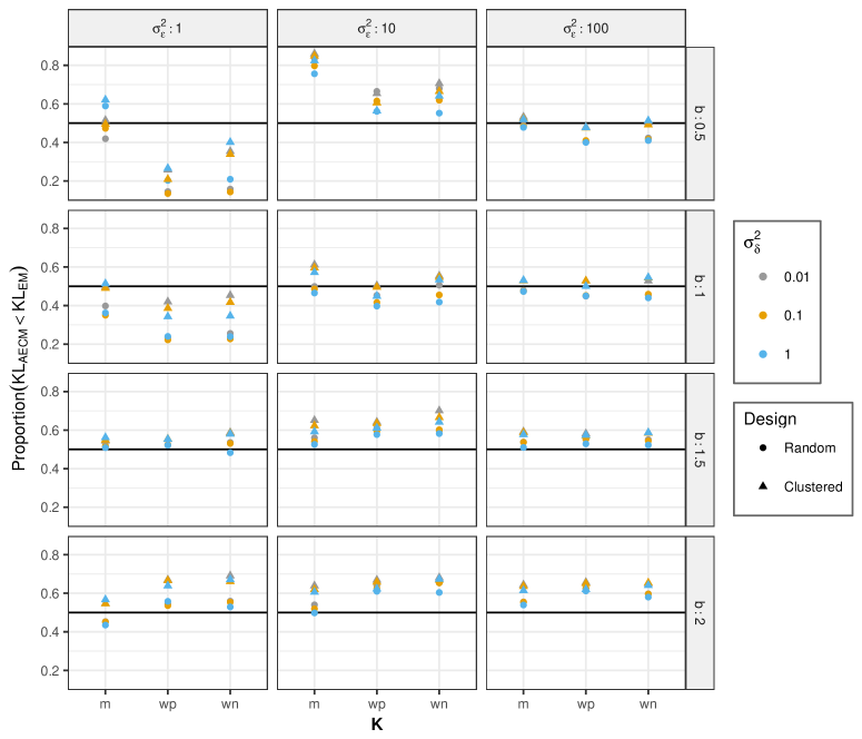
Figure 3: The proportion of simulations where the KL divergence was smaller for the AECM method than the EM method.

Interestingly, although individual parameter estimates almost unanimously improved using AECM when $b\leq 1$ and $\sigma_{\epsilon}^{2}=1$, the opposite holds when comparing KL divergence. In these cases, overall model fit is better assuming a fixed $b=1.5$. When $b\geq 1.5$, on the contrary, nearly every combination of simulation input resulted in a reduced KL divergence using the AECM algorithm. In the presence of high measurement errors, results were similar between estimating $b$ and leaving it fixed at 1.5, regardless of the true value of $b$. When $\sigma_{\epsilon}^{2}=10$, the AECM algorithm decreases KL divergence the most consistently, reaching a proportion as high as 0.86.

Our final performance comparisons were in the context of prediction. To that end, we summarized our results into three metrics: mean square prediction error (MSPE), ratio of KSE, and prediction interval coverage (PIC). MSPE is the usual statistical summary which calculates the average squared loss between the kriging predictions and the true value at unobserved locations. Since this is a simulation setting, we can define the true value as the uncorrupted spatial process, $\{\boldsymbol{y}(\boldsymbol{s}_{0})-\boldsymbol{\epsilon}(\boldsymbol{s}_{0})\}$. The median KSE at each spatial location is computed given estimated parameters by either method. The ratio KSE (rKSE) is the ratio between this median KSE and the KSE computed given the true parameter values at similar simulation input values. Ideally, the rKSE is equal to 1. PIC is the percentage of prediction intervals that contain the true value, averaged over all locations. Since we assumed 95% prediction intervals, we expect the PIC to be roughly 0.95 for each case. For each summary statistic, the median was computed over all values of $\sigma_{\delta}^{2}$ and sampling designs and results are provided in Table 1. Medians for every unique combination of input values are provided in Section S-1.1 of the Supplementary Materials.

TABLE I: Median predictions results, comparing mean square prediction error (MSPE), ratio of median estimated versus true KSE, and prediction interval coverage (PIC).

				MSPE		rKSE			PIC
K	$\sigma_{\epsilon}^{2}$	$b$	True	AE	EM	AE	EM	True	AE	EM
M	1	0.5	0.27	0.51	1.69	0.62	1.90	0.92	0.67	0.89
M	1	1	0.22	0.36	0.37	0.59	0.70	0.94	0.67	0.72
M	1	1.5	0.19	0.33	0.26	0.60	0.61	0.94	0.69	0.72
M	1	2	0.16	0.33	0.29	0.63	0.66	0.94	0.68	0.73
M	10	0.5	0.81	1.73	2.29	0.59	0.82	0.90	0.59	0.62
M	10	1	0.91	1.70	1.33	0.51	0.57	0.95	0.60	0.67
M	10	1.5	0.83	1.70	1.26	0.54	0.59	0.95	0.60	0.68
M	10	2	0.75	1.68	1.29	0.57	0.63	0.95	0.61	0.68
M	100	0.5	1.86	9.45	6.95	0.68	0.68	0.84	0.46	0.48
M	100	1	2.63	9.38	5.90	0.51	0.51	0.95	0.45	0.53
M	100	1.5	2.83	9.41	5.89	0.48	0.50	0.95	0.46	0.54
M	100	2	2.76	9.50	6.01	0.48	0.51	0.95	0.46	0.54
P	1	0.5	0.65	1.05	2.41	0.69	1.76	0.92	0.68	0.89
P	1	1	0.22	0.34	0.86	0.65	0.97	0.94	0.71	0.78
P	1	1.5	0.22	0.33	0.27	0.62	0.62	0.95	0.72	0.75
P	1	2	0.17	0.33	0.32	0.66	0.73	0.95	0.72	0.75
P	10	0.5	1.21	2.30	3.18	0.60	0.85	0.90	0.59	0.62
P	10	1	1.14	1.92	1.71	0.53	0.60	0.95	0.60	0.65
P	10	1.5	1.04	1.81	1.35	0.57	0.59	0.95	0.62	0.68
P	10	2	0.81	1.87	1.36	0.60	0.63	0.95	0.62	0.68
P	100	0.5	2.78	12.81	8.90	0.65	0.75	0.84	0.44	0.50
P	100	1	3.63	12.34	7.64	0.48	0.54	0.90	0.45	0.56
P	100	1.5	3.38	11.37	6.99	0.48	0.53	0.92	0.46	0.57
P	100	2	2.81	11.67	6.90	0.48	0.54	0.93	0.47	0.58
N	1	0.5	0.54	1.00	2.32	0.69	1.77	0.93	0.67	0.89
N	1	1	0.22	0.34	0.88	0.65	0.97	0.94	0.71	0.78
N	1	1.5	0.22	0.32	0.26	0.63	0.62	0.95	0.72	0.75
N	1	2	0.17	0.33	0.32	0.67	0.74	0.95	0.72	0.75
N	10	0.5	1.21	2.33	3.13	0.60	0.85	0.90	0.58	0.61
N	10	1	1.13	1.93	1.74	0.56	0.61	0.94	0.61	0.64
N	10	1.5	1.02	1.84	1.36	0.58	0.60	0.95	0.62	0.68
N	10	2	0.77	1.85	1.36	0.62	0.65	0.95	0.63	0.68
N	100	0.5	2.84	12.96	8.89	0.65	0.74	0.85	0.45	0.51
N	100	1	3.65	12.36	7.63	0.49	0.54	0.90	0.46	0.56
N	100	1.5	3.37	12.04	6.96	0.48	0.53	0.92	0.46	0.57
N	100	2	2.93	11.85	6.96	0.49	0.54	0.93	0.47	0.58

Clearly, knowing the true parameter values improves prediction, as its MSPE is always lowest. If the measurement error is small enough and the true $b\leq 1$, the AECM algorithm improves MSPE compared to the EM approach. However, for $\sigma_{\epsilon}^{2}\geq 10$, holding $b=1.5$ fixed provides the most accurate prediction. The KSE is often underestimated, with the AECM method exacerbating the issue. However, when the true $b=0.5$ and $\sigma_{\epsilon}^{2}=1$, the EM approach severely overestimates KSE. The lower KSE also has the consequence of lowering the PIC, as narrower confidence bands will inevitably miss the true values at a higher rate. However, the anticipated improved performance using AECM when $b=0.5$ and $\sigma_{\epsilon}^{2}=1$ is absent. To elucidate this pattern, a single realization from our simulation with prediction regions is provided in Figure 4, with the prediction interval coverage (PIC) at each location included to facilitate comparison. The PIC is exclusively closer to 0.95 for the EM method across locations (top plot), but as a plot of the actual process (bottom) accentuates, the EM method misses clear signals in the data by over-smoothing predictions. Overestimating KSE, in this case, allows the prediction intervals to include the true values, however, it is an inaccurate representation of the process.

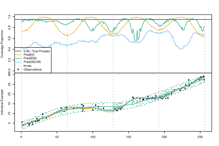
Figure 4: Simulated 1-dimensional spatial field where $b=0.5$, $\sigma_{\delta}^{2}=0.01$, $\sigma_{\epsilon}^{2}=1$, $\boldsymbol{K}\sim W_{p}(\ldots)$, and observations are randomly dispersed. The top plot shows the PIC, computed over all 1000 simulations, while the bottom plot depicts a single realization.

In summary, the results of our experiments show that estimating the bandwidth constant in the local bisquare basis functions by means of the AECM algorithm can be advantageous to both individual parameter estimation and prediction when the true $b$ is small, particularly when the measurement error is also low. This combination produces obvious large-scale trends in the data that is not captured by the mean structure. Clearly, fitting a more complex model for the mean, such as a higher order polynomial, would also allow the flexibility necessary to fit such models. The decision of whether or not to estimate $b$ is then analogous to a common statistical concern in mixed models of whether to treat an effect as fixed (mean structure) or random (spatial process), which depends on the context and desired interpretation. As expected, our results as $b$ approaches 1.5 confirm that the extra parameter estimation is unnecessary, however the potential negative effects on prediction accuracy are fairly minimal. In terms of overall model fit, as measured by KL divergence, estimating $b$ by means of the AECM algorithm still shows improvement over the standard approach of fixing $b=1.5$. Having gained these insights from our simulation study, we now apply our methodology to the National Climate Data Center (NCDC) data of monthly temperatures recorded across the continental United States of America.

IV Application: Predicting temperatures over the contiguous United States

We applied our methodology to temperature data recorded by the Cooperative Observer Program (COOP). Established in 1890, The COOP is the largest and oldest weather and climate observation network [45], recording weather information every 24 hours from over 11,700 volunteer citizens and institutions. The data are available online at the Uniform Resource Locator http://www.image.ucar.edu/Data/US.monthly.met/. Note that there is considerable variability in the number of weather stations across the contiguous United States (US) for which measurements are available at any point of time as well as in the number of variables recorded (monthly maximum temperature, minimum temperature, precipitation, etc.) at these time points.

Mean temperature recorded over a regular grid is an important summary in climate science [46], as it is used to assess the value of climate-derived models by means of comparison. Inevitably, temperatures are not recorded for all locations on the predetermined regular grid. Thus, kriging is necessary to estimate temperatures at the remaining unobserved locations. Also, since spatial dependence typically exhibits a high degree of smoothness with respect to temperature, this response should help determine if $b=1.5$ is a good default smoothing parameter value.

We restrict our attention to mean daily temperature readings for April 1990 in this paper. The COOP had daily minimum and maximum temperatures recorded at 5,030 locations across the contiguous US – these were summarized into a single univariate measurement at each of these locations in terms of an average of the mean monthly minimum and maximum temperatures. In this setup, note that performing kriging requires iteratively solving a $5030\times 5030$ linear system, a task which would be computationally prohibitive in terms of CPU time and memory. Thus, efficient forms of kriging such as fixed rank kriging, with parameter estimation achieved through either an EM or AECM approach are necessary. Note, also that this dataset is used simply for illustration, our method can easily be applied to larger sample sizes, as it is scalable with computational cost growing at a linear rate with the sample size.

IV-A Known Covariates

Temperature is known to be affected by geographic location and elevation. Since temperature cannot reasonably be modeled with a constant mean structure in the presence of these factors, a set of covariates is necessary to reduce the remaining structure to a zero-mean spatial process and zero-mean measurement error. Assuming linearity in the effects of our covariates, we can model the non-zero mean structure with the additive model $\boldsymbol{x}(\boldsymbol{s},\boldsymbol{h}_{\boldsymbol{s}})^{\prime}\boldsymbol{\beta}=\beta_{0}+\boldsymbol{g}_{Elev}(\boldsymbol{h}_{\boldsymbol{s}})\boldsymbol{\beta}_{Elev}+\boldsymbol{g}_{Lat}(\boldsymbol{s})\boldsymbol{\beta}_{Lat}+\boldsymbol{g}_{Lon}(\boldsymbol{s})\boldsymbol{\beta}_{Lon}$ where $\boldsymbol{h}_{\boldsymbol{s}}$ is the elevation at location $\boldsymbol{s}$.

The exact functional relationship between temperature and our covariates is unknown, however we expect temperature to decrease with increasing elevation and latitude. One option is to assume a simple linear mean structure for all covariates. However, this is likely an oversimplification and, hence, smoothing regression splines fit based on AIC were also used to model the mean structure. Specifically, $\boldsymbol{g}_{Elev}(\boldsymbol{h}_{\boldsymbol{s}})$ required a cubic regression spline with nine degrees of freedom, $\boldsymbol{g}_{Lat}(\boldsymbol{s})$ was modeled with a quadratic regression spline with four degrees of freedom, and $\boldsymbol{g}_{Lon}(\boldsymbol{s})$ fit best with a cubic regression spline with nine degrees of freedom. Since the AECM method showed the ability to accommodate irregular patterns in the data not captured by the mean structure, we are interested in a comparison between these “reduced” and “full” models. The model fits and their resulting residuals, are shown in Figures 5 and 6, respectively. Although the relationship between temperature and each covariate appears decidedly non-linear, validation of model assumptions, by way of a residual plot, does not feature this violation. Visual assessment suggests that both mean structures are reasonable.

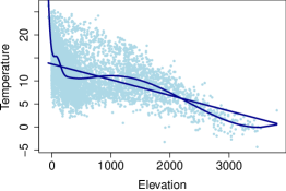
(a) Cubic spline

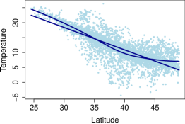
(b) Quadratic spline

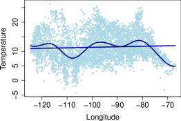
(c) Cubic spline

Figure 5: (a) - (c) display monthly mean temperature plotted against one of three covariates with linear fits and regression splines.

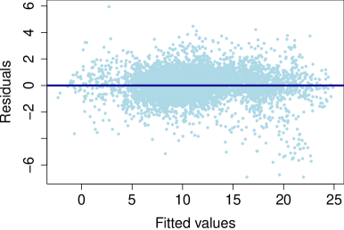
(a) Full model

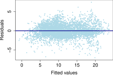
(b) Reduced model

Figure 6: Residual plots based on a fit using (a) splines and (b) a linear model.

IV-B Results and Analysis

REML estimation was carried out by maximizing the restricted log-likelihood (15) by the algorithm outlined in Section II-C and by the iterative updating scheme of (I-A) obtained by the EM algorithm. Following the strategy proposed by [29], $\sigma_{\epsilon}^{2}=2.059$ was independently determined. We selected $m=369$ knots representing 7.3% of the original data set on a regular triangular grid within a space-filling framework and tested our methodology on up to four levels of resolution. Distance matrices were obtained by using the function rdist.earth, which computes the Great circle distance between any two locations on the Earth.

The size of this dataset, despite making use of the fixed rank kriging equations, also warranted the use of more efficient software. Functions were translated to MATLAB [47], which is optimized for matrix and vector algebra and can be easily parallelized. We note that a major burden of the AECM method is that every iteration during parameter estimation costs three to four times that of the EM method and that subsequent iterations require previous results, so care had to be taken in parallelization. However, despite the additional burden, recall that the main benefit of our AECM algorithm is additional parameter estimation.

We compared model performance (a) in terms of prediction by MSPE through five-fold cross-validation and (b) in terms of efficiency, summarized by the elapsed time for estimation, in minutes (see Table 2). All reported computations was performed using a standard desktop computer with 16GB of RAM and a 64-bit Intel quad-core i7 processor. Also included in the table are parameter estimates for $b$, the range of $\boldsymbol{K}$, and $\sigma_{\delta}^{2}$ and the corresponding evaluated log-likelihood.

TABLE II: Prediction and estimation results from both the EM and AECM algorithms, using 1 to 4 resolutions ($\varrho$) and the full (top block) or reduced (bottom block) model on the US temperature dataset. The model column provides both the model and resolution. R($\hat{\boldsymbol{K}}$) represents the range of values in the $\hat{\boldsymbol{K}}$ matrix.

$\varrho$	Method	MSPE	Min.	$\hat{b}$	R($\hat{\boldsymbol{K}}$)	1E3 $\widehat{\sigma_{\delta}^{2}}$	$\ell(\hat{\boldsymbol{\theta}})$
1	EM	0.771	14.6	NA	158.64	0.0046	-7215.7
1	AECM	0.772	26.2	1.51	155.26	0.0046	-7215.8
2	EM	0.767	16.8	NA	210.11	0.0047	-7213.0
2	AECM	0.767	27.3	1.47	203.06	0.0047	-7212.6
3	EM	0.768	17.1	NA	318.34	0.0046	-7214.7
3	AECM	0.769	28.3	1.47	318.27	0.0046	-7215.2
4	EM	0.768	19.0	NA	326.18	0.0046	-7214.9
4	AECM	0.770	32.5	1.48	336.32	0.0046	-7216.3
1	EM	0.805	23.0	NA	537.85	0.0030	-7257.4
1	AECM	0.790	37.0	1.89	297.90	0.0034	-7244.9
2	EM	0.795	25.8	NA	507.49	0.0031	-7245.3
2	AECM	0.792	39.7	1.55	603.01	0.0033	-7242.1
3	EM	0.793	30.3	NA	575.08	0.0030	-7244.8
3	AECM	0.795	47.8	1.27	372.84	0.0033	-7245.4
4	EM	0.794	27.4	NA	617.49	0.0030	-7245.6
4	AECM	0.798	41.1	1.28	354.57	0.0032	-7245.1

The performance measures show that, as expected, predictions stemming from the full model provide lower MSPEs. When using the full model, 2 resolutions minimized the MSPE, with the AECM method barely outperforming the EM method. Three and two resolutions were optimal when using the reduced linear model for the EM and AECM methods, respectively. Here again, AECM produced lower prediction errors. The largest discrepancy occurred for the simplest model, reduced with only one resolution, where the AECM approach substantially decreased MSPE, relative to the EM. Although the AECM algorithm is not optimal across the board for every number of resolutions, these results also indicate that prediction error is not substantially increased.

The EM method is, by design, a more efficient algorithm and the timing results substantiate that fact. Although the AECM method does require additional computation time, the increase observed was only between 50% and 79%. Considering the amount of communication required between workers (necessary after each iteration), MATLAB manages this extra burden surprisingly well. Also note that the relative increase was lower across all resolutions when assuming the reduced model.

For the full model, parameter estimates for $\sigma_{\delta}^{2}$ were essentially identical between the two methods and estimation of $b$ validated the reasonable choice of bandwidth constant being 1.5, as mentioned by [18]. However, the resolution that both maximized the evaluated log-likelihood and minimized the MSPE also provided an estimate of $b$ with the largest deviation from 1.5. The reduced model produced estimates of $b$ as high as 1.890, with the optimal resolution, as measured by evaluated log-likelihood, estimating $b$ at 1.546. All values of $\hat{\sigma}_{\delta}^{2}$ for the reduced model are lower relative to the full model, but the decrease is consistently less for the AECM method. If we assume that the full model is a more appropriate description of our data, then this provides evidence that the AECM method counteracts the effects of model misspecification by allowing the range of the basis functions, or bandwidth, to vary. The range of $\hat{\boldsymbol{K}}$ using the AECM method also shows greater agreement between analogous models for almost every resolution, further corroborating this hypothesis. Complete image plots of $\hat{\boldsymbol{K}}$ are provided in Section S-1.2 of the Supplementary Materials.

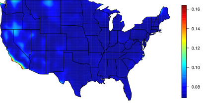
(a) EM

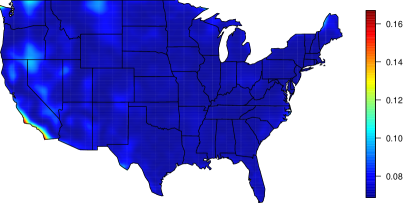
(b) AECM

Figure 7: Kriging standard errors assuming the full model with 2 resolutions for both the (a) EM and (b) AECM methods.

For the remainder of this section, we assume that the full model with two resolutions is our best model and, consequently, we focus on those results. Plots of the KSEs using both EM and AECM methods are provided in Figure 7. Both algorithms produce extremely similar results, however the scales are slightly shifted. The range of KSE values for the EM method is between 0.0688 and 0.1640, whereas the AECM method produces values between 0.0689 and 0.1669. Considering the evidence we observed that the fixed rank kriging approach underestimates KSE when $b\approx 1.5$, we are inclined to believe that the estimates of KSE resulting from the AECM method are likely closer to the truth. Other than this difference, the pattern of KSE is fairly consistent between methods across the entire contiguous US, with pockets of higher variability existing in the western states, particularly along the southern coast line of California.

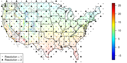
(a) Observations

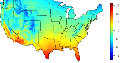
(b) Mean Structure

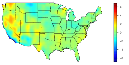
(c) Spatial Dependence

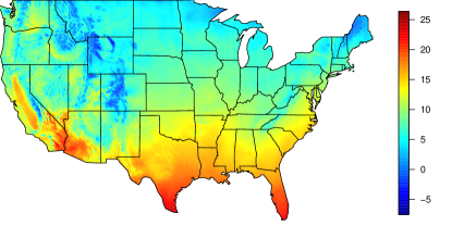
(d) Kriging Estimates

Figure 8: Mean temperatures in the US in April 1990; (a) displays the 5030 observations and 369 knots (black circles and triangles) at two resolutions, (b) shows the portion of the predicted values explained by the mean structure, (c) represents the portion of the predicted values explained by the spatial dependence, and (d) depicts the complete additive kriging estimates.

Figure 8 displays the data with superimposed knots (Figure 8a) for two resolutions and the corresponding spatially predicted field using the AECM method. The predictions are decomposed into three pieces: the mean structure ($\boldsymbol{X}(\boldsymbol{s}_{0})\hat{\boldsymbol{\beta}}$), the spatial dependence ($\boldsymbol{C}(\boldsymbol{s}_{0})\boldsymbol{\Sigma}^{-1}(\boldsymbol{y}-\boldsymbol{X}\hat{\boldsymbol{\beta}})$), and the complete additive kriging estimates ($\hat{\boldsymbol{y}}(\boldsymbol{s}_{0})=\boldsymbol{X}(\boldsymbol{s}_{0})\hat{\boldsymbol{\beta}}+\boldsymbol{C}(\boldsymbol{s}_{0})\boldsymbol{\Sigma}^{-1}(\boldsymbol{y}-\boldsymbol{X}\hat{\boldsymbol{\beta}})$). It is clear from Figure 8b that the covariates are critical to temperature prediction, since the mean structure reflects the general trends of the temperature in April in the contiguous US. In particular, the image depicts the negative relationship that exists between elevation/latitude and temperature. However, Figure 8c shows that certain geographically related aspects of temperature are not easily described by a linear function of location. Mirroring patterns of high KSE, the spatially dependent components show warmer than expected areas in Washington, Oregon, California, and along most Nevada borders. Cooler than expected regions occur mainly along the southern coast line of California and in northern Montana. The cooler California coast line relative to location can be explained by the California Current which transports northern waters southward, cooling the ocean temperature near California and, consequently, its land temperature as well [48]. The resulting complete kriging estimates are found in Figure 8d. The linear combination of the mean structure and the spatial dependence provide predictions with anticipated patterns, the mild climate relative to latitude that exists for the Pacific states being most evident. Thus, the results of applying our methodology on this dataset are explained by climate science and very encouraging.

V Discussion

This paper develops methodology to estimate a continuous tuning parameter in the SME model, analogous to the range parameter. The methodology maintains the ability to model severe nonstationarity in an efficient manner, without loss of prediction accuracy, thus making it scalable to massive data sets. This is accomplished using the SME model and fixed rank formulas developed by [18] and the EM algorithm to obtain ML estimates of the parameters in the variance structure, suggested by [27]. In addition to estimating variance components associated with the knots and fine-scale variation ($\boldsymbol{K}$ and $\sigma_{\delta}^{2}$), we estimate the range parameter in the basis functions by using the AECM algorithm. By making use of simple parallel processing options in MATLAB, we minimize the computational burden of additional parameter estimation.

Estimation of $b$ is valuable because knowledge of the range parameter in a spatial process can be of scientific interest. Our argument is that, in addition to knowledge gained about the spatial process, estimating $b$ can improve estimation of other parameters. By estimating $b$, we infuse flexibility into the model that allows the basis functions to describe the optimal range of spatial dependence. This flexibility has even been shown to reduce MSPE under certain situations when compared to its fixed $\boldsymbol{S}$ counterpart.

Although $\boldsymbol{K}$ is completely flexible, outside of standard requirements for covariance matrices, the locations of knots and the choice of basis function impose certain assumptions about the spatial dependence. The nonstationarity of $\boldsymbol{K}$ is unconstrained, however, the pattern of nonstationarity in the full covariance $\boldsymbol{\Sigma}$ is dependent on knot location. Also, in choosing the local bisquare basis function, we are assuming that the area of spatial dependence is circular, with diameter controlled by $b$. However, if an anisotropic pattern exists in the data, it would be straightforward to replace the local bisquare basis function with something more suitable. The current restriction is that the direction and relative scale of the anisotropic behavior would need to be known or estimated outside of the AECM algorithm. Interesting directions for future work, thus, would include optimal knot location and an estimation procedure that can support multiple parameters in the basis functions. This would allow for more complex structures including, but not limited to, the estimation of the direction and scale of anisotropy and a varying range for each resolution ($b_{l}$). Thus, we see that while we have addressed the issue of computationally practical estimation and prediction in massive fields under the SME model, several questions remain that are worthy of further attention.

Supplementary Materials

S-5.1 Additional Tables and Figures

S-5.11 Experimental Evaluations

A series of simulation experiments were conducted to explore the value of estimating a continuous component of the basis functions in fixed rank kriging. In particular, the bandwidth constant $b$ in the local bisquare function was estimated using the alternating expectation conditional maximization (AECM) algorithm and compared the the expectation maximization (EM) algorithm with a fixed $b=1.5$, as suggested by [18].

Data were simulated from a one-dimensional spatial mixed effects (SME) model, similar to that used by [27]. Observed locations, $n=64$, were selected from the complete spatial domain, $\mathcal{D}=\{1,\ldots,256\}$, either completely randomly or following a clustered random sample. Five knots were used, centered at 0.5, 64.5, 128.5, 192.5, and 256.5.

We used a simple linear mean structure ($\beta_{0}=5$ and $\beta_{1}=0.08$) and varied $\boldsymbol{K}$ as either Matérn, Wishart, or Wishart with strictly positive entries. Simulation values for the fine-scale variation parameter and the measurement error were, $\sigma_{\delta}^{2}=\{0.01,0.1,1\})$ and $\sigma_{\epsilon}^{2}=\{1,10,100\}$, respectively. Additional simulation inputs include the bandwidth constant ($b=\{0.5,1,1.5,2\}$), the number of resolutions ($l=1$), and the weighting functions ($v_{\delta}(\cdot)=v_{\delta}(\cdot)=1$).

One thousand Gaussian random fields were simulated using the R [41] package fields [42] for each combination of covariance type, parameter value, and sampling design. For each simulated field, we obtained MLEs using both the AECM algorithm (estimating $b$) and the EM algorithm (leaving $b=1.5$ fixed). From these estimates, we compared model fit quantified by Kullback-Leibler divergence and calculated the corresponding kriging estimates and standard errors at all locations within $\mathcal{D}$.

TABLE S-3: Median predictions results, comparing mean square prediction error (MSPE), ratio of median estimated versus true KSE, and prediction interval coverage (PIC) for a Matérn covariance.

					MSPE		rKSE			PIC
$\sigma_{\delta}^{2}$	$\sigma_{\epsilon}^{2}$	$b$	design	True	AECM	EM	AECM	EM	True	AECM	EM
0.01	1	0.5	clus	0.201	0.436	1.660	0.616	2.885	0.845	0.626	0.825
0.01	1	0.5	rand	0.085	0.145	0.988	0.578	3.296	0.854	0.583	0.864
0.01	1	1	clus	0.120	0.248	0.275	0.533	0.591	0.944	0.591	0.594
0.01	1	1	rand	0.077	0.117	0.148	0.519	0.622	0.945	0.609	0.655
0.01	1	1.5	clus	0.092	0.230	0.159	0.550	0.580	0.946	0.600	0.667
0.01	1	1.5	rand	0.073	0.109	0.086	0.537	0.558	0.944	0.634	0.696
0.01	1	2	clus	0.067	0.224	0.197	0.610	0.659	0.956	0.607	0.638
0.01	1	2	rand	0.060	0.113	0.102	0.606	0.632	0.944	0.632	0.684
0.01	10	0.5	clus	0.509	1.420	2.365	0.494	0.497	0.774	0.470	0.344
0.01	10	0.5	rand	0.438	1.156	1.594	0.451	0.418	0.769	0.408	0.332
0.01	10	1	clus	0.604	1.436	1.138	0.331	0.457	0.944	0.436	0.495
0.01	10	1	rand	0.502	1.094	0.690	0.300	0.420	0.942	0.417	0.526
0.01	10	1.5	clus	0.490	1.456	1.023	0.371	0.507	0.954	0.444	0.527
0.01	10	1.5	rand	0.459	1.090	0.662	0.316	0.489	0.939	0.422	0.559
0.01	10	2	clus	0.409	1.462	1.079	0.406	0.542	0.953	0.452	0.514
0.01	10	2	rand	0.392	1.034	0.676	0.374	0.554	0.940	0.454	0.560
0.01	100	0.5	clus	1.442	8.372	7.465	0.556	0.623	0.746	0.382	0.431
0.01	100	0.5	rand	1.446	9.610	5.844	0.558	0.497	0.748	0.354	0.419
0.01	100	1	clus	2.207	8.448	6.252	0.300	0.415	0.952	0.370	0.448
0.01	100	1	rand	2.230	9.378	4.935	0.308	0.398	0.939	0.365	0.464
0.01	100	1.5	clus	2.438	8.405	6.458	0.291	0.421	0.952	0.372	0.456
0.01	100	1.5	rand	2.436	9.529	5.015	0.294	0.396	0.940	0.369	0.472
0.01	100	2	clus	2.400	8.565	6.592	0.290	0.418	0.949	0.370	0.456
0.01	100	2	rand	2.417	9.592	5.044	0.287	0.396	0.945	0.364	0.483
0.1	1	0.5	clus	0.269	0.523	1.732	0.579	2.041	0.940	0.658	0.858
0.1	1	0.5	rand	0.174	0.223	1.026	0.534	2.203	0.940	0.631	0.901
0.1	1	1	clus	0.216	0.362	0.382	0.597	0.662	0.954	0.664	0.684
0.1	1	1	rand	0.175	0.219	0.243	0.559	0.702	0.949	0.664	0.719
0.1	1	1.5	clus	0.193	0.329	0.265	0.616	0.597	0.951	0.674	0.706
0.1	1	1.5	rand	0.167	0.206	0.184	0.580	0.578	0.948	0.681	0.710
0.1	1	2	clus	0.161	0.335	0.304	0.626	0.635	0.952	0.675	0.698
0.1	1	2	rand	0.156	0.210	0.198	0.583	0.618	0.948	0.676	0.716
0.1	10	0.5	clus	0.620	1.551	2.442	0.626	0.811	0.870	0.624	0.627
0.1	10	0.5	rand	0.536	1.259	1.680	0.592	0.711	0.868	0.574	0.632
0.1	10	1	clus	0.686	1.573	1.227	0.504	0.594	0.949	0.621	0.670
0.1	10	1	rand	0.607	1.209	0.785	0.474	0.567	0.944	0.590	0.692
0.1	10	1.5	clus	0.570	1.529	1.126	0.524	0.654	0.953	0.615	0.688
0.1	10	1.5	rand	0.549	1.176	0.775	0.482	0.628	0.942	0.596	0.707
0.1	10	2	clus	0.501	1.543	1.178	0.564	0.698	0.956	0.624	0.686
0.1	10	2	rand	0.490	1.121	0.764	0.528	0.674	0.942	0.617	0.711
0.1	100	0.5	clus	1.496	8.350	7.602	0.624	0.655	0.802	0.440	0.464
0.1	100	0.5	rand	1.552	9.830	5.944	0.615	0.540	0.802	0.412	0.463
0.1	100	1	clus	2.331	8.652	6.363	0.348	0.449	0.952	0.437	0.498
0.1	100	1	rand	2.300	9.425	5.007	0.350	0.431	0.939	0.418	0.511
0.1	100	1.5	clus	2.529	8.526	6.600	0.333	0.448	0.952	0.430	0.504
0.1	100	1.5	rand	2.558	9.578	5.129	0.332	0.424	0.941	0.416	0.519
0.1	100	2	clus	2.497	8.721	6.707	0.330	0.445	0.950	0.434	0.505
0.1	100	2	rand	2.478	9.667	5.105	0.331	0.432	0.944	0.416	0.534
1	1	0.5	clus	1.248	1.574	2.655	0.885	1.163	0.928	0.869	0.917
1	1	0.5	rand	1.134	1.247	2.010	0.839	1.218	0.927	0.854	0.929
1	1	1	clus	1.210	1.467	1.389	0.861	0.908	0.925	0.865	0.878
1	1	1	rand	1.143	1.221	1.211	0.841	0.910	0.922	0.866	0.896
1	1	1.5	clus	1.154	1.417	1.281	0.865	0.891	0.923	0.869	0.890
1	1	1.5	rand	1.122	1.217	1.160	0.844	0.872	0.922	0.870	0.890
1	1	2	clus	1.119	1.415	1.338	0.872	0.908	0.923	0.866	0.884
1	1	2	rand	1.106	1.200	1.165	0.861	0.893	0.922	0.871	0.894
1	10	0.5	clus	1.541	2.604	3.417	0.645	0.978	0.946	0.686	0.760
1	10	0.5	rand	1.464	2.273	2.634	0.579	0.917	0.946	0.648	0.758
1	10	1	clus	1.621	2.639	2.229	0.636	0.684	0.952	0.700	0.733
1	10	1	rand	1.528	2.197	1.738	0.572	0.632	0.948	0.667	0.732
1	10	1.5	clus	1.530	2.561	2.084	0.664	0.693	0.952	0.703	0.740
1	10	1.5	rand	1.488	2.249	1.720	0.588	0.634	0.948	0.669	0.731
1	10	2	clus	1.436	2.660	2.159	0.671	0.706	0.953	0.703	0.740
1	10	2	rand	1.428	2.125	1.697	0.606	0.647	0.947	0.679	0.736
1	100	0.5	clus	2.416	9.544	8.559	0.800	0.852	0.918	0.638	0.676
1	100	0.5	rand	2.471	10.861	6.855	0.779	0.766	0.914	0.618	0.681
1	100	1	clus	3.231	9.791	7.529	0.583	0.664	0.951	0.641	0.704
1	100	1	rand	3.186	10.233	5.884	0.581	0.629	0.945	0.628	0.720
1	100	1.5	clus	3.464	9.666	7.374	0.562	0.645	0.952	0.639	0.707
1	100	1.5	rand	3.477	10.522	6.014	0.556	0.624	0.944	0.628	0.723
1	100	2	clus	3.338	9.568	7.566	0.555	0.649	0.951	0.641	0.710
1	100	2	rand	3.388	10.500	6.018	0.555	0.622	0.946	0.624	0.726

TABLE S-4: Median predictions results, comparing mean square prediction error (MSPE), ratio of median estimated versus true KSE, and prediction interval coverage (PIC) for a positive Wishart covariance.

					MSPE		rKSE			PIC
$\sigma_{\delta}^{2}$	$\sigma_{\epsilon}^{2}$	$b$	design	True	AECM	EM	AECM	EM	True	AECM	EM
0.01	1	0.5	clus	0.477	1.024	2.989	0.697	2.398	0.856	0.586	0.740
0.01	1	0.5	rand	0.067	0.110	1.245	0.596	3.971	0.857	0.546	0.909
0.01	1	1	clus	0.119	0.217	0.653	0.502	0.671	0.950	0.599	0.555
0.01	1	1	rand	0.079	0.114	0.324	0.529	1.446	0.947	0.647	0.734
0.01	1	1.5	clus	0.114	0.211	0.160	0.490	0.500	0.951	0.597	0.664
0.01	1	1.5	rand	0.077	0.114	0.091	0.563	0.575	0.954	0.696	0.726
0.01	1	2	clus	0.067	0.209	0.203	0.601	0.633	0.957	0.595	0.615
0.01	1	2	rand	0.063	0.118	0.121	0.582	0.629	0.952	0.690	0.717
0.01	10	0.5	clus	1.022	3.013	3.673	0.526	0.520	0.781	0.394	0.345
0.01	10	0.5	rand	0.551	1.379	2.126	0.474	0.513	0.784	0.397	0.316
0.01	10	1	clus	0.840	1.989	1.768	0.371	0.383	0.932	0.440	0.454
0.01	10	1	rand	0.568	1.092	1.035	0.372	0.361	0.937	0.457	0.434
0.01	10	1.5	clus	0.724	2.003	1.142	0.424	0.420	0.937	0.456	0.512
0.01	10	1.5	rand	0.510	1.016	0.740	0.393	0.393	0.946	0.486	0.524
0.01	10	2	clus	0.448	1.975	1.145	0.483	0.467	0.954	0.462	0.531
0.01	10	2	rand	0.403	1.072	0.770	0.451	0.442	0.954	0.479	0.536
0.01	100	0.5	clus	2.711	14.125	10.203	0.588	0.645	0.757	0.352	0.460
0.01	100	0.5	rand	2.220	11.455	7.379	0.487	0.615	0.762	0.319	0.408
0.01	100	1	clus	3.653	13.494	8.433	0.370	0.507	0.890	0.382	0.473
0.01	100	1	rand	3.044	10.525	6.489	0.355	0.476	0.889	0.367	0.450
0.01	100	1.5	clus	3.163	13.526	7.551	0.356	0.476	0.912	0.378	0.490
0.01	100	1.5	rand	2.805	10.097	5.913	0.328	0.443	0.913	0.375	0.448
0.01	100	2	clus	2.563	12.677	7.467	0.344	0.495	0.926	0.390	0.502
0.01	100	2	rand	2.448	10.370	5.930	0.308	0.409	0.933	0.371	0.471
0.1	1	0.5	clus	0.617	1.351	3.179	0.574	1.714	0.945	0.633	0.794
0.1	1	0.5	rand	0.178	0.247	1.462	0.570	2.329	0.944	0.645	0.933
0.1	1	1	clus	0.217	0.344	0.755	0.597	0.888	0.953	0.668	0.669
0.1	1	1	rand	0.176	0.211	0.416	0.624	1.205	0.952	0.708	0.804
0.1	1	1.5	clus	0.213	0.316	0.256	0.588	0.575	0.954	0.675	0.709
0.1	1	1.5	rand	0.176	0.214	0.190	0.626	0.612	0.952	0.723	0.741
0.1	1	2	clus	0.161	0.324	0.318	0.625	0.657	0.955	0.661	0.685
0.1	1	2	rand	0.159	0.217	0.216	0.628	0.720	0.952	0.716	0.751
0.1	10	0.5	clus	1.207	3.339	3.750	0.645	0.748	0.876	0.585	0.615
0.1	10	0.5	rand	0.623	1.469	2.213	0.623	0.831	0.882	0.582	0.672
0.1	10	1	clus	0.904	2.266	1.837	0.525	0.578	0.937	0.590	0.627
0.1	10	1	rand	0.661	1.202	1.143	0.560	0.592	0.942	0.620	0.654
0.1	10	1.5	clus	0.807	2.149	1.253	0.571	0.567	0.942	0.597	0.664
0.1	10	1.5	rand	0.617	1.106	0.833	0.561	0.560	0.949	0.660	0.706
0.1	10	2	clus	0.537	2.060	1.240	0.610	0.620	0.957	0.606	0.676
0.1	10	2	rand	0.501	1.157	0.862	0.595	0.609	0.956	0.656	0.720
0.1	100	0.5	clus	2.858	13.896	10.354	0.653	0.683	0.813	0.425	0.482
0.1	100	0.5	rand	2.297	11.898	7.632	0.575	0.677	0.823	0.386	0.450
0.1	100	1	clus	3.707	13.924	8.734	0.408	0.523	0.895	0.438	0.508
0.1	100	1	rand	2.980	10.811	6.502	0.408	0.496	0.892	0.425	0.492
0.1	100	1.5	clus	3.235	13.385	7.728	0.401	0.508	0.916	0.438	0.532
0.1	100	1.5	rand	2.916	10.334	6.012	0.377	0.476	0.916	0.420	0.500
0.1	100	2	clus	2.669	12.698	7.707	0.380	0.511	0.931	0.448	0.542
0.1	100	2	rand	2.569	10.449	5.963	0.355	0.441	0.931	0.430	0.514
1	1	0.5	clus	1.575	2.354	4.084	0.870	1.079	0.930	0.864	0.897
1	1	0.5	rand	1.145	1.264	2.466	0.856	1.260	0.930	0.861	0.938
1	1	1	clus	1.240	1.459	1.773	0.851	0.945	0.925	0.860	0.870
1	1	1	rand	1.144	1.223	1.400	0.861	0.998	0.924	0.873	0.906
1	1	1.5	clus	1.218	1.411	1.281	0.854	0.875	0.923	0.866	0.889
1	1	1.5	rand	1.134	1.206	1.168	0.860	0.877	0.923	0.877	0.893
1	1	2	clus	1.114	1.412	1.328	0.871	0.900	0.923	0.867	0.887
1	1	2	rand	1.109	1.221	1.194	0.865	0.907	0.925	0.878	0.898
1	10	0.5	clus	2.059	4.285	4.822	0.639	0.868	0.951	0.671	0.738
1	10	0.5	rand	1.581	2.482	3.186	0.588	1.056	0.950	0.660	0.790
1	10	1	clus	1.924	3.353	2.844	0.630	0.671	0.952	0.686	0.713
1	10	1	rand	1.595	2.223	2.111	0.623	0.747	0.951	0.694	0.752
1	10	1.5	clus	1.741	3.235	2.255	0.623	0.635	0.953	0.686	0.726
1	10	1.5	rand	1.545	2.087	1.820	0.648	0.654	0.954	0.715	0.748
1	10	2	clus	1.471	3.164	2.228	0.667	0.680	0.953	0.693	0.730
1	10	2	rand	1.442	2.174	1.819	0.663	0.680	0.953	0.716	0.757
1	100	0.5	clus	3.724	14.839	10.887	0.804	0.859	0.928	0.624	0.666
1	100	0.5	rand	3.213	12.601	8.405	0.768	0.881	0.929	0.615	0.677
1	100	1	clus	4.561	14.698	9.633	0.635	0.701	0.920	0.631	0.694
1	100	1	rand	3.950	11.737	7.406	0.642	0.695	0.919	0.624	0.702
1	100	1.5	clus	4.211	14.104	8.698	0.647	0.695	0.931	0.622	0.685
1	100	1.5	rand	3.803	11.181	6.954	0.638	0.693	0.932	0.628	0.710
1	100	2	clus	3.634	13.968	8.757	0.624	0.696	0.940	0.636	0.705
1	100	2	rand	3.567	11.602	7.010	0.610	0.659	0.942	0.637	0.719

TABLE S-5: Median predictions results, comparing mean square prediction error (MSPE), ratio of median estimated versus true KSE, and prediction interval coverage (PIC) for a Wishart covariance.

					MSPE		rKSE			PIC
$\sigma_{\delta}^{2}$	$\sigma_{\epsilon}^{2}$	$b$	design	True	AECM	EM	AECM	EM	True	AECM	EM
0.01	1	0.5	clus	0.586	1.579	3.139	0.689	2.380	0.856	0.576	0.709
0.01	1	0.5	rand	0.082	0.140	1.342	0.645	3.727	0.854	0.568	0.907
0.01	1	1	clus	0.123	0.236	0.654	0.499	0.662	0.947	0.591	0.560
0.01	1	1	rand	0.080	0.110	0.313	0.530	1.353	0.947	0.664	0.732
0.01	1	1.5	clus	0.114	0.219	0.169	0.481	0.493	0.954	0.605	0.655
0.01	1	1.5	rand	0.079	0.109	0.095	0.568	0.579	0.958	0.694	0.745
0.01	1	2	clus	0.069	0.219	0.218	0.587	0.611	0.954	0.587	0.626
0.01	1	2	rand	0.067	0.119	0.117	0.565	0.608	0.953	0.680	0.711
0.01	10	0.5	clus	1.093	2.790	3.987	0.503	0.529	0.784	0.394	0.350
0.01	10	0.5	rand	0.546	1.332	2.121	0.463	0.501	0.784	0.387	0.320
0.01	10	1	clus	0.855	1.979	1.665	0.352	0.364	0.941	0.424	0.467
0.01	10	1	rand	0.587	1.152	1.040	0.333	0.340	0.943	0.432	0.442
0.01	10	1.5	clus	0.719	1.831	1.114	0.390	0.396	0.943	0.444	0.508
0.01	10	1.5	rand	0.543	1.074	0.734	0.380	0.382	0.955	0.454	0.518
0.01	10	2	clus	0.478	1.794	1.140	0.463	0.440	0.958	0.454	0.529
0.01	10	2	rand	0.442	1.131	0.755	0.430	0.430	0.954	0.462	0.528
0.01	100	0.5	clus	2.681	13.242	10.101	0.593	0.639	0.758	0.336	0.444
0.01	100	0.5	rand	2.204	11.911	7.389	0.514	0.675	0.769	0.318	0.424
0.01	100	1	clus	3.582	13.106	8.480	0.348	0.503	0.888	0.370	0.471
0.01	100	1	rand	2.957	10.930	6.383	0.327	0.462	0.888	0.346	0.448
0.01	100	1.5	clus	3.216	11.952	7.602	0.348	0.501	0.908	0.378	0.500
0.01	100	1.5	rand	2.751	10.207	5.883	0.322	0.456	0.914	0.368	0.452
0.01	100	2	clus	2.483	12.425	7.471	0.338	0.510	0.920	0.384	0.487
0.01	100	2	rand	2.385	10.409	5.858	0.328	0.436	0.926	0.370	0.458
0.1	1	0.5	clus	0.684	1.390	3.265	0.612	1.725	0.940	0.643	0.786
0.1	1	0.5	rand	0.178	0.242	1.487	0.596	2.357	0.939	0.655	0.925
0.1	1	1	clus	0.214	0.344	0.739	0.603	0.916	0.954	0.674	0.679
0.1	1	1	rand	0.177	0.206	0.406	0.612	1.187	0.953	0.709	0.809
0.1	1	1.5	clus	0.213	0.326	0.264	0.574	0.574	0.954	0.670	0.697
0.1	1	1.5	rand	0.178	0.214	0.192	0.623	0.617	0.953	0.720	0.743
0.1	1	2	clus	0.164	0.318	0.323	0.627	0.661	0.954	0.668	0.700
0.1	1	2	rand	0.161	0.222	0.216	0.611	0.705	0.952	0.717	0.751
0.1	10	0.5	clus	1.166	2.998	4.082	0.650	0.744	0.870	0.586	0.616
0.1	10	0.5	rand	0.617	1.448	2.253	0.621	0.811	0.880	0.587	0.664
0.1	10	1	clus	0.951	2.085	1.752	0.504	0.548	0.946	0.583	0.643
0.1	10	1	rand	0.666	1.240	1.131	0.515	0.536	0.947	0.607	0.657
0.1	10	1.5	clus	0.826	1.959	1.216	0.527	0.543	0.946	0.586	0.663
0.1	10	1.5	rand	0.636	1.178	0.854	0.546	0.540	0.956	0.647	0.702
0.1	10	2	clus	0.571	1.955	1.234	0.593	0.593	0.958	0.603	0.675
0.1	10	2	rand	0.530	1.237	0.849	0.576	0.591	0.955	0.644	0.714
0.1	100	0.5	clus	2.728	13.341	10.273	0.651	0.685	0.819	0.424	0.480
0.1	100	0.5	rand	2.282	11.977	7.594	0.582	0.695	0.822	0.392	0.454
0.1	100	1	clus	3.668	13.421	8.622	0.409	0.528	0.892	0.435	0.496
0.1	100	1	rand	3.052	10.900	6.405	0.384	0.498	0.893	0.412	0.490
0.1	100	1.5	clus	3.316	12.098	7.664	0.398	0.523	0.910	0.438	0.524
0.1	100	1.5	rand	2.889	10.246	5.987	0.375	0.485	0.916	0.418	0.486
0.1	100	2	clus	2.570	12.533	7.525	0.387	0.536	0.921	0.446	0.534
0.1	100	2	rand	2.492	10.449	5.943	0.370	0.468	0.927	0.426	0.506
1	1	0.5	clus	1.642	2.447	4.321	0.867	1.078	0.928	0.858	0.888
1	1	0.5	rand	1.150	1.271	2.414	0.865	1.263	0.928	0.862	0.940
1	1	1	clus	1.229	1.474	1.756	0.859	0.949	0.925	0.867	0.880
1	1	1	rand	1.140	1.217	1.394	0.855	0.991	0.924	0.872	0.908
1	1	1.5	clus	1.204	1.391	1.271	0.858	0.881	0.924	0.866	0.890
1	1	1.5	rand	1.136	1.207	1.168	0.860	0.885	0.923	0.879	0.894
1	1	2	clus	1.115	1.437	1.331	0.867	0.900	0.923	0.864	0.885
1	1	2	rand	1.112	1.220	1.189	0.854	0.904	0.924	0.870	0.892
1	10	0.5	clus	2.121	4.254	5.054	0.629	0.869	0.951	0.662	0.742
1	10	0.5	rand	1.590	2.466	3.171	0.607	1.048	0.950	0.657	0.790
1	10	1	clus	1.942	3.254	2.783	0.621	0.668	0.952	0.681	0.719
1	10	1	rand	1.612	2.270	2.097	0.610	0.708	0.953	0.683	0.743
1	10	1.5	clus	1.775	3.035	2.169	0.629	0.640	0.953	0.683	0.730
1	10	1.5	rand	1.574	2.157	1.803	0.644	0.644	0.954	0.707	0.753
1	10	2	clus	1.500	2.981	2.227	0.661	0.664	0.954	0.690	0.724
1	10	2	rand	1.455	2.229	1.794	0.638	0.659	0.953	0.696	0.751
1	100	0.5	clus	3.692	14.274	11.203	0.794	0.861	0.926	0.624	0.661
1	100	0.5	rand	3.210	12.881	8.484	0.757	0.884	0.932	0.605	0.674
1	100	1	clus	4.592	14.293	9.487	0.642	0.701	0.918	0.632	0.688
1	100	1	rand	3.917	11.703	7.325	0.639	0.700	0.920	0.613	0.694
1	100	1.5	clus	4.216	12.840	8.468	0.640	0.701	0.927	0.618	0.693
1	100	1.5	rand	3.817	11.379	6.975	0.627	0.685	0.933	0.627	0.704
1	100	2	clus	3.484	13.311	8.493	0.636	0.707	0.936	0.640	0.712
1	100	2	rand	3.316	11.494	6.852	0.624	0.688	0.938	0.629	0.717

S-5.12 Application: Predicting temperatures over the contiguous United States

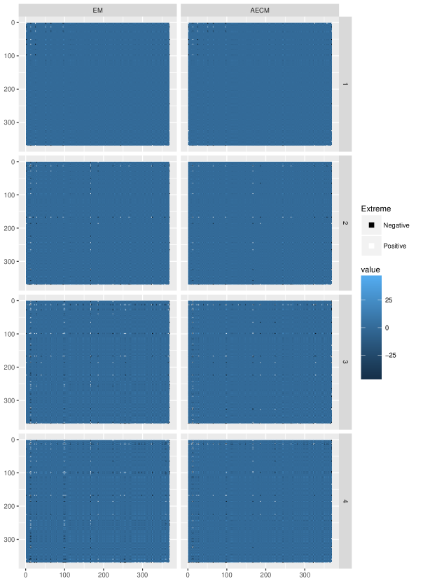
Figure S-9: $\hat{\boldsymbol{K}}$ when assuming the full model. “Extreme” values are defined as estimates beyond +/- 50.

We applied our methodology to climatological data on temperature recorded by the Cooperative Observer Program (COOP), archived at the US National Climate Data Center (NCDC) and available online at http://www.image.ucar.edu/Data/US.monthly.met/. As a response, we chose the average of mean monthly minimum and maximum temperature for April, 1990. Complete image plots of $\hat{\boldsymbol{K}}$ are provided in Figures S-9 and S-10 for the full and reduced models, respectively. In order to visually decipher smaller differences, all estimates of $\boldsymbol{K}$ such that $|\hat{K_{ij}}|>50$ are truncated.

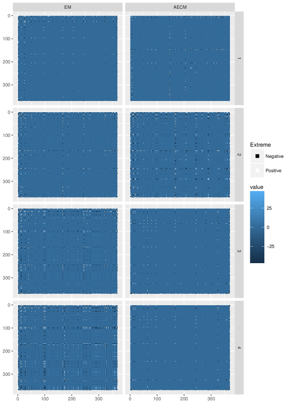
Figure S-10: $\hat{\boldsymbol{K}}$ when assuming the reduced model. “Extreme” values are defined as estimates beyond +/- 50.

These “extreme” values are then color-coded in black and white for emphasis.

References

- [1] G. Matheron, Traite de Geostatistique Applique. Technip, 1962, vol. 1.
- [2] N. Cressie, Statistics for Spatial Data, revised ed. Wiley Series in Probability and Mathematical Statistics, 1993.
- [3] A. Vecchia, “Estimation and model identification for continuous spatial processes,” Journal of the Royal Statistical Society.Series B (Methodological), pp. 297–312, 1988.
- [4] D. Nychka, B. Bailey, S. Ellner, P. Haaland, and M. O’Connell, FUNFITS: Data Analysis and Statistical Tools for Estimating Functions. Raleigh: North Carolina State University, 1996.
- [5] D. Higdon, “A process-convolution approach to modelling temperatures in the north atlantic ocean,” Environmental and Ecological Statistics, vol. 5, no. 2, pp. 173–190, 1998.
- [6] D. Nychka, “Spatial-process estimates as smoothers,” in Smoothing and Regression: Approaches, Computation, and Application, M. G. Schimek, Ed. New York: Wiley, 2000, pp. 393 – 424.
- [7] D. Nychka, C. Wikle, and J. A. Royle, “Multiresolution models for nonstationary spatial covariance functions,” Statistical Modelling, vol. 2, no. 4, pp. 315 – 331, 2002.
- [8] M. Fuentes, “Spectral methods for nonstationary spatial processes,” Biometrika, vol. 89, no. 1, pp. 197–210, 2002.
- [9] S. D. Billings, R. K. Beatson, and G. N. Newsam, “Interpolation of geophysical data using continuous global surfaces,” Geophysics, vol. 67, no. 6, pp. 1810 – 1822, 2002.
- [10] ——, “Smooth fitting of geophysical data using continuous global surfaces,” Geophysics, vol. 67, no. 6, pp. 1823 – 1834, 2002.
- [11] M. Stein, Z. Chi, and L. Welty, “Approximating likelihoods for large spatial data sets,” Journal of the Royal Statistical Society: Series B (Statistical Methodology), vol. 66, no. 2, pp. 275–296, 2004.
- [12] J. Quiñero Candela and C. Rasmussen, “A unifying view of sparse approximate Gaussian process regression,” Journal of Machine Learning Research, vol. 6, pp. 1939 – 1959, 2005.
- [13] R. Furrer, M. Genton, and D. Nychka, “Covariance tapering for interpolation of large spatial datasets,” Journal of Computational and Graphical Statistics, vol. 15, no. 3, pp. 502 – 523, 2006.
- [14] C. Kaufman, M. Schervish, and D. Nychka, “Covariance tapering for likelihood-based estimation in large spatial data sets,” Journal of the American Statistical Association, vol. 103, no. 484, pp. 1545 – 1555, 2008.
- [15] H. C. Huang, N. Cressie, and J. Gabrosek, “Fast, resolution-consistent spatial prediction of global processes from satellite data,” Journal of Computational Graphical Statistics, vol. 11, pp. 63 – 88, 2002.
- [16] G. Johannesson and N. Cressie, “Variance-covariance modeling and estimation for multi-resolution spatial models,” in geoENV IV-Geostatistics for Environmental Applications, X. Sanchez-Vila, J. Carrera, and J. Gomez-Hernandez, Eds. Dordrecht: Kluwer, 2004, pp. 319–330.
- [17] G. Johannesson, N. Cressie, and H. C. Huang, “Dynamic multi-resolution spatial models,” Environmental and Ecological Statistics, vol. 14, pp. 5–25, 2007.
- [18] N. Cressie and G. Johannesson, “Fixed rank kriging for very large spatial data sets,” Journal of the Royal Statistical Society B, vol. 70, no. 1, pp. 209 – 226, 2008.
- [19] S. Banerjee, A. Gelfand, A. Finley, and H. Sang, “Gaussian predictive process models for large spatial data sets,” Journal of the Royal Statistical Society, Series B, vol. 70, no. 4, pp. 825–848, 2008.
- [20] A. Finley, H. Sang, S. Banerjee, and A. Gelfand, “Improving the performance of predictive process modeling for large datasets,” Computational Statistics and Data Analysis, vol. 53, no. 8, pp. 2873–2884, 2008.
- [21] F. Lindgren, H. Rue, and J. Lindström, “An explicit link between Gaussian fields and Gaussian Markov random fields: the stochastic partial differential equation approach,” Journal of the Royal Statistical Society: Series B (Statistical Methodology), vol. 73, no. 4, pp. 423–498, 2011.
- [22] D. Nychka, S. Bandyopadhyay, D. Hammerling, F. Lindgren, and S. Sain, “A multiresolution Gaussian process model for the analysis of large spatial datasets,” Journal of Computational and Graphical Statistics, vol. 24, no. 2, pp. 579–599, 2015.
- [23] M. Katzfuss, “A multi-resolution approximation for massive spatial datasets,” Journal of the American Statistical Association, no. just-accepted, 2016.
- [24] J. Bradley, N. Cressie, and T. Shi, “A comparison of spatial predictors when datasets could be very large,” Statistics Surveys, vol. 10, pp. 100–131, 2016.
- [25] M. Stein, “Limitations on low rank approximations for covariance matrices of spatial data,” Spatial Statistics, vol. 8, pp. 1–19, 2014.
- [26] H. Henderson and S. Searle, “On deriving the inverse of a sum of matrices,” Society for Industrial and Applied Mathematics Review, vol. 23, no. 1, pp. 53 – 60, 1981.
- [27] M. Katzfuss and N. Cressie, “Spatio-temporal smoothing and em estimation for massive remote-sensing data sets,” Journal of Time Series Analysis, vol. 32, pp. 430–446, 2011.
- [28] A. P. Dempster, N. M. Laird, and D. B. Rubin, “Maximum likelihood for incomplete data via the em algorithm,” Jounal of the Royal Statistical Society, Series B, vol. 39, pp. 1–38, 1977.
- [29] E. Kang, N. Cressie, and T. Shi, “Using temporal variability to improve spatial mapping with application to satellite data,” Canadian Journal of Statistics, 2010.
- [30] X. Meng and D. van Dyk, “The EM algorithm–an old folk-song sung to a fast new tune,” Journal of the Royal Statistical Society, vol. 59, no. 3, pp. 511–567, 1997.
- [31] W. Chen and R. Maitra, “Model-based clustering of regression time series data via APECM – an AECM algorithm sung to an even faster beat,” Statistical Analysis and Data Mining, vol. 4, pp. 567–578, 2011.
- [32] K. Xu and C. K. Wikle, “Estimation of parameterized spatio-temporal dynamic models,” Journal of Statistical Planning and Inference, vol. 137, pp. 567–588, 2007.
- [33] T. Davis, Direct Methods for Sparse Linear Systems, ser. Fundamentals of Algorithms. Society for Industrial and Applied Mathematics, 2006.
- [34] M. Katzfuss and N. Cressie, “Maximum likelihood estimation of covariance parameters in the spatial-random-effects model,” in Proceedings of the 2009 Joint Statistical Meetings. American Statistical Association Alexandria, VA, 2009, pp. 3378–3390.
- [35] D. Harville, Matrix algebra from a statistician’s perspective. Springer, 2008.
- [36] L. Muu and N. Quy, “A global optimization method for solving convex quadratic bilevel programming problems,” Journal of Global Optimization, vol. 26, no. 2, pp. 199–219, 2003.
- [37] J. Kiefer, “Sequential minimax search for a maximum,” Proceedings of the American Mathematical Society, vol. 4, no. 3, pp. 502 – 506, 1953.
- [38] M. Avriel and D. Wilde, “Optimality proof for the symmetric Fibonacci search technique,” Fibonacci Quarterly, vol. 4, no. 3, pp. 265–269, 1966.
- [39] M. Stein, Interpolation of Spatial Data. Springer, 1999.
- [40] J. Wishart, “The generalised product moment distribution in samples from a normal multivariate population,” Biometrika, vol. 20A, no. 1/2, pp. 32 – 52, 1928.
- [41] R Core Team, R: A Language and Environment for Statistical Computing, R Foundation for Statistical Computing, Vienna, Austria, 2015. [Online]. Available: https://www.R-project.org/
- [42] D. Nychka, R. Furrer, J. Paige, and S. Sain, fields: Tools for Spatial Data, 2015, r package version 8.3-5. [Online]. Available: https://CRAN.R-project.org/package=fields
- [43] S. Kullback and R. Leibler, “On information and sufficiency,” The Annals of Mathematical Statistics, vol. 22, no. 1, pp. 79–86, 1951.
- [44] P. Moran, “Notes on continuous stochastic phenomena,” Biometrika, vol. 37, no. 1, pp. 17–23, 1950.
- [45] “Cooperative Observer Program (COOP),” 2000.
- [46] C. Johns, D. Nychka, T. Kittel, and D. C., “Infilling sparse records of spatial fields,” Journal of the American Statistical Association, vol. 98, no. 464, pp. 796 – 806, 2003.
- [47] The MathWorks, Inc., MATLAB and Statistics Toolbox Release 2014a, The MathWorks, Inc., Natick, Massachusetts, United States, 2014.
- [48] B. Hickey, “The California current system-hypotheses and facts,” Progress in Oceanography, vol. 8, no. 4, pp. 191–279, 1979.