Fibre inflation and precision CMB data

Sukannya Bhattacharya^a, Koushik Dutta^b,c, Mayukh Raj Gangopadhyay^d ,

Anshuman Maharana^e, Kajal Singh^e

^aTheoretical Physics Division, Physical Research Laboratory, Navrangpura,
Ahmedabad 380009, India
^b Indian Institute of Science Education And Research Kolkata,
Mohanpur, West Bengal 741 246, India
^cTheory Divison, Saha Institute of Nuclear Physics, HBNI,1/AF Bidhannagar,
Kolkata 700064, India
^dCentre for Theoretical Physics, Jamia Millia Islamia,
New Delhi 110025, India
^eHarish-Chandra Research Institute, HBNI, Jhunsi,
Allahabad, Uttar Pradesh 211019, India

Generic features of models of inflation obtained from string compactifications are the correlations between the model parameters and the postinflationary evolution of the universe. Thus, the postinflationary evolution depends on the inflationary model parameters and accurate inflationary predictions require that this be incorporated in the evolution of the primordial spectrum. The fibre inflation model is a promising model of inflation constructed in type IIB string theory. This model has two interesting features in its postinflationary evolution. The reheating temperature of the model is directly correlated with the model parameters. The model also necessarily predicts some dark radiation, which can be sizable for certain choices of discrete parameters in the model. We analyze this model in detail using publicly available codes - ModeChord and CosmoMC with the latest Planck+BICEP2/Keck array data to constrain the model parameters and $N_{\rm pivot}$ (the number of $e$-foldings between horizon exit of the CMB pivot mode and the end of inflation). We also carry out the same analysis using the publicly available code Cobaya. We find the results of both the analysis to be in agreement. Our analysis provides the basic methods necessary to extract precise inflationary prediction in string models incorporating correlations between model parameters and postinflationary evolution.

1 Introduction

The inflationary paradigm provides an extremely attractive explanation for the observed spectrum and inhomogeneities in the cosmic microwave background (CMB) [1]. Since observations in the future are likely to minutely probe the CMB [2], it is important to develop a systematic understanding of the methodology for extracting highly accurate predictions for inflationary models. The simplest method is to parametrize primordial perturbations with a set of empirical variables such as $A_{s}$ (the strength of the power spectrum), $n_{s}$ (the scalar tilt), $r$ (the tensor-to-scalar ratio), $f_{\rm NL}$ (parametrizing the non-Gaussianity) etc. The best-fit values of these are obtained by evolving the primordial fluctuations and comparing with observations of the CMB. Given a model of inflation, one can also compute the functional form of the primordial fluctuations in terms of the parameters of the model. One then requires that the predictions for the empirical parameters are in the best-fit regions, determined by the evolution of the initial perturbations. Note that this is intrinsically a two-step process where the empirical parameters characterizing the primordial perturbations act as the matching points between observation and theory.

On the other hand, if one wants to confront a particular model of inflation with data, a more comprehensive method is to treat the model parameters as inputs for the cosmological evolution and directly determine the best-fit regions for these parameters [3, 4] (see also [5]). This approach is particularly well suited if one is considering models which arise from a fundamental theory (such as string theory). In this case, one naturally expects various correlations between the model parameters and the postinflationary evolution of the universe. Thus, the postinflationary evolution depends on the model parameters and accurate inflationary predictions require that this be incorporated in the evolution of the primordial spectrum. Inflationary predictions of any model are sensitive to higher derivative corrections in the effective action. Hence, theories of quantum gravity are the appropriate setting to carry out inflationary model building. In this light, on can expect to use precision cosmology to confront models of quantum gravity with observations. Work in this direction, to explicitly constrain model parameters incorporating the correlations between model parameters and the postinflationary history was initiated in [6] in the context of the Kähler moduli inflation model [7].

Fibre inflation [8] is a promising model of inflation set in IIB string theory. Phenomenologically, the model is interesting as it predicts a value of the tensor to scalar ratio ($r>0.005$) which can be observationally verified with experiments planned in the near future. Thus, it is timely to carry out a detailed study of the model predictions. As we will discuss in detail in the next section, the model has two interesting features in its postinflationary evolution. The reheating temperature of the model is directly correlated with the model parameters. The model also necessarily predicts some dark radiation, which can be sizable for certain choices of discrete parameters in the model. In this paper, we use Modechord [4] and CosmoMC [9] (and also give an independent analysis using Cobaya [10]), incorporate these features in the postinflationary evolution and thereby perform a detailed analysis of the model predictions. The basic philosophy of constraining the model parameter space using precision cosmology is the same as that in [6].

These two features are also expected to be generic in string constructions. For a discussion of dark radiation in string models, see e.g. [12]. Thus, our analysis can serve as a template for the analysis of most string models. The effects of presence of dark radiation on cosmological observations are studied in [13].

Recently, the predictions of fibre inflation and their relationship to post inflationary dynamics have been analyzed in [14]. Our work develops this analysis, systematically incorporating the relationship between the model parameters and the post inflationary dynamics making use of the above-mentioned publicly available packages. This allows us to obtain a detailed understanding of the model predictions.

This paper is structured as follows. In Sec. 2, we review some basic aspects of fibre inflation; in Sec. 3 we discuss our methodology and perform our analysis; in Sec. 4 we discuss our results and conclude.

2 Review of Fibre Inflation

The fibre inflation model is set in the large volume scenario [16] for moduli stabilization of IIB flux compactifications. Here, we briefly review aspects of the model that will be needed for our analysis and refer the reader to [8, 14, 17] for further details. The relevant dynamics during the inflationary epoch is that of the Kähler moduli fields of the Calabi-Yau manifold associated with the compactification. The Kähler moduli are flat at tree level, but acquire a potential as a result of nonperturbative corrections to the superpotential, loop, and $\alpha^{\prime}$ corrections to the Kähler potential. The construction of fibre inflation models involves Calabi-Yau manifolds with at least three Kähler moduli:

• $T_{1}=\tau_{1}+i\theta_{1}$. For this field, the geometric modulus $\tau_{1}$ corresponds to the volume of a $T^{4}$ or $K3$ fibred over a $\mathbb{P}^{1}$ base. The field $\tau_{1}$ plays the role of the inflaton in the model.

• $T_{2}=\tau_{2}+i\theta_{2}$. Here the geometric modulus corresponds to the volume of the base.

• $T_{3}=\tau_{3}+i\theta_{3}$. Here, the geometric modulus corresponds to the blow-up of a pointlike singularity. Nonperturbative effects on this cycle play an important role in moduli stabilization.

The volume of the compactification can be expressed in terms of the volumes of the geometric moduli as

$${\mathcal{V}}=\alpha\left(\sqrt{\tau_{1}}\tau_{2}-\gamma\tau_{3}^{3/2}\right),$$ (2.1)

where $\alpha$ and $\gamma$ are order one constants determined by the intersection numbers of the four cycles.

The potential developed as a result of the effects described above can be expanded in an inverse volume expansion. At order ${\mathcal{V}}^{-3}$, the geometric moduli $\tau_{2}$ and $\tau_{3}$ and the axion $\theta_{3}$ are stabilized. Loop effects at order ${\mathcal{V}}^{-10/3}$ provide a potential for the field $\tau_{1}$. This takes the form (in Planck units)

$$V(\tau_{1})=\left(g_{s}^{2}{A\over\tau_{1}^{2}}-{B\over\sqrt{\tau_{1}}}+g_{s}^{2}{C\tau_{1}\over{\mathcal{V}}^{2}}\right){W_{0}^{2}\over{\mathcal{V}}^{2}},$$ (2.2)

where $W_{0}$ is the vacuum expectation value of the Gukov-Vafa-Witten superpotential and

$$A=\left(c_{1}^{\rm KK}\right)^{2}\phantom{abcdef}B=2\alpha c^{\rm W}\phantom{abcdef}\phantom{abcd}C=2(\alpha c_{2}^{\rm KK})^{2}$$

with $c_{1}^{\rm KK}$, $c_{2}^{\rm KK}$, and $c^{\rm W}$ depending on the underlying compactification and fluxes. After incorporation of effects so that the minimum is a Minkowski one, canonical normalization of $\tau_{1}$, and shifting the zero of the field to its minimum, the potential for the canonically normalized inflaton field $(\hat{\phi})$ is

$$V=V_{0}\left(3-4e^{-k\hat{\phi}}+e^{-4k\hat{\phi}}+R\left(e^{2k\hat{\phi}}-1\right)\right),$$ (2.3)

where

$$k={1\over\sqrt{3}},\phantom{abcd}V_{0}={g_{s}^{1/3}W_{0}^{2}A\over 4\pi\lambda^{2}}\phantom{abc}\textrm{with}\phantom{abc}\lambda=\left({4A\over B}\right)^{2/3},\phantom{abcd}\textrm{and}\phantom{abcd}R=16g_{s}^{4}{AC\over B^{2}}$$ (2.4)

The inflationary trajectory is such that ${\hat{\phi}}$ rolls from positive values towards its minimum at zero. Note that $R\propto g_{s}^{4}$ and hence is naturally small. The potential has two inflection points: ${\hat{\phi}}_{\rm ip}^{(1)}\sim k\ln 4$ and ${\hat{\phi}}_{\rm ip}^{(2)}\sim-k\ln R$. The second inflection point occurs as a result of competition between the positive exponential and the negative ones. Inflation occurs when the field lies between the two inflection points. If the value of $R$ is small, $R<2\times 10^{-6}$, then the horizon exit of the CMB modes takes place at a field value $({\hat{\phi}}_{*})$ which is much less than the second inflection point ${\hat{\phi}}_{*}\ll{\hat{\phi}}^{(2)}_{\rm ip}$, and the positive exponential term can be neglected. In this regime, a robust prediction of the model is a relationship between the spectral tilt $(n_{s})$ and the tensor-to-scalar ratio $(r)$

$$r=6(n_{s}-1)^{2}$$ (2.5)

On the other hand, for higher values of $R$, the horizon exit of CMB modes takes place at a point which is closer to the second inflection point; the positive exponential term has to be incorporated in the analysis. With an increase in the value of $R$, the model predicts higher values of $n_{s}$ and $r$. Also, the relationship (2.5) is broken.

The reheating epoch in fibre inflation models has been examined in detail in [14]. After the end of inflation, the inflaton oscillates about its minimum and decays perturbatively, which is supported by the full numerical analysis of the evolution of the scalar field after inflation [19] (a semianalytic approach [20] has suggested the possibility of a preheating epoch, but the evidence from the full numerical study is that the process is perturbative) . The dominant decay channels are visible sector gauge bosons, visible sector Higgs, and ultralight bulk hidden axionic fields (which act as dark radiation). The total visible sector and the hidden sector decay widths are given by

$$\Gamma^{\rm vis}_{\rm{\hat{\phi}}}=12\gamma^{2}\Gamma_{0}\phantom{abc}\textrm{and}\phantom{abc}\Gamma^{\rm hid}_{\rm{\hat{\phi}}}={5\over 2}\Gamma_{0}~{},$$ (2.6)

where $\Gamma_{0}={1\over 48\pi}{m_{{\hat{\phi}}}^{3}\over M_{\rm pl}^{2}}$, and

$$\gamma=1+\alpha_{\rm vis}{h(F_{1})\over g_{s}},$$ (2.7)

where $\alpha_{\rm vis}$ is the high-scale visible sector gauge coupling $(\alpha_{\rm vis}^{-1}\sim 25)$, and $h(F_{1})$ depends on the $U(1)$ flux threading of the D7 brane on which matter fields are localized. It vanishes for zero flux, and is an order one quantity as the flux quanta is increased.

Given the widths in (2.6) the prediction for dark radiation is easily computed. One finds

$$\Delta N_{\rm eff}={0.6\over\gamma^{2}}~{}.$$

Thus the model necessarily predicts some dark radiation. The prediction is high in the absence of any gauge flux, and can be sizable for small values of the flux quanta. Recall, that the analysis of Planck prefers higher values of $n_{s}$ in the presence of dark radiation. As we have discussed earlier, this can be obtained with higher values of the parameter $R$ in the inflationary potential (2.3).

Finally, we come to the number of $e$-foldings before horizon exit. This is given by (see e.g. [23, 22])

$$N_{\rm pivot}=57+{1\over 4}\ln r+{1\over 4}\ln\left(\rho_{*}\over\rho_{\rm end}\right)+{{1-3w_{\rm rh}}\over 12(1+3w_{\rm rh})}\ln\left({\pi^{2}\over 45}g_{*}(T_{\rm rh})\right)-{1\over 3}{{1-3w_{\rm rh}}\over(1+3w_{\rm rh})}\ln\left(M_{\rm inf}\over T_{\rm rh}\right),$$ (2.8)

where $\rho_{*}$ and $\rho_{\rm end}$ are the energy densities of the universe at the time of horizon exit of the pivot scale $k_{*}^{-1}$ and at the end of inflation. Here, $w_{\rm rh}$ is the average equation of state during the reheating epoch, $g_{*}(T_{\rm rh})$ is the number of relativistic degrees of freedom at the end of reheating and $T_{\rm rh}$ is the reheating temperature. The reheating temperature can be obtained from Eq. (2.6) as

$$T_{\rm rh}=0.12\gamma m_{{\hat{\phi}}}\sqrt{m_{{\hat{\phi}}}\over M_{\rm pl}},$$ (2.9)

where $m_{{\hat{\phi}}}$ is the mass of ${\hat{\phi}}$ about the minimum at ${\hat{\phi}}=0$ in (2.3). Note that this implies that the number of $e$-foldings before horizon exit in the model is correlated with parameters in the potential and the amount of dark radiation (although the dependence on the amount of dark radiation is very mild as $\gamma$ is an order one quantity). Since the inflaton decays perturbatively and has a long lifetime, we take $w_{\rm rh}=0$.

Before closing this section, we would like to emphasize that, as in many string models, in fibre inflation there is a direct correlation between $N_{\rm pivot}$ and the parameters in the inflationary potential. The model has the interesting feature that for certain discrete choices in the parameter space, a considerable amount of dark radiation is predicted. Furthermore, the model’s prediction for the tensor-to-scalar ratio $r$ is in the right ballpark to be probed by upcoming CMB B-mode observations. Given this, a detailed analysis of the model which takes into account the above considerations is very well motivated, and it is the primary goal of this paper.

3 Methodology and Results

In this section, we discuss our methodology for parameter estimation and report our results. First, we note that the potential in Eq. (2.3) has two parameters $V_{0}$ and $R$, which themselves depend on some fundamental parameters (such as the volume of the compactification and $W_{0}$). Thus, these two parameters broadly control the inflationary perturbations. But, these two parameters also control the postinflationary history via Eq. (2.9). On the other hand, the parameter $\gamma$ controls the amount of dark radiation $\Delta N_{\rm eff}$.

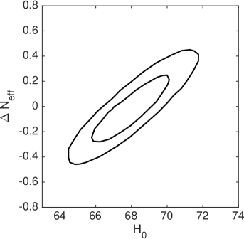
Figure 1: Marginalized posterior distributions in the $\Delta N_{\rm eff}$ and the $H_{0}$ plane [the contours correspond to the $1\sigma$ and $2\sigma$ confidence limits (C.L.)]. Here, $H_{0}$ is plotted in units of $\text{km}\ \text{s}^{-1}\text{Mpc}^{-1}$.

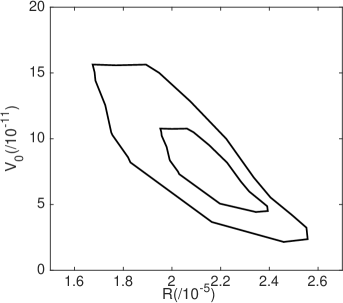
Figure 2: Favored region of the model parameter $R$ with respect to the scale of the inflation $V_{0}$ (in reduced Planck units).

For given values of the model parameters $R$ and $V_{0}$, and $N_{\rm pivot}$, we have evaluated the cosmological perturbations by using ModeChord [4] (together with CosmoMC through Multinest [24]) without assuming slow-roll conditions. Along with these parameters, we have also varied $\gamma$ which controls the amount of dark radiation produced. As usual, the Boltzmann solver CAMB [25] is used to evaluate the two-point correlation functions for temperature and polarization, and then the model parameters are estimated and the goodness of fit is determined using CosmoMC [9]. The likelihoods used here are from Planck 2018 TT+TE+EE + lowP + lensing and Planck+BICEP2/Keck array joint analysis [26]. The model parameters are then inferred from the chains of the simulation using the code in [27].

In Fig. 1, the dark radiation allowed by Planck’18 data is plotted with respect to the Hubble constant (the contours correspond to the 1$\sigma$ and 2$\sigma$ C.L.). Note that, $\Delta N_{\rm eff}$ represents the extra presence of radiation with respect to the theoretically expected $N_{\rm eff}\sim 3.046$ from the Standard Model (SM) of particle physics. We see that $\Delta N_{\rm eff}=0$ is fully consistent with the data. In Fig. 2, model parameters $R$ and $V_{0}$ are plotted against each other. We note that similar constraints of the model parameter space in the context of Kähler moduli inflation were obtained in [6].

In Fig. 3, the posterior probability distribution of the number of $e$-foldings is plotted, and the central value is found to be around $53$, which is quite close to the estimate in [14]. Finally, in Fig. 4, we have plotted the posterior probability distribution for the reheating temperature, and the most probable value is around $10^{11}$ GeV. A summary of the results for the main simulation is given in Table 1. Interestingly, the central value of $n_{s}$ here has a small shift, $n_{s}\simeq 0.9691$, as compared to the one obtained from the Planck analysis $n_{s}=0.9649$.

A rough check of our results can be done as follows. One can take the central values of the $R,V_{0}$ in Table 1 and consider the model potential (2.3) with these values for the parameters. Taking derivatives of this potential at the point in field space corresponding to the central value of $N_{\rm pivot}$ in Table 1, one finds $n^{\rm cen}_{s}=0.986$ and $r^{\rm cen}=0.0092$ (where the superscript “cen” indicates that these quantities are computed from a potential function constructed with the central values obtained from our analysis). We note that these central values are close to $n_{s}$ and $r$ obtained from our simulations (which involves a full statistical sampling over the model parameters): $r^{\rm cen}$ is very close to the value of $r$ in Table 1, while $n_{s}^{\rm cen}$ and $n_{s}$ agree approximately at the $1\sigma$ level. We take these agreements as consistency checks of our numerics.

Note that our results point to a very small amount of dark radiation. To compare with the case with sizable dark radiation, a run for a fixed value of $\Delta N_{\rm eff}=0.6$, corresponding to the theoretically well-motivated case of $\gamma=1$, was carried out (here, $N_{\rm pivot}$ was sampled as a function of the model parameters as given by (2.8), with the reheating temperature taken to be as in (2.9) with $\gamma=1$). The best-fit $\Delta\chi^{2}$ for the results in Table 1 and for the $\gamma=1$ case are, respectively, 2 and 18. This is expected because Table 1 points to the best-fit value $\Delta N_{\rm eff}=0.00041$, which corresponds to large $\gamma$. Overall, a small $\Delta N_{\rm eff}$ is preferred.

To check if there is any systematic error due to the simulation procedure adopted up to now, we have investigated fibre infation using another independently developed publicly available Markov Chain Monte Carlo (MCMC) tool named Cobaya[10]. Cobaya implements the BOBYQA algorithm [28]. It is interfaced with the Polychord nested sampler; thus, coupling ModeChord with the Cobaya becomes much easier to implement. Along with the standard Monte Carlo samples, Cobaya uses an importance-reweighting method, which makes the computation much faster and more efficient. In the end, both MCMC simulation techniques give self-consistent results, but we found it to be a good addition in the analysis, keeping in mind the sensitivity of the results quoted here. We conclude that the end results from the two independent simulations are almost independent of the MCMC sampler adopted. This indicates the robustness of our results. The results obtained using Cobaya are very consistent with the results quoted in Table 1. For the sake of completeness, we have quoted the results obtained using Cobaya in Table 3.

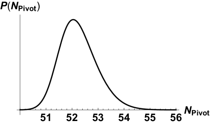
Figure 3: 1D probability distribution of the number of $e$-foldings $N_{\rm pivot}$.

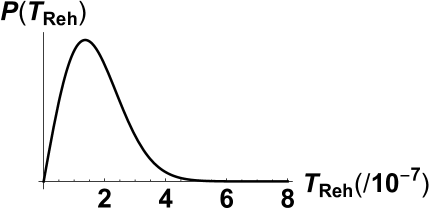
Figure 4: 1D probability distribution of the reheating temperature $T_{\rm rh}$ (in reduced Planck Units).

Parameters	Central value	$1\sigma$
$R(/10^{-5})$	2.1451	${}^{+0.0979}_{-0.0678}$
$V_{0}(/10^{-11})$	5.66	${}^{+4.51}_{-1.01}$
$\Delta N_{\rm eff}$	0.00041	${}^{+0.21}_{-0.20}$
$A_{s}(/10^{-9})$	1.300	${}^{+0.950}_{-0.350}$
$H_{0}$	68.01	${}^{+1.81}_{-3.27}$
$n_{s}$	0.9691	${}^{+0.0128}_{-0.0108}$
$r$	0.0093	${}^{+0.0005}_{-0.0006}$
$N_{\rm pivot}$	53.26	${}^{+1.58}_{-0.51}$
$T_{\rm rh}(/10^{-7})$	1.91	${}^{+0.74}_{-0.08}$

Table 1: Constraints on the model parameters and the cosmological parameters. We used the data combination Planck’18 TT+TE+EE+ low P +lensing + BKPlanck15. All dimensionful quantities are in reduced Planck units.

Parameters	Central value	$1\sigma$
$R(/10^{-5})$	$<3.05$	$--$
$V_{0}(/10^{-11})$	7.03	${}^{+3.98}_{-1.52}$
$A_{s}(/10^{-9})$	1.065	${}^{+0.840}_{-0.230}$
$H_{0}$	69.02	${}^{+1.11}_{-1.12}$
$n_{s}$	0.9830	${}^{+0.0160}_{-0.0080}$
$r$	0.0096	${}^{+0.0002}_{-0.0004}$

Table 2: Constraints on the model parameters and the cosmological parameters. We used the data combination Planck’18 TT+TE+EE+ low P +lensing + BKPlanck15. All dimensionful quantities are in reduced Planck units. In this case, $\Delta N_{\rm eff}=0.6$.

Parameters	Central value	$1\sigma$
$R(/10^{-5})$	2.13	${}^{+0.091}_{-0.051}$
$V_{0}(/10^{-11})$	5.70	${}^{+4.10}_{-0.95}$
$\Delta N_{\rm eff}$	0.0004	${}^{+0.22}_{-0.19}$
$A_{s}(/10^{-9})$	1.21	${}^{+0.881}_{-0.250}$
$H_{0}$	68.20	${}^{+1.90}_{-3.10}$
$n_{s}$	0.9701	${}^{+0.0120}_{-0.0141}$
$r$	0.0094	${}^{+0.0004}_{-0.0005}$
$N_{\rm pivot}$	53.00	${}^{+1.60}_{-0.50}$
$T_{\rm rh}(/10^{-7})$	2.00	${}^{+0.65}_{-0.15}$

Table 3: Constraints on the model parameters and the cosmological parameters using Cobaya. We used the data combination Planck’18 TT+TE+EE+ low P +lensing + BKPlanck15. All dimensionful quantities are in reduced Planck units.

4 Discussion and Conclusions

In the present work, we focused on the phenomenology of fibre inflation. We would like to begin this section by noting some issues related to the construction of the model in string compactifications. First, there is the possibility of the presence of certain $\alpha^{\prime}$ corrections [29, 30] in the effective action (which are still not completely understood) that might contribute to the positive exponential term in (2.3). One consequence of this might be that the coefficient of the positive exponential term can be pushed to higher values. In this case, our analysis would have to be redone, taking into account the appropriate range for $R$. A similar issue is the geometric instability that can arise as a result of the ultralight field in the model [31]. At this stage, it is unclear how relevant the instability is for fibre inflation, but it could have implications on the parameter space of the model. Apart from the above issues, we also note that the model is in tension with some quantum gravity conjectures which recently gained attention: the Swampland conjectures [32] and the Trans-Planckian Censorship conjecture [33]. However, the methods in the paper are general enough to be easily modified if there is better understanding of the parameter space of the model and its consistency with such conjectures.

Our results are interesting from the point of view of phenomenology. As reported in Table 1, the central value of the tensor-to-scalar ratio is $r\sim 0.00932$, which is in the observably verifiable range for the next generation of CMB B-mode surveys. More generally, the results for fibre inflation in the present article and our earlier work [6] in the context of Kähler moduli inflation show that precision cosmology can be a powerful tool to constrain string compactifications. As emphasized in Sec. 3, we have carried out our analysis using two different MCMC simulators, the results of which are consistent. This validates the robustness of the numerically computed best-fit values of the model parameters and inflationary observables quoted as our main results in Tables 1 -  3.

As future directions, it will be interesting to look for top-down constructions of string models, with the model parameters in ranges obtained from our analysis. It will also be interesting to compare with the preferred ranges from the point of view of particle physics [34]. Another phenomenologically exciting avenue is to carry out a similar analysis for closely related models, including the $\alpha$-attractor class [35].

Note added

Recently, Ref. [36] was submitted to the arXiv, which essentially addressed the same problem as this article. The methods employed and the data sets used in the two articles are different, yet, broadly, the results agree.

Ackowledgements

We would like to thank Michele Cicoli, Fernando Quevedo, L. Sriramkumar, Eleonora Di Valentino, V. Vennin, and Ivonne Zavala for discussions. A.M. would like to thank the National Taiwan University and IIT Madras for hospitality during the course of the project. M.R.G. would like to thank the Saha Institute of Nuclear Physics for hospitality during the course of the project. M.R.G. and S.B. would also like to thank the WHEPP-XVI organizers for their kind hospitality and for providing an atmosphere conducive to discussions. The work of M.R.G. is supported by the Department of Science and Technology, Government of India under Grant Agreement No. IF18-PH-228 (INSPIRE Faculty Award). S.B. is supported by the institute postdoctoral fellowship at Physical Research Laboratory, India. We also acknowledge the computation facility, 100TFLOP HPC Cluster, Vikram-100, at Physical Research Laboratory, Ahmedabad, India.

References

- [1] Y. Akrami et. al., Planck 2018 results. X. Constraints on inflation, arXiv: 1807.06211[astro-ph.CO]
- [2] K. N. Abazajian et al. [CMB-S4 Collaboration], arXiv:1610.02743 [astro-ph.CO]. T. Matsumura et al., J. Low. Temp. Phys. 176, 733 (2014) [arXiv:1311.2847 [astro-ph.IM]]. F. Finelli et al. [CORE Collaboration], arXiv:1612.08270 [astro-ph.CO].
- [3] J. Martin, C. Ringeval, JCAP 0608 (2006) 009 [arXiv: astro-ph/0605367]. J. Martin, C. Ringeval and V. Vennin, Phys. Dark Univ. 5-6, 75 (2014) [arXiv:1303.3787 [astro-ph.CO]].
- [4] M. J. Mortonson, H. V. Peiris and R. Easther, Phys. Rev. D 83 (2011) 043505 [arXiv:1007.4205].
- [5] J. Martin and C. Ringeval, Phys. Rev. D 82, 023511 (2010) [arXiv:1004.5525]. J. Martin, C. Ringeval and V. Vennin, Phys. Rev. Lett. 114, no. 8, 081303 (2015) [arXiv:1410.7958 [astro-ph.CO]]. Phys. Rev. D 93 no.10, 103532 (2016) [arXiv:1603.02606 [astro-ph.CO]]. J. Martin, C. Ringeval and R. Trotta, Phys. Rev. D 83, 063524 (2011) [arXiv:1009.4157 [astro-ph.CO]]. J. Martin, C. Ringeval, R. Trotta and V. Vennin, JCAP 1403, 039 (2014) [arXiv:1312.3529 [astro-ph.CO]].
- [6] S. Bhattacharya, K. Dutta, M. R. Gangopadhyay and A. Maharana, Phys. Rev. D 97 (2018) no.12, 123533 [arXiv:1711.04807 [astro-ph.CO]].
- [7] J. P. Conlon and F. Quevedo, JHEP 01 (2006), 146 doi:10.1088/1126-6708/2006/01/146 [arXiv:hep-th/0509012 [hep-th]].
- [8] M. Cicoli, C. P. Burgess and F. Quevedo, JCAP 0903 (2009) 013 [arXiv:0808.0691 [hep-th]].
- [9] A. Lewis and S. Bridle, Phys. Rev. D 66 (2002) 103511 [astro-ph/0205436].
- [10] J. Torrado and A. Lewis, “Cobaya: Code for Bayesian Analysis of hierarchical physical models,” [arXiv:2005.05290 [astro-ph.IM]].
- [11] B. S. Acharya, P. Kumar, K. Bobkov, G. Kane, J. Shao and S. Watson, JHEP 0806 (2008) 064 [arXiv:0804.0863 [hep-ph]]. R. Easther, R. Galvez, O. Ozsoy and S. Watson, Phys. Rev. D 89 (2014) no.2, 023522 [arXiv:1307.2453 [hep-ph]]. K. Dutta and A. Maharana, Phys. Rev. D 91 (2015) no.4, 043503 [arXiv:1409.7037 [hep-ph]]. K. Das, K. Dutta and A. Maharana, Phys. Lett. B 751, 195 (2015) [arXiv:1506.05745 [hep-ph]]. M. Cicoli, K. Dutta, A. Maharana and F. Quevedo, JCAP 1608 (2016) no.08, 006 [arXiv:1604.08512 [hep-th]]. R. Allahverdi, K. Dutta and A. Maharana, JCAP 1810 (2018) 038 [arXiv:1808.02659 [astro-ph.CO]].
- [12] M. Cicoli, J. P. Conlon and F. Quevedo, Phys. Rev. D 87 (2013) no.4, 043520 [arXiv:1208.3562 [hep-ph]]. T. Higaki and F. Takahashi, JHEP 1211 (2012) 125 [arXiv:1208.3563 [hep-ph]]. S. Angus, JHEP 1410 (2014) 184 [arXiv:1403.6473 [hep-ph]]. A. Hebecker, P. Mangat, F. Rompineve and L. T. Witkowski, JHEP 1409 (2014) 140 [arXiv:1403.6810 [hep-ph]]. M. Cicoli and F. Muia, JHEP 1512 (2015) 152 [arXiv:1511.05447 [hep-th]]. B. S. Acharya and C. Pongkitivanichkul, JHEP 1604 (2016) 009 [arXiv:1512.07907 [hep-ph]]. B. S. Acharya, M. Dhuria, D. Ghosh, A. Maharana and F. Muia, arXiv:1906.03025 [hep-th].
- [13] R. H. Cyburt et al., Rev.Mod.Phys. 88 (2016) 015004, arXiv:1505.01076 [astro-ph.CO]. N. Sasankan,M. R. Gangopadhyay,G. J. Mathews and M. Kusakabe, Phys. Rev. D 95, 083516 (2017) arXiv:1607.06858 [astro-ph.CO]. N. Sasankan,M. R. Gangopadhyay,G. J. Mathews and M. Kusakabe, IJMPE Vol. 26, No. 7 (2017) 1741007 arXiv:1706.03630 [astro-ph.CO]
- [14] M. Cicoli and G. A. Piovano, JCAP 1902 (2019) 048 [arXiv:1809.01159 [hep-th]].
- [15] P. Cabella, A. Di Marco and G. Pradisi, Phys. Rev. D 95 (2017) no.12, 123528 [arXiv:1704.03209 [astro-ph.CO]]. A. Di Marco, G. De Gasperis, G. Pradisi and P. Cabella, Phys. Rev. D 100 (2019) no.12, 123532 [arXiv:1907.06084 [astro-ph.CO]].
- [16] V. Balasubramanian, P. Berglund, J. P. Conlon, and F. Quevedo, JHEP 03 (2005) 007, [arXiv:hep-th/0502058]. J. P. Conlon, F. Quevedo and K. Suruliz, JHEP 0508 (2005) 007 [hep-th/0505076].
- [17] C. P. Burgess, M. Cicoli, S. de Alwis and F. Quevedo, JCAP 1605 (2016) no.05, 032 [arXiv:1603.06789 [hep-th]]. M. Cicoli, F. Muia and P. Shukla, JHEP 1611 (2016) 182 [arXiv:1611.04612 [hep-th]]. M. Cicoli, D. Ciupke, V. A. Diaz, V. Guidetti, F. Muia and P. Shukla, JHEP 1711 (2017) 207 [arXiv:1709.01518 [hep-th]]. M. Cicoli, I. Garcìa-Etxebarria, C. Mayrhofer, F. Quevedo, P. Shukla and R. Valandro, JHEP 1711 (2017) 134 [arXiv:1706.06128 [hep-th]].
- [18] S. B. Giddings, S. Kachru and J. Polchinski, Phys. Rev. D 66 (2002) 106006
- [19] S. Antusch, F. Cefala, S. Krippendorf, F. Muia, S. Orani and F. Quevedo, JHEP 1801 (2018) 083 [arXiv:1708.08922 [hep-th]].
- [20] B. M. Gu and R. Brandenberger, arXiv:1808.03393 [hep-th].
- [21] H. Jockers and J. Louis, Nucl. Phys. B 718 (2005) 203 [hep-th/0502059]. M. Haack, D. Krefl, D. Lust, A. Van Proeyen and M. Zagermann, JHEP 0701 (2007) 078 [hep-th/0609211].
- [22] Planck Collaboration, P. A. R. Ade et al., Astron. Astrophys. 594 (2016) A20,
- [23] A. R. Liddle and S. M. Leach, Phys. Rev. D 68, 103503 (2003) [astro-ph/0305263].
- [24] F. Feroz, M. P. Hobson and M. Bridges, Mon. Not. Roy. Astron. Soc. 398: 1601-1614,2009 arXiv:0809.3437 [astro-ph]. F. Feroz and M. P. Hobson, Mon. Not. Roy. Astron. Soc., 384, 2, 449-463 (2008) arXiv:0704.3704 [astro-ph] F. Feroz, M. P. Hobson, E. Cameron and A. N. Pettitt, arXiv:1306.2144 [astro-ph.IM].
- [25] A. Lewis, A. Challinor and A. Lasenby, Astrophys. J., 538, 473 (2000).
- [26] Keck Array, BICEP2 Collaborations: P. A. R. Ade et. al, Phys. Rev. Lett. 116, 031302 (2016). [arXiv:1510.09217]. Planck Collaboration, R. Adam et al., Astronomy and Astrophysics Volume 594, (2016) A10. P. A. R. Ade et al., Phys. Rev. Lett. 114 (2015) 101301 [arXiv:1502.00612 [astro-ph.CO]]
- [27] @manualMATLAB:R2015a, address = Natick, Massachusetts, organization = The Mathworks, Inc., title = MATLAB version 8.5.0.197613 (R2015b), year = 2015
- [28] M. J. D. Powell, “The BOBYQA algorithm for bound constrained optimisation without derivatives,” Tech. Rep. DAMTP 2009/NA06, University of Cambridge (2009).
- [29] D. Ciupke, J. Louis and A. Westphal, JHEP 1510 (2015) 094 [arXiv:1505.03092 [hep-th]].
- [30] T. W. Grimm, K. Mayer and M. Weissenbacher, JHEP 1802 (2018) 127 [arXiv:1702.08404 [hep-th]].
- [31] M. Cicoli, V. Guidetti, F. G. Pedro and G. P. Vacca, JCAP 1812 (2018) 037 d[arXiv:1807.03818 [hep-th]]
- [32] C. Vafa, [arXiv:hep-th/0509212 [hep-th]]. H. Ooguri and C. Vafa, Nucl. Phys. B 766 (2007), 21-33 doi:10.1016/j.nuclphysb.2006.10.033 [arXiv:hep-th/0605264 [hep-th]]. T. D. Brennan, F. Carta and C. Vafa, PoS TASI2017 (2017), 015 doi:10.22323/1.305.0015 [arXiv:1711.00864 [hep-th]]. E. Palti, Fortsch. Phys. 67 (2019) no.6, 1900037 doi:10.1002/prop.201900037 [arXiv:1903.06239 [hep-th]].
- [33] A. Bedroya and C. Vafa, [arXiv:1909.11063 [hep-th]]. A. Bedroya, R. Brandenberger, M. Loverde and C. Vafa, [arXiv:1909.11106 [hep-th]].
- [34] L. Aparicio, M. Cicoli, B. Dutta, S. Krippendorf, A. Maharana, F. Muia and F. Quevedo, JHEP 1505 (2015) 098 [arXiv:1502.05672 [hep-ph]]. L. Aparicio, M. Cicoli, S. Krippendorf, A. Maharana, F. Muia and F. Quevedo, JHEP 1411 (2014) 071 [arXiv:1409.1931 [hep-th]].
- [35] M. Cicoli, G. Tasinato, I. Zavala, C. P. Burgess and F. Quevedo, JCAP 1205 (2012) 039 [arXiv:1202.4580 [hep-th]]. M. Cicoli, D. Ciupke, S. de Alwis and F. Muia, JHEP 1609 (2016) 026 [arXiv:1607.01395 [hep-th]]. A. A. Starobinsky, Phys. Lett. B 91 (1980) 99 [Phys. Lett. 91B (1980) 99] ([Adv. Ser. Astrophys. Cosmol. 3 (1987) 130]). R. Kallosh and A. Linde, JCAP 1310 (2013) 033 [arXiv:1307.7938 [hep-th]]. R. Kallosh, A. Linde, D. Roest, A. Westphal and Y. Yamada, JHEP 1802 (2018) 117 [arXiv:1707.05830 [hep-th]].
- [36] M. Cicoli and E. Di Valentino, [arXiv:2004.01210 [astro-ph.CO]].