Multichannel asymmetric transmission through a dimer defect with saturable inter-site nonlinearity

Abstract

We consider the asymmetric transmission properties of a Discrete Nonlinear Schrödinger type dimer with a saturable nonlinear intersite coupling between the dimer sites, in addition to a cubic onsite nonlinearity and asymmetric linear onsite potentials. In contrast to previously studied cases with pure onsite nonlinearities, the transmission coefficient for stationary transmission is shown to be a multivalued function of the transmitted intensity, in regimes of low saturability and small or moderate transmitted intensity. The corresponding backward transfer map is analyzed analytically and numerically, and shown to have either one or three distinct solutions for saturable coupling, and zero or two solutions for the purely cubic nonlinear coupling. As saturation strength is increased, the multi-solution regimes disappear through bifurcations and the single-valued regime of the onsite model is recovered. The existence of multiple solution branches yields novel mechanisms for asymmetric left/right stationary transmission: in addition to shifts of the positions of transmission peaks, peaks for transmission in one direction may correspond to nonexistence of stationary solutions propagating in the opposite direction, at the corresponding branch and transmitted intensity. Moreover, one of these transmission channels behaves as a nearly perfect mirror for incoming signals. The linear stability of the stationary solutions is analyzed, and instabilities are typically observed, and illustrated by direct numerical simulations, in regimes with large transmission coefficient. Intersite nonlinearities are found to prevent the formation of a localized dimer mode in the instability-induced dynamics. Finally, the partial reflection and transmission of a Gaussian excitation is studied, and the asymmetric transmission properties are compared to previously studied onsite models.

I Introduction

During the last decade, there has been a major interest in using nonlinearity for achieving non-reciprocal transmission, aiming at designing efficient wave diodes in particular with applications within the optical domain. The basic idea, that transmission between two waveguides with intensity-dependent (Kerr) refractive index and different propagation constants becomes asymmetric in the nonlinear regime, was probably first put forward by Trillo and Wabnitz TW86 . A similar mechanism was later analyzed for a different setup by Lepri and Casati 11 ; lepri , who considered the nonreciprocal transmission through a layered photonic (or phononic) system, with a small central segment of nonlinear, nonmirror symmetric layers embedded in an infinite linear lattice. In both cases, the systems were modeled using a discrete nonlinear Schrödinger (DNLS) equation with cubic on-site nonlinearity, with particular focus on the case with two nonlinear sites (DNLS dimer) which can be solved exactly. As is well known DLS86 ; WS ; btm , stationary transmission through DNLS chains with on-site nonlinearity generically exhibits multistability and hysteresis effects when using input intensity $|R_{0}|^{2}$ as independent parameter, while the existence of a backward transfer map guarantees that the stationary transmission coefficient is a single-valued function of the output intensity $|T|^{2}$ .

Later, in the context of asymmetric transmission of signals through non-linear asymmetric dimer layers, it was shown that multistability could be enhanced by weak saturation of the (cubic) on-site nonlinearity; this favors the nonreciprocal transmission and also yields opposite effects of the rectifying action for short/long wavelength signals assuncao ; Erik . A similar study was carried out for saturable nonlinear oligomer DNLS segments ($N=1,2,3$) embedded in a linear Schrödinger chain jd . Other relevant works concern the asymmetric wave transmission through oligomers with cubic-quintic on-site nonlinearity wasay18 , and the enhancement of the non-reciprocal transmission under saturable cubic-quintic nonlinear responses for dimers wasay3 . A cubic on-site nonlinearity was also shown to yield non-reciprocal transmission if combined with an asymmetric geometric shape of the nonlinear part LiRen , and moreover, for a system with two nonlinear sites separated by a number of linear sites, the transmission was shown to be generically asymmetric unless certain resonance conditions were fulfilled RenPRB (analogous resonance conditions were also obtained for the continuous Schrödinger equation with nonlinear $\delta$-function scatterers RenPRB ; RenPRE )

A common feature of the above mentioned earlier works is, that the nonlinearity (cubic, cubic-quintic or saturable) resided only in the on-site terms, which simplifies the analytical as well as the numerical treatment due to the existence of a unique backward transfer map, which thus never yields more than one solution for a given output $|T|$. However, although on-site nonlinearities typically dominate in most physical applications of DNLS lattices, there are certain situations where the additional effects of inter-site nonlinearities may be important, e.g., for optical waveguides embedded in a nonlinear medium Oster03 , Bose-Einstein condensates in optical lattices ST03 (dipolar condensates in particular Serbia ; Chile ), or, more generally, when the DNLS equation is considered as a rotating-wave type approximation of anharmonically coupled oscillators MJ06 , or as a tight-binding approximation of the nonlinear Schrödinger equation with spatial periodicity in both the linear potential and nonlinearity coefficient Abd08 . It is thus also of interest to investigate, whether the presence of a non-negligible inter-site nonlinearity in the central segment may have any major qualitative effects on the non-reciprocal wave transmission. A first step in this direction was taken in wasay2 , where transmission through an asymmetric DNLS dimer with cubic on-site as well as inter-site nonlinearity was studied for a special situation, assuming a particular relation between the complex amplitudes of the two dimer sites, that allowed the derivation of a unique backward transfer map and thus a unique solution for a given $|T|$. However, as we will show in the present work, this is not the case for the generic situation in presence of inter-site nonlinearities.

In this work, we generalize the model introduced in wasay2 to have a saturable inter-site nonlinearity between the two dimer sites, leaving the on-site nonlinearity cubic. As we will see, due to the absence of a unique backward transfer map, a small inter-site saturability typically yields more than one solution in the regime of small $|T|$. These solutions are distinguished by their different relative phases between the dimer sites, and may be obtained numerically by solving an additional equation for this phase difference. Most importantly, the general distinctive feature of this work in view of all previous works is that we will present the scenario of how a gradual transition from the non-saturated to saturated case takes place, i.e., to analyse in detail how the saturated inter-site case connects to the non-saturated inter-site case.

Although we consider here a specific form of saturable inter-site nonlinearities, appropriate e.g. for photvoltaic-photorefractive materials Valley94 , the method that we present should be applicable for transmission through generic inter-site nonlinear dimer segments. Notably, a somewhat different form of saturable nonlinear coupling within a dimer was recently proposed Hadad17 and implemented through an electric circuit ladder Hadad18 .

The outline of this paper is as follows. In Sec. II we introduce the dynamical model and set up the corresponding stationary transmission problem. We derive the corresponding backward transfer map, point out the reason for its general non-uniqueness, and analyze its solutions analytically in some limiting cases. In Sec. III we investigate in more detail, by numerical means, the transitions between regimes with two, three, or one distinct solutions of the backward transfer map, for increasing saturation strength. Results for the multi-channel stationary transmission coefficients as a function of wave number and transmitted intensity, for given parameter values and varying saturation strength, are reported in Sec. IV. The asymmetric stationary transmission properties are investigated in Sec. V, where also the rectification factor is calculated in various regimes of saturability for the different solution branches. Section VI reports the linear stability analysis of the different branches of stationary scattering solutions, with illustrations of instability-induced dynamics. In Sec. VII we perform dynamical simulations with Gaussian wavepackets and discuss the transmission and rectification properties. Concluding remarks are made in Sec. VIII, and some results for different parameter values than those used in the main paper are shown in Appendix.

II Model

We introduce the dynamical equation of the model as follows,

$$i\frac{dA_{n}}{dt}\!=\!V_{n}A_{n}\!-\!C\!\left(A_{n+1}\!+\!A_{n-1}\right)\!+\!\gamma_{n}|A_{n}|^{2}A_{n}\!+\!\left(\!\frac{\epsilon_{n}|A_{n+1}|^{2}}{1\!+\!\beta|A_{n+1}|^{2}|A_{n}|^{2}}\!+\!\frac{\epsilon_{n-1}|A_{n-1}|^{2}}{1\!+\!\beta|A_{n-1}|^{2}|A_{n}|^{2}}\!\right)\!A_{n}.$$ (1)

In Eq. (1), $n$ is the lattice site counter, $A_{n}$ is the amplitude at site $n$, and $V_{n}$ is the linear on-site energy of each site inside the one-dimensional lattice. The parameter $\gamma_{n}$ determines the strength of the local nonlinearity, which we take to have a standard cubic (Kerr) form, while $\epsilon_{n}$ represents the nonlocal (inter-site) saturable nonlinearity. We saturate only the inter-site nonlinearity as the effect of saturating the on-site cubic nonlinearity has been addressed in earlier work jd ; assuncao ; wasay3 ; Erik . $\beta$ is the saturation parameter; in the unsaturated limit $\beta=0$ we recover the DNLS model with cubic inter-site nonlinearity studied in wasay2 (relevant e.g. for dipolar Bose-Einstein condensates Chile ), while in the strongly saturated limit $\beta\rightarrow\infty$ the coupling becomes governed only by the linear coupling constant $C$, and the model reduces to the standard cubic on-site DNLS model 11 ; lepri . Like the standard DNLS model EJ03 , the system is Hamiltonian, with the saturable inter-site terms arising from additional terms $\frac{\epsilon_{n}}{\beta}\ln\left(1+\beta|A_{n}|^{2}|A_{n+1}|^{2}\right)$ in the Hamiltonian. Without loss of generality, the parameter $C$ will be chosen to be unity. Focusing our attention on a dimer situated at lattice sites 1 and 2 with nonlinear inter-site interactions only between the two dimer sites, the site dependent parameters $\gamma$ and $V$ have non-zero contributions only in the region $1\leq n\leq 2$, and $\epsilon$ only for $n=1$. This means that waves can propagate freely outside the dimer.

The set of dynamical equations (1) has stationary solutions of the form $A_{n}(t)=A_{n}e^{-i\omega t}$. When a signal (incoming or outgoing wave) is away from the dimer, the system is linear, and these solutions satisfy the dispersion relation $\omega=-2$cos$k$, with $k$ being the wave vector of some specific harmonic component of the wave and $0\leq k\leq\pi$. These solutions render Eq. (1) stationary. The resulting stationary equation can be written in the form of a backward-map analogous to 11 ; btm ,

$$A_{n-1}=-A_{n+1}+\left(V_{n}-\omega+\gamma_{n}|A_{n}|^{2}+\frac{\epsilon_{n}|A_{n+1}|^{2}}{1+\beta|A_{n+1}|^{2}|A_{n}|^{2}}+\frac{\epsilon_{n-1}|A_{n-1}|^{2}}{1+\beta|A_{n-1}|^{2}|A_{n}|^{2}}\right)A_{n}.$$ (2)

In the absence of inter-site nonlinearities ($\epsilon_{n}\equiv 0$), this relation allows one to immediately construct the amplitudes by a backward iteration, assuming that the solution is known at $n\rightarrow\infty$. By contrast, with nonzero $\epsilon_{1}$ an additional relation between the complex amplitudes $A_{1}$ and $A_{2}$ at the nonlinear dimer sites is needed. We will focus on the scattering properties of plane wave solutions of the following form,

$$A_{n}=\Bigg{\{}\begin{array}[]{c}R_{0}e^{ikn}+Re^{-ikn}\qquad n\leq 1\\ Te^{ikn}~{}~{}\qquad\qquad\qquad n\geq 2\\ \end{array},$$ (5)

where $R_{0}$, $R$ and $T$ are the amplitudes of incoming, reflected and transmitted wave, respectively. Applying the ansatz in Eq. (5) site-by-site, we get at site $n=0$,

$$A_{0}=R_{0}+R,$$ (6)

and at site $n=1$,

$$A_{1}=R_{0}e^{ik}+Re^{-ik}.$$ (7)

With $A_{0}$ and $A_{1}$, the amplitudes of the reflected and incident waves can be computed as

$$R=\frac{A_{0}e^{ik}-A_{1}}{e^{ik}-e^{-ik}},$$ (8)

and

$$R_{0}=\frac{A_{0}e^{-ik}-A_{1}}{e^{-ik}-e^{ik}}.$$ (9)

We can rewrite the backward map (2) for the dimer ($n=2$), with the inter-site nonlinear interactions considered only between the two dimer sites, as

$$A_{1}=-A_{3}+\left(V_{2}-\omega+\gamma_{2}|A_{2}|^{2}+\frac{\epsilon_{1}|A_{1}|^{2}}{1+\beta|A_{1}|^{2}|A_{2}|^{2}}\right)A_{2}.$$ (10)

With Eq. (5), the wave amplitudes at the dimer interface for the outgoing, right-propagating waves ($k>0$) is $A_{2}=Te^{2ik}$ and $A_{3}=Te^{3ik}$. In addition, we may obtain an expression for $|A_{1}|^{2}$ from the general current conservation law for stationary solutions,

$$\textmd{Im}[A_{n}^{\ast}A_{n+1}]=|T|^{2}\sin k,$$ (11)

for all $n$. Without loss of generality, we may choose the arbitrary overall phase such that the amplitude $A_{1}$ at site 1 is real. From (11) with $n=1$ and (5) with $n=2$ it then follows straightforwardly that $A_{1}\textmd{Im}(Te^{2ik})=|T|^{2}\sin k$, i.e.,

$$|A_{1}|^{2}=\frac{|T|^{4}\textmd{sin}^{2}k}{[\textmd{Im}(Te^{2ik})]^{2}}.$$ (12)

The fact that $T$ is not real in general then leads to the following relation,

$$|A_{1}|^{2}=\frac{|T|^{2}\sin^{2}k}{[\sin(2k+\varphi)]^{2}},$$ (13)

where $\varphi=\textmd{arg}(T)$. Thus, Eq. (10) becomes

$$A_{1}=-Te^{3ik}+\left(V_{2}-\omega+\gamma_{2}|T|^{2}+\frac{\epsilon_{1}|T|^{2}\textmd{sin}^{2}k}{\left[\textmd{sin}(2k+\textmd{arg}(T))\right]^{2}+\beta|T|^{4}\textmd{sin}^{2}k}\right)Te^{2ik},$$ (14)

which can be re-written as

$$A_{1}=Te^{2ik}(\delta_{2}-e^{ik}),$$ (15)

with $\delta_{2}=V_{2}-\omega+\gamma_{2}|T|^{2}+\frac{\epsilon_{1}|T|^{2}\textmd{sin}^{2}k}{\left[\textmd{sin}(2k+\textmd{arg}(T))\right]^{2}+\beta|T|^{4}\textmd{sin}^{2}k}$.

Now in a similar way, for $n=1$ with the nonlinear inter-site interactions only between the two dimer sites, from Eq.(2) we get

$$A_{0}=-A_{2}+\left(V_{1}-\omega+\gamma_{1}|A_{1}|^{2}+\frac{\epsilon_{1}|A_{2}|^{2}}{1+\beta|A_{1}|^{2}|A_{2}|^{2}}\right)A_{1},$$ (16)

which together with Eq.(15) leads to

$$A_{0}=-Te^{2ik}+\left(V_{1}-\omega+\gamma_{1}|T|^{2}|\delta_{2}-e^{ik}|^{2}+\frac{\epsilon_{1}|T|^{2}}{1+\beta|T|^{4}|\delta_{2}-e^{ik}|^{2}}\right)Te^{2ik}(\delta_{2}-e^{ik}),$$ (17)

which can be rewritten as

$$A_{0}=Te^{2ik}\left[\delta_{1}(\delta_{2}-e^{ik})-1\right],$$ (18)

with $\delta_{1}=V_{1}-\omega+\gamma_{1}|T|^{2}|\delta_{2}-e^{ik}|^{2}+\frac{\epsilon_{1}|T|^{2}}{1+\beta|T|^{4}|\delta_{2}-e^{ik}|^{2}}$.

This implies that the transmission coefficient $t(k,|T|^{2};\arg(T))$ can now be computed by using Eq. (18) and Eq. (15) in Eq. (9). The result is

$$t(k,|T|^{2};\arg(T))=\frac{|T|^{2}}{|R_{0}|^{2}}=\left|\frac{e^{-ik}-e^{ik}}{(\delta_{2}-e^{ik})(\delta_{1}-e^{ik})-1}\right|^{2}.$$ (19)

For the left-propagating waves (with $k<0$), a similar computation yields the transmission coefficients, i.e., we only need to exchange the subscripts 1 & 2.

Note that, in contrast to previously studied DNLS-type transmission problems (e.g., 11 ; lepri ; DLS86 ; WS ; btm ; assuncao ; Erik ; jd ; wasay18 ; wasay3 ; LiRen ; RenPRB ), Eq. (19) does not necessarily determine the transmission coefficient for a plane wave of wave vector $k$ as a unique function of the transmitted intensity $|T|^{2}$, since in presence of intersite nonlinearities, there may be multiple solution branches $i$ corresponding to the same $|T|^{2}$ but with different phases $\varphi_{i}\equiv\arg(T)$. Since Eq. (14) was obtained by assuming $A_{1}$ real, the interpretation of the quantity “$\arg(T)$” is an additional phase shift between the two dimer sites 1 and 2, due to the internal properties of the dimer. The computation of this additional phase factor $\arg(T)$ is nontrivial. Imposing the ”reality” assumption on $A_{1}$ by putting the imaginary part of the right-hand side of Eq. (14) to zero, leads to the following equation,

$$\frac{\sin\left[3k+\arg(T)\right]}{\sin\left[2k+\arg(T)\right]}=V_{2}-\omega+\gamma_{2}|T|^{2}+\frac{\epsilon_{1}|T|^{2}\sin^{2}k}{\left[\sin(2k+\arg(T))\right]^{2}+\beta|T|^{4}\sin^{2}k}.$$ (20)

Solving Eq.(20) analytically for $\arg(T)=\varphi_{i}(|T|,k)$ is nontrivial in the general case, but we may immediately note that adding any multiple of $\pi$ to a solution gives another solution, so we may restrict to the interval $0\leq\varphi<\pi$ (adding $\pi$ just switches an overall sign). For the case with pure on-site nonlinearity ($\epsilon_{1}=0$), we recover the unique solution

$$\varphi_{\epsilon_{1}=0}(|T|,k)=-2k+\arctan\left[\frac{\sin k}{V_{2}+\cos k+\gamma_{2}|T|^{2}}\right].$$ (21)

Note that in the linear limit ($|T|\to 0$) and non-scattering case ($V_{2}=0$), Eq. (21) yields $\arg(T)=-k$ (due to the choice of origin in (5)).

With unsaturated inter-site nonlinearity ($\epsilon_{1}\neq 0$ but $\beta=0$), Eq. (20) can be written as a quadratic equation for $y\equiv\sin^{2}(2k+\varphi)$:

$$y^{2}(e^{2}+\sin^{2}k)+y(2e\epsilon_{1}|T|^{2}-1)\sin^{2}k+\epsilon_{1}^{2}|T|^{4}\sin^{4}k=0,$$ (22)

where $e\equiv V_{2}+\cos k+\gamma_{2}|T|^{2}$. Thus, it is clear from (22) that for unsaturated inter-site nonlinearities there are generally two distinct solutions for small $|T|$, and no solutions for large $|T|$. For small $|T|$ we may express the solutions to $O(|T|^{4})$ as

$$\varphi_{1}\simeq-2k+\arctan\left[\frac{\sin k}{V_{2}+\cos k}\left\{1-\frac{\gamma_{2}+\epsilon_{1}[(V_{2}+\cos k)^{2}+\sin^{2}k]}{V_{2}+\cos k}|T|^{2}\right\}\right],$$ (23)

and

$$\varphi_{2}\simeq-2k,$$ (24)

respectively. Thus we note that the solution $\varphi_{1}$ in (23) coincides with the small-$|T|$ limit of the pure on-site solution (21) when $\epsilon_{1}\rightarrow 0$, while the solution $\varphi_{2}$ in (24) yields a new possible transmission channel not existing for pure on-site nonlinearity (the existence of this additional channel was suppressed in wasay2 due to the choice of a specific relation between the complex amplitudes of the dimer sites).

For the general case with saturable inter-site nonlinearity ($\beta\neq 0$), Eq. (20) instead becomes a cubic equation for $y$ ($0\leq y\leq 1$),

$$(y+\beta|T|^{4}\sin^{2}k)^{2}(1-y)\sin^{2}k=y\left[e(y+\beta|T|^{4}\sin^{2}k)+\epsilon_{1}|T|^{2}\sin^{2}k\right]^{2}.$$ (25)

Thus, depending on the parameter values, there are either one or three distinct solutions $\varphi_{i}$, corresponding to different possible transmission channels. By analyzing the coefficients in (25), we find that in the limit of small $|T|$ there is a transition at $\beta/\epsilon_{1}^{2}=1/4$, so that for $\beta/\epsilon_{1}^{2}>1/4$ there is only one real and positive solution for $y$, corresponding to the phase factor $\varphi_{1}$ in (23) for the unsaturated case. On the other hand, for $\beta/\epsilon_{1}^{2}<1/4$ two additional solutions appear, both originating from the solution $\varphi_{2}$ in (24) for the unsaturated case, with corrections of order $|T|^{4}$ and higher. Below, the value $\beta/\epsilon_{1}^{2}=1/4$ will be taken as indicating the transition between regimes of “low saturation” and “medium saturation”.

Moreover, in the limit of large $|T|$, $y=0$ is the only real solution, thus yielding a single channel with phase factor $\varphi_{2}$ given by (24). Note that this agrees also with the large-$|T|$ limit of the pure on-site solution (21), as it should since the coupling becomes effectively linear due to strong saturation. For general nonzero $|T|$, the phase factor $\varphi_{i}(|T|,k)$ is computed numerically, and we will illustrate the typical scenario for different regimes of saturability in the following section. As we will see, there are significant regimes with three distinct channels for small and intermediate values of $|T|$ when $\beta$ is not too large.

III Multiple transmission channels

As described above, one of our goals is to investigate how the saturated case connects to the non-saturated case, which hinges on the detailed investigation of scenarios occurring at different levels of saturation. The analysis is thus divided into three distinct saturation regimes with carefully chosen representative saturation values. To be specific, we fix the value of $\epsilon_{1}$ to $\epsilon_{1}=0.5$, consider an “ultra-low saturation” regime for $\beta=0.01$ (i.e., $\beta/\epsilon_{1}^{2}=0.04\ll 1/4$), a low saturation regime for $\beta=0.05$ (i.e., $\beta/\epsilon_{1}^{2}=0.2<1/4$), and a medium saturation regime $\beta=0.5$ (i.e., $\beta/\epsilon_{1}^{2}=2>1/4$) (the regime of stronger saturations is less interesting since it essentially reproduces well known results for pure on-site nonlinearity 11 ; lepri ). Unless otherwise noted, we will also fix the on-site nonlinearity strength on the dimer symmetric as $\gamma_{1}=\gamma_{2}=1$, and express the asymmetric on-site potential as $V_{1,2}=V^{(0)}(1\pm\varepsilon_{V})$, with specifically chosen $V^{(0)}=-2.50$ and $\varepsilon_{V}=0.05$ (some results for different values of $\varepsilon_{V},V^{(0)}$ are discussed in Appendix A).

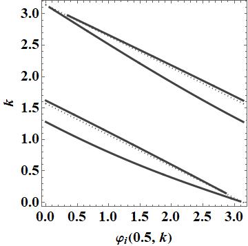
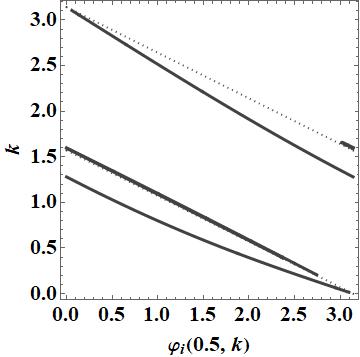
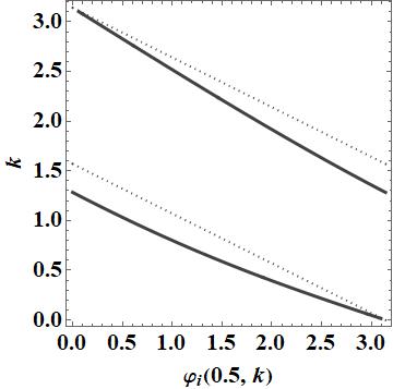
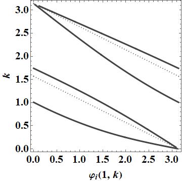
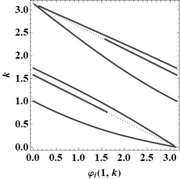
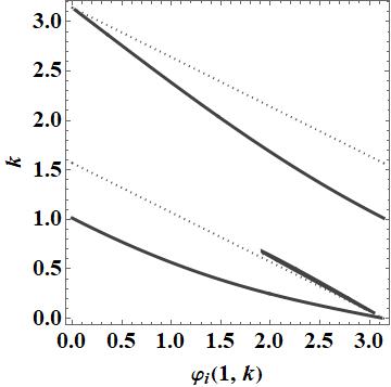
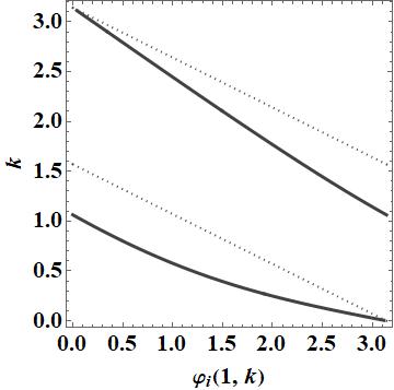
Figure 1: Contour plot of solutions of Eq.(20) as a function of $k$ and $\arg(T)=\varphi_{i}(|T|,k)$ for $V_{2}=-2.3750$, $\gamma_{2}=1$ and $\epsilon_{1}=0.5$. Upper row: $|T|=0.5$; lower row: $|T|=1$. Columns from left to right: $\beta=0$, $\beta=0.01$, $\beta=0.05$, $\beta=0.5$.

The solutions to Eq. (20) for two distinct nonzero $|T|$ values ($|T|$=0.5 and $|T|$=1) in the unsaturated and the three saturation regimes are illustrated in Fig. 1 for $0\leq k\leq\pi$ versus $0\leq\varphi_{i}(|T|,k)\leq\pi$. The ”dotted” lines in these figures represent the singularity in the left-hand side of (20) at $y=0$ ($\varphi=-2k\mod\pi$), which lies very close to the actual solution for some cases. In Fig. 2, the corresponding solutions ($\varphi_{i}(|T|,k)$) are presented as a function of $|T|$ for various (fixed) values of $k$.

Firstly, for the non-saturated case ($\beta=0$, left columns in Figs. 1-2), as predicted from (22) there is a two-solution regime which exists for all $k$ for small $|T|$, and no valid solutions for higher $|T|$ above a certain cut-off, which differs slightly for different $k$. For the chosen set of parameter values, in the case of relatively small $k\leq 1.4$ this cut-off value is approximately $|T|=1.2$, and slightly increases for larger $k$ values, i.e., for $2.8\leq k\leq\pi$, the cut-off is at $|T|=1.8$ approximately. Thus, there are either two or zero transmission channels in the case of zero saturation.

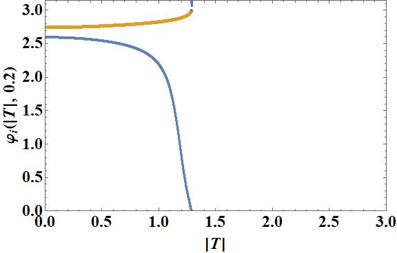
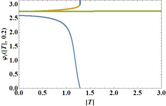
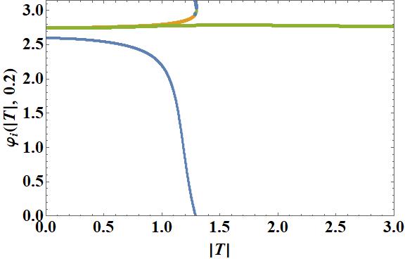
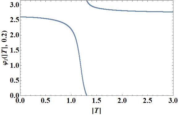
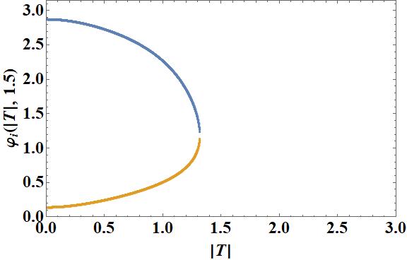
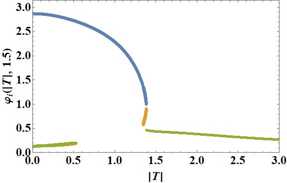
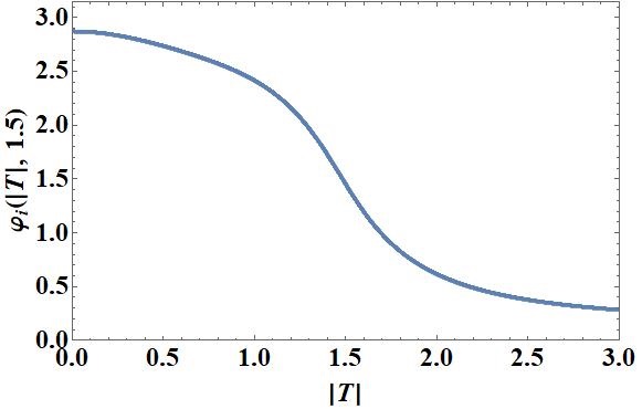
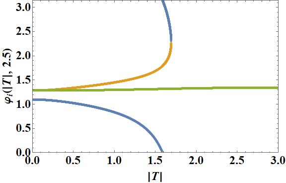
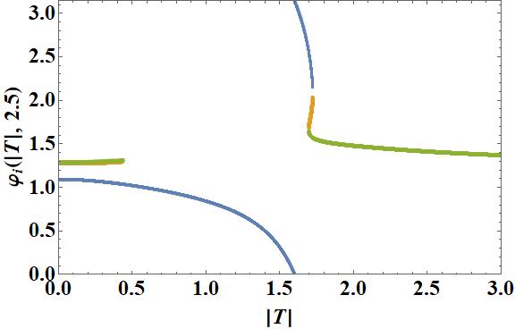
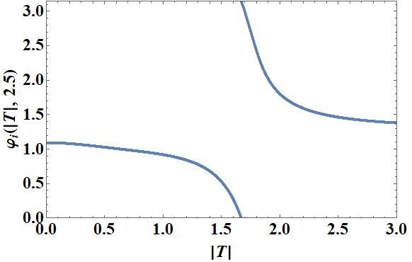
Figure 2: Plots of $\varphi_{i}(|T|,k)$ as a function of $|T|$ with three fixed values of $k$: $k=0.2$ (upper row), $k=1.5$ (middle row), $k=2.5$ (bottom row). Columns from left to right: unsaturated case ($\beta=0$), ultra-low ($\beta=0.01$), low ($\beta=0.05$), and medium saturation ($\beta=0.5$) strengths. All other parameter values as before. Blue, orange and green curves correspond to the first, second and third solution branch, respectively.

As soon as we switch from the unsaturated to the ultra-low saturation (second column in Figs. 1-2), a third solution immediately appears in the small-$|T|$ solution regime, as predicted from (25). Note that this additional solution (green curve in Fig. 2) as expected almost coincides with the “singularity line” $\varphi=-2k\mod\pi$ in Fig. 1. Above a certain cut-off depending upon $k$ (which is essentially the same as for the unsaturated case), only this new third solution persists throughout the parameter space. So there is either a three-solution regime (for small $|T|$) or a single-solution regime for higher $|T|$.

For the case of low saturations ($\beta=0.05$, third column in Figs. 1-2), the three-solution regime as predicted always persists for small $|T|$ (orange and green branches in Fig. 2 almost coincide) and also for small $k$ (the apparent gap close to $k=0$ in Fig. 1 is due to graphics limitations). However, for slightly larger $k$ ($k>0.6$), the scenario is different as compared to the ultra-low case: the three-solution regime at small $|T|$ is interrupted by a single-solution regime (blue curve only in Fig.  2) for some interval of $|T|$, and then there is a second (small) three-solution regime which exists upto a cut-off as in the ultra-low case. For all higher $|T|$, there is a single solution (the third solution, green curve in Fig.  2). Note however that the single-solution regime sandwiched between the two three-solution regimes does not belong to the ’third solution branch’, but rather it belongs to the ’first solution branch’.

Finally, in the medium saturation range ($\beta=0.5$, right column in Figs. 1-2)), the multi-solutions are entirely suppressed leaving behind only a single-solution regime for all $k$ and $|T|$.

Also, it is to be noted (see Appendix A) that the stretch of intensities that exhibit the multi-channel regime strongly depends on the energy at site 2, represented by the parameter $V_{2}$. For a smaller $V_{2}$ the multi-channel regime persists for a longer stretch of intensities (i.e., the cut-off is higher) and vice versa.

IV Effects of saturation on multi-channel transmission

In this section, we present in Fig.  3 the transmission scenario via density plots of the transmission coefficient $t(k,|T|^{2})$ from Eq. (19), for the parameter values corresponding to the different saturation regimes discussed above. The first, second and third transmission channels correspond to blue, orange and green curves from Fig. 2, respectively. The results for the two transmission channels in the unsaturated case ($\beta=0$) are visually identical to those of the first and second channels for the ultra-low saturation ($\beta=0.01$), and thus we do not show these figures below.

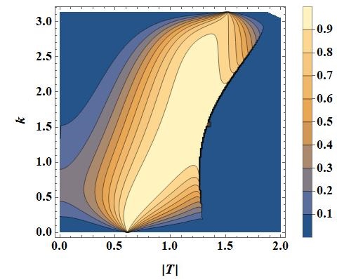
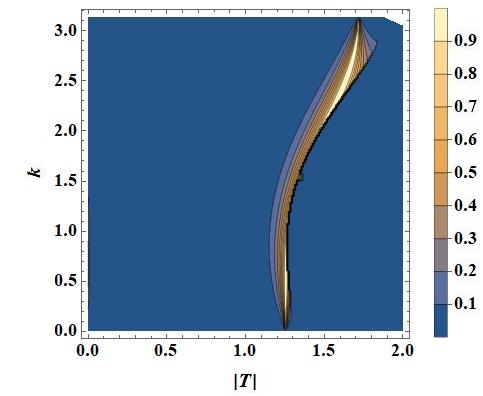
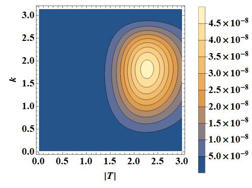
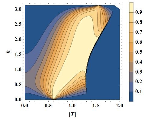
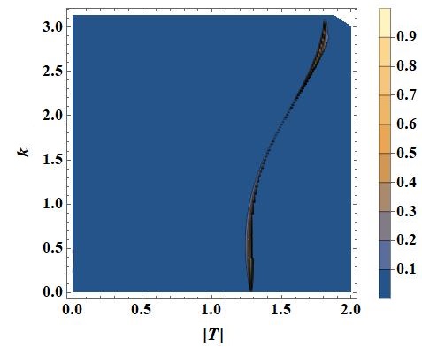
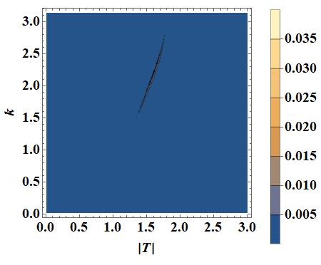
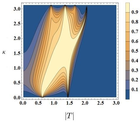
Figure 3: Color plots of transmission coefficient as a function of $k$ and $|T|$ for the three different saturation regimes. Upper row: $\beta=0.01$; middle row: $\beta=0.05$; lower row: $\beta=0.5$. Left, middle and right panels in two upper rows correspond to the 1st, 2nd and 3rd transmission channel, respectively. In all figures, $\epsilon_{1}=0.5$, $\varepsilon_{V}=0.05$, $V^{(0)}=-2.5$, and $\gamma_{1,2}=1$.

Ultra Low Saturation Regime, $\beta=0.01$

From the upper row in Fig. 3, we see that the major regimes of good transmission occur along the first channel, and that transmission along the third channel is essentially negligible. Note however that there is a narrow peak with close to perfect transmission also along the second channel, most apparent around $k=0.2$ and $k=2.5$. This second peak appears also for pure on-site nonlinearities 11 ; wasay18 ; what is important to note here is thus that with inter-site nonlinearity (unsaturated or with ultra-low saturation), the second transmission peak moves over to the second branch of solution, and thus there is only one peak in each of the two first channels.

Low Saturation Regime, $\beta=0.05$

Here, we see from the second row of Fig. 3 that the transmission along the first channel is essentially the same as for smaller saturation, but that of the second channel narrows down as the existence region for the corresponding solution shrinks, as discussed above. Note that when $\beta=0.05$ there are two distinct three-solution regimes for $k>0.6$ (see Fig. 2), but the transmssion along the second and third channels is always negligible in the small-$|T|$ region. Note also that since the third solution now connects to the second solution when $k>0.6$, it also picks up some noticeable, but still small, transmission close to the connection point (seen for $1.4\lesssim|T|\lesssim 1.8$ in Fig. 3).

Medium Saturation Regime, $\beta=0.5$

As discussed above, in the medium saturation regime only single solutions persist throughout the parameter space. The transmission coefficient shown in the lowest part of Fig.  3 is qualitatively similar to analogous plots for the pure on-site nonlinearity case 11 ; wasay18 : two separate transmission peaks for small $k$ which merge to a single, broad peak around $k=\pi/2$, and then split up again, eventually yielding four distinct peaks close to $k=\pi$. Note also that although a propagating solution exists for arbitrarily large $|T|$ and all $k$, the transmission coefficient is essentially negligible for $|T|\gtrsim 2.1$.

V Asymmetric multi-channel transmission

Having identified regimes of multi-solutions, we now consider the possibility for multi-channel asymmetric transmission due to the presence of a small nonzero asymmetry between on-site energies. To determine the efficiency of nonreciprocal transmission, i.e., transmission at diode-like modes, we define the rectifying factor $\mathcal{R}$ as 11

$$\mathcal{R}=\frac{t(k,|T|^{2})-t(-k,|T|^{2})}{t(k,|T|^{2})+t(-k,|T|^{2})},$$ (26)

where $-1\leq\mathcal{R}\leq+1$. A perfect diode-like transmission occurs at $\mathcal{R}=\pm 1$. In Fig. 4 we present the results of the rectifying factor along the different transmission channels for the three different saturability regimes (as in previous section, the results for the unsaturated case is visually identical to those of the first two channels for the ultra-low saturation, and thus not shown).

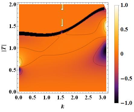
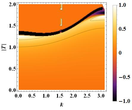
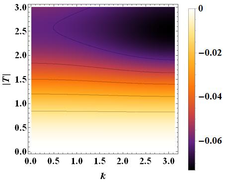
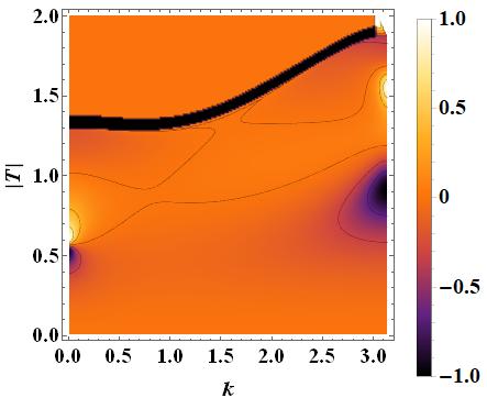
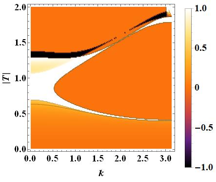
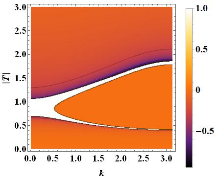
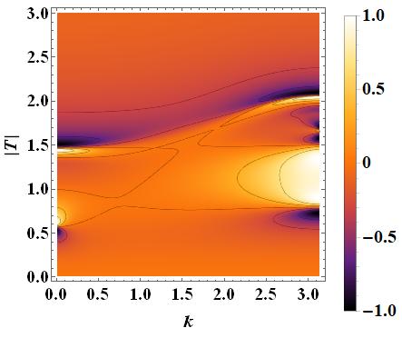
Figure 4: Color plots of rectifying action for $\beta=0.01$ (upper row), $\beta=0.05$ (middle row) and $\beta=0.5$ (lower row). In two upper rows, the three panels from left to right correspond to the first, second and third solution, respectively. Site dependent parameter strengths $V^{(0)}=-2.5$, $\varepsilon_{V}=0.05$, $\epsilon_{1}=0.5$, $\gamma_{1,2}=1$. In two upper rows, regimes where the channel transmits only right-propagating (left-propagating) modes are coded white (black), while regimes where the channel has no solutions for any propagation direction are coded orange.

The transmission scenario is presented in more detail below via plots of the transmission coefficient $t(k,|T|^{2})$ in Eq. (19) as a function of transmitted intensity $|T|^{2}$ for the case of ultra-low saturation ($\beta=0.01$), low saturation ($\beta=0.05$) and medium saturation ($\beta=0.5$) in Fig. 5, Fig. 6 and Fig. 7, respectively. Note that the blue curves in Figs. 5 - 7 correspond to the right-propagating case ($k>0$), while the red dotted curves represent the left-propagation ($k<0$), both plotted in their respective existence regimes. Note also that the first, second and third solution branches in these figures correspond to blue, orange and green curves from Fig. 2, respectively.

Ultra-Low Saturation, $\beta=0.01$

For the first transmission channel, we see from upper left Fig. 4 that there are essentially two regimes with considerable rectification action that also correspond to large transmission coefficients according to Fig. 3: a regime for small $k$ and $T\approx 0.5$, and another regime for large $k$ around $T\approx 1$. As seen in upper and lower left Fig. 5, these regimes originate in shifts of large-amplitude transmission peaks, and are analogous to large-rectification regimes existing for pure on-site nonlinearities 11 ; wasay18 . On the other hand, in the regime of intermediate $k$ where transmission peaks are broad, transmission is close to symmetric as seen in middle left Fig. 5. Moreover, the black band with $\mathcal{R}=-1$ in upper left Fig. 4 for $1.3\lesssim|T|\lesssim 1.9$ arises since the existence regime for the first transmission channel is always smaller for the right-propagating wave than for the left-propagating for the corresponding set of parameter values (see left vertical panel in Fig. 5).

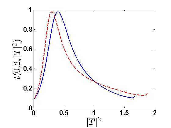
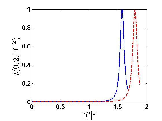
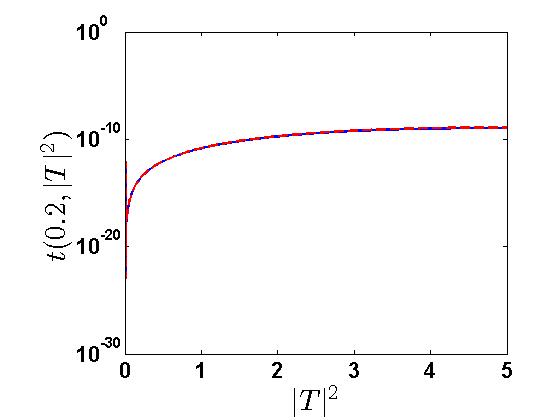
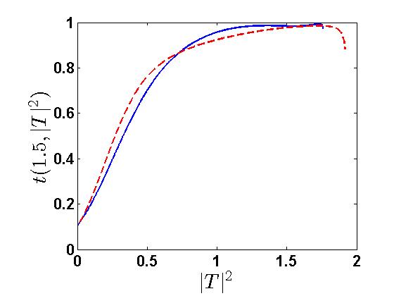
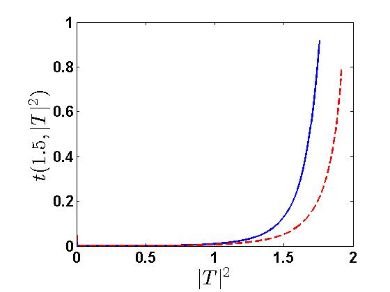
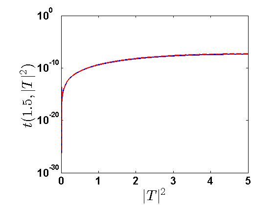
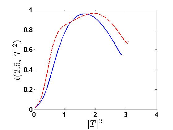
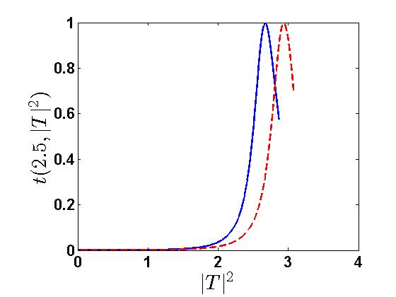
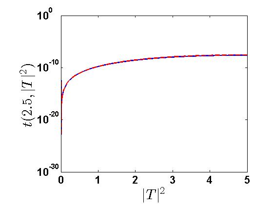
Figure 5: Transmission coefficient $t(k,|T|^{2})$ as a function of $|T|^{2}$ for the ultra-low saturated case $\beta=0.01$ for fixed $k$ values, from top to bottom $k=0.2,1.5,2.5$. Left, middle and right vertical panels correspond to first, second and third solution branches, respectively. All parameter values as before.

For the second transmission channel, the most interesting effect is the shift of the narrow transmission peak with close to perfect transmission, leading to the bright band with $\mathcal{R}$ close to 1 for $1.1\lesssim|T|\lesssim 1.8$ in upper middle Fig. 4. This is seen more explicitly in the middle vertical panel of Fig. 5. Note also the small regime with $\mathcal{R}$ close to -1 for $k$ close to $\pi$ and $1.8\lesssim|T|\lesssim 1.9$, corresponding to the peak of almost perfect left-propagating transmission appearing while the right-propagating transmission is declining. As the existence regimes for the first and second solutions are identical in the regime of ultra-low saturability, the black band with $\mathcal{R}=-1$ for the second solution in upper middle Fig. 4 will be the same as that for the first solution.

Finally, as seen in upper right Fig. 3 the transmission along the third channel (corresponding to the green solution branch in Fig.2) is negligibly small, and essentially symmetric (upper right Fig. 4 and right vertical panel of Fig. 5). So the system behaves as a nearly perfect mirror for this channel, in both directions.

Low Saturation, $\beta=0.05$

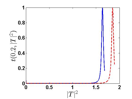
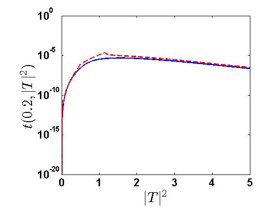
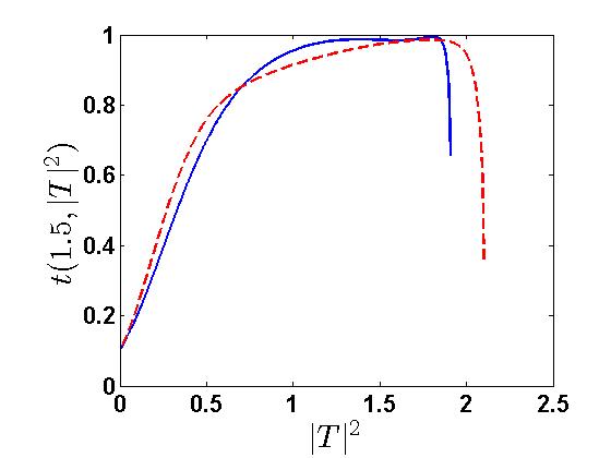
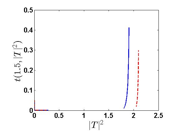
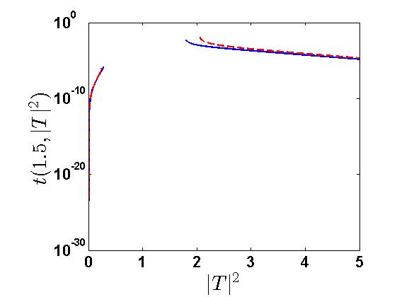
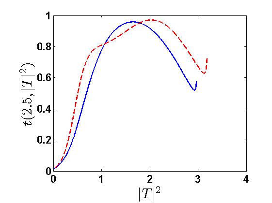
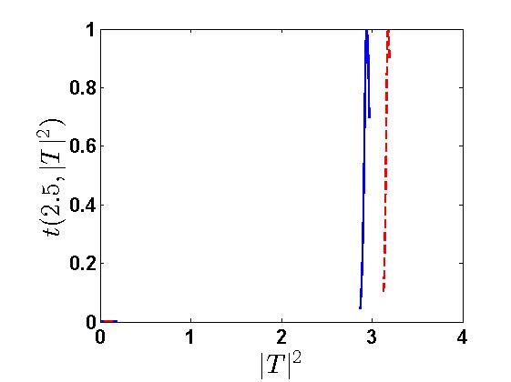
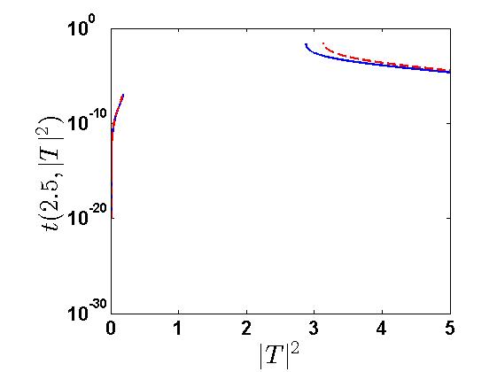
Figure 6: Same as Fig. 5 but for the low saturated case $\beta=0.05$. All other parameters same as before.

For the first transmission channel (middle left Fig. 4 and left vertical panel in Fig. 6), there are only minor differences compared to the ultra-low saturation regime.

For the second channel (middle central Fig. 4 and middle vertical panel in Fig. 6), the major effects appear due to the shrinking of its existence region, for both propagation directions. As a result, for some $k$-values its existence regimes for left and right propagation are fully disjoint, leading to a splitting of the black band in the rectification plot for $\beta=0.01$ into a “triplet band” with white (only right-propagation), orange (no propagation in any direction), and black (only left-propagation) regions appearing in order as $|T|$ is increased. Moreover, the upper cut-off for the low-$|T|$ regime when $k\gtrsim 0.6$ is also slightly larger for the right-propagating wave, leading to the narrow white stripe around $|T|\simeq 0.5$ in middle central Fig. 4. However, transmission is essentially negligible in both directions in the low-$|T|$ regime of the second channel (see middle vertical panel in Fig. 6).

For the third channel (middle right Fig. 4 and right vertical panel in Fig. 6), regimes of non-negligible transmission appear only close to its lower cut-off for larger $k$ (see middle right Fig. 3), which is seen to be somewhat larger for the left-propagating wave. The result is the upper white band in the rectification plot corresponding to only right-propagation, followed for slightly larger $|T|$ by a band with $\mathcal{R}$ close to -1. The lower white stripe is the same as for the second solution since their small-$|T|$ existence regimes are identical.

Medium Saturation, $\beta=0.5$

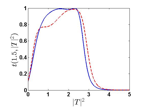
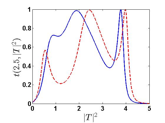
Figure 7: Transmission coefficient $t(k,|T|^{2})$ as a function of $|T|^{2}$ for the medium saturated case $\beta=0.5$, for fixed $k$ values $k=0.2$ (left), $k=1.5$ (middle), $k=2.5$ (right)

.

In this regime, the multi-solution regime is entirely suppressed and thus there is only a single solution for all $k$ and $|T|$. We present the rectifying action in lower Fig. 4 and corresponding plots of transmission coefficient in Fig. 7. The plots are qualitatively similar to those for pure on-site nonlinearity 11 ; wasay18 . Note that the previous black bands in the rectification plots for the first and second solutions in regimes of smaller saturability now have turned into a dark band with $\mathcal{R}$ close to -1, as the narrow transmission peaks in the high-$|T|$ regime now appear for the same solution branch (left Fig. 7). The additional transmission peaks appearing for large $k$ (lower Fig. 3 and right Fig. 7) also lead to a more complicated pattern of regimes with $\mathcal{R}$ alternating between values close to +1 and -1 for increasing $|T|$, when $k$ is close to $\pi$.

VI Stability Analysis

In this section, we investigate the dynamical stability of the stationary solutions used in previous sections. The stability analysis will closely follow as done for instance in lepri ; jd for pure on-site nonlinearities, and it is performed by first perturbing the solutions as

$$A_{n}(t)=P_{n}(t)+\delta R_{n}(t).$$ (27)

This will linearize the equation of motion (1). The resulting linearized set of dynamical equations of order $\delta$ is

$$i\dot{R_{n}}-V_{n}R_{n}+R_{n+1}+R_{n-1}=\gamma_{n}\left(2R_{n}\!\mid\!P_{n}\!\mid^{2}\!+~{}P_{n}^{2}R_{n}^{\ast}\right)+~{}~{}~{}~{}~{}~{}~{}~{}~{}~{}~{}~{}~{}$$

$$\epsilon_{n}\left[\frac{W_{n+1}P_{n}}{(1+\beta|P_{n+1}|^{2}|P_{n}|^{2})^{2}}-\frac{|P_{n+1}|^{4}P_{n}\beta Z}{(1+\beta|P_{n+1}|^{2}|P_{n}|^{2})^{2}}+\frac{R_{n}|P_{n+1}|^{2}}{1+\beta|P_{n+1}|^{2}|P_{n}|^{2}}\right]+~{}~{}~{}~{}~{}~{}$$

$$\epsilon_{n-1}\left[\frac{W_{n-1}P_{n}}{(1+\beta|P_{n-1}|^{2}|P_{n}|^{2})^{2}}-\frac{|P_{n-1}|^{4}P_{n}\beta Z}{(1+\beta|P_{n-1}|^{2}|P_{n}|^{2})^{2}}+\frac{R_{n}|P_{n-1}|^{2}}{1+\beta|P_{n-1}|^{2}|P_{n}|^{2}}\right],$$ (28)

where $W_{n+1}=P^{\ast}_{n+1}R_{n+1}+R^{\ast}_{n+1}P_{n+1}$, $W_{n-1}=P^{\ast}_{n-1}R_{n-1}+R^{\ast}_{n-1}P_{n-1}$ and $Z=P^{\ast}_{n}R_{n}+R^{\ast}_{n}P_{n}$.

With the ansatz $P_{n}(t)=A_{n}e^{-i\omega t},~{}A_{n}\neq A_{n}(t)$ being the complex amplitudes of a stationary solution as before, and $R_{n}(t)=e^{-i\omega t}(a_{n}e^{i\nu t}+b_{n}e^{-i\nu^{\ast}t})$, the linearized set of equations (28) yields an eigenvalue problem of the following form

$$\nu\begin{bmatrix}a_{n}\\ b^{\ast}_{n}\end{bmatrix}=\begin{bmatrix}M_{1}&M_{2}\\ M_{3}&M_{4}\end{bmatrix}.\begin{bmatrix}a_{n}\\ b^{\ast}_{n}\end{bmatrix}.$$ (29)

Specifying to the two nonlinear sites (dimer), the resulting matrices are

$$M_{1}=\begin{bmatrix}\omega-V_{1}-2\gamma_{1}|A_{1}|^{2}+\frac{\epsilon_{1}|A_{2}|^{4}|A_{1}|^{2}\beta}{(1+\beta|A_{1}|^{2}|A_{2}|^{2})^{2}}-\frac{\epsilon_{1}|A_{2}|^{2}}{1+\beta|A_{2}|^{2}|A_{1}|^{2}}&1-\frac{\epsilon_{1}A_{2}^{\ast}A_{1}}{(1+\beta|A_{2}|^{2}|A_{1}|^{2})^{2}}\\ 1-\frac{\epsilon_{1}A_{1}^{\ast}A_{2}}{(1+\beta|A_{1}|^{2}|A_{2}|^{2})^{2}}&\omega-V_{2}-2\gamma_{2}|A_{2}|^{2}+\frac{\epsilon_{1}|A_{1}|^{4}|A_{2}|^{2}\beta}{(1+\beta|A_{1}|^{2}|A_{2}|^{2})^{2}}-\frac{\epsilon_{1}|A_{1}|^{2}}{1+\beta|A_{1}|^{2}|A_{2}|^{2}}\end{bmatrix}$$

$$M_{2}=\begin{bmatrix}-\gamma_{1}A_{1}^{2}+\frac{\epsilon_{1}|A_{2}|^{4}A_{1}^{2}\beta}{(1+\beta|A_{1}|^{2}|A_{2}|^{2})^{2}}&\frac{-\epsilon_{1}A_{2}A_{1}}{(1+\beta|A_{2}|^{2}|A_{1}|^{2})^{2}}\\ \frac{-\epsilon_{1}A_{1}A_{2}}{(1+\beta|A_{1}|^{2}|A_{2}|^{2})^{2}}&-\gamma_{2}A_{2}^{2}+\frac{\epsilon_{1}|A_{1}|^{4}A_{2}^{2}\beta}{(1+\beta|A_{1}|^{2}|A_{2}|^{2})^{2}}\end{bmatrix}$$

$$M_{3}=\begin{bmatrix}\gamma_{1}A_{1}^{\ast 2}-\frac{\epsilon_{1}|A_{2}|^{4}A_{1}^{\ast 2}\beta}{(1+\beta|A_{1}|^{2}|A_{2}|^{2})^{2}}&\frac{\epsilon_{1}A^{\ast}_{2}A^{\ast}_{1}}{(1+\beta|A_{2}|^{2}|A_{1}|^{2})^{2}}\\ \frac{\epsilon_{1}A^{\ast}_{1}A^{\ast}_{2}}{(1+\beta|A_{1}|^{2}|A_{2}|^{2})^{2}}&\gamma_{2}A_{2}^{\ast 2}-\frac{\epsilon_{1}|A_{1}|^{4}A_{2}^{\ast 2}\beta}{(1+\beta|A_{1}|^{2}|A_{2}|^{2})^{2}}\end{bmatrix}$$

and

$$M_{4}\!=\!\begin{bmatrix}-\omega\!+\!V^{\ast}_{1}\!+2\gamma_{1}|A_{1}|^{2}-\frac{\epsilon_{1}|A_{2}|^{4}|A_{1}|^{2}\beta}{(1+\beta|A_{1}|^{2}|A_{2}|^{2})^{2}}+\frac{\epsilon_{1}|A_{2}|^{2}}{1+\beta|A_{2}|^{2}|A_{1}|^{2}}&-1+\frac{\epsilon_{1}A_{2}A^{\ast}_{1}}{(1+\beta|A_{2}|^{2}|A_{1}|^{2})^{2}}\\ -1+\frac{\epsilon_{1}A_{1}A^{\ast}_{2}}{(1+\beta|A_{1}|^{2}|A_{2}|^{2})^{2}}&-\omega\!+\!V^{\ast}_{2}\!+2\gamma_{2}|A_{2}|^{2}-\frac{\epsilon_{1}|A_{1}|^{4}|A_{2}|^{2}\beta}{(1+\beta|A_{1}|^{2}|A_{2}|^{2})^{2}}+\frac{\epsilon_{1}|A_{1}|^{2}}{1+\beta|A_{1}|^{2}|A_{2}|^{2}}\end{bmatrix}.$$

For lattices of size $m$ (with $m=2n+1$ where $n$ is the site counter for each linear side) with this type of nonlinear dimer embedded inside the linear chains to its right and left, the matrices ($M_{1,..,4}$) will be higher dimensional, i.e., $m\times m$. However, apart from the dimer sites the site-dependent coefficients are zero, therefore, in the linear region all entries in $M_{2}$ and $M_{3}$ will be zero, and

$$M_{1} = diag(\omega)+G$$

$$M_{4} = diag(-\omega)-G,$$

where $G$ is an $m\times m$ sparse matrix with ones on both super- and sub-diagonals. The eigenvalue problem corresponding to Eq. (29) is then essentially the eigenvalue computation of the resulting $2m\times 2m$ sparse matrix. This is done by direct numerical computation of the eigenvalues for a finite-sized chain with the nonlinear dimer embedded in the center.

We will present below sample results of this stability analysis for all multi-solution saturation regimes. The eigenvalue/eigenvector computations will be shown for a lattice of 201 sites, and the corresponding time propagation computations have been performed for lattices of up to 2001 sites, in order to accommodate for large $t$-values and avoid boundary errors. As pointed out in lepri , extended eigenvectors corresponding to a continuous spectrum in the infinite-chain limit may cause spurious instabilities due to boundary effects, of the order $1/m$ ($\sim 5\times 10^{-3}$ below). Solutions exhibiting only such unstable eigenmodes thus correspond to linearly stable scattering solutions for the original set-up.

Ultra Low Saturation, $\beta=0.01$

We have chosen $|T|=1$ and $k=0.2,1.5,2.5$ to represent solutions corresponding to small, medium and large wavenumbers respectively, in order to connect with our earlier discussion. The stationary solutions are depicted in Fig. 8, for the three solution branches.

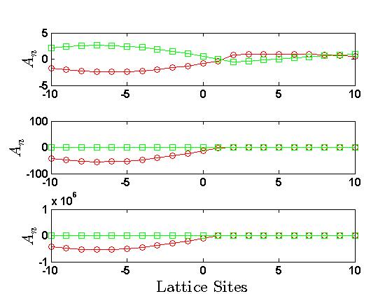
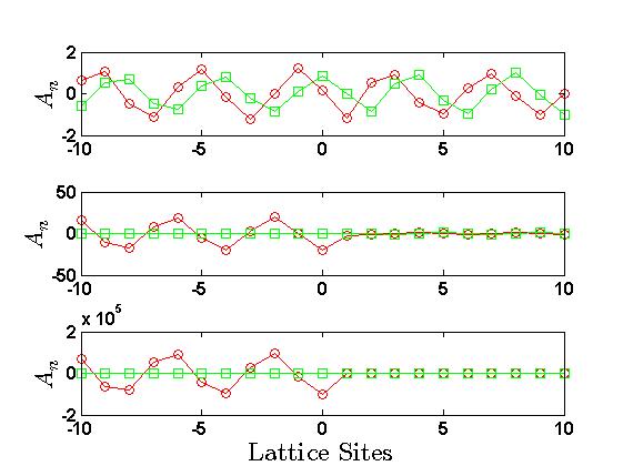
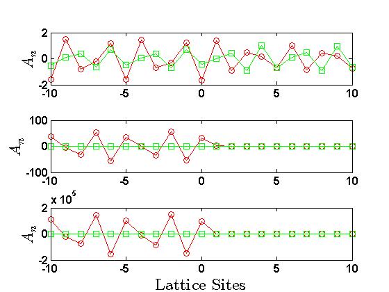
Figure 8: Stationary solutions at $\beta=0.01$, $|T|=1$, real (red circles) and imaginary (green squares) part of the solutions: left vertical panel for $k=0.2$, middle vertical panel for $k=1.5$ and right vertical panel for $k=2.5$. In each vertical panel, top plot corresponds to the first solution branch, middle to the second branch and lower to the third branch.

Note that in this regime, the transmission coefficient is considerable only for the first solution, very small for the second and essentially negligible for the third, for all values of $k$.

Results from the stability analysis are presented in Fig. 9.

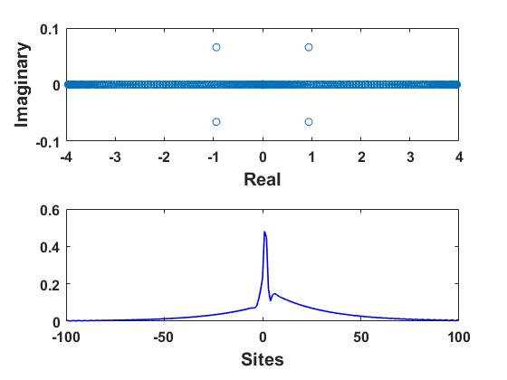
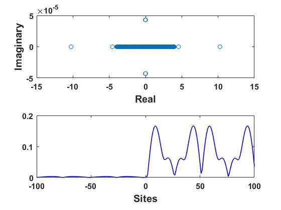
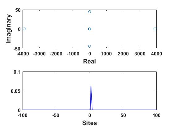
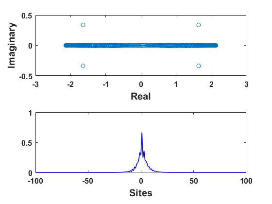
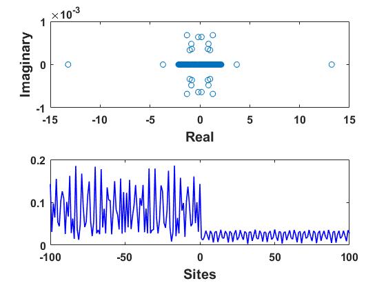
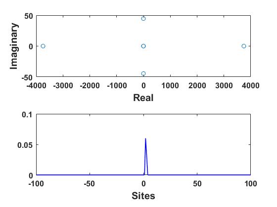
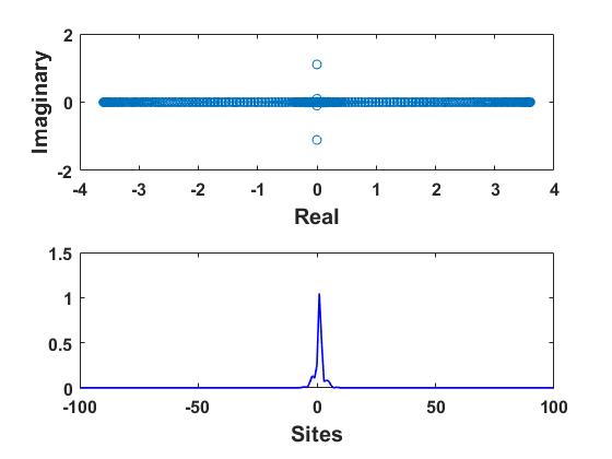
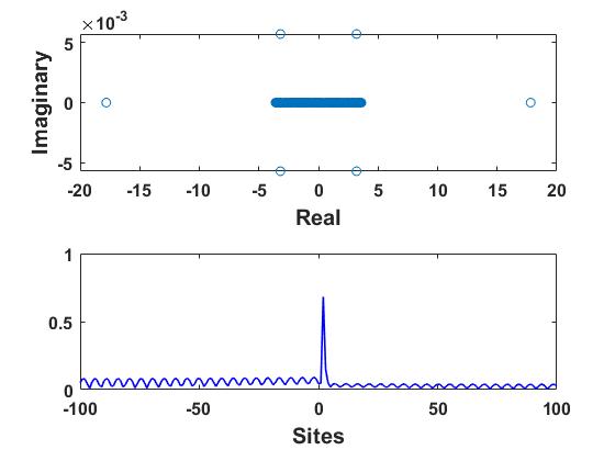
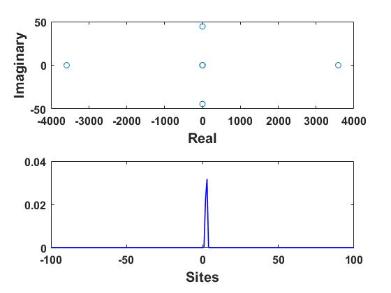
Figure 9: Stability analysis for $|T|=1$ at $\beta=0.01$: $k=0.2$ (first and second row), $k=1.5$ (third and fourth row), $k=2.5$ (fifth and sixth row). Left vertical panel shows the eigenvalues and most unstable eigenvectors for first solution, middle panel for the second solution and right panel for the third solution.

For the first solution (left vertical panel), we find that it is always unstable for these parameter values, with an unstable eigenvector localized at the dimer. For small and intermediate $k$, the unstable eigenvalues are complex corresponding to a rather weak oscillatory instability, while a stronger purely exponential instability appears for larger $k$. The second solution (middle vertical panel) is essentially stable for small and intermediate $k$ (the observed tiny imaginary parts of eigenvalues correspond to extended eigenvectors and are spurious due to boundary effects as discussed above), while a very weak, oscillatory instability appears for larger $k$ due to a resonance between a mode localized at the dimer and the continuous spectrum. The third solution (right vertical panel) is strongly unstable with a purely imaginary eigenvalue, and an eigenmode strongly localized at site 2.

The dynamics resulting from the instabilities of the first solution is illustrated in Fig.10.

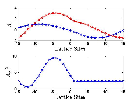
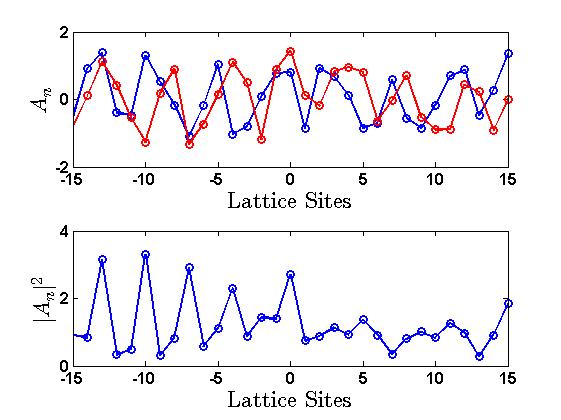
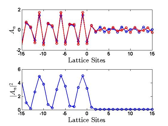
Figure 10: Time propagation corresponding to the first solution in Figs. 8-9; $k=0.2$, $k=1.5$, $k=2.5$ from left to right. Snapshot at time 400 with a small $\mathcal{O}(10^{-3})$ arbitrary perturbation inserted at site 1. Upper figures: Real (blue) and imaginary (red) parts. Lower: $|A_{n}|^{2}$.

For $k=0.2$ we observe that, after an initially oscillatory dynamics with exponentially increasing amplitudes at the center, the solution settles down into an almost stationary transmission regime corresponding to a larger $|T|$ ($|A_{2}|\approx 1.52$ at time 400 in left Fig. 10). However, this value of $|T|$ is above the existence threshold for the first solution at $k=0.2$, and the solution is not strictly stationary but shows small-amplitude oscillations for $|A|$ at the dimer sites, as well as a weak long-wavelength spatial modulation. At $k=1.5$ (middle Fig. 10) the oscillatory instability is stronger and yields persistent spatiotemporal oscillations, while at $k=2.5$ (right Fig. 10) the solution instead, after the initial strong non-oscillatory exponential instability, settles down into an essentially stationary state with considerably smaller $|T|$ ($|A_{2}|\approx 0.27$ at time 400).

The second solution is essentially stable for $|T|=1$, and no significant changes are observed in the time evolution for any of the considered values of $k$.

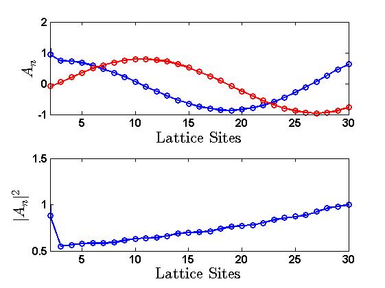
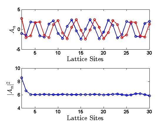
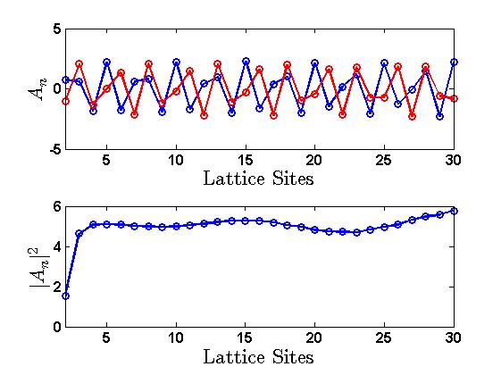
Figure 11: Similar as Fig. 10 but for the third solution in Figs. 8-9, with snapshots at time 40. Only sites 2-30 of a 401-site system are shown.

For the third solution, instability-induced dynamics is illustrated in Fig. 11, where the amplitudes of the initial portion of the transmitting side only (amplitudes at the incoming side are of the order of $10^{5}$ as in Fig. 8) are shown at time 40 (the instability develops rapidly due to the large eigenvalue). Typically, the instability results in an initial decrease of $|A_{2}|$ (where the unstable eigenmode is localized) to values close to zero, followed by recurring oscillations between small and larger amplitudes at this site. As a result of these oscillations the transmitted intensity will start to deviate from 1 as seen previously for the first solution branch; note however from Fig. 11 that now $|A_{n}|<1$ for $k=0.2$ and $|A_{n}|>1$ for $k=1.5$ and $k=2.5$ at the initial portion of the transmitting side (the transmission coefficient evidently remains very small due to the huge amplitudes on the left side).

Low saturation, $\beta=0.05$

We will here pick $|T|=0.4$ as representative for the small-$T$ regime giving three different solutions for each of the sample $k$ values ($k=0.2,1.5,2.5$), and show the stationary solution plots in Fig. 12.

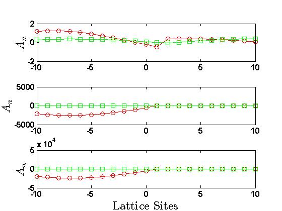
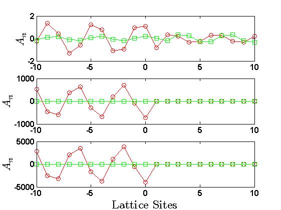
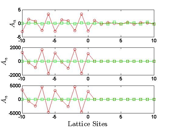
Figure 12: Same as Fig. 8 but with $\beta=0.05$ and $|T|=0.4$.

Note that in this regime, the transmission coefficient is non-negligible only for the first solution.

The stability of each solution in this regime at the respective $k$ values is illustrated in Fig. 13.

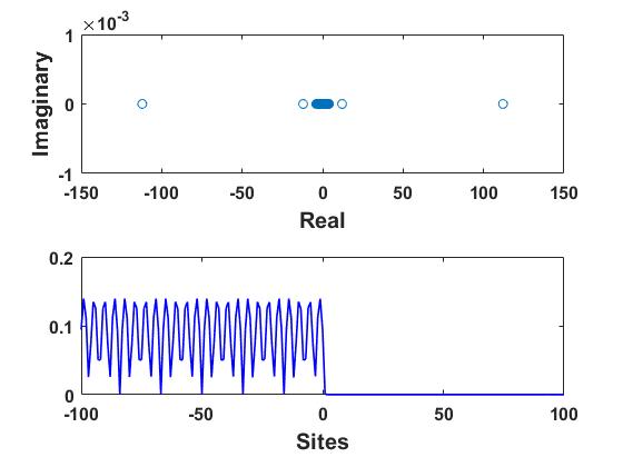
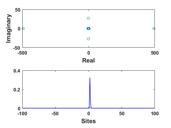
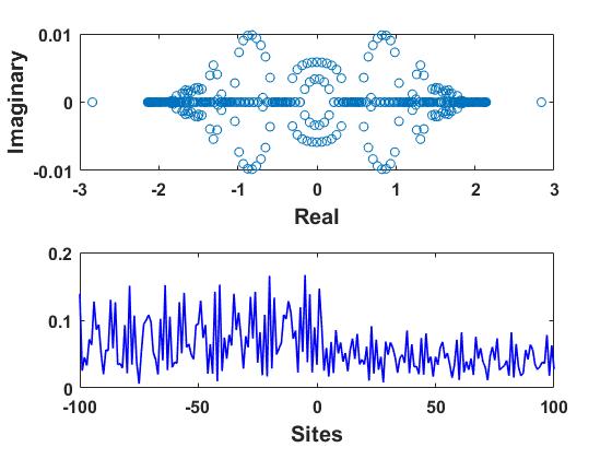
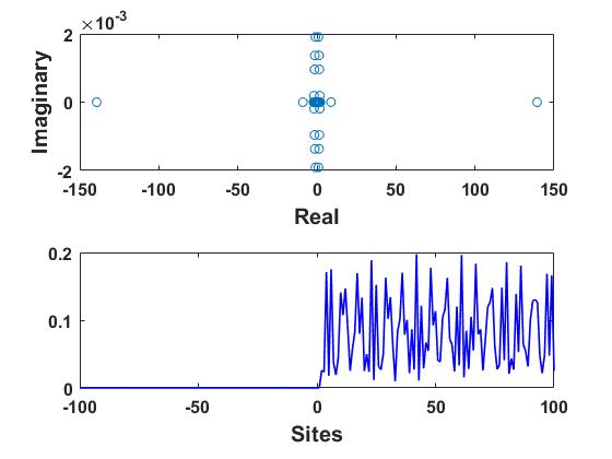
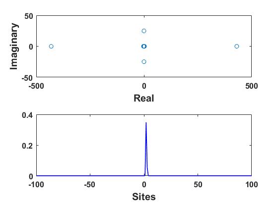
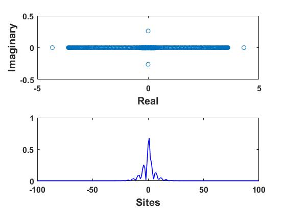
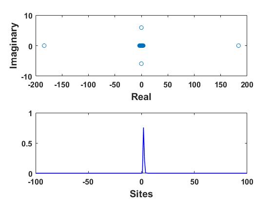
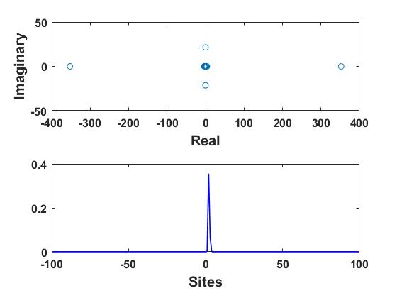
Figure 13: Same as Fig. 9 but with $\beta=0.05$ and $|T|=0.4$.

Comparing to Fig. 9, we note that the instabilities for the first solution here are generally weaker, and to our numerical accuracy it is linearly stable at $k=1.5$ (i.e., for wave numbers close to $\pi/2$). The second solution is still stable for small and intermediate wave numbers, but now destabilizes with a purely imaginary eigenvalue for larger $k$, where it is close to its bifurcation point with the third solution (see Fig. 2). The third solution remains strongly unstable.

To illustrate the outcome of these instabilities, we show in Fig. 14 snapshots of solutions only for unstable cases that differ significantly to those previously shown for $\beta=0.01$ and $|T|=1$. For the first solution at $k=0.2$ (left Fig. 14) the instability is now non-oscillatory, and results in a slight decrease of the amplitude on the transmitting side ($|A_{2}|\approx 0.39$ at time 400). At $k=1.5$ the solution is stable, and at $k=2.5$ the unstable dynamics is analogous to that of Fig. 10. The unstable dynamics of the second solution at $k=2.5$ is illustrated in right Fig. 14 and is similar to that previously described for the third solution, resulting after some transient in amplitudes $|A_{n}|>0.4$ at the initial portion of the transmitting side (the transmission coefficient remaining small with maximal amplitudes $|A_{n}|\sim 2000$ on the left side). For the third solution, dynamics is analogous to that observed in Fig. 11.

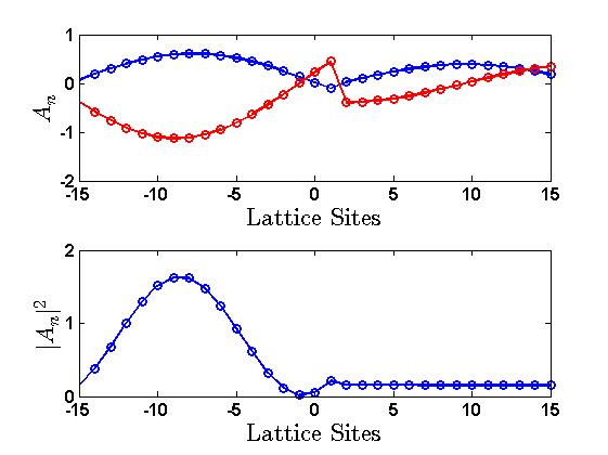
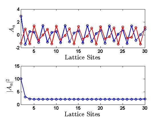
Figure 14: Time propagation of unstable stationary solutions from Figs. 12-13; Left: First solution, $k=0.2$. Right: Second solution, $k=2.5$ (only sites 2-30 are shown). Snapshots at time 400 with a small $\mathcal{O}(10^{-3})$ arbitrary perturbation inserted at site 1. Upper figures: Real (blue) and imaginary (red) parts. Lower: $|A_{n}|^{2}$.

Medium Saturation, $\beta=0.5$

At this saturation strength, only a single-solution regime persists for all $k$ and $|T|$ values. We will pick two representative $|T|$ cases to present the results below, $|T|=1$ and $|T|=2$, to see how the scenario differs for relatively small versus larger intensities. Stationary solution plots are shown in Fig.15.

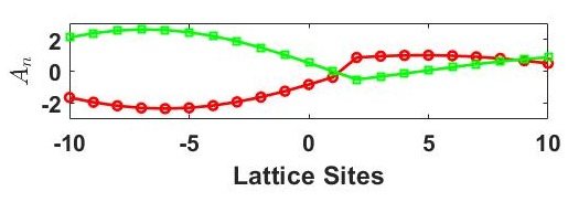
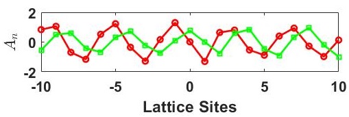
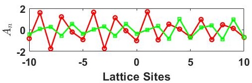
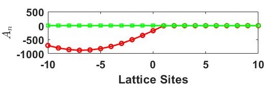
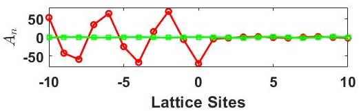
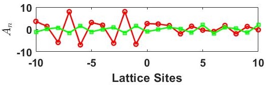
Figure 15: Stationary solutions at $\beta=0.5$, real (red circles) and imaginary (green squares) part of the solutions: Left, middle and right vertical panels for $k=0.2$, $k=1.5$ and $k=2.5$, respectively. Upper horizontal panel corresponds to $|T|=1$, lower to $|T|=2.$.

Note that for $|T|=2$, only the case $k=2.5$ corresponds to a considerable transmission coefficient (cf. Figs. 3, 7)

The stability analysis with corresponding examples of unstable time propagation for the case of $|T|=1$ and the three sample $k$ values is presented in Fig.16.

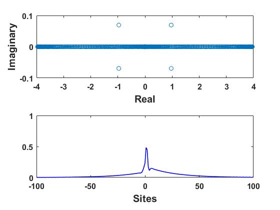
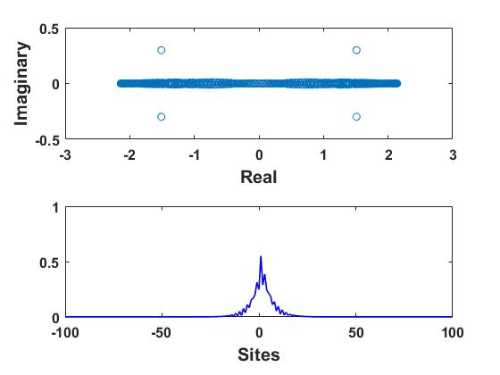
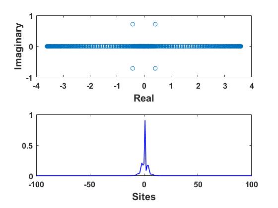
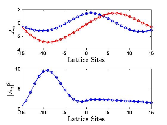
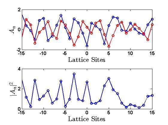
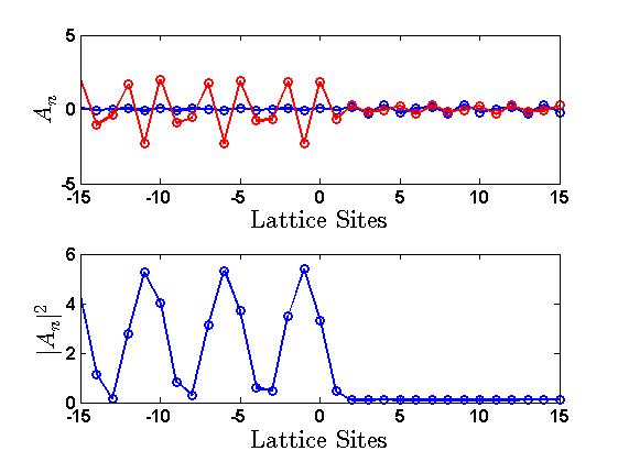
Figure 16: Top two horizontal panels: Stability analysis for $|T|=1$ and $\beta=0.5$, with eigenvalues at top and most unstable eigenvectors at second row. Left, middle and right plots correspond to $k=0.2$, $k=1.5$ and $k=2.5$, respectively. Lower two horizontal panels: snap shots of time propagation for the corresponing values of $k$ (at time 200 for $k=0.2$ and 100 for $k=1.5,2.5$). Third row: real (blue) and imaginary (red) parts; fourth row: $|A_{n}|^{2}$.

Comparing with Figs. 9-10, we note that the scenario is very similar to that of the first solution for the same value of $|T|$ when $\beta=0.01$; the main qualitative difference is seen for $k=2.5$ where the instability now is oscillatory and slightly weaker. Thus, we may conclude that as long as the amplitudes at the dimer sites are moderate, which will typically be the case when $|T|$ is relatively small and transmission coefficient $t$ is relatively large, the scenario in the regime of medium saturation is qualitatively similar to that for the first solution branch for weaker saturability.

The case of various sample $k$ at higher intensities ($|T|=2$) is shown in Fig. 17.

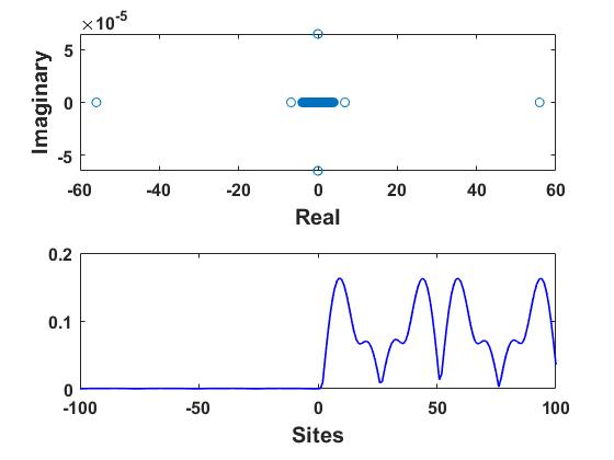
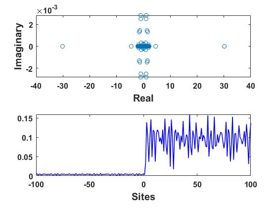
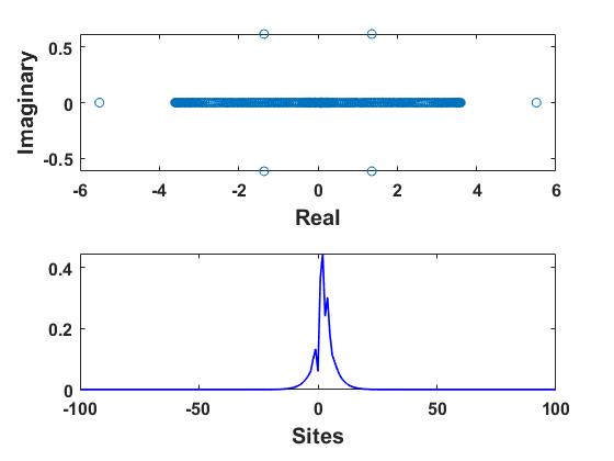
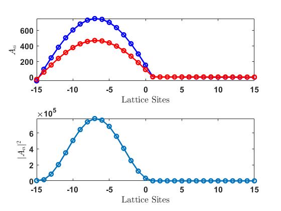
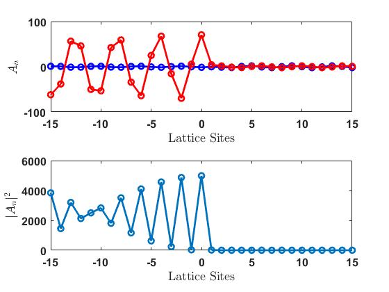
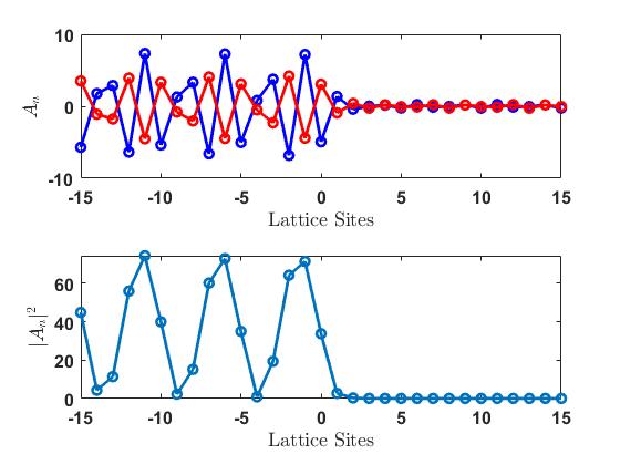
Figure 17: Similar as Fig. 16 but for $|T|=2$. The snapshots for time propagation plots are all at time 300.

For $k=0.2$ (left Fig. 17) and $k=1.5$ (middle Fig. 17) the solution is now stable (but with very small transmission coefficient), while for $k=2.5$ (right Fig. 17) the instability scenario is similar as above for $|T|=1$, resulting after some time in an almost stationary transmission with considerably smaller amplitudes at the transmitted side of the dimer ($|A_{2}|\approx 0.57$ at time 300).

Summarizing this section, we note some similarities and differences compared to previously reported stability results for pure on-site nonlinearities lepri ; jd . As in lepri ; jd , we observe that the exactly stationary propagating solutions are unstable in regimes where the transmission coefficient is significant. Stationary waves having small transmission coefficient appear typically as stable as noted in lepri ; jd , except in the multisolution regimes where the third solution branch (which has no counterpart neither for systems with pure on-site nonlinearity, nor with unsaturated inter-site nonlinearities) is generally unstable, and the second solution branch destabilizes close to its bifurcation with the third solution. As long as the instability is weak, it is typically oscillatory (complex eigenvalues) as originally reported in lepri . In regimes of stronger instabilities eigenvalues become purely imaginary, as also seen for the saturable on-site nonlinarity in jd . However, a major difference is that in all cases reported in lepri ; jd for on-site nonlinearities, the instability resulted in a trapped, localized defect mode at the central nonlinear sites. As seen above, none of the here considered instability regimes resulted in any significant trapping at the dimer. Thus, it appears that inter-site nonlinearities generally counteract the creation of a localized dimer mode. Another difference is that in jd , it was concluded that instabilities generically (for on-site saturable oligomers) appeared to transport power to the right part of the lattice for $k>0$ (thus decreasing the power of the part immediately to the left of the dimer). Here, we observe this scenario in some cases (mainly for first solution branch with small $k$ when instability is oscillatory, and third branch at larger $k$), while in other cases the scenario is opposite with a decrease of power at the right side (e.g., for large $k$ in the single-solution regime and for first solution in multi-solution regime, and for small $k$ for third solution). Thus, even though the transmission coefficient for stationary transmission in the regime of medium saturation (Figs. 3, 7) looks qualitatively similar to the on-site nonlinearity cases, the instability-induced dynamics may be quite different.

VII Propagation of an initial Gaussian

As an example different from the stationary plane wave solutions we investigate, by direct numerical integration of Eq. (1), the time propagation of an initial Gaussian wavepacket through the chain with the dimer defect having saturated inter-site nonlinear interactions between the two dimer sites. The initial Gaussian data is

$$A_{n}(0)=I~{}\textmd{exp}\left[-\frac{\left(n-n_{0}\right)^{2}}{w^{2}}+ik_{i}n\right],$$ (30)

where $I$ and $p$ are the amplitude and width of the initial wave-packet taken to be $\sqrt{3}$ and $56$, respectively. Typical results for this initial condition with $|k_{0}|=\pi/2$ (corresponding to maximum propagation speed and minimum dispersion) in the regimes of low ($\beta=0.05$) and medium ($\beta=0.5$) saturation are shown in Fig. 18. (Results in the ultra-low saturation regime are very similar to those for $\beta=0.05$.)

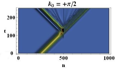
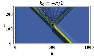
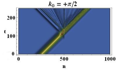
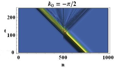
Figure 18: Color plots of $|A_{n}(t)|^{2}$ as a function of $n$ (lattice sites) and $t$ (time), with the Gaussian initial data of Eq. (30), saturation $\beta=0.05$ (upper horizontal panel) and $\beta=0.5$ (lower horizontal panel); wavenumber $k_{0}=\pm\frac{\pi}{2}$, and all other parameters as before. Left (right) vertical panel corresponds to the cases with left (right) incidence. The dimer is located at sites 501 and 502 in a 1000 site lattice.

The transmission coefficient for the wavepacket is defined as in 11 to be the ratio of transmitted power to the initial input power. For the case of right propagating signal, it is given by

$$\tau_{+}=\frac{\sum_{i>\frac{n}{2}+2}|A_{i}(t_{f})|^{2}}{\sum_{i<\frac{n}{2}+1}|A_{i}(0)|^{2}},$$ (31)

where $n$ is the total number of sites, the dimer is located at sites $n/2+1$ and $n/2+2$, and $t_{f}$ the final time for the numerical integration. Equation (31) can be understood by a direct analogy with Eq. (19). For $\beta=0.05$, the transmission coefficient for the left incidence (right propagating case; top left plot in Fig. 18) is found to be $\tau_{+}=0.474$. In an analogous way, the transmission coefficient for the right incidence (left propagating) case depicted in the top right plot in Fig. 18 turns out to be $\tau_{-}=0.603$. The rectifying factor is computed by the formula $f=\frac{\tau_{+}-\tau_{-}}{\tau_{+}+\tau_{-}}$, in analogy with Eq. (26), which in this case is found to be $f=-0.120$. The distinct left and right transmission coefficients reflect the fact that the parity symmetry of the dimer defect is indeed broken. The lower horizontal panel in Fig. 18 corresponds to the regime of medium $\beta$ strength ($\beta=0.5$). The transmission coefficients are found to be $\tau_{+}=0.797$ and $\tau_{-}=0.819$, and the corresponding rectifying factor is found to be $f=-0.013$. Thus, increasing saturation implies that the transmission increases but the asymmetry decreases significantly, as was also found in previous works for on-site saturability Erik ; wasay3 . This is also consistent with results for the stationary transmission, e.g., by comparing middle left plot in Fig. 6 and middle plot in Fig. 7. For $\beta=0.05$ and $|k|$ close to $\pi/2$ (Fig. 6) there is essentially no transmission with $|T|^{2}>2$, and thus the peak intensity of the Gaussian with $I^{2}=3$ cannot be transmitted, while for $\beta=0.5$ (Fig. 7) there is almost complete transmission around $|T|^{2}=2.5$, allowing for a larger portion of the Gaussian to be transmitted. On the other hand, the main transmission around $|T|^{2}=2.5$ for $\beta=0.5$ is almost symmetric for left- and right-propagation, while for $\beta=0.05$ the stationary transmission for right-propagation (blue curve) dips sharply around $|T|^{2}=1.8$, while for left-propagation (red curve) the dip appears later, around $|T|^{2}=2$. Thus, a considerable part of the Gaussian with $I^{2}=3$ may be transmitted to the left but not to the right. (Weak instabilites of the stationary transmission modes described in previous section will not significantly affect the transmission of a rapidly moving and not too wide Gaussian, if the time for the Gaussian to pass the dimer will be shorter than the time for the instability to develop.)

It should also be noted from Fig. 18 that, in addition to partial transmission/reflection of the Gaussian and creation of small-amplitude radiation waves, a rather small part will remain trapped at the dimer sites. For the cases shown in Fig. 18, we find at time $t_{f}=250$ the trapped intensity $P_{trap}\equiv|A_{501}|^{2}+|A_{502}|^{2}$ to be: $P_{trap}(\beta=0.05,k=+\pi/2)=0.77$, $P_{trap}(\beta=0.05,k=-\pi/2)=2.17$, $P_{trap}(\beta=0.5,k=+\pi/2)=2.79$ $P_{trap}(\beta=0.5,k=-\pi/2)=2.29$. Thus, in these cases considerably less trapping appears in the case when the main part is reflected, compared to when it is mainly transmitted. This is opposite to the example considered in 11 , where trapping was enhanced when the main part was reflected. We may also note that for on-site saturabilites, increasing saturation strength typically decreases trapping Erik , while we here observed an opposite tendency (which might be intuitively understood as increasing the saturability of the inter-site nonlinearity implies that the on-site nonlinearity will be relatively more important, and trapping is in general mainly associated with on-site nonlinearities).

Note also that the transmission coefficient typically is largest when the incoming Gaussian first encounters the dimer site with smallest $|V_{2}|$, i.e., the site where the deviation from the linear chain with zero on-site potential is smallest. Intuitively this seems reasonable, and an analogous remark was made for a saturable on-site potential in jd . We checked a few other parameter values and obtained analogous results. Keeping $V_{1}=-2.625$ and changing the on-site amplitude on the right dimer site to $V_{2}=-1.875$ (i.e., decreasing its magnitude), we obtained for $\beta=0.05$ that $\tau_{+}=0.594$ and $\tau_{-}=0.746$ with rectifying factor $f=-0.113$, i.e., transmission increases while rectification remains almost the same (and with the same sign). On the other hand, changing the on-site amplitude at the right dimer site to $V_{2}=-3.125$ (i.e., increasing its magnitude to have $|V_{2}|>|V_{1}|$) resulted in $\tau_{+}=0.722$ and $\tau_{-}=0.542$ with $f=+0.143$. This means that the diode-like transmission in the low-saturation regime, as expected, gets reversed when $|V_{2}|>|V_{1}|$.

VIII Conclusions

The main aim of this work has been to provide a clear and comprehensive description of qualitatively novel effects that appear in the transmission scenario of a DNLS-type dimer when nonlinear coupling between the dimer sites is taken into account, in addition to a standard onsite (cubic) nonlinearity. For the generality of the description, we considered a saturable intersite nonlinearity, with a parameter $\beta$ interpolating between a purely cubic intersite + onsite nonlinearity at $\beta=0$, and a cubic pure onsite nonlinearity at large $\beta$. A major novel result is that, in contrast to the commonly studied cases with pure onsite nonlinearity, the transmission coefficient for stationary transmission is in general no longer a single-valued function of the transmitted intensity $|T|$, as the standard backward transfer map in regimes of small and moderate $|T|$ and low saturation will have three distinct solutions (two in the case of strictly zero saturation). These solutions differ in their relative phase shift across the dimer. As the saturation increases, solutions disappear through bifurcations at critical saturation strengths (depending on the wave number), leaving a single solution branch in regimes of medium and strong saturation.

We analyzed numerically the transmission coefficient of the three different branches, and showed how these merged into the single-valued (as a function of $|T|$) transmission picture, known from previous works, as saturation strength increased. We also performed a linear stability analysis of the stationary scattering solutions. In low-saturation regimes with three solution branches, one branch, with very small transmission, exhibited strong instabilities, while from the other two branches solutions with small transmission coefficients were typically stable, and those with larger transmission exhibited rather weak instabilites, growing larger when approaching transmission peaks. Qualitatively the results for the latter two branches agree with previous work for pure onsite DNLS. Studying by direct numerical simulations the effect of the instabilities on the transmission, two notable differences to previous works were found as a result of the intersite nonlinearities: (i) we did not observe any significant trapping at the dimer sites; (ii) while previous works always found transport of power towards the transmission side, in some regimes we instead found transport of power towards incoming/reflected side.

We also analyzed the left/right asymmetries in the transmission coefficient with different linear onsite potentials at the dimer sites, both for stationary plane waves and for rather wide and rapidly moving Gaussian excitations with amplitiude near the main transmission threshold. In addition to shifting the location of transmission peaks, the multiple transmission branches for low saturability leads to a novel rectification effect for stationary transmission, where a transmission peak in one direction, for a given branch and a given $|T|$, may correspond to non-existence of solutions in the opposite propagation direction for this branch. For the Gaussian propagation, we found that increasing saturation strength typically would increase the transmission coefficient but decrease the rectifying factor, as the stationary transmission spectrum also became broader and more symmetric for wave vectors close to $\pi/2$.

Finally, we also comment on possible applications of our work. Our choice of model arose from the interest in studying the gradual transition from a system with non-saturated to saturated intersite nonlinearities, keeping onsite nonlinearities non-saturated. The saturability is typically in the form appearing from photovoltaic-photorefractive materials, which may be a suitable class of systems where the phenomenology of multichannel asymmetric transmission described here may be observed. A relevant topic for future research would be to perform a similar analysis for the type of saturable nonlinear couplings proposed in Hadad17 , with direct application to electric circuit ladders Hadad18 .

*

Appendix A Slightly increasing/decreasing $V_{2}$ at $\beta=0.01$

To exemplify how the stationary transmission scenario for left- and right-propagating waves changes when the linear onsite potential on the dimer sites is varied, we consider the transmission curves at $\beta=0.01$ and first increase $V_{2}$ by setting $V_{2}=V^{(0)}(1-5\varepsilon)$($=-1.8750$), where $\varepsilon$ is the asymmetry held at $\varepsilon=0.05$, and $V^{(0)}=-2.5$. Note that $V_{1}$ remains at $V_{2}=V^{(0)}(1+\varepsilon)(=-2.6250)$, as in the whole paper. The transmission curves corresponding to all three solution branches for all three representative $k$ are shown in Fig. 19. Compared with the ones in Fig. 5, where $V_{2}$ was kept at $V_{2}=V^{(0)}(1-\varepsilon)(=-2.3750)$, we first note that increasing $V_{2}$ shrinks the multi-solution regime for the right-propagating waves (blue curves) but does not change the existence regimes for left-propagating waves (red curves). This is simply a consequence of the fact that (20) contains $V_{2}$ but not $V_{1}$.

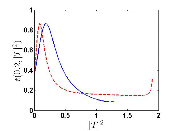
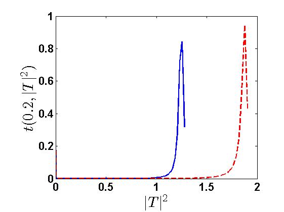
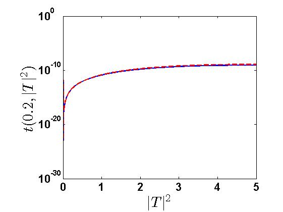
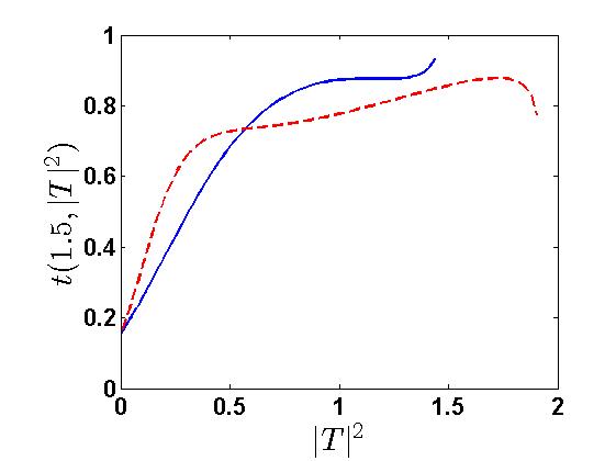
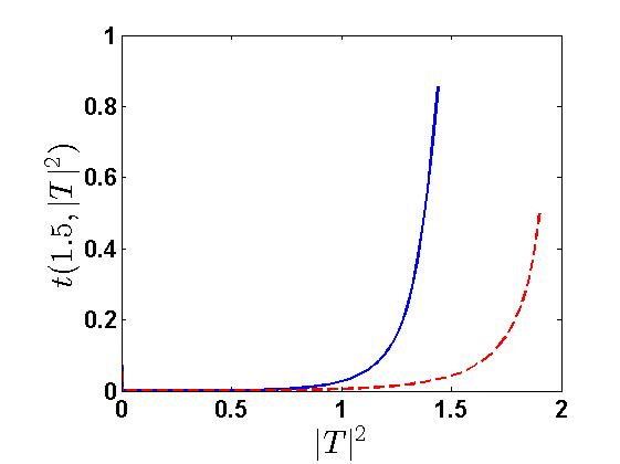
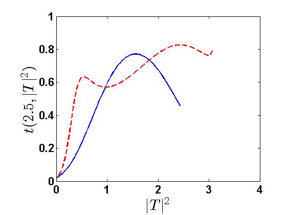
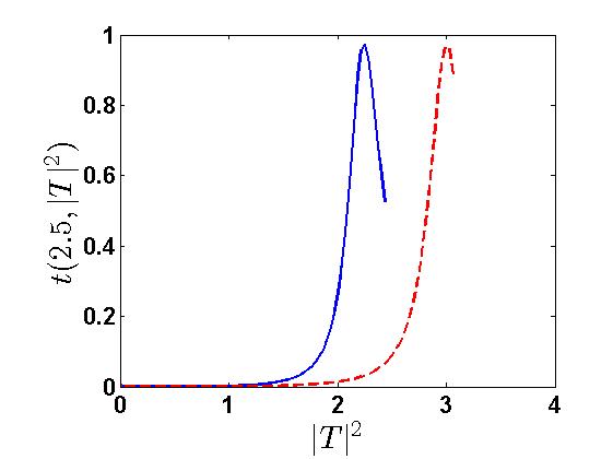
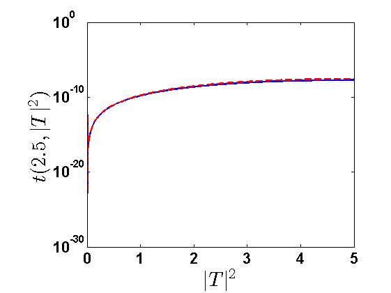
Figure 19: Same as Fig.5, except $V_{2}$ has been increased to -1.8750.

The transmission coefficent however depends on both $V_{1}$ and $V_{2}$ for both directions of propagation, and is overall decreased as $|V_{1}-V_{2}|$ increases. Thus, rectification effects increase, but to the price of narrower transmission peaks and lower total transmission.

The case of decreasing $V_{2}$ to $V_{2}=V^{(0)}(1+5\varepsilon)(=-3.1250)$ is shown in Fig. 20.

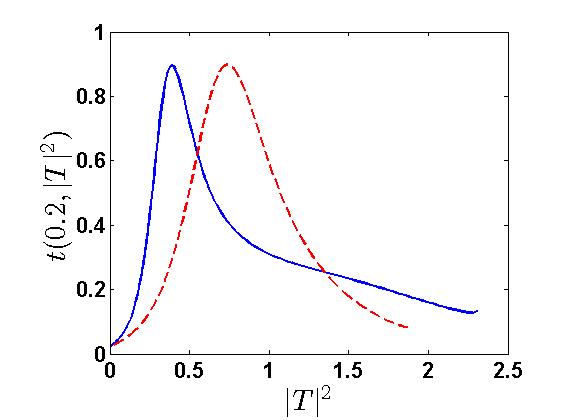
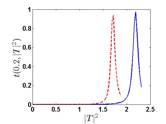
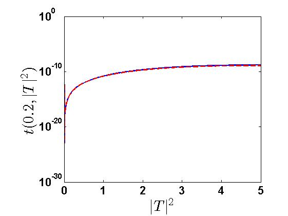
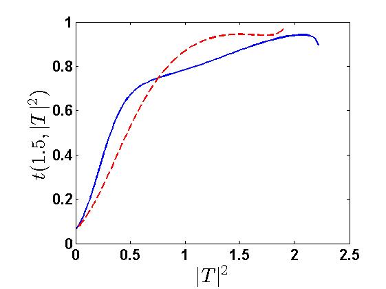
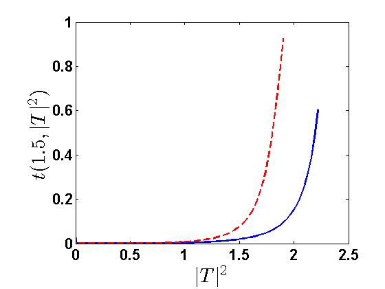
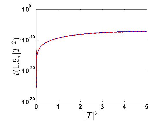
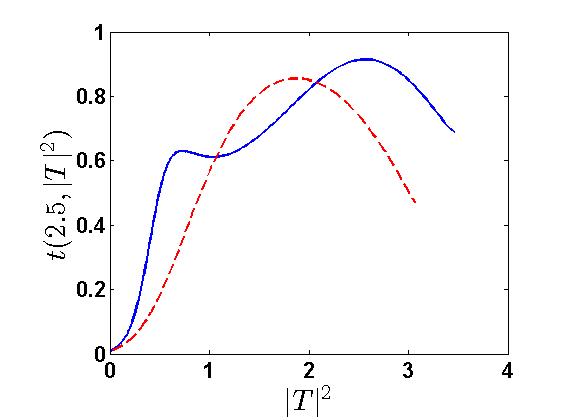
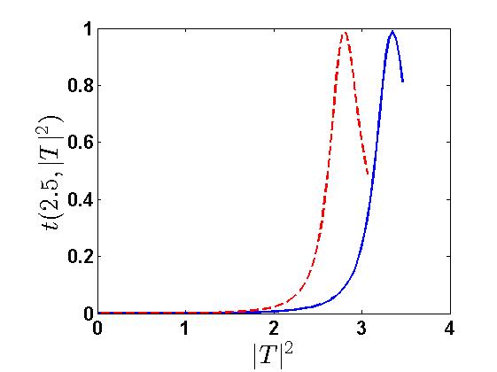
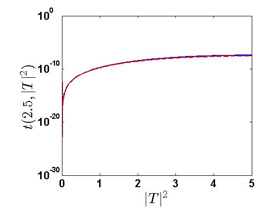
Figure 20: Same as Fig. 5, except $V_{2}$ has been decreased to -3.1250.

We note that decreasing $V_{2}$ results in the persistence of multi-solutions for a longer stretch of intensities for right-propagating waves. In addition to this, since now $|V_{2}|>|V_{1}|$ the main transmission scenario gets reversed between the left and right incidence, as compared to Fig. 5. Generally, the transmission regime appears wider when the incoming wave first hits the site with smallest magnitude of the linear on-site potential.

References

- [1] S. Trillo and S. Wabnitz, Appl. Phys. Lett. 49, 752 (1986); 51, 60 (1987).
- [2] S. Lepri and G. Casati, Phys. Rev Lett. 106, 164101 (2011).
- [3] S. Lepri and G. Casati, in R. Carretero-González et al. (Eds.): Localized Excitations in Nonlinear Complex Systems: Current State of the Art and Future Perspectives (Springer, Cham, Switzerland, 2014), p. 63; arXiv:1211.4996.
- [4] F. Delyon, Y.-E. Lévy, and B. Souillard, Phys. Rev Lett. 57, 2010 (1986).
- [5] Y. Wan and C. M. Soukoulis, Phys. Rev. B 40, 12264 (1989); Phys. Rev. A 41, 800 (1990).
- [6] G. Tsironis and D. Hennig, Phys. Rep. 307, 333 (1999).
- [7] T. F. Assunção, E. M. Nascimento, and M. L. Lyra, Phys. Rev. E 90, 022901 (2014).
-
[8]
E. Johansson, Diploma thesis, Linköping University,
http://urn.kb.se/resolve?urn=urn:nbn:se:liu:diva-111236 (2014). - [9] D. Law, J. D’Ambroise, P.G. Kevrekidis, and D. Kip, Photonics 1, 390 (2014).
- [10] M. A. Wasay, Sci.Rep. 8, 5987 (2018).
- [11] M. A. Wasay, M. L. Lyra, and B. S. Ham, Sci.Rep. 9, 1871 (2019).
- [12] N. Li and J. Ren, Sci. Rep. 4, 6228 (2014).
- [13] G. Wu, Y. Long and J. Ren, Phys. Rev. B 97, 205423 (2018).
- [14] H. Yan, G. Wu and J. Ren, Phys. Rev. E 100, 012207 (2019).
- [15] M. Öster, M. Johansson, and A. Eriksson, Phys. Rev. E 67, 056606 (2003).
- [16] A. Smerzi and A. Trombettoni, Phys. Rev. A 68, 023613 (2003).
- [17] G. Gligorić, A. Maluckov, Lj. Hadžievski, and B. A. Malomed, Phys. Rev. A 78, 063615 (2008).
- [18] S. Rojas-Rojas, R. A. Vicencio, M. I. Molina, and F. Kh. Abdullaev, Phys. Rev. A 84, 033621 (2011).
- [19] M. Johansson, Physica D 216, 62 (2006).
- [20] F. Kh. Abdullaev, Yu. V. Bludov, S. V. Dmitriev, P. G. Kevrekidis, and V. V. Konotop, Phys. Rev. E 77, 016604 (2008).
- [21] M. A. Wasay, Phys. Rev. E 96, 052218 (2017).
- [22] G. C. Valley, M. Segev, B. Crosignani, A. Yariv, M. M. Fejer, and M. C. Bashaw, Phys. Rev. A 50, R4457 (1994).
- [23] Y. Hadad, V. Vitelli, and A. Alu, ACS Photonics 4, 1974 (2017).
- [24] Y. Hadad, J. C. Soric, A. B. Khanikaev, and A. Alù, Nature Electronics 1, 178 (2018).
- [25] J. C. Eilbeck and M. Johansson, in Localization and Energy Transfer in Nonlinear Systems, Proceedings of the Third Conference, San Lorenzo de El Escorial Madrid, edited by L. Vázquez, R. S. MacKay, and M. P. Zorzano (World Scientific, Singapore, 2003), p. 44.
*