Multilevel Monte Carlo with Numerical Smoothing for Robust and Efficient Computation of Probabilities and Densities

Abstract

The multilevel Monte Carlo (MLMC) method is highly efficient for estimating expectations of a functional of a solution to a stochastic differential equation (SDE). However, MLMC estimators may be unstable and have a poor (noncanonical) complexity in the case of low regularity of the functional. To overcome this issue, we extend our previously introduced idea of numerical smoothing in (Quantitative Finance, 23(2), 209-227, 2023), in the context of deterministic quadrature methods to the MLMC setting. The numerical smoothing technique is based on root-finding methods combined with one-dimensional numerical integration with respect to a single well-chosen variable. This study is motivated by the computation of probabilities of events, pricing options with a discontinuous payoff, and density estimation problems for dynamics where the discretization of the underlying stochastic processes is necessary. The analysis and numerical experiments reveal that the numerical smoothing significantly improves the strong convergence, and consequently, the complexity and robustness (by making the kurtosis at deep levels bounded) of the MLMC method. In particular, we show that numerical smoothing enables recovering the MLMC complexities obtained for Lipschitz functionals due to the optimal variance decay rate when using the Euler–Maruyama scheme. For the Milstein scheme, numerical smoothing recovers the canonical MLMC complexity even for the nonsmooth integrand mentioned above. Finally, our approach efficiently estimates univariate and multivariate density functions.

Keywords Multilevel Monte Carlo, numerical smoothing, probability estimation, density estimation, robustness, complexity, Monte Carlo, option pricing

2010 Mathematics Subject Classification 62P05, 65C05, 65D30, 65Y20, 91G20, 91G60.

1 Introduction

In several applications such as probability computation, distribution functions or density estimation, digital/barrier option pricing, sensitivity computation (particularly financial Greeks), and risk estimation, one is interested in efficiently computing the expectation of a functional $g$ of a solution, $X$, to a stochastic differential equation (SDE):

(1.1) $$\mathrm{E}\left[g(X)\right],$$

even when $g$ exhibits low regularity.

Monte Carlo (MC) methods (standard and multilevel MC (MLMC) [21]) can be used to approximate the expectation in (1.1). Although the convergence rate of the standard MC method is insensitive to the input space dimensionality and regularity of the functional $g$, the convergence is slow. In contrast, the MLMC method (based on a hierarchical representation of the expectation of interest and with a better convergence speed than the standard MC method) is negatively affected by the low regularity of $g$. These adverse effects consist of (i) a nonoptimal variance decay rate that affects the complexity of the MLMC method (see [4, 24, 22] and Sections 3 and 4) and (ii) a high kurtosis at the deep levels of MLMC, which deteriorates the robustness and performance of the estimator (see Sections 3 and 4). Furthermore, when estimating densities ($g$ in (1.1) is a Dirac delta function), standard (without smoothing) or regularized MC and MLMC methods either fail due to infinite variance or have an error that explodes with the dimensions (see Section 2.3).

This work addresses the mentioned challenges for cases where analytic (bias-free) smoothing of the integrand cannot be performed. We extend our numerical smoothing idea introduced in [7] to the MLMC estimator to improve its robustness and complexity when computing the expected value of a discontinuous function, particularly when computing probabilities, estimating densities or pricing options with discontinuous payoffs. This technique, previously introduced in [7] in the context of deterministic quadrature methods, is based on root-finding methods combined with a one-dimensional (1D) numerical integration with respect to (w.r.t.) a single well-chosen variable.

Previously, the authors of [4, 24] used the MLMC method without smoothing for pricing options with discontinuous payoffs and obtained poor performance (worst-case complexity of the MLMC method). Afterward, various treatments [16, 38, 25, 2, 35, 30] were proposed to deal with discontinuous functionals efficiently when using the MLMC method. These methods can be classified as follows: (i) methods based on adaptivity and branching ideas [30, 23], which require specialized design for specific problems, (ii) methods based on conditional smoothing with respect to the last Brownian motion increments as in [19, 38], where the smoothing effect vanishes as the time step size $\Delta t\rightarrow 0$, and (iii) methods based on parametric regularization and kernel smoothing ideas as in [25], which may suffer from exponential error growth with respect to the dimension of the underlying process (as explained in Section 2.3). For instance, [38] used implicit smoothing based on conditional expectation tools. Although this technique improved the variance decay rate and complexity of MLMC when using the Milstein scheme, it did not help with the Euler discretization. Furthermore, in general cases, the dynamics may make it difficult to derive an analytic expression for the conditional expectation of interest. Using the Milstein scheme may have major drawbacks: (i) it is expensive to compute for high-dimensional dynamics due to the Lévy areas terms; (ii) the design of a suitable coupling strategy is challenging; and (iii) the kurtosis may explode at the deep levels. The authors of [25] suggested a different approach based on parametric smoothing. They carefully constructed a regularized version of the functional, based on a regularization parameter that depends on the degree of smoothness of the function of interest. Despite offering better performance than the standard (without smoothing) MLMC estimator and a clear setting for the theoretical analysis, this approach has a practical disadvantage regarding the difficulty of its generalization toward the cases where (i) no prior knowledge of the degree of smoothness of the function of interest exists and (ii) more challenging dynamics are considered than the geometric Brownian motion (GBM). We refer to [22] for a detailed review of the various MLMC ideas employed when computing an expected value of a discontinuous function.

We mention that other similar and different smoothing techniques were previously proposed for deterministic quadrature techniques (e.g., bias-free, conditional sampling, and preintegration) to improve the performance of deterministic quadrature techniques (e.g., (adaptive) sparse grid quadrature and quasi-Monte Carlo (QMC)) for the applications of option pricing with discontinuous payoffs [1, 40, 29, 8, 5, 7, 6] and estimating univariate density of random variables (rdvs) [9, 18, 37]. However, the focus of this work is to propose a different approach than in [16, 38, 25, 2, 35, 30] to improve the performance of MLMC methods when computing an expected value of a discontinuous function with applications in probability computation, digital option pricing and univariate/multivariate density estimation.

The main contributions of this work are summarized as follows:

• Compared with the case without smoothing, this analysis reveals that the employed numerical smoothing technique improves (i) the convergence of the variance of MLMC, (ii) the complexity of the MLMC estimator owing to the improvement in the variance decay rate and (ii) the robustness of the estimator by significantly reducing and better controlling the kurtosis at deep levels (making it bounded). In particular, we theoretically (see Theorems 3.7 and 3.8) and numerically demonstrate that numerical smoothing enables recovering the MLMC complexities obtained for Lipschitz functionals by proving that the optimal variance decay rate is recovered when using the Euler–Maruyama scheme. Using the Euler scheme, we obtain rates of variance decay and MLMC complexity similar to those reported in [19, 38] without employing higher-order schemes, such as the Milstein scheme. For the Milstein scheme, we numerically illustrate that numerical smoothing recovers the canonical MLMC complexity.

• The proposed approach efficiently estimates univariate and multivariate density functions: a task that previous MC-or MLMC-based methods either fail to achieve due to the infinite variance or have an error that explodes with the dimension when using parametric smoothing or kernel density ideas. Estimating densities using the MLMC method in [25] results in a mean squared error (MSE) behavior similar to that obtained using kernel density techniques, where the error increases exponentially w.r.t. the dimension of the underlying process. However, due to the exact conditional expectation w.r.t. the Brownian bridge, the error of our approach is restricted to the root-finding error when approximating the discontinuity location, which does not increase exponentially w.r.t. the dimension (see Section 2.3 for further details). Although we provide pointwise density estimates, the proposed approach can be easily extended to approximate functions using similar ideas as in [25, 35] using interpolation grids.

• Unlike [9, 18, 37], which only considered the problem of estimating univariate density of rdvs using the QMC method, the proposed approach is based on the MLMC idea and is designed for estimating univariate/multivariate densities for dynamics where the discretization of the underlying stochastic processes is necessary (i.e., solution to an SDE). Moreover, the methods in [9, 37] are based on kernel density techniques, which have the previously mentioned issue of an exponential increase of the error w.r.t. the dimension.

• The conditioning/smoothing in the MLMC estimators in [19, 38] is done w.r.t. the Brownian increments, implying that the smoothing advantage vanishes as $\Delta t\rightarrow 0$.  Instead, in this work, we smooth w.r.t. ${\mathcal{O}}\left(1\right)$ random variable, ensuring that the smoothing effect does not vanish as $\Delta t\rightarrow 0$.  In  [19, 38]  satisfactory results were only obtained for the Milstein scheme but not for the Euler–Maruyama scheme.

• Our approach prioritizes smoothing, yielding variance reduction as a byproduct. In contrast, [1], which introduced the idea of conditional sampling to improve QMC performance for option pricing with discontinuous payoffs, focused primarily on variance reduction. This distinction is evidenced by the fact that our work, an extension of [7], centers on achieving smoother integrands (refer to [7] for more details about smoothness analysis), while [1] seeks variance reduction with a smoother integrand as a secondary outcome. Additionally, our method is based on the Brownian bridge construction for the path generation and we achieve the numerical smoothing w.r.t. Gaussian rdvs, whereas [1] used the linear transformation method and the conditioning was done w.r.t. uniform rdvs. In our context, the Brownian bridge construction is primarily used to locate the discontinuity in a small-dimensional manifold compared to the original dimension. Lastly, our theoretical results related to variance decay, complexity rates, and estimator robustness draw from a unique toolkit and distinct analytical tools and completely differ from the one in [1]. We emphasize that in high-dimensional scenarios, our approach finds greater advantage in MLMC over QMC because the convergence of the latter deteriorates as dimension increases, while the MLMC estimator complexity is dimensionally resilient.

The remainder of the paper is organized as follows. Section 2 introduces the problem setting and explains the numerical smoothing technique. Section 2.2 briefly revisits the idea in [7]. Then, Section 2.3 extends this idea for the density estimation application. Section 3 explains and analyzes the proposed approach, combining the MLMC estimator with numerical smoothing. Next, Sections 3.1, 3.3, and 3.4 present the error, work, and robustness analysis, respectively. Finally, Section 4 reports the results of the numerical experiments conducted for pricing digital options (equivalently computing probability) and estimating density under the GBM and Heston models. Further, it illustrates the advantages of the proposed approach over the standard MLMC estimator (without smoothing) for the Euler–Maruyama and Milstein schemes.

2 Problem Setting and Numerical Smoothing Idea

2.1 Problem Setup

To showcase the application of the proposed approach, we work mainly with two possible structures of functional $g$:

(2.1) $$\text{(i)}\>g(\mathbf{x}) =\mathbf{1}_{(\phi(\mathbf{x})\geq 0)};\quad\mathbf{x}\in\mathbb{R}^{d},$$

(2.2) $$\text{(ii)}\>g(\mathbf{x}) =\delta\left(\phi(\mathbf{x})=0\right),\quad\mathbf{x}\in\mathbb{R}^{d},$$

where the function $\phi:\mathbb{R}^{d}\mapsto\mathbb{R}$ is assumed to be smooth. Case (i) applies to estimating probability or pricing financial digital options. Case (ii) applies to estimating density, where $\delta(.)$ is the Dirac delta function. Both cases can relate to computing sensitivities (particularly Greeks as financial applications). We refer to Remark 2.4 for the connection to sensitivities.

Notation 2.1.

We introduce the notation $\mathbf{x}_{-j}$ to denote a vector with length $d-1$, representing all variables other than $x_{j}$ in $\mathbf{x}\in\mathbb{R}^{d}$, $d\geq 1$. Abusing the notation, we define $\phi(\mathbf{x})=\phi(x_{j},\mathbf{x}_{-j})$. Without loss of generality, in the following, we will use $j=1$.

For the ease of presentation, we assume that, for fixed $\mathbf{x}_{-1}$, the function $\phi(x_{1},\mathbf{x}_{-1})$ has a simple root or is positive for all $x_{1}\in\mathbb{R}$. This assumption is guaranteed by the monotonicity condition (2.3) and infinite growth condition (2.4)

(2.3) $$\frac{\partial\phi}{\partial x_{1}}(\mathbf{x}) >0,\>\forall\>\mathbf{x}\in\mathbb{R}^{d}\>\>\textbf{(Monotonicity condition)}$$

(2.4) $$\underset{x_{1}\rightarrow+\infty}{\lim}\phi(\mathbf{x}) =\underset{x_{1}\rightarrow+\infty}{\lim}\phi(x_{1},\mathbf{x}_{-1})=+\infty,\>\forall\>\mathbf{x}_{-1}\in\mathbb{R}^{d-1}\>\text{or}\>\>\frac{\partial^{2}\phi}{\partial x_{1}^{2}}(\mathbf{x})\geq 0,\>\forall\>\mathbf{x}\in\mathbb{R}^{d}\>\>\textbf{(Growth condition)}.$$

As stated in Remark 2.4 in [7], the numerical smoothing idea and consequently the proposed approach can be easily extended to the case of finitely many roots (when the number of roots is known a priori). Furthermore, we revisit this extension for the density estimation case in Section 2.3.

2.2 Revisiting Numerical Smoothing

This Section briefly revisits the numerical smoothing idea that was introduced in [7] in the context of determinsitic quadrature methods when pricing financial options. We refer the reader to Sections 2.1 and 2.2 in [7] for additional details. We aim to efficiently approximate $\mathrm{E}\left[g(\mathbf{X}(T))\right]$ at final time $T$, where $\mathbf{X}(t):=(X^{(1)}(t),\dots,X^{(d)}(t))$ solves the following SDE

(2.5) $$dX_{t}^{(i)}=a_{i}(\mathbf{X}_{t})dt+\sum_{j=1}^{d}b_{ij}(\mathbf{X}_{t})dW_{t}^{(j)}.$$

The use of the Brownian bridge construction for path simulation implies that $\mathbf{W}:=(W^{(1)},\dots,W^{(d)})$ can be represented hierarchically as

(2.6) $$W^{(j)}(t)=\frac{t}{T}W^{(j)}(T)+B^{(j)}(t)=\frac{t}{\sqrt{T}}Z_{1}^{(j)}+B^{(j)}(t),\>1\leq j\leq d,$$

where $\mathbf{Z}_{1}:=(Z^{(1)}_{1},\dots,Z^{(d)}_{1})$ are independent and identically distributed standard Gaussian rdvs, and $\{B^{(j)}\}_{j=1}^{d}$ are independent Brownian bridges.

For $1\leq j\leq d$, we denote by $(Z_{1}^{(j)},\dots,Z_{N}^{(j)})$ $N$ standard Gaussian independent rdvs, where $N$ represents the number of time steps in the discretization ($\Delta t=\frac{T}{N}$). In addition, $\psi^{(j)}:(Z_{2}^{(j)},\dots,Z_{N}^{(j)})\mapsto(B_{1}^{(j)},\dots,B_{N}^{(j)})$ denotes the mapping of the Brownian bridge construction, and $\Phi:\left(\Delta t,\mathbf{Z}_{1},\mathbf{B}\right)\mapsto\overline{\mathbf{X}}^{\Delta t}(T)$ denotes the mapping of the time-stepping scheme, where $\mathbf{B}:=\left(B^{(1)}_{1},\dots,B^{(1)}_{N},\dots,B^{(d)}_{1},\dots,B^{(d)}_{N}\right)$ is the discretized noncorrelated Brownian bridge and $\overline{\mathbf{X}}^{\Delta t}(T):=\left(\overline{X}_{T}^{(1)},\dots,\overline{X}_{T}^{(d)}\right)$. Then, the quantity of interest is expressed as

$$\mathrm{E}\left[g(\mathbf{X}(T))\right] \approx\mathrm{E}\left[g\left(\overline{X}_{T}^{(1)},\dots,\overline{X}_{T}^{(d)}\right)\right]=\mathrm{E}\left[g(\overline{\mathbf{X}}^{\Delta t}(T))\right]$$

$$=\mathrm{E}\left[g\circ\Phi\left(\Delta t,\mathbf{Z}_{1},\mathbf{B}\right)\right]$$

$$=\mathrm{E}\left[g\circ\Phi\left(\Delta t,\mathbf{Z}_{1},\psi^{(1)}(Z_{2}^{(1)},\dots,Z_{N}^{(1)}),\dots,\psi^{(d)}(Z_{2}^{(d)},\dots,Z^{(d)}_{N})\right)\right]$$

(2.7) $$=:\int_{\mathbb{R}^{d\times N}}G(z_{1}^{(1)},\dots,z_{N}^{(1)},\dots,z_{1}^{(d)},\dots,z^{(d)}_{N}))\rho_{d\times N}(\mathbf{z})dz_{1}^{(1)}\dots dz_{N}^{(1)}\dots z_{1}^{(d)}\dots dz^{(d)}_{N},$$

where $\rho_{d\times N}$ represents the $d\times N$ multivariate Gaussian density.

Due to (2.1) and (2.2), the irregularity is characterized by $\phi(\overline{\mathbf{X}}^{\Delta t}(T;\mathbf{z}_{1},\mathbf{z}^{(1)}_{-1},\dots,\mathbf{z}^{(d)}_{-1}))=0$. A natural choice of smoothing directions is $\mathbf{Z}_{1}$ for two reasons. First, in this work, we consider functionals depending on the terminal value (at the final time $T$) of the stochastic process. Second, the Brownian bridge construction creates a hierarchy of importance for the rdvs such that the coarsest factors $\mathbf{Z}_{1}$ tends to be the most contributing to the information in $\overline{\mathbf{X}}^{\Delta t}$. Depending on the structure of $\phi$, the root-finding problem can be reduced to a lower dimension than $d$, potentially one, by adopting a linear mapping, $\mathcal{A}$ ($d\times d$ matrix), for the coarsest factors $\mathbf{Z}_{1}$, that is

(2.8) $$\mathbf{Y}=\mathcal{A}\mathbf{Z}_{1},$$

where $\mathcal{A}$ is generally selected from a family of rotations. We refer to Remark 2.2 for an example of $\mathcal{A}$.

Remark 2.2 (Example of the linear mapping $\mathcal{A}$).

If we consider an arithmetic basket call option, that is $\phi(\mathbf{x})=\sum_{i=1}^{d}w_{i}x_{i}$ where $\{w_{i}\}_{i=1}^{d}$ represent the weights, then a sufficiently suitable selection of $\mathcal{A}$ is a rotation matrix, with the first row leading to $Y_{1}=\sum_{i=1}^{d}Z_{1}^{(i)}$ up to rescaling without any constraint for the remaining rows. In practice, we construct $\mathcal{A}$ by fixing the first row to $\frac{1}{\sqrt{d}}\mathbf{1}_{1\times d}$, and the remaining rows are obtained using the Gram–Schmidt procedure.

Then for fixed $\mathbf{y}_{-1}$, $\mathbf{z}^{(1)}_{-1},\dots,\mathbf{z}^{(d)}_{-1}$ (see notation 2.1), we determine the 1D discontinuity location $y^{\ast}_{1}$ (first component of $\mathbf{y}$ in (2.8)) by solving

$$\phi(\overline{\mathbf{X}}^{\Delta t}(T))=\phi(\overline{\mathbf{X}}^{\Delta t}(T;y^{\ast}_{1},\mathbf{y}_{-1},\mathbf{z}^{(1)}_{-1},\dots,\mathbf{z}^{(d)}_{-1}))=0.$$

We employ the Newton iteration method to determine the approximated discontinuity location $\overline{y}^{\ast}_{1}$.

Based on (2.2), the second step of the numerical smoothing idea presented in [7] involves performing the numerical preintegration, as follows:

(2.9) $$\mathrm{E}\left[g(\mathbf{X}(T))\right]\approx\mathrm{E}\left[g\left(\overline{X}_{T}^{(1)},\dots,\overline{X}_{T}^{(d)}\right)\right] =:\mathrm{E}\left[I\left(\mathbf{Y}_{-1},\mathbf{Z}^{(1)}_{-1},\dots,\mathbf{Z}^{(d)}_{-1}\right)\right]$$

$$\approx\mathrm{E}\left[\overline{I}\left(\mathbf{Y}_{-1},\mathbf{Z}^{(1)}_{-1},\dots,\mathbf{Z}^{(d)}_{-1}\right)\right],$$

where

$$I\left(\mathbf{y}_{-1},\mathbf{z}^{(1)}_{-1},\dots,\mathbf{z}^{(d)}_{-1}\right) =\int_{\mathbb{R}}G\left(y_{1},\mathbf{y}_{-1},\mathbf{z}^{(1)}_{-1},\dots,\mathbf{z}^{(d)}_{-1}\right)\rho_{1}(y_{1})dy_{1}$$

(2.10) $$=\int_{-\infty}^{y^{\ast}_{1}}G\left(y_{1},\mathbf{y}_{-1},\mathbf{z}^{(1)}_{-1},\dots,\mathbf{z}^{(d)}_{-1}\right)\rho_{1}(y_{1})dy_{1}+\int_{y_{1}^{\ast}}^{+\infty}G\left(y_{1},\mathbf{y}_{-1},\mathbf{z}^{(1)}_{-1},\dots,\mathbf{z}^{(d)}_{-1}\right)\rho_{1}(y_{1})dy_{1},$$

and $\overline{I}$ is the approximation of $I$ obtained using the Newton iteration and a two-sided Laguerre quadrature rule, which is expressed as follows:

(2.11) $$\overline{I}(\mathbf{y}_{-1},\mathbf{z}^{(1)}_{-1},\dots,\mathbf{z}^{(d)}_{-1})\coloneqq\sum_{k=0}^{M_{\text{Lag}}}\eta_{k}\;G\left(\zeta_{k}\left(\overline{y}^{\ast}_{1}\right),\mathbf{y}_{-1},\mathbf{z}^{(1)}_{-1},\dots,\mathbf{z}^{(d)}_{-1}\right),$$

where $M_{\text{Lag}}$ represents the number of Laguerre quadrature points $\zeta_{k}\in\mathbb{R}$ with $\zeta_{0}=\overline{y}^{\ast}_{1}$ and corresponding weights $\eta_{k}$.

Equations (2.2) and (2.11) can be easily extended to the case in which finitely many discontinuities exist. We refer to Remark 2.4 presented in [7] for this extension.

2.3 Extending the Numerical Smoothing Idea to Density Estimation

This Section extends the numerical smoothing idea to approximate the density at point $u$, $\rho_{X_{T}}(u)$, for the stochastic process $X$, at time $T$, whose dynamics are given by (2.5):

(2.12) $$\rho_{X_{T}}(u)=\mathrm{E}\left[\delta(X(T)-u)\right].$$

For the 1D case, we let $\mathbf{Z}$ be the Gaussian random vector used for Brownian bridge construction, then by conditioning w.r.t. $\mathbf{Z}_{-1}$, we obtain

$$\rho_{X_{T}}(u)=\mathrm{E}\left[\delta(X(T)-u)\right]\approx\mathrm{E}\left[\delta(\overline{X}^{\Delta t}(T)-u)\right] =\mathrm{E}\left[\mathrm{E}\left[\delta(\overline{X}^{\Delta t}(T)-u)\mid\mathbf{Z}_{-1}\right]\right]$$

$$=\frac{1}{\sqrt{2\pi}}\mathrm{E}\left[\exp\left(-\left(Y^{\ast}(u)\right)^{2}/2\right)\left|\frac{dY^{\ast}}{dx}(u)\right|\right]$$

(2.13) $$\approx\frac{1}{\sqrt{2\pi}}\mathrm{E}\left[\exp\left(-\left(\overline{Y}^{\ast}(u)\right)^{2}/2\right)\left|\frac{d\overline{Y}^{\ast}}{dx}(u)\right|\right]$$

where $Y^{\ast}(x)$ and $\overline{Y}^{\ast}(x)$ are the exact and approximate discontinuity locations, respectively, and obtained numerically by solving: $\overline{X}^{\Delta t}(T;\overline{Y}^{\ast}(x),\mathbf{Z}_{-1})=x$.

Remark 2.3 (Extending numerical smoothing for density estimation to the case of multiple roots).

For the case in which there are finitely many discontinuities, (2.3) can be extended to (2.3)

$$\rho_{X_{T}}(u)=\mathrm{E}\left[\delta(X(T)-u)\right]\approx\mathrm{E}\left[\delta(\overline{X}^{\Delta t}(T)-u)\right] =\frac{1}{\sqrt{2\pi}}\mathrm{E}\left[\sum_{i=1}^{R}\exp\left(-\frac{\left(Y_{i}^{\ast}(u)\right)^{2}}{2}\right)\left|\frac{dY_{i}^{\ast}}{dx}(u)\right|\right]$$

(2.14) $$\approx\frac{1}{\sqrt{2\pi}}\sum_{i=1}^{R}\mathrm{E}\left[\exp\left(\frac{-\left(\overline{Y}_{i}^{\ast}(u)\right)^{2}}{2}\right)\left|\frac{d\overline{Y}_{i}^{\ast}}{dx}(u)\right|\right],$$

where $\{Y_{i}^{\ast}(u)\}_{i=1}^{R}$ and $\{\overline{Y}_{i}(u)\}_{i=1}^{R}$ are the exact and approximated discontinuities, respectively.

Equation (2.3) can be generalized to the multidimensional case, with the difference that a root-finding procedure in the $d$-dimensional space characterized by the coarsest factor in each dimension must be performed. Explicitly, for $\mathbf{u}\in\mathbb{R}^{d}$

$$\rho_{\mathbf{X}_{T}}(\mathbf{u})=\mathrm{E}\left[\delta(\mathbf{X}(T)-\mathbf{u})\right]\approx\mathrm{E}\left[\delta(\overline{\mathbf{X}}^{\Delta t}(T)-\mathbf{u})\right] =\mathrm{E}\left[\rho_{d}\left(\mathbf{Y}^{\ast}(\mathbf{u})\right)\left|\det\left(\mathbf{J}\left(\mathbf{u}\right)\right)\right|\right]=:\mathrm{E}\left[F\left(\mathbf{Y}_{-1},\mathbf{Z}^{(1)}_{-1},\dots,\mathbf{Z}^{(d)}_{-1};\mathbf{u}\right)\right]$$

$$\approx\mathrm{E}\left[\rho_{d}\left(\overline{\mathbf{Y}}^{\ast}(\mathbf{u})\right)\left|\det\left(\overline{\mathbf{J}}\left(\mathbf{u}\right)\right)\right|\right]$$

(2.15) $$=:\mathrm{E}\left[\overline{F}\left(\mathbf{Y}_{-1},\mathbf{Z}^{(1)}_{-1},\dots,\mathbf{Z}^{(d)}_{-1};\mathbf{u}\right)\right],$$

where $\mathbf{Y}^{\ast}(\mathbf{x})$ and $\overline{\mathbf{Y}}^{\ast}(\mathbf{x})$ are the exact and approximate discontinuity locations, respectively, and obtained by solving: $\overline{\mathbf{X}}^{\Delta t}(T;\overline{\mathbf{Y}}^{\ast}(\mathbf{x}),\mathbf{Y}_{-1},\mathbf{Z}^{(1)}_{-1},\dots,\mathbf{Z}^{(d)}_{-1})=\mathbf{x}$. In addition, $\mathbf{J}$ and $\overline{\mathbf{J}}$ are the Jacobian matrices with $\mathbf{J}_{ij}=\frac{\partial y_{i}^{\ast}}{\partial x_{j}}$ and $\overline{\mathbf{J}}=\frac{\partial\overline{y}_{i}^{\ast}}{\partial x_{j}}$. Finally, $\det\left(.\right)$ denotes the determinant of a matrix.

The numerical smoothing procedure presented in (2.3) and (2.3) enables the MLMC estimator (see Section 3) to compute density functions. We recall that the MLMC method without smoothing fails due to the infinite variance caused by the singularity of the delta function. Moreover, owing to the exact conditional expectation, the only error present in the proposed smoothing approach corresponds to the root-finding procedure for finding the discontinuity location, which does not depend exponentially on the dimension of the problem. The QMC method with kernel density estimation techniques, as in [9, 37], or the MLMC method combined with parametric smoothing approach, as in [25] can be used as an alternative to our approach. However, this class of approaches has a pointwise error that increases exponentially w.r.t. the dimension of the state vector $\mathbf{X}$ (or a vector-valued function that depends on the density of $\mathbf{X}$). For instance, for a $d$-dimensional problem, the kernel density estimator with a bandwidth matrix, $\mathcal{H}=\operatorname{diag}(h,\dots,h)$, has an MSE on the order of $c_{1}M^{-1}h^{-d}+c_{2}h^{4}$, where $M$ is the number of samples and $c_{1}$ and $c_{2}$ are constants.

Remark 2.4 (Extending numerical smoothing for computing sensitivities).

The proposed approach can be extended to computing sensitivities, particularly financial Greeks using efficient MLMC methods based on pathwise or likelihood ratio approaches (see [27]). These methods rely on the smoothness of the payoff function (or its derivative). For illustration, we denote the payoff function by $g_{\theta}(X_{T})$, where $\theta$ represents a parameter of interest. The quantity of interest can then be expressed as $u(\theta):=E[g_{\theta}(X_{T})]$. The pathwise estimate, $u^{\prime}(\theta)=E[\frac{dg_{\theta}(X_{T})}{d\theta}]$, is unbiased and applicable if enough smoothness conditions hold for $g$ and its deriavtive (see Section 7.2.2 in [27]).  As an alternative, in the  likelihood ratio method, we write  $u(\theta)=\int g(x_{T}) \rho_{\theta}(x_{T})dx_{T}$, where $\rho_{\theta}(x_{T})$ is the density of $X_{T}$ depending on the parameter  $\theta$. Then, if the interchange of differentiation and expectation is justified, we obtain $u^{\prime}(\theta)=E[g(X_{T})\frac{d \log(\rho_{\theta}(X_{T}))}{d\theta}]$. When $g(.)$ is discontinuous, the performance of the MLMC method deteriorates, as explained earlier. In future work, we intend to explore these directions further.

Remark 2.5 (Extending numerical smoothing for inference problems).

The proposed approach can be adapted to solving inference problems [32, 13, 39] using MLMC. Instead of smoothing the observable using kernel-based method as in [39], we can adapt the numerical smoothing idea as an alternative.

3 MLMC Combined with Numerical Smoothing

Using the MLMC method, as described in [20, 21], our approach aims to efficiently approximate the resulting expectation obtained after the numerical smoothing step, defined by (2.9)-(2.11), when $g(\mathbf{x})=\mathbf{1}_{(\phi(\mathbf{x})\geq 0)}$, or (2.3) and (2.3), when $g(\mathbf{x})=\delta\left(\phi(\mathbf{x})=0\right)$.

We construct our MLMC estimator as follows: First, we consider a hierarchy of nested meshes of the time interval $[0,T]$, indexed by $\ell=L_{0},L_{0}+1,\dots,L$. $\Delta t_{0}$ denotes the step size used at level $\ell=L_{0}$. The size of the subsequent time steps for levels $\ell\geq L_{0}+1$ is given by $\Delta t_{\ell}=K^{-\ell}\Delta t_{0}$, where $K{>}1$ is a given constant integer. In this work, we take $K=2$. Moreover, $M_{\text{Lag},\ell}$ and $\text{TOL}_{\text{Newton},\ell}$ denote the number of Laguerre quadrature points and the tolerance of the Newton method at the level $\ell$, respectively. Hereafter, to simplify notation, $\overline{I}_{\ell}$ corresponds to $\overline{I}$ expressed in (2.11) (or $\overline{F}$ expressed in (2.3), when estimating densities) computed using $\Delta t_{\ell}$, $\text{TOL}_{\text{Newton},\ell}$ and $M_{\text{Lag},\ell}$. Finally, we denote by $M_{\ell}$ the number of samples at level $\ell$.

Consider now the following telescoping decomposition of $\mathrm{E}\left[\overline{I}_{L}\right]$

$$\mathrm{E}\left[\overline{I}_{L}\right] =\quad\mathrm{E}\left[\overline{I}_{L_{0}}\right]\quad+\quad\sum_{\ell=L_{0}+1}^{L}\mathrm{E}\left[\overline{I}_{\ell}-\overline{I}_{\ell-1}\right]$$

Then, by defining

(3.1) $$\widehat{Q}_{L_{0}}:=\frac{1}{M_{L_{0}}}\sum\limits_{m_{L_{0}}=1}^{M_{L_{0}}}\overline{I}_{L_{0},[m_{L_{0}}]};\quad\widehat{Q}_{\ell}:=\frac{1}{M_{\ell}}\sum\limits_{m_{\ell}=1}^{M_{\ell}}\left(\overline{I}_{\ell,[m_{\ell}]}-\overline{I}_{\ell-1,[m_{\ell}]}\right),\>L_{0}+1\leq\ell\leq L,$$

we arrive at the unbiased MLMC estimator, $\widehat{Q}$, of $\mathrm{E}\left[\overline{I}_{L}\right]$

$$\widehat{Q}:=\sum\limits_{\ell=L_{0}}^{L}\widehat{Q}_{\ell}.$$

Notably, the key point in constructing (3.1) is that both $\overline{I}_{\ell,[m_{\ell}]}$ and $\overline{I}_{\ell-1,[m_{\ell}]}$ are sampled using different time discretizations but with the same generated randomness.

3.1 Error analysis

This Section analyzes the different error contributions in our approach that combines the MLMC estimator with the numerical smoothing to approximate $\mathrm{E}\left[g(\mathbf{X}(T))\right]$ with $g$ given by (2.1) or (2.2). Following the notation of Sections 2 and 3, we obtain the following error decomposition

$$\mathrm{E}\left[g(\mathbf{X}(T))\right]-\widehat{Q} =\underset{\text{Error I: bias or weak error}}{\underbrace{\mathrm{E}\left[g(\mathbf{X}(T))\right]-\mathrm{E}\left[g(\overline{\mathbf{X}}^{\Delta t_{L}}(T))\right]}}$$

$$+\underset{\text{Error II: numerical integration and root-finding error}}{\underbrace{\mathrm{E}\left[I_{L}\left(\mathbf{Y}_{-1},\mathbf{Z}^{(1)}_{-1},\dots,\mathbf{Z}^{(d)}_{-1}\right)\right]-\mathrm{E}\left[\overline{I}_{L}\left(\mathbf{Y}_{-1},\mathbf{Z}^{(1)}_{-1},\dots,\mathbf{Z}^{(d)}_{-1}\right)\right]}}$$

(3.2) $$+\underset{\text{Error III: MLMC statistical error}}{\underbrace{\mathrm{E}\left[\overline{I}_{L}\left(\mathbf{Y}_{-1},\mathbf{Z}^{(1)}_{-1},\dots,\mathbf{Z}^{(d)}_{-1}\right)\right]-\widehat{Q}}},$$

where $I_{L}$ corresponds to $I$ in (2.2) (or $F$ in (2.3)) computed with $\Delta t_{L}$.

Because we simulate the dynamics of $X$ using Euler–Maruyama or Milstein schemes, we obtain

(3.3) $$\text{Error I}={\mathcal{O}}\left(\Delta t_{L}\right).$$

Error II in (3.1) was analyzed in [7], and for the case $g(\mathbf{x})=\mathbf{1}_{(\phi(\mathbf{x})\geq 0)}$, is expressed as

Error II $$:=\mathrm{E}\left[I_{L}\left(\mathbf{Y}_{-1},\mathbf{Z}^{(1)}_{-1},\dots,\mathbf{Z}^{(d)}_{-1}\right)\right]-\mathrm{E}\left[\overline{I}_{L}\left(\mathbf{Y}_{-1},\mathbf{Z}^{(1)}_{-1},\dots,\mathbf{Z}^{(d)}_{-1}\right)\right]$$

(3.4) $$={\mathcal{O}}\left(M_{\text{Lag},L}^{-s/2}\right)+{\mathcal{O}}\left(\text{TOL}_{\text{Newton},L}\right),$$

where $s>0$ is related to the degree of regularity of the integrand, $G$, w.r.t. $y_{1}$.

For the density estimation case, we obtain $\text{Error II}={\mathcal{O}}\left(\text{TOL}_{\text{Newton},L}\right)$ because we do not perform any numerical pre-integration.

Error III presents the corresponding statistical error. From the standard multilevel analysis (see [20, 21]), we obtain

(3.5) $$\text{Error III}\propto\sqrt{\sum_{\ell=L_{0}}^{L}{(M^{\ast}_{\ell})}^{-1}V_{\ell}}=\sqrt{\sum_{\ell=L_{0}}^{L}\sqrt{C_{\ell}V_{\ell}}},$$

where $M^{\ast}_{\ell}$ is the optimal number of samples per level,

$$V_{L_{0}}:=\text{Var}\left[\overline{I}_{L_{0}}\right],\>V_{\ell}:=\text{Var}\left[\overline{I}_{\ell}-\overline{I}_{\ell-1}\right],\>L_{0}+1\leq\ell\leq L,$$

and $C_{\ell}$ is the cost per sample per level, given by

(3.6) $$C_{\ell}\propto(\Delta t_{\ell})^{-1}(M_{\text{Lag},\ell}+N_{\text{iter},\ell})\propto(\Delta t_{\ell})^{-1}\left(M_{\text{Lag},\ell}+\log\left(\text{TOL}_{\text{Newton},\ell}^{-1}\right)\right),\>L_{0}\leq\ell\leq L,$$

where $N_{\text{iter},\ell}$ is the number of the Newton iterations at level $\ell$.

Theorems 3.7 and 3.8 derive estimates of the variances $\{V_{\ell}\}_{\ell=L_{0}+1}^{L}$, and show that $V_{\ell}={\mathcal{O}}\left(\Delta t_{\ell}\right)$ when using the Euler-Maruyama scheme. The analysis when combining our approach with the Milstein scheme is left for future work.

Finally, using (3.1), (3.3), (3.1) and (3.5), the total error estimate of our approach is

$$\mathcal{E}_{\text{total}} :=\mathrm{E}\left[g(\mathbf{X}(T))\right]-\widehat{Q}$$

(3.7) $$={\mathcal{O}}\left(\Delta t_{L}\right)+{\mathcal{O}}\left(\sqrt{\sum_{\ell=L_{0}}^{L}{(M^{\ast}_{\ell})}^{-1}V_{\ell}}\right)+{\mathcal{O}}\left(M_{\text{Lag},L}^{-s/2}\right)+{\mathcal{O}}\left(\text{TOL}_{\text{Newton},L}\right).$$

3.2 Strong Convergence results for MLMC with numerical smoothing

Before stating the main theorems and their proofs, we introduce some needed notations and Assumptions. For ease of notation, we show the proofs of Theorems 3.7 and 3.8 for the 1D case.

We extend the approximate process $\overline{X}$ (using the Euler-Maruyama scheme and defined on the time grid $0=t_{0}<t_{1}<\ldots<t_{N}=T$) of $X$ in (2.5) to all $t\in[0,T]$, and write

(3.8) $$\overline{X}(t)=\overline{X}(0)+\int_{0}^{t}a(\overline{X}([s]))ds+\int_{0}^{t}b(\overline{X}([s]))dW(s),$$

where $[s]$ represents $s$ rounded down to the nearest discrete time $t_{n}$ ($0\leq n\leq N$) on the given time mesh.

Moreover, we denote by $\overline{X}_{\ell},\overline{X}_{\ell-1}$ the coupled paths of the approximate process $\overline{X}$, simulated with time step sizes $\Delta t_{\ell}$ and $\Delta t_{\ell-1}$, respectively. Then, using (2.6), we define $\tilde{e}_{\ell}(t;W_{\ell})$ and $e_{\ell}(t;Y,B_{\ell})$ as

$$(\overline{X}_{\ell}-\overline{X}_{\ell-1})(t)=\int_{0}^{t}\left(a(\overline{X}_{\ell}([s]_{\ell}))-a(\overline{X}_{\ell-1}([s]_{\ell-1}))\right)ds+\int_{0}^{t}\left(b(\overline{X}_{\ell}([s]_{\ell}))-b(\overline{X}_{\ell-1}([s]_{\ell-1}))\right)dW_{\ell}(s)=:\tilde{e}_{\ell}(t;W_{\ell})$$

$$=\int_{0}^{t}\left(a(\overline{X}_{\ell}([s]_{\ell}))-a(\overline{X}_{\ell-1}([s]_{\ell-1}))\right)ds+\int_{0}^{t}\left(b(\overline{X}_{\ell}([s]_{\ell}))-b(\overline{X}_{\ell-1}([s]_{\ell-1}))\right)\frac{Y}{\sqrt{T}}ds$$

$$+\int_{0}^{t}\left(b(\overline{X}_{\ell}([s]_{\ell}))-b(\overline{X}_{\ell-1}([s]_{\ell-1}))\right)dB_{\ell}(s)$$

(3.9) $$=:e_{\ell}(t;Y,B_{\ell}),$$

where $W_{\ell}$ and $B_{\ell}$ correspond to the coupling Wiener process and related Brownian bridge process at levels $\ell$ and $\ell-1$ in the MLMC estimator, respectively.

Finally, for $\delta>0$, $\tilde{g}_{\delta}$ denotes a $C^{\infty}$ mollified version of $g$ (i.e., obtained by convoluting $g$ with a mollifier).

Notation 3.1.

For sequences of rdvs $F_{N}$, we write that $F_{N}=\mathcal{O}(1)$ if there exists a rdv $C$ with finite moments of all orders, such that for all $N$, we have $\left\lvert F_{N}\right\rvert\leq C$ a.s.

Assumption 3.2 (Global Lipschitz continuity of drift and diffusion coefficients).

The drift and diffusion terms in (2.5) ($a(\cdot)$ and $b(\cdot)$) are globally Lipschitz, that is, $\forall x,y\in\mathbb{R}$, there exists $C>0$ such that

$$\max{\left\{|a(x)-a(y)|,|b(x)-b(y)|\right\}\leq C|x-y|}.$$

Assumption 3.3 (Additional conditions for Theorem 3.7: smoothness of drift and diffusion coefficients and uniform boundedness of first order derivatives).

The functions $a(\cdot)$ and $b(\cdot)$ are of class $C^{2}(\mathbb{R},\mathbb{R})$ with $a^{\prime}(\cdot)$ and $b^{\prime}(\cdot)$ being uniformly bounded.

Assumption 3.4 (Additional conditions for Theorem 3.8: smoothness of drift and diffusion coefficients and uniform boundedness of first and second order derivatives).

The functions $a(\cdot)$ and $b(\cdot)$ are of class $C^{3}(\mathbb{R},\mathbb{R})$ with $a^{\prime}(\cdot),b^{\prime}(\cdot),a^{\prime\prime}(\cdot),b^{\prime\prime}(\cdot)$ being uniformly bounded.

Assumption 3.5 (Conditions for Proposition A.1: uniform boundedness of the drift and diffusion coefficients).

The functions $a(\cdot)$ and $b(\cdot)$ are uniformly bounded.

Remark 3.6 (On the relaxation of Assumption 3.5).

Assumption 3.5 is used for the proof of Proposition A.1, needed in both Theorems 3.7 and 3.8. However, it can be relaxed by proving Proposition A.1 differently using instead Assumption 3.2. We refer to Remark A.2 for more details. Note that even though the examples that we consider in Section 4 (the GBM and Heston models) do not satisfy some of the Assumptions 3.2–3.5, we still obtain the same estimates stated in Theorems 3.7 and 3.8, i.e., these assumptions are sufficient but not necessary.

Theorem 3.7 (Variance estimates for probabilities computation).

Let the function $g$ as in (2.1). Then under Assumptions 3.2, 3.3, 3.4, 3.5, B.1 and B.2, we obtain

(3.10) $$V_{\ell}={\mathcal{O}}\left(\Delta t_{\ell}\right).$$

Theorem 3.8 (Variance estimates for densities estimation).

Let the function $g$ as in (2.2). Then under Assumption 3.2, 3.3, 3.4, 3.4, 3.5, B.1 and B.2, we obtain

(3.11) $$V_{\ell}={\mathcal{O}}\left(\Delta t_{\ell}\right).$$

Proof of Theorem 3.7.

We want to show $V_{\ell}:=\text{Var}\left[\overline{I}_{\ell}-\overline{I}_{\ell-1}\right]\leq\mathrm{E}\left[\left(\overline{I}_{\ell}-\overline{I}_{\ell-1}\right)^{2}\right]={\mathcal{O}}\left(\Delta t_{\ell}\right)$. For $\delta>0$, we have

$$\Delta I^{\delta}_{\ell}(B_{\ell}):=(\overline{I}^{\delta}_{\ell}-\overline{I}^{\delta}_{\ell-1})(B_{\ell})$$

$$:=\int_{\mathbb{R}}\left(\tilde{g}_{\delta}(\overline{X}_{\ell}(T;y,B_{\ell}))-\tilde{g}_{\delta}(\overline{X}_{\ell-1}(T;y,B_{\ell}))\right)\rho_{1}(y)dy$$

$$=\int_{\mathbb{R}}\left[\int_{0}^{1}\tilde{g}_{\delta}^{\prime}\left(\underset{:=z(\theta;y,B_{\ell})}{\underbrace{\overline{X}_{\ell-1}(T;y,B_{\ell})+\theta e_{\ell}(T;y,B_{\ell}}})\right)d\theta\right]e_{\ell}(T;y,B_{\ell})\;\rho_{1}(y)dy,\>\theta\in(0,1)$$

$$=\int_{\mathbb{R}}\left[\int_{0}^{1}\partial_{y}\tilde{g}_{\delta}(z(\theta;y,B_{\ell}))\left(\partial_{y}z(\theta;y,B_{\ell})\right)^{-1}d\theta\right]e_{\ell}(T;y,B_{\ell})\;\rho_{1}(y)dy\quad(\text{using }\partial_{y}\tilde{g}_{\delta}=\tilde{g}_{\delta}^{\prime}\partial_{y}z)$$

$$=\int_{0}^{1}\left[\int_{\mathbb{R}}\partial_{y}\tilde{g}_{\delta}(z(\theta;y,B_{\ell}))\left(\partial_{y}z(\theta;y,B_{\ell})\right)^{-1}e_{\ell}(T;y,B_{\ell})\;\rho_{1}(y)dy\right]d\theta\>(\text{using Fubini's theorem})$$

$$=-\int_{0}^{1}\left[\int_{\mathbb{R}}\tilde{g}_{\delta}(z(\theta;y,B_{\ell}))\;\partial_{y}\left(\left(\partial_{y}z(\theta;y,B_{\ell})\right)^{-1}e_{\ell}(T;y,B_{\ell})\;\rho_{1}(y)\right)dy\right]d\theta\>(\text{boundary terms vanish due to Proposition \ref{lemma: boundary_condition_error growth}})$$

$$=-\int_{0}^{1}\left[\int_{\mathbb{R}}\tilde{g}_{\delta}(z(\theta;y,B_{\ell}))\left(e_{\ell}(T;y,B_{\ell})\;\partial_{y}\left(\left(\partial_{y}z(\theta;y,B_{\ell})\right)^{-1}\rho_{1}(y)\right)+\left(\partial_{y}z(\theta;y,B_{\ell})\right)^{-1}\rho_{1}(y)\;\partial_{y}e_{\ell}(T;y,B_{\ell})\right)dy\right]d\theta$$

$$=-\int_{0}^{1}\left[\int_{\mathbb{R}}e_{\ell}(T;y,B_{\ell})\tilde{g}_{\delta}(z(\theta;y,B_{\ell}))\left(\partial_{y}\left(\left(\partial_{y}z(\theta;y,B_{\ell})\right)^{-1}\right)-y\left(\partial_{y}z(\theta;y,B_{\ell})\right)^{-1}\right)\rho_{1}(y)dy\right]d\theta$$

(3.12) $$-\int_{0}^{1}\left[\int_{\mathbb{R}}\partial_{y}e_{\ell}(T;y,B_{\ell})\tilde{g}_{\delta}(z(\theta;y,B_{\ell}))\left(\partial_{y}z(\theta;y,B_{\ell})\right)^{-1}\rho_{1}(y)dy\right]d\theta.$$

Taking $\delta\rightarrow 0$ and applying the dominated convergence theorem to (3.2), we obtain

$$\Delta I_{\ell}(B_{\ell}) :=(\overline{I}_{\ell}-\overline{I}_{\ell-1})(B_{\ell})$$

$$=\underset{(I)}{\underbrace{{-\int_{0}^{1}\left[\int_{\mathbb{R}}e_{\ell}(T;y,B_{\ell})g(z(\theta;y,B_{\ell}))\left(\partial_{y}\left(\left(\partial_{y}z(\theta;y,B_{\ell})\right)^{-1}\right)-y\left(\partial_{y}z(\theta;y,B_{\ell})\right)^{-1}\right)\rho_{1}(y)dy\right]d\theta}}}$$

(3.13) $$\underset{(II)}{\underbrace{{-\int_{0}^{1}\left[\int_{\mathbb{R}}\partial_{y}e_{\ell}(T;y,B_{\ell})g(z(\theta;y,B_{\ell}))\left(\partial_{y}z(\theta;y,B_{\ell})\right)^{-1}\rho_{1}(y)dy\right]d\theta}}}.$$

Using (3.2), we recall that for Euler–Maruyama scheme and $p\geq 1$, under Assumption 3.2, we have [34]

(3.14) $$\mathrm{E}\left[\tilde{e}_{\ell}^{2p}(T)\right]=\mathrm{E}\left[e_{\ell}^{2p}(T)\right]={\mathcal{O}}\left(\Delta t_{\ell}^{p}\right).\\$$

Moreover, Lemma A.3 implies that for any $p\geq 1$

(3.15) $$\mathrm{E}\left[(\partial_{y}e_{\ell})^{2p}(T)\right]={\mathcal{O}}\left(\Delta t_{\ell}^{p}\right).$$

For the term (I) in (3.2), taking expectation with respect to the Brownian bridge and using Hölder’s inequality twice ($p,q,p_{1},q_{1}\in(1,+\infty)$, $\frac{1}{p}+\frac{1}{q}=1$ and $\frac{1}{p_{1}}+\frac{1}{q_{1}}=1$), result in

$$E\left[\left(I\right)^{2}\right] \leq E\left[\left|\left|g(z(\cdot;\cdot,B_{\ell}))\left(\partial_{y}\left(\left(\partial_{y}z(\cdot;\cdot,B_{\ell})\right)^{-1}\right)-Y\left(\partial_{y}z(\cdot;\cdot,B_{\ell})\right)^{-1}\right)\right|\right|^{2}_{L_{\rho_{1}}^{q}([0,1]\times\mathbb{R})}\times\left|\left|e_{\ell}(T;\cdot,B_{\ell})\right|\right|^{2}_{L_{\rho_{1}}^{p}(\mathbb{R})}\right]$$

(3.16) $$\leq\left(E\left[\left|\left|g(z(\cdot;\cdot,B_{\ell}))\left(\partial_{y}\left(\left(\partial_{y}z(\cdot;\cdot,B_{\ell})\right)^{-1}\right)-Y\left(\partial_{y}z(\cdot;\cdot,B_{\ell})\right)^{-1}\right)\right|\right|^{2q_{1}}_{L_{\rho_{1}}^{q}([0,1]\times\mathbb{R})}\right]\right)^{1/q_{1}}$$

$$\times\left(E\left[\left|\left|e_{\ell}(T;\cdot,B_{\ell})\right|\right|^{2p_{1}}_{L_{\rho_{1}}^{p}(\mathbb{R})}\right]\right)^{1/p_{1}}.$$

Choosing $p$ and $p_{1}$ such that $\frac{2p_{1}}{p}\leq 1$, and applying Jensen’s inequality for the second term in the right-hand side of (3.2), we obtain

$$\left(E\left[\left|\left|e_{\ell}(T;\cdot,B_{\ell})\right|\right|^{2p_{1}}_{L_{\rho_{1}}^{p}(\mathbb{R})}\right]\right)^{1/p_{1}} =\left(E\left[\left(\int_{\mathbb{R}}\left|e^{p}_{\ell}(T;y,B_{\ell})\right|\rho_{1}dy\right)^{\frac{2p_{1}}{p}}\right]\right)^{1/p_{1}}$$

$$\leq\left(E\left[\int_{\mathbb{R}}\left|e^{p}_{\ell}(T;y,B_{\ell})\right|\rho_{1}dy\right]\right)^{\frac{2}{p}}$$

(3.17) $$={\mathcal{O}}\left(\Delta t_{\ell}\right)\>(\text{using Fubini's theorem and \eqref{eq:L_p_moments_estimate}}).$$

The first term in the right-hand side of (3.2) is bounded. In fact, observe that

(3.18) $$(\partial_{y}z(\theta;y,B_{\ell}))^{-1} =\left(\partial_{y}\overline{X}_{\ell-1}(T)\right)^{-1}\left((1-\theta)+\theta\frac{\partial_{y}\overline{X}_{\ell}(T)}{\partial_{y}\overline{X}_{\ell-1}(T)}\right)^{-1},$$

$$\partial_{y}\left((\partial_{y}z(\theta;y,B_{\ell}))^{-1}\right) =-\partial^{2}_{y}z(\theta;y,B_{\ell})(\partial_{y}z(\theta;y,B_{\ell}))^{-2},$$

$$=-\left((1-\theta)\partial^{2}_{y}\overline{X}_{\ell-1}(T)+\theta\partial^{2}_{y}\overline{X}_{\ell}(T)\right)\left(\partial_{y}\overline{X}_{\ell-1}(T)\right)^{-2}\left((1-\theta)+\theta\frac{\partial_{y}\overline{X}_{\ell}(T)}{\partial_{y}\overline{X}_{\ell-1}(T)}\right)^{-2}.$$

Using Assumption B.2, we obtain that $\left(\partial_{y}\overline{X}_{\ell-1}(T)\right)^{-1}$ and $\left(\partial_{y}\overline{X}_{\ell-1}(T)\right)^{-2}$ are bounded in moments, i.e., ${\mathcal{O}}\left(1\right)$ in the sense of notation 3.1. Moreover, using Assumption B.1 and Lemma B.3, we obtain that $\partial^{2}_{y}\overline{X}_{\ell-1}(T)$ and $\partial^{2}_{y}\overline{X}_{\ell}(T)$ are bounded in moments. These results with (3.18) imply

$$\left(E\left[\left|\left|g(z(\cdot;\cdot,B_{\ell}))\left(\partial_{y}\left(\left(\partial_{y}z(\cdot;\cdot,B_{\ell})\right)^{-1}\right)-Y\left(\partial_{y}z(\cdot;\cdot,B_{\ell})\right)^{-1}\right)\right|\right|^{2q_{1}}_{L_{\rho_{1}}^{q}([0,1]\times\mathbb{R})}\right]\right)^{1/q_{1}}<\infty,$$

and consequently, we conclude that (3.2) $={\mathcal{O}}\left(\Delta t_{\ell}\right)$.

For the term (II) in (3.2), taking expectation with respect to the Brownian bridge and using Hölder’s inequality twice ($p,q,p_{1},q_{1}\in(1,+\infty)$, $\frac{1}{p}+\frac{1}{q}=1$ and $\frac{1}{p_{1}}+\frac{1}{q_{1}}=1$), result in

$$E\left[\left(II\right)^{2}\right] \leq E\left[\left|\left|g(z(\cdot;\cdot,B_{\ell}))\left(\partial_{y}z(\cdot;\cdot,B_{\ell})\right)^{-1}\right|\right|^{2}_{L_{\rho_{1}}^{q}([0,1]\times\mathbb{R})}\times\left|\left|\partial_{y}e_{\ell}(T;\cdot,B_{\ell})\right|\right|^{2}_{L_{\rho_{1}}^{p}(\mathbb{R})}\right]$$

(3.19) $$\leq\left(E\left[\left|\left|g(z(\cdot;\cdot,B_{\ell}))\left(\partial_{y}z(\cdot;\cdot,B_{\ell})\right)^{-1}\right|\right|^{2q_{1}}_{L_{\rho_{1}}^{q}([0,1]\times\mathbb{R})}\right]\right)^{1/q_{1}}\times\left(E\left[\left|\left|\partial_{y}e_{\ell}(T;\cdot,B_{\ell})\right|\right|^{2p_{1}}_{L_{\rho_{1}}^{p}(\mathbb{R})}\right]\right)^{1/p_{1}}.$$

Similarly to (3.2) and using (3.15), we obtain that $\left(E_{B_{\ell}}\left[\left|\left|\partial_{y}e_{\ell}(T;\cdot,B_{\ell})\right|\right|^{2p_{1}}_{L_{\rho_{1}}^{p}(\mathbb{R})}\right]\right)^{1/p_{1}}={\mathcal{O}}\left(\Delta t_{\ell}\right)$. Moreover, as explained earlier and using (3.18), we get the first term in the right-hand side of (3.2) to be bounded. This concludes that (3.2)$={\mathcal{O}}\left(\Delta t_{\ell}\right)$, and consequently finishes the proof. ∎

Proof of Theorem 3.8.

We have

$$\Delta I^{\delta}_{\ell}(B_{\ell}):=(\overline{I}^{\delta}_{\ell}-\overline{I}^{\delta}_{\ell-1})(B_{\ell})$$

$$=\int_{\mathbb{R}}\left(\tilde{g}_{\delta}(\overline{X}_{\ell}(T;y,B_{\ell}))-\tilde{g}_{\delta}(\overline{X}_{\ell-1}(T;y,B_{\ell}))\right)\rho_{1}(y)dy$$

$$=\int_{\mathbb{R}}\left[\int_{0}^{1}\tilde{g}_{\delta}^{\prime}\left(\underset{:=z(\theta;y,B_{\ell})}{\underbrace{\overline{X}_{\ell-1}(T;y,B_{\ell})+\theta e_{\ell}(T;y,B_{\ell}}})\right)d\theta\right]e_{\ell}(T;y,B_{\ell})\;\rho_{1}(y)dy,$$

$$=\int_{\mathbb{R}}\left[\int_{0}^{1}\partial_{y}\tilde{g}_{\delta}(z(\theta;y,B_{\ell}))\left(\partial_{y}z(\theta;y,B_{\ell})\right)^{-1}d\theta\right]e_{\ell}(T;y,B_{\ell})\;\rho_{1}(y)dy\quad(\text{using }\partial_{y}\tilde{g}_{\delta}=\tilde{g}_{\delta}^{\prime}\partial_{y}z)$$

$$=\int_{0}^{1}\left[\int_{\mathbb{R}}\partial_{y}\tilde{g}_{\delta}(z(\theta;y,B_{\ell}))\left(\partial_{y}z(\theta;y,B_{\ell})\right)^{-1}e_{\ell}(T;y,B_{\ell})\;\rho_{1}(y)dy\right]d\theta\>(\text{using Fubini's theorem})$$

$$=-\int_{0}^{1}\left[\int_{\mathbb{R}}\tilde{g}_{\delta}(z(\theta;y,B_{\ell}))\;\partial_{y}\left(\left(\partial_{y}z(\theta;y,B_{\ell})\right)^{-1}e_{\ell}(T;y,B_{\ell})\;\rho_{1}(y)\right)dy\right]d\theta\>(\text{boundary terms vanish due to Proposition \ref{lemma: boundary_condition_error growth}})$$

$$=-\int_{0}^{1}\left[\int_{\mathbb{R}}\tilde{G}_{\delta}^{\prime}(z(\theta;y,B_{\ell}))\left(e_{\ell}(T;y,B_{\ell})\;\partial_{y}\left(\left(\partial_{y}z(\theta;y,B_{\ell})\right)^{-1}\rho_{1}(y)\right)+\left(\partial_{y}z(\theta;y,B_{\ell})\right)^{-1}\rho_{1}(y)\;\partial_{y}e_{\ell}(T;y,B_{\ell})\right)dy\right]d\theta$$

$$=-\int_{0}^{1}\left[\int_{\mathbb{R}}\partial y\tilde{G}_{\delta}(z(\theta;y))\left(\partial_{y}z(\theta;y)\right)^{-1}\left(e_{\ell}(T;y,B_{\ell})\;\partial_{y}\left(\left(\partial_{y}z(\theta;y)\right)^{-1}\rho_{1}(y)\right)+\left(\partial_{y}z(\theta;y)\right)^{-1}\rho_{1}(y)\;\partial_{y}e_{\ell}(T;y,B_{\ell})\right)dy\right]d\theta$$

$$=\int_{0}^{1}\left[\int_{\mathbb{R}}\tilde{G}_{\delta}(z(\theta,y))\partial y\left(\left(\partial_{y}z(\theta,y)\right)^{-1}\left(e_{\ell}(T;y,B_{\ell})\;\partial_{y}\left(\left(\partial_{y}z(\theta;y)\right)^{-1}\rho_{1}(y)\right)+\left(\partial_{y}z(\theta;y)\right)^{-1}\rho_{1}(y)\;\partial_{y}e_{\ell}(T;y,B_{\ell})\right)\right)dy\right]d\theta$$

$$=\int_{0}^{1}\left[\int_{\mathbb{R}}e_{\ell}(T;y,B_{\ell})\tilde{G}_{\delta}(z(\theta;y,B_{\ell}))\left(A_{1}(\theta;y,B_{\ell})\right)\rho_{1}(y)dy\right]d\theta$$

$$+\int_{0}^{1}\left[\int_{\mathbb{R}}\partial_{y}e_{\ell}(T;y,B_{\ell})\tilde{G}_{\delta}(z(\theta;y,B_{\ell}))\left(A_{2}(\theta;y,B_{\ell})\right)\rho_{1}(y)dy\right]d\theta$$

(3.20) $$+\int_{0}^{1}\left[\int_{\mathbb{R}}\partial_{y}^{2}e_{\ell}(T;y,B_{\ell})\tilde{G}_{\delta}(z(\theta;y,B_{\ell}))\left(A_{3}(\theta;y,B_{\ell})\right)\rho_{1}(y)dy\right]d\theta,$$

where

$$A_{1}(\theta;y,B_{\ell}) =\left(\partial_{y}\left(\left(\partial_{y}z(\theta;y,B_{\ell})\right)^{-1}\right)\right)^{2}+\left(\partial_{y}z(\theta;y,B_{\ell})\right)^{-2}\left(y^{2}-1\right)$$

$$+\left(\partial_{y}z(\theta;y,B_{\ell})\right)^{-1}\left(\partial^{2}_{y}\left(\left(\partial_{y}z(\theta;y,B_{\ell})\right)^{-1}\right)-3y\partial_{y}\left(\left(\partial_{y}z(\theta;y,B_{\ell})\right)^{-1}\right)\right)\left(\partial_{y}z(\theta;y,B_{\ell})\right)^{-1}$$

$$A_{2}(\theta;y,B_{\ell}) =\partial_{y}\left(\left(\partial_{y}z(\theta;y,B_{\ell})\right)^{-1}\right)\left(\left(\partial_{y}z(\theta;y,B_{\ell})\right)^{-1}+1\right)-y\left(\left(\partial_{y}z(\theta;y,B_{\ell})\right)^{-2}+\left(\partial_{y}z(\theta;y,B_{\ell})\right)^{-1}\right)$$

$$A_{3}(\theta;y,B_{\ell}) =(\left(\partial_{y}z(\theta;y,B_{\ell})\right)^{-1}.$$

Taking $\delta\rightarrow 0$ and applying the dominated convergence theorem to (3.2), we obtain

$$\Delta I_{\ell}(B_{\ell}) :=(\overline{I}_{\ell}-\overline{I}_{\ell-1})(B_{\ell})$$

$$=\int_{0}^{1}\left[\int_{\mathbb{R}}e_{\ell}(T;y,B_{\ell})G(z(\theta;y,B_{\ell}))\left(A_{1}(\theta;y,B_{\ell})\right)\rho_{1}(y)dy\right]d\theta$$

$$+\int_{0}^{1}\left[\int_{\mathbb{R}}\partial_{y}e_{\ell}(T;y,B_{\ell})G(z(\theta;y,B_{\ell}))\left(A_{2}(\theta;y,B_{\ell})\right)\rho_{1}(y)dy\right]d\theta$$

(3.21) $$+\int_{0}^{1}\left[\int_{\mathbb{R}}\partial_{y}^{2}e_{\ell}(T;y,B_{\ell})G(z(\theta;y,B_{\ell}))\left(A_{3}(\theta;y,B_{\ell})\right)\rho_{1}(y)dy\right]d\theta,$$

To derive the desired result for the density, we redo the same steps (3.2), (3.2) and (3.2) in the proof of Theorem 3.7. In addition to (3.14) and 3.15, we need that, for $p\geq 1$,

(3.22) $$\mathrm{E}\left[(\partial^{2}_{y}e_{\ell})^{2p}\right] ={\mathcal{O}}\left(\Delta t_{\ell}^{p}\right).$$

which can be proved in a similar way as in the proof of Lemma A.3 with further assuming that $a(\cdot)$ and $b(\cdot)$ in (2.5) are of class $C^{3}(\mathbb{R},\mathbb{R})$ (see Remark A.4).

Finally, to conclude the proof, using Assumptions B.1 and B.2, we get bounds on the terms depending on $A_{1}(\theta;y,B_{\ell})$, $A_{2}(\theta;y,B_{\ell})$ and $A_{3}(\theta;y,B_{\ell})$ in a similar way as in the proof of Theorem 3.7 by deriving similar relations to (3.18) for $\left(\partial_{y}\left(\left(\partial_{y}z(\theta;y,B_{\ell})\right)^{-1}\right)\right)$, $\left(\partial_{y}z(\theta;y,B_{\ell})\right)^{-2}$ and $\partial^{2}_{y}\left(\left(\partial_{y}z(\theta;y,B_{\ell})\right)^{-1}\right)$. ∎

3.3 Work and Complexity Analysis

From the MLMC analysis presented in [21] and from (3.6) and Theorems 3.7 and 3.8, we obtain an estimate of the work of our approach as follows:

$$\text{Work}\left(L,L_{0},\{M_{\text{Lag},\ell}\}_{\ell=L_{0}}^{L},\{\text{TOL}_{\text{Newton},\ell}\}_{\ell=L_{0}}^{L}\right) \propto\sum_{\ell=L_{0}}^{L}M_{\ell}^{\ast}C_{\ell}\propto\sum_{\ell=L_{0}}^{L}\sqrt{C_{\ell}V_{\ell}}$$

(3.23) $$\propto\sum_{\ell=L_{0}}^{L}\sqrt{M_{\text{Lag},\ell}+\log\left(\text{TOL}_{\text{Newton},\ell}^{-1}\right)}.$$

To achieve a certain error tolerance, TOL, with an optimal performance of our approach, one needs to solve (3.24) using (3.1) and (3.3)

(3.24) $$\begin{cases}\underset{\left(L,L_{0},\{M_{\text{Lag},\ell}\}_{\ell=L_{0}}^{L},\{\text{TOL}_{\text{Newton},\ell}\}_{\ell=L_{0}}^{L}\right)}{\operatorname{min}}\>\text{Work}\left(L,L_{0},\{M_{\text{Lag},\ell}\}_{\ell=L_{0}}^{L},\{\text{TOL}_{\text{Newton},\ell}\}_{\ell=L_{0}}^{L}\right)\\ s.t.\>\mathcal{E}_{\text{total}}=\text{TOL}\end{cases}$$

In this work, we do not solve (3.24); however, we select the different parameters heuristically. A further investigation of optimizing (3.24) is left for a future study.

In Corollary 3.9, we state the complexity of our approach, MLMC combined with numerical smoothing, compared with MLMC without smoothing.

Corollary 3.9 (Complexity of MLMC with numerical smoothing).

Under the Assumptions of Theorems 3.7 and 3.8, the complexity of MLMC with numerical smoothing using Euler–Maruyama when computing probabilities is ${\mathcal{O}}\left(\text{TOL}^{-2-2/s}\left(\log(\text{TOL})\right)^{2}\right)$ (where generally $s\gg 1$) compared with ${\mathcal{O}}\left(\text{TOL}^{-2.5}\right)$ for MLMC without smoothing. For the density estimation, the complexity of MLMC with numerical smoothing using Euler–Maruyama is ${\mathcal{O}}\left(\text{TOL}^{-2}\left(\log(\text{TOL})\right)^{2}\right)$.

Proof.

Theorem 1 in [21] (see also Theorems 3.1 in [20] and Theorem 1 in [17]) derives the computational complexity of the MLMC estimator under different scenarios, depending on the values of $\alpha$ (weak convergence rate), $\beta$ (variance decay rate), and $\gamma$ (work rate). For the Euler–Maruyama scheme, and for scenarios with or without numerical smoothing, we have $\gamma=1$. For non-Lipschitz functionals and without smoothing, $V_{\ell}={\mathcal{O}}\left(\Delta t_{\ell}^{1/2}\right)$ (see [24, 4, 21]) (i.e., $\beta=1/2$). Thus, we obtain the worst-case MLMC complexity (i.e., ${\mathcal{O}}\left(\text{TOL}^{-2.5}\right)$).

For our approach based on the numerical smoothing idea, and by Theorems 3.7 and 3.8, we recover $V_{\ell}={\mathcal{O}}\left(\Delta t_{\ell}^{1}\right)$, i.e., $\beta=\gamma=1$. Recall that we require an overall accuracy of order TOL, i.e., we desire to bound (3.1) (equivalently (3.1)) by TOL. Using similar derivation and arguments as in the proof of Theorem 3.1 in [20] and Theorem 1 in [17], to have Error III of order ${\mathcal{O}}\left(\text{TOL}\right)$, we choose

(3.25) $$M_{\ell}^{\ast}\leq C\;\text{TOL}^{-2}(L-L_{0}+1)\Delta t_{\ell}+1,\quad(C\>\text{ is a constant})$$

and for Error I to be of ${\mathcal{O}}\left(\text{TOL}\right)$, we obtain

(3.26) $$\sum_{\ell=L_{0}}^{L}(\Delta t_{\ell})^{-1} ={\mathcal{O}}\left(\text{TOL}^{-2}\right),\>\text{and}$$

(3.27) $$L-L_{0}+1 ={\mathcal{O}}\left(\log(\text{TOL}^{-1})\right).$$

Moreover, to bound Error II by TOL, and using (3.1), we obtain

(3.28) $$M_{\text{Lag},L} ={\mathcal{O}}\left(\text{TOL}^{-2/s}\right)$$

(3.29) $$N_{\text{iter},L} =\log\left(\text{TOL}_{\text{Newton},L}^{-1}\right)={\mathcal{O}}\left(\log\left(\text{TOL}^{-1}\right)\right)$$

For simplification, we assume that on all levels ($L_{0}\leq\ell\leq L$) $M_{Lag,\ell}=M_{Lag,L}$ and $\text{TOL}_{\text{Newton},\ell}=\text{TOL}_{\text{Newton},L}$. Then, Using (3.6) and (3.25), we have the computational complexity of our MLMC estimator with numerical smoothing is

$$\sum_{\ell=L_{0}}^{L}M_{\ell}^{\ast}C_{\ell} \propto\sum_{\ell=L_{0}}^{L}M_{\ell}^{\ast}(\Delta t_{\ell})^{-1}\left(M_{\text{Lag},\ell}+\log\left(\text{TOL}_{\text{Newton},\ell}^{-1}\right)\right)$$

$$\leq C\>\text{TOL}^{-2}(L-L_{0}+1)^{2}\left(M_{\text{Lag},L}+\log\left(\text{TOL}_{\text{Newton,L}}^{-1}\right)\right)+\left(M_{\text{Lag},L}+\log\left(\text{TOL}_{\text{Newton,L}}^{-1}\right)\right)\sum_{\ell=L_{0}}^{L}(\Delta t_{\ell})^{-1}$$

(3.30) $$={\mathcal{O}}\left(\text{TOL}^{-2-(2/s)}\left(\log(\text{TOL})\right)^{2}\right)$$

When computing densities, the complexity of our MLMC estimator simplifies to ${\mathcal{O}}\left(\text{TOL}^{-2}\left(\log(\text{TOL})\right)^{2}\right)$. ∎

Remark 3.10 (About high-order schemes).

For non-Lipschitz observables, high-order schemes, such as the Milstein scheme, can improve the variance decay rate [38, 21] as compared with the Euler–Maruyama scheme, thus improving the MLMC estimator’s complexity without the need for a smoothing procedure (see Section 4 for illustration). However, this possibility comes with some disadvantages compared to our approach: (i) for high-dimensional dynamics, coupling issues may arise and the scheme becomes computationally expensive and (ii) the deterioration of the robustness of the MLMC estimator because as $\Delta t$ decreases, the kurtosis explodes with order ${\mathcal{O}}\left(\Delta t_{\ell}^{-1}\right)$ compared to ${\mathcal{O}}\left(\Delta t_{\ell}^{-1/2}\right)$ for Euler–Maruyama without smoothing [25] and ${\mathcal{O}}\left(1\right)$ for our approach (see Sections 3.4 and 4).

3.4 Robustness Analysis

When approximating the expectation of nonsmooth (non-Lipschitz) functionals, the standard MLMC estimator (without smoothing) suffers from poor robustness and performance owing to high kurtosis at deep levels (small $\Delta t_{\ell}$). To explain this undesirable feature, we let $g$ denote a rdv and $g_{\ell}$ denote the corresponding level $\ell$ numerical approximation. Further, we define $Y_{\ell}:=g_{\ell}-g_{\ell-1}$. The standard deviation of the sample variance for the rdv $Y_{\ell}$ is given by

(3.31) $$\sigma_{\mathcal{S}^{2}(Y_{\ell})}=\frac{\text{Var}[Y_{\ell}]}{\sqrt{M_{\ell}}}\sqrt{(\overline{\kappa}_{\ell}-1)+\frac{2}{M_{\ell}-1}},\quad L_{0}+1\leq\ell\leq L,$$

where $\overline{\kappa}_{\ell}$ is the kurtosis at level $\ell$, given by

(3.32) $$\overline{\kappa}_{\ell}=\frac{\mathrm{E}\left[\left(Y_{\ell}-\mathrm{E}\left[Y_{\ell}\right]\right)^{4}\right]}{\left(\text{Var}\left[Y_{\ell}\right]\right)^{2}},\quad L_{0}+1\leq\ell\leq L.$$

We recall that in the MLMC setting, accurate estimates of $\overline{V}_{\ell}=\text{Var}[Y_{\ell}]$ are required because the optimal number of samples per level, $M^{\ast}_{\ell}$, for the multilevel estimator is given by

$$M^{\ast}_{\ell}\propto\sqrt{\overline{V}_{\ell}\overline{C}^{-1}_{\ell}}\sum_{\ell=L_{0}}^{L}\sqrt{\overline{V}_{\ell}\overline{C}_{\ell}},\quad L_{0}+1\leq\ell\leq L,$$

where $\overline{C}_{\ell}$ is the cost per sample path per level.

From (3.31), ${\mathcal{O}}\left(\overline{\kappa}_{\ell}\right)$ samples are required to obtain a reasonable estimate of the variance $\overline{V}_{\ell}$. Two possible consequences of the high kurtosis may occur, thus deteriorating the robustness and performance of the MLMC estimator

• The sample variance, $\overline{V}_{\ell}$, is underestimated (unreliable). Then, the required confidence interval is not faithfully attained owing to $\sigma_{\mathcal{S}^{2}(Y_{\ell})}$ given by (3.31).

• The sample variance, $\overline{V}_{\ell}$, is overestimated. In this case, too many sample paths are generated, and the algorithm takes substantially more time to run.

When using the Euler–Maruyama scheme, the kurtosis at level $\ell$ for the MLMC method without numerical smoothing is on the order of ${\mathcal{O}}\left(\Delta t_{\ell}^{-1/2}\right)$ [25]. However, due to the numerical smoothing idea, the kurtosis at level $\ell$ for the proposed approach is on the order of ${\mathcal{O}}\left(1\right)$, as indicated in Corollary 3.11 (see Section 4 for more numerical illustrations of these behaviors).

Corollary 3.11 (Bounded Kurtosis for MLMC with numerical smoothing).

We let $\kappa_{\ell}$ be the kurtosis of the random variable $Y_{\ell}:=\overline{I}_{\ell}-\overline{I}_{\ell-1}$ ($\overline{I}_{\ell}$ is defined in Section 3 using the Euler–Maruyama scheme). Then, under the assumptions of Theorems 3.7 and 3.8, we obtain

(3.33) $$\kappa_{\ell}={\mathcal{O}}\left(1\right).$$

Proof.

Using Theorem 3.7 and 3.8, we obtain $(\text{Var}[Y_{\ell}])^{2}={\mathcal{O}}\left(\Delta t_{\ell}^{2}\right)$. Moreover, assuming the global Lipschitz conditions for the drift and diffusion in Assumption 3.2, we obtain the $L_{p}$ moment estimate result from [14] (see also [10]), and that $\mathrm{E}\left[\left(Y_{\ell}-\mathrm{E}\left[Y_{\ell}\right]\right)^{4}\right]={\mathcal{O}}\left(\Delta t_{\ell}^{2}\right)$. Therefore, using (3.32), we achieve the desired result presented in (3.33). ∎

Remark 3.12.

We emphasize that some previous studies [25, 28, 12, 11] have reported the problem of high kurtosis when using the MLMC estimator for different applications. In this work, we focus on probability computation and density estimation tasks where high kurtosis is due to the low regularity of the functional. We illustrate how the numerical smoothing idea enables overcoming this undesirable feature in the estimator.

4 Numerical Experiments

This section numerically illustrates the advantages of combining the numerical smoothing idea with MLMC when (i) computing probability or equivalently the price of a digital option (see Section 4.1) and (ii) approximating the density of stochastic (assets) dynamics (see Section 4.2). We perform tests for Examples 4.1 and 4.2

Example 4.1 (The GBM discretized model).

Under this model, the dynamics are given by

(4.1) $$dX_{t}=\mu X_{t}dt+\sigma X_{t}dW_{t},$$

where $\sigma$ indicates the volatility; $\mu$ denotes the drift and $W_{t}$ represents a Wiener process.

Example 4.2 (The Heston model [31, 15, 33, 3]).

Under this model, the dynamics are given by

$$dX_{t} =\mu X_{t}dt+\rho\sqrt{v_{t}}X_{t}dW_{t}^{v}+\sqrt{1-\rho^{2}}\sqrt{v_{t}}X_{t}dW_{t}$$

(4.2) $$dv_{t} =\zeta(\theta-v_{t})dt+\xi\sqrt{v_{t}}dW_{t}^{v},$$

where $v_{t}$ represents the instantaneous variance; $\left(W_{t}^{S},W_{t}^{v}\right)$ are the correlated Wiener processes with correlation $\rho$; $\mu$ represents the asset’s rate of return; $\theta$ denotes the mean variance; $\zeta$ indicates the rate at which $v_{t}$ reverts to $\theta$; and $\xi$ denotes the volatility of the volatility.

We use the Euler–Maruyama scheme and a higher-order scheme (i.e., the Milstein scheme) to simulate the GBM dynamics. To simulate the Heston model, we use the full truncation (FT) scheme [36], combined with the Euler–Maruyama. In the examples, we compare (i) the standard MLMC estimator (without smoothing) and (ii) the proposed MLMC estimator combined with numerical smoothing (as explained in Sections 2 and 3). In Figures 4.1, 4.2, 4.4, 4.6 and 4.8, $P_{\ell}$ denotes the numerical approximation of the quantity of interest at level $\ell$ of the MLMC estimator. In particular, $P_{\ell}=\overline{I}_{\ell}$ when using numerical smoothing. Moroever, in this section we denote by $\kappa_{L}$ the kurtosis at the finest level, $L$, and by $(\alpha,\beta,\gamma)$ the numerical estimates of weak, variance decay, and work rates of MLMC, respectively. In addition, TOL is the user-selected tolerance. The experiments were produced using MATLAB (v. R2022a) on an $8$-Core Intel Xeon W architecture.

4.1 Pricing Digital Options/Computing Probability

We aim to approximate the price of digital options (equivalently a probability), expressed by

(4.3) $$\mathrm{E}\left[g(X(T))\right]=\mathrm{E}\left[\mathbf{1}_{X(T)>K}\right],$$

where $X(T)$ is the asset price at the maturity $T$ and $K$ is the strike price.

4.1.1 Pricing Digital Option/Computing Probability under the GBM Model

We consider the GBM model (Example 4.1), with parameters $X_{0}=K=100$, $T=1$, and $\sigma=0.2$. Table 4.1 summarizes the results for approximating the probability/digital option price in (4.3). The reference value in this case is $0.460172$.

Method	$\kappa_{L}$	$\alpha$	$\beta$	$\gamma$	Numerical complexity
MLMC without smoothing (Euler–Maruyama)	$709$	$1$	$1/2$	$1$	${\mathcal{O}}\left(\text{TOL}^{-2.5}\right)$
MLMC with numerical smoothing (Euler–Maruyama)	$3$	$1$	$1$	$1$	${\mathcal{O}}\left(\text{TOL}^{-2}\left(\log(\text{TOL})\right)^{2}\right)$
MLMC without smoothing (Milstein )	$116009$	$1$	$1$	$1$	${\mathcal{O}}\left(\text{TOL}^{-2}\left(\log(\text{TOL})\right)^{2}\right)$
MLMC with numerical smoothing (Milstein)	$3$	$1$	$2$	$1$	${\mathcal{O}}\left(\text{TOL}^{-2}\right)$

Table 4.1: Digital option under the GBM model: Summary of the MLMC results, which correspond to Figures 4.1, 4.2, and 4.3 respectively.

More details are illustrated in Figures 4.1, 4.2, and 4.3. From these figures and Table 4.1, we obtain the following results:

1. The kurtosis is substantially reduced at the finest level, $\kappa_{L}$, of the MLMC algorithm using numerical smoothing for both Euler–Maruyama and Milstein schemes. The kurtosis becomes bounded and is reduced by a factor of $236$ for Euler–Maruyama (compare the bottom right plots presented in Figures 1(a) and 1(b)), and more significantly by a factor of $38670$ for the Milstein scheme (compare the bottom right plots presented in Figures 2(a) and 2(b)). We emphasize that this is a crucial improvement regarding the robustness and performance of the MLMC estimator, as explained in Section 3.4.

2. The numerical smoothing considerably reduces the variance of the coupled levels in MLMC and improves the variance decay rate, from $\beta=1/2$ to $\beta=1$ for Euler-Maruyama (compare the top left plots in Figures 1(a) and 1(b)), and to $\beta=2$ for the Milstein scheme (compare the top left plots in Figures 2(a) and 2(b)). This improvement results in a reduction in the order of MLMC numerical complexity from ${\mathcal{O}}\left(\text{TOL}^{-2.5}\right)$ to ${\mathcal{O}}\left(\text{TOL}^{-2}\left(\log(\text{TOL})\right)^{2}\right)$ for Euler–Maruyama and to the canonical complexity, i.e., ${\mathcal{O}}\left(\text{TOL}^{-2}\right)$ for the Milstein scheme (see Figure 4.3). Figure 4.3 indicates that MLMC combined with numerical smoothing considerably outperforms standard MLMC in computational work, especially for small tolerances.

3. For the proposed MLMC estimator combined with numerical smoothing, the variance of the level $0$ estimator is very small. The numerical smoothing can be seen as applying a conditional expectation w.r.t  the terminal value. There is no path simulation at level $\ell=0$, where there would usually be one timestep. Similar behavior was observed in [19].

(a) Without smoothing

(b) With numerical smoothing $(\text{TOL}_{\text{Newton},\ell}=10^{-4},M_{\text{Lag},\ell}=8)$

Figure 4.1: Probability/Digital option under GBM: Convergence plots for MLMC combined with the Euler–Maruyama scheme. The bottom left plot corresponds to a scaled expected cost per level, i.e., ${\mathcal{O}}\left(2^{\gamma\ell}\right)$ (without tracking the constant), with $\gamma$ being the work growth rate.

(a) Without smoothing

(b) With numerical smoothing $(\text{TOL}_{\text{Newton},\ell}=10^{-4},M_{\text{Lag},\ell}=8)$

Figure 4.2: Probability/Digital option under GBM: Convergence plots for MLMC combined with the Milstein scheme.

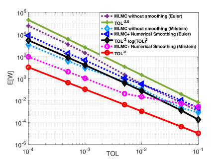
Figure 4.3: Digital option under the GBM model: Comparison of the numerical complexity (expected work (in seconds), $\mathrm{E}\left[W\right]$, vs tolerance, TOL, in a log–log scale) of standard MLMC, and MLMC with numerical smoothing, combined with the Euler or Milstein schemes. When both Euler and Milstein schemes, MLMC combined with numerical smoothing outperforms standard MLMC, and achieves a better numerical complexity rate. The canonical MLMC complexity (i.e., ${\mathcal{O}}\left(\text{TOL}^{-2}\right)$) is obtained when using the Milstein scheme with our approach.

Remark 4.3.

Notably, for the particular case of the GBM dynamics, a decaying variance of $P_{\ell}$ in the top left plots presented in Figures 1(b) and 2(b) is expected because we use a Brownian bridge for path construction. Additionally, the integrand only depends on the terminal value of the Brownian bridge, which has a variance scale of the order $\Delta t$. Therefore, for this particular case, we expect the numerical complexity of the MC method with smoothing to be on the order of ${\mathcal{O}}\left(\text{TOL}^{-2}\right)$. This feature does not hold anymore for the Heston model, as demonstrated later.

4.1.2 Pricing Digital Option/Computing Probability under the Heston Model

We consider the Heston model (4.2), with the parameters: $T=1$, $X_{0}=K=100$, $v_{0}=0.04$, $\mu=0$, $\rho=-0.9$, $\zeta=1$, $\xi=0.1$, and $\theta=0.0025$ (these parameters do not satisfy the Feller condition, i.e., $\xi^{2}<4\zeta\theta$). A reference solution, equal to $0.5146$, was obtained by the MC method. Table 4.2 summarizes the results for approximating the probability/digital option price defined by (4.3) using Euler–Maruyama scheme. Figures 4.4 and 4.5 present more details. From these figures and Table 4.2, we obtain the following results:

1. The kurtosis substantially reduces at the finest level, $\kappa_{L}$, of MLMC when using numerical smoothing. The kurtosis is bounded and reduced by a factor of $>27$.

2. Numerical smoothing considerably reduces the variance of coupled levels in MLMC. Further, it improves the variance decay rate from $\beta=1/2$ to $\beta=1$, implying an improvement in the MLMC numerical complexity from ${\mathcal{O}}\left(\text{TOL}^{-2.5}\right)$ to ${\mathcal{O}}\left(\text{TOL}^{-2}\left(\log(\text{TOL})\right)^{2}\right)$.

Method	$\kappa_{L}$	$\alpha$	$\beta$	$\gamma$	Numerical complexity
MLMC without smoothing (FT Euler–Maruyama)	$350$	$1$	$1/2$	$1$	${\mathcal{O}}\left(\text{TOL}^{-2.5}\right)$
MLMC with numerical smoothing (FT Euler–Maruyama)	$9$	$1$	$1$	$1$	${\mathcal{O}}\left(\text{TOL}^{-2}\log(\text{TOL})^{2}\right)$

Table 4.2: Digital option/probability under the Heston model: Summary of the MLMC numerical results, which correspond to Figures 4.4 and 4.5.

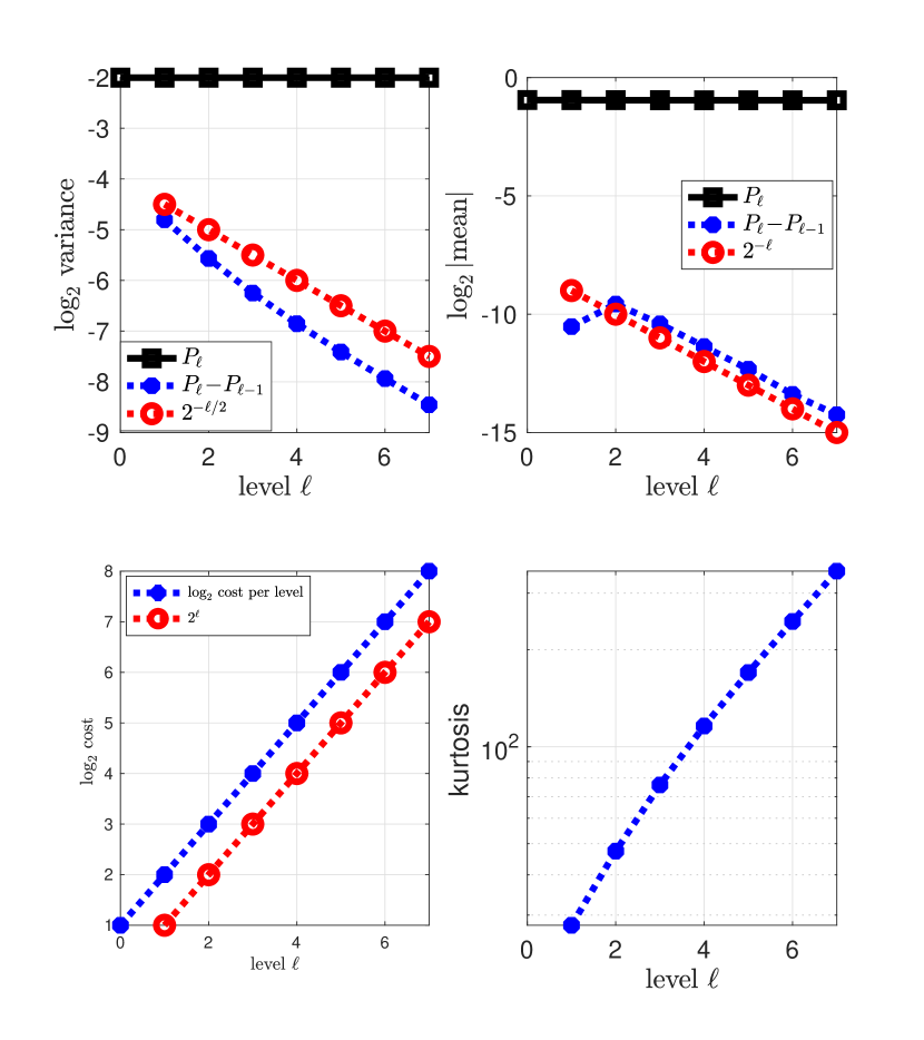
(a) Without smoothing.

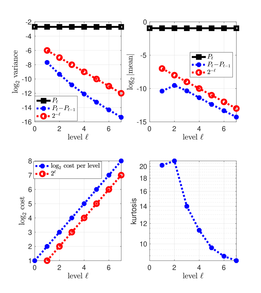
(b) With numerical smoothing $(\text{TOL}_{\text{Newton},\ell}=10^{-3},M_{\text{Lag},\ell}=32)$

Figure 4.4: Probability/Digital option under Heston: Convergence plots for MLMC combined with the Euler–Maruyama scheme and FT.

Figure 4.5: Digital option/probability under the Heston model: Comparison of the numerical complexity (expected work (in seconds), $\mathrm{E}\left[W\right]$, vs tolerance, TOL, in a log–log scale) of the standard MLMC and MLMC with numerical smoothing. MLMC combined with numerical smoothing outperforms standard MLMC and achieves a better numerical complexity rate.

Remark 4.4 (On Milstein scheme for the Heston model).

In this work, we present the results of using the Milstein scheme with MLMC for a scalar SDE in the context of the GBM example. However, when applied to multidimensional problems such as the Heston model, the Milstein scheme requires the simulation of expensive iterated Itô integrals, known as the Lévy areas. In future work, we plan to explore the potential of combining our numerical smoothing idea with the antithetic MLMC estimator proposed in [26] to address this issue and improve overall performance.

4.2 Density Approximation

4.2.1 Density Approximation under the GBM Model

We compute the density $\rho_{X(T)}$, given by (2.12), at $u=1$ for the GBM example with the parameters: $X_{0}=1$, $T=1$, and $\sigma=0.2$. In this case, $X(T)$ is lognormally distributed with parameters $-\sigma^{2}/2$ and $\sigma$. Table 4.3 summarizes the results of MLMC combined with numerical smoothing.

Method	$\kappa_{L}$	$\alpha$	$\beta$	$\gamma$	Numerical complexity
MLMC combined with numerical smoothing (Euler)	$3$	$1$	$1$	$1$	${\mathcal{O}}\left(\text{TOL}^{-2}\left(\log(\text{TOL})\right)^{2}\right)$
MLMC combined with numerical smoothing (Milstein)	$3$	$1$	$2$	$1$	${\mathcal{O}}\left(\text{TOL}^{-2}\right)$

Table 4.3: Density of GBM: Summary of the MLMC results for computing the density $\rho_{X(T)}$ at $u=1$, where $X$ follows the GBM dynamics. These results correspond to Figures 6(a) and 4.7.

Figure 6(a) depicts the detailed convergence, where we verify that the kurtosis is bounded and that the variance decay rate is on order $1$ for the Euler–Maruyama and $2$ for the Milstein scheme, resulting in a numerical complexity of the MLMC estimator to be on the order of ${\mathcal{O}}\left(\text{TOL}^{-2}\left(\log(\text{TOL})\right)^{2}\right)$ for Euler–Maruyama and ${\mathcal{O}}\left(\text{TOL}^{-2}\right)$ for Milstein scheme, as confirmed in Figure 4.7.

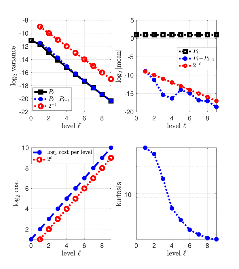
(a) Euler–Maruyama

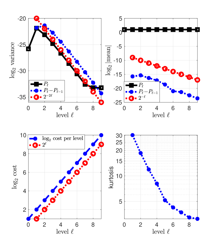
(b) Milstein

Figure 4.6: Density of GBM: Convergence plots for MLMC with numerical smoothing $(\text{TOL}_{\text{Newton},\ell}=10^{-4})$ for computing the density $\rho_{X(T)}$ at $u=1$, where $X$ follows the GBM dynamics. Remark 4.3 also holds in this example.

Figure 4.7: Density of GBM: Numerical complexity of MLMC with numerical smoothing for computing the density $\rho_{X(T)}$ at $u=1$, where $X$ follows the GBM dynamics. The canonical MLMC complexity (i.e., ${\mathcal{O}}\left(\text{TOL}^{-2}\right)$) is obtained when using the Milstein scheme with our approach.

4.2.2 Asset Price and Joint Densities Approximation under the Heston Model

We compute the density $\rho_{X(T)}$, given by (2.12), at $u=1$ such that $X$ is a Heston asset (4.2), with parameters: $X_{0}=1$, $v_{0}=0.04$, $\mu=0$, $\rho=-0.9$, $\zeta=1$, $\xi=0.1$, and $\theta=0.0025$. A reference solution, equal to $2.4475$, was obtained by applying the fractional Fourier transform to the characteristic function. Table 4.4 summarizes the results. Figure 8(a) details the convergence results for the MLMC estimator combined with the numerical smoothing, using the FT Euler–Maruyama scheme. This figure verifies that the kurtosis is bounded and that the variance decay rate is of order $1$ for the Euler–Maruyama scheme, resulting in a numerical complexity of the MLMC estimator in the order of ${\mathcal{O}}\left(\text{TOL}^{-2}\left(\log(\text{TOL})\right)^{2}\right)$, as confirmed in Figure 4.9.

Method	$\kappa_{L}$	$\alpha$	$\beta$	$\gamma$	Numerical complexity
MLMC with numerical smoothing + (FT Euler–Maruyama)	$9$	$1$	$1$	$1$	${\mathcal{O}}\left(\text{TOL}^{-2}\left(\log(\text{TOL})\right)^{2}\right)$

Table 4.4: Density of Heston: Summary of the MLMC numerical results observed for computing the density $\rho_{X(T)}$ at $u=1$, where $X$ follows the Heston dynamics. These results correspond to Figures 4.8 and 4.9.

(a) Asset price density

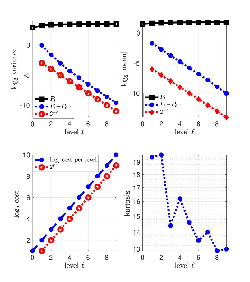
(b) Joint density

Figure 4.8: Density of Heston: Convergence plots for MLMC with numerical smoothing $(\text{TOL}_{\text{Newton},\ell}=10^{-2})$ combined with the FT scheme, for computing the asset price density $\rho_{X(T)}$ at $u=1$ and the joint density $\rho_{X(T),v(T)}$ at $u=1$ and $v=0.04$.

With the same model parameters, we compute the joint density $\rho_{X(T),v(T)}$ at $u=1$ and $v=0.04$. A reference solution was obtained by the kernel density estimator. Figure 8(b) presents the detailed convergence results for the MLMC estimator combined with the numerical smoothing, using the FT Euler–Maruyama scheme. This figure verifies that the kurtosis is bounded and that the variance decay rate is of order $1$ for the Euler–Maruyama scheme, resulting in a numerical complexity of the MLMC estimator of the order of ${\mathcal{O}}\left(\text{TOL}^{-2}\left(\log(\text{TOL})\right)^{2}\right)$.

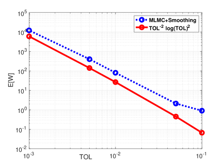
Figure 4.9: Asset price density of Heston: Numerical complexity (expected work, $\mathrm{E}\left[W\right]$ (in seconds), vs tolerance, TOL) of MLMC with numerical smoothing for computing the density $\rho_{X(T)}$ at $u=1$, where $X$ follows the Heston dynamics.

Acknowledgments C. Bayer gratefully acknowledges funding by the Deutsche Forschungsgemeinschaft (DFG, German Research Foundation) under Germany ’s Excellence Strategy – The Berlin Mathematics Research Center MATH+ (EXC-2046/1, project ID: 390685689). This publication is based on work supported by the King Abdullah University of Science and Technology (KAUST) Office of Sponsored Research (OSR) under Award No. OSR-2019-CRG8-4033 and the Alexander von Humboldt Foundation. The authors are also very grateful to the anonymous referees for their valuable feedback that greatly contributed to shape the final version of the paper.

Appendix A Additional Results for the Proofs of Theorems 3.7 and 3.8

This section states and proves the additional theoretical results for the proofs of Theorems 3.7 and 3.8 in Section 3.2. We use the same notation as in Section 3.2.

Proposition A.1 (Vanishing boundary terms).

Assume that $a(\cdot)$ and $b(\cdot)$ in (2.5) satisfy Assumption 3.5, and that Assumption B.2 holds. Then

(A.1) $$\underset{\left\lvert y\right\rvert\rightarrow\infty}{\lim}f(y;B_{\ell}):=E\left[\left(e_{\ell}(T;y,B_{\ell})\;\rho_{1}(y)\int_{0}^{1}g(z(\theta,y;B_{\ell}))\left(\partial_{y}z(\theta,y;B_{\ell})\right)^{-1}d\theta\right)^{2}\right]=0.$$

Proof.

We have $g(\cdot)$ is bounded and by Assumption B.2, we have also $\left(\partial_{y}z(\theta;y,B_{\ell})\right)^{-1}$ is bounded in moments (similar to what we showed for (3.18) in the proof of Thorem 3.7). Consequently, we need to show that $\underset{\left\lvert y\right\rvert\rightarrow\infty}{\lim}E\left[e^{2}_{\ell}(T;y,B_{\ell})\;\right]\rho_{1}(y)=0$.

First observe that $E\left[e^{2}_{\ell}(T;y,B_{\ell})\right]\leq E\left[\overline{X}^{2}_{\ell}(T;y,B_{\ell})\right]+E\left[\overline{X}^{2}_{\ell-1}(T;y,B_{\ell})\right]$. Therefore, to conclude our target result, we just need to get a bound on $E\left[\overline{X}^{2}_{\ell}(T;y,B_{\ell})\right]$. For that we will use the discrete version of Grönwall’s inequality and show that, for the time grid at level $\ell$: $0=t^{\ell}_{0}<\ldots<t_{n}^{\ell}<\dots<t^{\ell}_{N_{\ell}}$, we have $E\left[\overline{X}^{2}_{\ell}(t_{n+1}^{\ell})\right]\leq(1+K\Delta t_{n}^{\ell})E\left[\overline{X}^{2}_{\ell}(t_{n}^{\ell})\right]+A_{n}$, to conclude that $E\left[\overline{X}^{2}_{\ell}(t_{n}^{\ell})\right]\leq\overline{X}^{2}_{\ell}(0)e^{Kt^{\ell}_{n}}+\sum_{i=0}^{n-1}A_{i}e^{Kt_{i}^{\ell}}$.

We recall that $\overline{X}_{\ell}(t_{n+1}^{\ell})=\overline{X}_{\ell}(t_{n}^{\ell})+a(\overline{X}_{\ell}(t_{n}^{\ell}))\Delta t_{\ell}+b(\overline{X}_{\ell}(t_{n}^{\ell}))\left(\frac{y}{\sqrt{T}}\Delta t^{\ell}+\Delta B_{n,\ell}\right)$. Therefore, using Assumption 3.5, we obtain

$$E\left[\overline{X}^{2}_{\ell}(t_{n+1}^{\ell})\right]= E\left[\overline{X}^{2}_{\ell}(t_{n}^{\ell})\right]+E\left[b^{2}(\overline{X}_{\ell}(t_{n}^{\ell}))\left(\Delta B_{n,\ell}\right)^{2}\right]+E\left[\left(a(\overline{X}_{\ell}(t_{n}^{\ell}))+\frac{y}{\sqrt{T}}b(\overline{X}_{\ell}(t_{n}^{\ell}))\right)^{2}\right]\Delta t_{\ell}^{2}$$

$$+2E\left[\overline{X}_{\ell}(t_{n}^{\ell})\left(a(\overline{X}_{\ell}(t_{n}^{\ell}))+\frac{y}{\sqrt{T}}b(\overline{X}_{\ell}(t_{n}^{\ell}))\right)\right]\Delta t_{\ell}+2E\left[\overline{X}_{\ell}(t_{n}^{\ell})b(\overline{X}_{\ell}(t_{n}^{\ell}))\Delta B_{n,\ell}\right]$$

$$+2E\left[\left(a(\overline{X}_{\ell}(t_{n}^{\ell}))+\frac{y}{\sqrt{T}}b(\overline{X}_{\ell}(t_{n}^{\ell}))\right)b(\overline{X}_{\ell}(t_{n}^{\ell}))\Delta B_{n,\ell}\right]\Delta t_{\ell}$$

$$\leq E\left[\overline{X}^{2}_{\ell}(t_{n}^{\ell})\right]+C_{1}^{2}\underset{=\Delta t_{\ell}-\frac{\Delta t_{\ell}^{2}}{T}}{\underbrace{E\left[\left(\Delta B_{n,\ell}\right)^{2}\right]}}+(1+\Delta t_{\ell})\Delta t_{\ell}(C_{2}^{2}+C_{1}^{2}\frac{y^{2}}{T}+2C_{1}C_{2}\frac{y}{\sqrt{T}})+\Delta t_{\ell}E\left[\overline{X}^{2}_{\ell}(t_{n}^{\ell})\right]+E\left[\overline{X}^{2}_{\ell}(t_{n}^{\ell})\right]$$

$$+C_{1}^{2}\underset{=\Delta t_{\ell}-\frac{\Delta t_{\ell}^{2}}{T}}{\underbrace{E\left[\left(\Delta B_{n,\ell}\right)^{2}\right]}}+2(C_{1}C_{2}+C_{1}^{2}\frac{y}{\sqrt{T}})\Delta t_{\ell}\underset{=0}{\underbrace{E\left[\Delta B_{n,\ell}\right]}}$$

$$=E\left[\overline{X}^{2}_{\ell}(t_{n}^{\ell})\right]\left(2+\Delta t_{\ell}\right)+\underset{=A_{n}(y)}{\underbrace{\left(\left(1+\Delta t_{\ell}\right)\Delta t_{\ell}\left(\frac{C_{1}^{2}}{T}y^{2}+2\frac{C_{1}C_{2}}{\sqrt{T}}y\right)+\Delta t_{\ell}\left(2C_{1}^{2}\left(1-\frac{\Delta t_{\ell}}{T}\right)+C_{2}^{2}\left(1+\Delta t_{\ell}\right)\right)\right)}}$$

(A.2) $$=2(1+\frac{\Delta t_{n}^{\ell}}{2})E\left[\overline{X}^{2}_{\ell}(t_{n}^{\ell})\right]+A(y).$$

Using (A) and the discrete version of Grönwall’s inequality, we conclude that

(A.3) $$E\left[\overline{X}^{2}_{\ell}(T)\right]\leq 2^{N_{\ell}}\overline{X}^{2}_{\ell}(0)e^{T/2}+A(y)\sum_{i=0}^{N_{\ell}}2^{i}e^{t_{i}^{\ell}/2}.$$

Since $A(y)$ is quadratic in $y$, we conclude that, for a given $\Delta t_{\ell}$, $\underset{\left\lvert y\right\rvert\rightarrow\infty}{\lim}E\left[e^{2}_{\ell}(T;y,B_{\ell})\;\right]\rho_{1}(y)=0$. ∎

Remark A.2 (Relaxing Assumption 3.5 in the proof of Proposition A.1 and Theorems 3.7 and 3.8).

In the above proof, we showed that for a given $\Delta t_{\ell}$, we obtain $\underset{\left\lvert y\right\rvert\rightarrow\infty}{\lim}E\left[e^{2}_{\ell}(T;y,B_{\ell})\;\right]\rho_{1}(y)=0$. Therefore the growth observed in the bound (A.3) w.r.t $N_{\ell}$ is not problematic for the sake of that proof. However, we emphasise that a better bound can be derived for small $\Delta t_{\ell}$ using the following arguments and sketch of proof:

The three terms $E\left[\left(a(\overline{X}_{\ell}(t_{n}^{\ell}))+\frac{y}{\sqrt{T}}b(\overline{X}_{\ell}(t_{n}^{\ell}))\right)b(\overline{X}_{\ell}(t_{n}^{\ell}))\Delta B_{n,\ell}\right]$, $E\left[\overline{X}_{\ell}(t_{n}^{\ell})b(\overline{X}_{\ell}(t_{n}^{\ell}))\Delta B_{n,\ell}\right]$, and $E\left[b^{2}(\overline{X}_{\ell}(t_{n}^{\ell}))\left(\Delta B_{n,\ell}\right)^{2}\right]$ in (A) can be represented as $E\left[F(\{\Delta B_{m,\ell}\}_{m=1,m\neq n}^{N_{\ell}},\Delta B_{n,\ell})\left(\Delta B_{n,\ell}\right)^{k}\right]$, where $k=1,2$ and $F(\{\Delta B_{m,\ell}\}_{m=1,m\neq n}^{N_{\ell}},\Delta B_{n,\ell})$ is a function of $\Delta B_{n,\ell}$ and the remaing Brownian bridge increments $\{\Delta B_{m,\ell}\}_{m=1,m\neq n}^{N_{\ell}}$. For $\Delta t_{\ell}\rightarrow 0$, applying Taylor expansion for $F(\cdot)$ around $\Delta B_{n,\ell}$ implies that

$$E\left[F(\{\Delta B_{m,\ell}\}_{m=1,m\neq n}^{N_{\ell}},\Delta B_{n,\ell})\left(\Delta B_{n,\ell}\right)^{k}\right]$$

$$=E\left[\left(F(\{\Delta B_{m,\ell}\}_{m=1,m\neq n}^{N_{\ell}},0)+F^{\prime}(\{\Delta B_{m,\ell}\}_{m=1,m\neq n}^{N_{\ell}},0)\Delta B_{n,\ell}+\text{h.o.t}\right)\left(\Delta B_{n,\ell}\right)^{k}\right]$$

$$=E\left[F(\{\Delta B_{m,\ell}\}_{m=1,m\neq n}^{N_{\ell}},0)\right]E\left[\left(\Delta B_{n,\ell}\right)^{k}\right]+E\left[F^{\prime}(\{\Delta B_{m,\ell}\}_{m=1,m\neq n}^{N_{\ell}},0)\right]E\left[\left(\Delta B_{n,\ell}\right)^{k+1}\right]+\text{h.o.t}$$

(A.4) $$=E\left[F^{(2-k)}(\{\Delta B_{m,\ell}\}_{m=1,m\neq n}^{N_{\ell}},0)\right]\underset{=\Delta t_{\ell}-\frac{\Delta t_{\ell}^{2}}{T}\overset{\Delta t_{\ell}\rightarrow 0}{\longrightarrow}0}{\underbrace{E\left[\left(\Delta B_{n,\ell}\right)^{2}\right]}}+\text{h.o.t},\>k=1,2.$$

In this case we can relax Assumption 3.5 and use Assumption 3.2 instead, and we obtain

$$E\left[\overline{X}^{2}_{\ell}(t_{n+1}^{\ell})\right]= E\left[\overline{X}^{2}_{\ell}(t_{n}^{\ell})\right]+E\left[b^{2}(\overline{X}_{\ell}(t_{n}^{\ell}))\left(\Delta B_{n,\ell}\right)^{2}\right]+E\left[\left(a(\overline{X}_{\ell}(t_{n}^{\ell}))+\frac{y}{\sqrt{T}}b(\overline{X}_{\ell}(t_{n}^{\ell}))\right)^{2}\right]\Delta t_{\ell}^{2}$$

$$+2E\left[\overline{X}_{\ell}(t_{n}^{\ell})\left(a(\overline{X}_{\ell}(t_{n}^{\ell}))+\frac{y}{\sqrt{T}}b(\overline{X}_{\ell}(t_{n}^{\ell}))\right)\right]\Delta t_{\ell}+2E\left[\overline{X}_{\ell}(t_{n}^{\ell})b(\overline{X}_{\ell}(t_{n}^{\ell}))\Delta B_{n,\ell}\right]$$

$$+2E\left[\left(a(\overline{X}_{\ell}(t_{n}^{\ell}))+\frac{y}{\sqrt{T}}b(\overline{X}_{\ell}(t_{n}^{\ell}))\right)b(\overline{X}_{\ell}(t_{n}^{\ell}))\Delta B_{n,\ell}\right]\Delta t_{\ell}$$

$$\underset{\Delta t_{\ell}\rightarrow 0}{\lessapprox}E\left[\overline{X}^{2}_{\ell}(t_{n}^{\ell})\right]\left(1+C^{2}\Delta t_{\ell}^{2}(1+\frac{y}{\sqrt{T}})^{2}+2C\Delta t_{\ell}(1+\frac{y}{\sqrt{T}})\right)+\text{h.o.t}$$

$$=E\left[\overline{X}^{2}_{\ell}(t_{n}^{\ell})\right]\left(1+C^{2}\Delta t_{\ell}^{2}(1+\frac{y}{\sqrt{T}})^{2}+2C\Delta t_{\ell}(1+\frac{y}{\sqrt{T}})\right)+\text{h.o.t}$$

(A.5) $$=(1+K(y)\Delta t_{n}^{\ell})E\left[\overline{X}^{2}_{\ell}(t_{n}^{\ell})\right]+\text{h.o.t},$$

with $K(y)=C^{2}\frac{\Delta t_{\ell}^{2}}{T}y^{2}+2y\left(C^{2}\frac{\Delta t_{\ell}}{\sqrt{T}}+\frac{C}{\sqrt{T}}\right)\Delta t_{\ell}+\Delta t_{\ell}(C^{2}\Delta t_{\ell}+2C)$.

Using (A) and the discrete version of Grönwall’s inequality, we conclude that

$$E\left[\overline{X}^{2}_{\ell}(T)\right]\leq\overline{X}^{2}_{\ell}(0)e^{K(y)T},$$

and that for sufficiently small $\Delta t_{\ell}\rightarrow 0$, we obtain $\underset{\left\lvert y\right\rvert\rightarrow\infty}{\lim}E\left[e^{2}_{\ell}(T;y,B_{\ell})\;\right]\rho_{1}(y)=0$.

Lemma A.3 (Moments bounds for the y-derivative of the error).

Let $e_{\ell}(t;y,B_{\ell})$ as defined in (3.2), and assume that $a(\cdot)$ and $b(\cdot)$ satisfy Assumptions 3.2, 3.3, 3.4, and 3.5, and that Assumption B.1 holds. Then, we obtain for $p\geq 1$

$$\mathrm{E}\left[(\partial_{y}e_{\ell})^{2p}(T)\right]={\mathcal{O}}\left(\Delta t_{\ell}^{p}\right).$$

Proof of lemma A.3.

In the following, for ease of notation, we denote $e_{\ell}(t;y,B_{\ell})$ by $e_{\ell}(t)$. From (3.8) and (3.2) and since $(\partial_{y}e_{\ell})(0)=0$, we obtain

$$\partial_{y}e_{\ell}(t) =\int_{0}^{t}\partial_{y}\left(a(\overline{X}_{\ell}([s]_{\ell}))-a(\overline{X}_{\ell-1}([s]_{\ell-1}))\right)ds+\partial_{y}\left(\int_{0}^{t}\left(b(\overline{X}_{\ell}([s]_{\ell}))-b(\overline{X}_{\ell-1}([s]_{\ell-1}))\right)dW_{s}\right)$$

$$=\int_{0}^{t}\partial_{y}\left(a(\overline{X}_{\ell}([s]_{\ell}))-a(\overline{X}_{\ell}(s))+a(\overline{X}_{\ell}(s))-a(\overline{X}_{\ell-1}(s))+a(\overline{X}_{\ell-1}(s))-a(\overline{X}_{\ell-1}([s]_{\ell-1}))\right)ds$$

$$+\partial_{y}\left(\int_{0}^{t}\left(b(\overline{X}_{\ell}([s]_{\ell}))-b(\overline{X}_{\ell}(s))+b(\overline{X}_{\ell}(s))-b(\overline{X}_{\ell-1}(s))+b(\overline{X}_{\ell-1}(s))-b(\overline{X}_{\ell-1}([s]_{\ell-1}))\right)dW_{s}\right)$$

$$=\int_{0}^{t}\left(a^{\prime}(\overline{X}_{\ell})\partial_{y}\overline{X}_{\ell}-a^{\prime}(\overline{X}_{\ell-1})\partial_{y}\overline{X}_{\ell-1}\right)(s)\;ds+\int_{0}^{t}\left(b^{\prime}(\overline{X}_{\ell})\partial_{y}\overline{X}_{\ell}-b^{\prime}(\overline{X}_{\ell-1})\partial_{y}\overline{X}_{\ell-1}\right)(s)\;dW_{s}$$

$$+\int_{0}^{t}\left(b(\overline{X}_{\ell}(s))-b(\overline{X}_{\ell-1}(s))\right)\frac{ds}{\sqrt{T}}$$

$$+\int_{0}^{t}\partial_{y}\left(a(\overline{X}_{\ell}([s]_{\ell}))-a(\overline{X}_{\ell}(s))\right)ds+\int_{0}^{t}\partial_{y}\left(a(\overline{X}_{\ell-1}(s))-a(\overline{X}_{\ell-1}([s]_{\ell-1}))\right)ds$$

$$+\int_{0}^{t}\partial_{y}\left(b(\overline{X}_{\ell}([s]_{\ell}))-b(\overline{X}_{\ell}(s))+b(\overline{X}_{\ell-1}(s))-b(\overline{X}_{\ell-1}([s]_{\ell-1}))\right)dW_{s}$$

$$+\int_{0}^{t}\left(b(\overline{X}_{\ell}([s]_{\ell}))-b(\overline{X}_{\ell}(s))+b(\overline{X}_{\ell-1}(s))-b(\overline{X}_{\ell-1}([s]_{\ell-1}))\right)\frac{ds}{\sqrt{T}}$$

$$=\int_{0}^{t}\left(a^{\prime}(\overline{X}_{\ell})\partial_{y}e_{\ell}+\partial_{y}\overline{X}_{\ell-1}\left(\int_{0}^{1}a^{\prime\prime}(\overline{X}_{\ell-1}+\theta e_{\ell})d\theta\right)e_{\ell}\right)(s)\;ds$$

$$+\int_{0}^{t}\left(\int_{0}^{1}b^{\prime}(\overline{X}_{\ell-1}+\theta e_{\ell})d\theta\right)(s)e_{\ell}(s)\;\frac{ds}{\sqrt{T}}$$

$$+\int_{0}^{t}\left(b^{\prime}(\overline{X}_{\ell})\partial_{y}e_{\ell}+\partial_{y}\overline{X}_{\ell-1}\left(\int_{0}^{1}b^{\prime\prime}(\overline{X}_{\ell-1}+\theta e_{\ell})d\theta\right)e_{\ell}\right)(s)\;dW_{s}$$

$$+\int_{0}^{t}\partial_{y}\left(a(\overline{X}_{\ell}([s]_{\ell}))-a(\overline{X}_{\ell}(s))\right)ds+\int_{0}^{t}\partial_{y}\left(a(\overline{X}_{\ell-1}(s))-a(\overline{X}_{\ell-1}([s]_{\ell-1}))\right)ds$$

$$+\int_{0}^{t}\partial_{y}\left(b(\overline{X}_{\ell}([s]_{\ell}))-b(\overline{X}_{\ell}(s))+b(\overline{X}_{\ell-1}(s))-b(\overline{X}_{\ell-1}([s]_{\ell-1}))\right)dW_{s}$$

(A.6) $$+\int_{0}^{t}\left(b(\overline{X}_{\ell}([s]_{\ell}))-b(\overline{X}_{\ell}(s))+b(\overline{X}_{\ell-1}(s))-b(\overline{X}_{\ell-1}([s]_{\ell-1}))\right)\frac{ds}{\sqrt{T}}.$$

Therefore, taking expectation, we obtain

$$E\left[\left(\partial_{y}e_{\ell}(t)\right)^{2p}\right] \leq 5^{2p-1}\underset{(I)}{\underbrace{{E\left[\left(\int_{0}^{t}\left(\overline{a}^{\prime}(\overline{X}_{\ell})\partial_{y}e_{\ell}+\left(\partial_{y}\overline{X}_{\ell-1}\left(\int_{0}^{1}\overline{a}^{\prime\prime}(X_{\ell-1}+\theta e_{\ell})d\theta\right)+\int_{0}^{1}\frac{1}{\sqrt{T}}\overline{b}^{\prime}(\overline{X}_{\ell-1}+\theta e_{\ell})d\theta\right)e_{\ell}\right)ds\right)^{2p}\right]}}}$$

$$+5^{2p-1}\underset{(II)}{\underbrace{{E\left[\left(\int_{0}^{t}\left(\overline{b}^{\prime}(\overline{X}_{\ell})\partial_{y}e_{\ell}+\partial_{y}\overline{X}_{\ell-1}\left(\int_{0}^{1}\overline{b}^{\prime\prime}(\overline{X}_{\ell-1}+\theta e_{\ell})d\theta\right)e_{\ell}\right)dWs\right)^{2p}\right]}}}$$

$$+5^{2p-1}\underset{(III)}{\underbrace{{E\left[\left(\int_{0}^{t}\partial_{y}\left(a(\overline{X}_{\ell}([s]_{\ell}))-a(\overline{X}_{\ell}(s))\right)ds+\int_{0}^{t}\partial_{y}\left(a(\overline{X}_{\ell-1}(s))-a(\overline{X}_{\ell-1}([s]_{\ell-1}))\right)ds\right)^{2p}\right]}}}$$

$$+5^{2p-1}\underset{(IV)}{\underbrace{{E\left[\left(\int_{0}^{t}\partial_{y}\left(b(\overline{X}_{\ell}([s]_{\ell}))-b(\overline{X}_{\ell}(s))+b(\overline{X}_{\ell-1}(s))-b(\overline{X}_{\ell-1}([s]_{\ell-1}))\right)dW_{s}\right)^{2p}\right]}}}$$

(A.7) $$+5^{2p-1}\underset{(V)}{\underbrace{{E\left[\left(\int_{0}^{t}\left(b(\overline{X}_{\ell}([s]_{\ell}))-b(\overline{X}_{\ell}(s))+b(\overline{X}_{\ell-1}(s))-b(\overline{X}_{\ell-1}([s]_{\ell-1}))\right)\frac{ds}{\sqrt{T}}\right)^{2p}\right]}}}$$

The idea now is to show that $E\left[\left(\partial_{y}e_{\ell}(t)\right)^{2p}\right]\leq K\int_{0}^{t}E\left[\left(\partial_{y}e_{\ell}(s)\right)^{2p}\right]ds+A$, where $0<K<\infty$ and $A={\mathcal{O}}\left(\Delta t_{\ell}^{p}\right)$, then, using Grönwall’s inequality we get the result.

Let $p_{1},q_{1},p_{5},q_{5}\in(1,+\infty)$ with $\frac{1}{p_{1}}+\frac{1}{q_{1}}=1$ and $\frac{1}{p_{5}}+\frac{1}{q_{5}}=1$ such that $p_{5}p/p_{1}\leq 1$. Then using the Hölder, Burkholder-Davis-Gundy and Jensen inequalities, we obtain for (II) in (A)

$$(II) \leq 2^{p-1}\left(E\left[\left(\int_{0}^{t}\overline{b}^{\prime}(\overline{X}_{\ell})\partial_{y}e_{\ell}dWs\right)^{2p}\right]+E\left[\left(\int_{0}^{t}\partial_{y}\overline{X}_{\ell-1}\left(\int_{0}^{1}\overline{b}^{\prime\prime}(\overline{X}_{\ell-1}+\theta e_{\ell})d\theta\right)e_{\ell}dWs\right)^{2p}\right]\right)$$

$$\leq K_{1}E\left[\left(\int_{0}^{t}\left(\overline{b}^{\prime}(\overline{X}_{\ell})\partial_{y}e_{\ell}\right)^{2}ds\right)^{p}\right]+A_{1}E\left[\left(\int_{0}^{t}\left(\partial_{y}\overline{X}_{\ell-1}\left(\int_{0}^{1}\overline{b}^{\prime\prime}(\overline{X}_{\ell-1}+\theta e_{\ell})d\theta\right)e_{\ell}\right)^{2}ds\right)^{p}\right]$$

$$\leq K_{2}\;t^{p-1}E\left[\int_{0}^{t}\left(\partial_{y}e_{\ell}\right)^{2p}ds\right]$$

$$+A_{1}E\left[\left(\int_{0}^{t}\left(\partial_{y}\overline{X}_{\ell-1}\left(\int_{0}^{1}\overline{b}^{\prime\prime}(\overline{X}_{\ell-1}+\theta e_{\ell})d\theta\right)\right)^{2q_{1}}ds\right)^{p/q_{1}}\times\left(\int_{0}^{t}\left(e_{\ell}\right)^{2p_{1}}ds\right)^{p/p_{1}}\right]$$

$$\leq K_{2}\;t^{p-1}E\left[\int_{0}^{t}\left(\partial_{y}e_{\ell}\right)^{2p}ds\right]$$

$$+A_{1}E\left[\left(\int_{0}^{t}\left(\partial_{y}\overline{X}_{\ell-1}\left(\int_{0}^{1}\overline{b}^{\prime\prime}(\overline{X}_{\ell-1}+\theta e_{\ell})d\theta\right)\right)^{2q_{1}}ds\right)^{q_{5}p/q_{1}}\right]^{1/q_{5}}\times E\left[\left(\int_{0}^{t}\left(e_{\ell}\right)^{2p_{1}}ds\right)^{p_{5}p/p_{1}}\right]^{1/p_{5}}$$

$$\leq K_{2}\;t^{p-1}E\left[\int_{0}^{t}\left(\partial_{y}e_{\ell}\right)^{2p}ds\right]$$

(A.8) $$+A_{1}\underset{<\infty}{\underbrace{E\left[\left(\int_{0}^{t}\left(\partial_{y}\overline{X}_{\ell-1}\left(\int_{0}^{1}\overline{b}^{\prime\prime}(\overline{X}_{\ell-1}+\theta e_{\ell})d\theta\right)\right)^{2q_{1}}ds\right)^{q_{5}p/q_{1}}\right]^{1/q_{5}}}}\times\underset{{\mathcal{O}}\left(\Delta t_{\ell}^{p}\right)}{\underbrace{E\left[\left(\int_{0}^{t}\left(e_{\ell}\right)^{2p_{1}}ds\right)\right]^{p/p_{1}}}}$$

where we used (3.14), Assumption B.1, and that $b^{\prime}(X_{\ell})$ is uniformly bounded due to Assumption 3.2, to get (A).

For term (I) in (A), using Hölder’s inequality ($p_{2},q_{2},p_{6},q_{6}\in(1,+\infty)$ with $\frac{1}{p_{2}}+\frac{1}{q_{2}}=1$ and $\frac{1}{p_{6}}+\frac{1}{q_{6}}=1$) and $2p_{6}p/p_{2}\leq 1$ to use Jensen’s inequality, we obtain

$$(I) \leq 2^{p-1}E\left[\left(\int_{0}^{t}\overline{a}^{\prime}(\overline{X}_{\ell})\partial_{y}e_{\ell}ds\right)^{2p}\right]$$

$$+2^{p-1}E\left[\left(\int_{0}^{t}\left(\partial_{y}\overline{X}_{\ell-1}\left(\int_{0}^{1}\overline{a}^{\prime\prime}(\overline{X}_{\ell-1}+\theta e_{\ell})d\theta\right)+\int_{0}^{1}\frac{1}{\sqrt{T}}\overline{b}^{\prime}(\overline{X}_{\ell-1}+\theta e_{\ell})d\theta\right)e_{\ell}ds\right)^{2p}\right]$$

$$\leq 2^{p-1}K_{3}t^{\frac{2p-1}{2p}}E\left[\int_{0}^{t}\left(\partial_{y}e_{\ell}\right)^{2p}ds\right]$$

$$+2^{p-1}E\left[\left(\int_{0}^{t}\left(\partial_{y}\overline{X}_{\ell-1}\left(\int_{0}^{1}\overline{a}^{\prime\prime}(\overline{X}_{\ell-1}+\theta e_{\ell})d\theta\right)+\int_{0}^{1}\frac{1}{\sqrt{T}}\overline{b}^{\prime}(\overline{X}_{\ell-1}+\theta e_{\ell})d\theta\right)^{q_{2}}ds\right)^{2p/q_{2}}\times\left(\int_{0}^{t}\left(e_{\ell}\right)^{p_{2}}ds\right)^{2p/p_{2}}\right]$$

$$\leq 2^{p-1}K_{3}t^{\frac{2p-1}{2p}}E\left[\int_{0}^{t}\left(\partial_{y}e_{\ell}\right)^{2p}ds\right]$$

(A.9) $$+2^{p-1}\underset{<\infty}{\underbrace{E\left[\left(\int_{0}^{t}\left(\partial_{y}\overline{X}_{\ell-1}\left(\int_{0}^{1}\overline{a}^{\prime\prime}(\overline{X}_{\ell-1}+\theta e_{\ell})d\theta\right)+\int_{0}^{1}\frac{1}{\sqrt{T}}\overline{b}^{\prime}(\overline{X}_{\ell-1}+\theta e_{\ell})d\theta\right)^{q_{2}}ds\right)^{2pq_{6}/q_{2}}\right]^{1/q_{6}}}}$$

$$\times\underset{{\mathcal{O}}\left(\Delta t_{\ell}^{p}\right)}{\underbrace{E\left[\left(\int_{0}^{t}\left(e_{\ell}\right)^{p_{2}}ds\right)^{2pp_{6}/p_{2}}\right]^{1/p_{6}}}}$$

where we used (3.14), Assumption B.1, and that $a^{\prime}(X_{\ell})$ is uniformly bounded due to Assumption 3.2, to get (A).

To end the proof, the remaining step is to show that the terms (III), (IV) and (V) in (A) are of order ${\mathcal{O}}\left(\Delta t_{\ell}^{p}\right)$. First, observe that for any $[s]_{\ell}\leq s\leq[s]_{\ell}+\Delta t_{\ell}$, using (3.8) and Assumption 3.5, we obtain for any $p\geq 1$

$$E\left[\left(\overline{X}_{\ell}([s]_{\ell})-\overline{X}_{\ell}(s)\right)^{2p}\right] =E\left[\left(a(\overline{X}([s]_{\ell}))([s]_{\ell}-s)+b(\overline{X}_{\ell}([s]_{\ell}))(W([s]_{\ell})-W(s))\right)^{2p}\right]$$

$$\leq 2^{2p-1}\underset{<\infty\text{ due to Assumption \eqref{ass: uniform boundedness of the drift and diffusion coefficients}}}{\underbrace{E\left[a(\overline{X}_{\ell}([s]_{\ell}))^{2p}\right]}}(\Delta t_{\ell})^{2p}+2^{2p-1}\underset{={\mathcal{O}}\left(\Delta t_{\ell}^{p}\right)\text{ due to Assumption \eqref{ass: uniform boundedness of the drift and diffusion coefficients}}}{\underbrace{E\left[\left(b(\overline{X}_{\ell}([s]_{\ell}))(W([s]_{\ell})-W(s))\right)^{2p}\right]}}$$

(A.10) $$={\mathcal{O}}\left(\Delta t_{\ell}^{p}\right),$$

and similarly, using (3.8) and Assumptions 3.3, 3.5, and B.1 (and Lemma B.3), we obtain

$$E\left[\left(\partial_{y}\left(\overline{X}_{\ell}([s]_{\ell})-\overline{X}_{\ell}(s)\right)\right)^{2p}\right] =E\left[\left(\partial_{y}\left(a(\overline{X}([s]_{\ell}))([s]_{\ell}-s)+b(\overline{X}_{\ell}([s]_{\ell}))(W([s]_{\ell})-W(s))\right)\right)^{2p}\right]$$

$$=E\left[\left(\partial_{y}a(\overline{X}([s]_{\ell}))([s]_{\ell}-s)+\partial_{y}b(\overline{X}_{\ell}([s]_{\ell}))(W([s]_{\ell})-W(s))+b(\overline{X}_{\ell}([s]_{\ell}))\frac{[s]_{\ell}-s}{\sqrt{T}}\right)^{2p}\right]$$

$$\leq 3^{2p-1}\underset{<\infty\text{ due to Assumptions \eqref{ass: uniform boundedness of the drift and diffusion coefficients} and \ref{ass:boundedness-derivative}}}{\underbrace{E\left[\left(a^{\prime}(\overline{X}_{\ell}([s]_{\ell}))\partial_{y}\overline{X}([s]_{\ell})\right)^{2p}\right]}}(\Delta t_{\ell})^{2p}$$

$$+3^{2p-1}\underset{={\mathcal{O}}\left(\Delta t_{\ell}^{p}\right)\text{ due to Assumptions \eqref{ass: uniform boundedness of the drift and diffusion coefficients} and \ref{ass:boundedness-derivative} }}{\underbrace{E\left[\left(b^{\prime}(\overline{X}_{\ell}([s]_{\ell}))\partial_{y}\overline{X}([s]_{\ell})(W([s]_{\ell})-W(s))\right)^{2p}\right]}}$$

$$\leq 3^{2p-1}T^{-p}\underset{<\infty\text{ due to Assumption \eqref{ass: uniform boundedness of first order derivatives}}}{\underbrace{E\left[\left(b(\overline{X}_{\ell}([s]_{\ell})\right)^{2p}\right]}}(\Delta t_{\ell})^{2p}$$

(A.11) $$={\mathcal{O}}\left(\Delta t_{\ell}^{p}\right),$$

For the term (III) in (A), we focus on the first integral contribution, and the analysis follows similarly for the second one. Following similar steps as in (A), i.e., using Hölder’s inequality ($p_{2},q_{2},p_{6},q_{6}\in(1,+\infty)$ with $\frac{1}{p_{2}}+\frac{1}{q_{2}}=1$ and $\frac{1}{p_{6}}+\frac{1}{q_{6}}=1$) and $2p_{6}p/p_{2}\leq 1$ to use Jensen’s inequality, we obtain

$$E\left[\left(\int_{0}^{t}\partial_{y}\left(a(\overline{X}_{\ell}([s]_{\ell}))-a(\overline{X}_{\ell}(s))\right)ds\right)^{2p}\right]$$

$$\leq 2^{2p-1}E\left[\left(\int_{0}^{t}a^{\prime}(\overline{X}_{\ell}([s]_{\ell}))\left(\partial_{y}\left(\overline{X}_{\ell}([s]_{\ell})-\overline{X}_{\ell}(s)\right)\right)ds\right)^{2p}\right]$$

$$+2^{2p-1}E\left[\left(\int_{0}^{t}\partial_{y}\overline{X}_{\ell}(s)\left(a^{\prime}(\overline{X}_{\ell}([s]_{\ell}))-a^{\prime}(\overline{X}_{\ell}(s))\right)ds\right)^{2p}\right]$$

$$\leq 2^{2p-1}K_{4}t^{\frac{2p-1}{2p}}\underset{{\mathcal{O}}\left(\Delta t_{\ell}^{p}\right)}{\underbrace{E\left[\int_{0}^{t}\left(\partial_{y}\left(\overline{X}_{\ell}([s]_{\ell})-\overline{X}_{\ell}(s)\right)\right)^{2p}ds\right]}}$$

(A.12) $$+2^{p-1}\underset{<\infty}{\underbrace{E\left[\left(\int_{0}^{t}\left(\partial_{y}\overline{X}_{\ell}\right)^{q_{2}}ds\right)^{2pq_{6}/q_{2}}\right]^{1/q_{6}}}}\times\underset{{\mathcal{O}}\left(\Delta t_{\ell}^{p}\right)}{\underbrace{E\left[\left(\int_{0}^{t}\left(a^{\prime}(\overline{X}_{\ell}([s]_{\ell}))-a^{\prime}(\overline{X}_{\ell}(s))\right)^{p_{2}}ds\right)^{2pp_{6}/p_{2}}\right]^{1/p_{6}}}},$$

where we used (A), (A), and that $a^{\prime}(\cdot)$ is Lipchitz due to Assumption 3.4 to get the bound for the last term in (A).

For the term (IV) in (A), we focus on the first integral contribution, and the analysis follows similarly for the second one. We follow similar steps as in (A). Let $p_{1},q_{1},p_{5},q_{5}\in(1,+\infty)$ with $\frac{1}{p_{1}}+\frac{1}{q_{1}}=1$ and $\frac{1}{p_{5}}+\frac{1}{q_{5}}=1$ such that $p_{5}p/p_{1}\leq 1$. Then using the Hölder, Burkholder-Davis-Gundy and Jensen inequalities, we obtain

$$E\left[\left(\int_{0}^{t}\partial_{y}\left(b(\overline{X}_{\ell}([s]_{\ell}))-b(\overline{X}_{\ell}(s))\right)dW_{s}\right)^{2p}\right]$$

$$\leq 2^{2p-1}E\left[\left(\int_{0}^{t}b^{\prime}(\overline{X}_{\ell}([s]_{\ell}))\left(\partial_{y}\left(\overline{X}_{\ell}([s]_{\ell}))-\overline{X}_{\ell}(s))\right)\right)dW_{s}\right)^{2p}\right]$$

$$+2^{2p-1}E\left[\left(\int_{0}^{t}\partial_{y}\overline{X}_{\ell}(s)\left(b^{\prime}(\overline{X}_{\ell}([s]_{\ell}))-b^{\prime}(\overline{X}_{\ell}(s))\right)dW_{s}\right)^{2p}\right]$$

$$\leq K_{5}\;t^{p-1}\underset{{\mathcal{O}}\left(\Delta t_{\ell}^{p}\right)}{\underbrace{E\left[\int_{0}^{t}\left(\partial_{y}\left(\overline{X}_{\ell}([s]_{\ell}))-\overline{X}_{\ell}(s))\right)\right)^{2p}ds\right]}}$$

(A.13) $$+K_{6}\underset{<\infty}{\underbrace{E\left[\left(\int_{0}^{t}\left(\partial_{y}\overline{X}_{\ell}\right)^{2q_{1}}ds\right)^{q_{5}p/q_{1}}\right]^{1/q_{5}}}}\times\underset{{\mathcal{O}}\left(\Delta t_{\ell}^{p}\right)}{\underbrace{E\left[\left(\int_{0}^{t}\left(b^{\prime}(\overline{X}_{\ell}([s]_{\ell}))-b^{\prime}(\overline{X}_{\ell}(s))\right)^{2p_{1}}ds\right)\right]^{p/p_{1}}}},$$

where we used (A), (A), and that $b^{\prime}(\cdot)$ is Lipchitz due to Assumption 3.4 to get the bound for the last term in (A).

For the term (V) in (A), we focus on the first integral contribution, and the analysis follows similarly for the second one. Using Hölder’s inequality, (A), and that $b(\cdot)$ is Lipchitz due to Assumption 3.4, we obtain

(A.14) $$E\left[\left(\int_{0}^{t}\left(b(\overline{X}_{\ell}([s]_{\ell}))-b(\overline{X}_{\ell}(s))\right)\frac{ds}{\sqrt{T}}\right)^{2p}\right]={\mathcal{O}}\left(\Delta t_{\ell}^{p}\right)$$

∎

Remark A.4 (Extending Lemma A.3 for higher order derivatives).

It is easy to extend the result of Lemma A.3 for higher order terms, that is $\mathrm{E}\left[(\partial^{k}_{y}e_{\ell})^{2p}\right]={\mathcal{O}}\left(\Delta t_{\ell}^{p}\right)$ for $p\geq 1$ and $k\geq 2$. However, we need to further assume that $a(\cdot)$ and $b(\cdot)$ are of class $C^{k+1}$, besides additional uniform boundedness conditions for the higher order derivatives up to order $k$ as in the proof of Lemma A.3.

Appendix B Adapting Assumptions 3.2 and 3.3 and Lemma A.1 in [7] to our Context

This section states assumptions B.1 and B.2, and lemma B.3 which are a slightly adapted versions of Assumptions 3.2 and 3.3, and Lemma A.1 in [7]. The sufficient conditions for the assumptions to be valid are explained in Appendix B in [7].

From our construction of the approximate path at level $\ell$ using the Euler–Maruyama scheme based on the Brownian bridge construction, we have $\overline{X}_{\ell}(T)$ is a function of the rdvs $Z_{1}^{\ell}$ (corresponding to the coarsest level of the Brownian bridge $B_{\ell}$) and $\textbf{Z}^{\ell}_{-1}$ (the remaining $N_{\ell}-1$ random variables), i.e., $\overline{X}_{\ell}(T):=\overline{X}_{\ell}(T;\left(Z_{1}^{\ell},\textbf{Z}^{\ell}_{-1}\right))$. We write $y\coloneqq z^{\ell}_{1}$ and $\textbf{z}^{\ell}_{-1}$ for the (deterministic) arguments of the function $\overline{X}_{\ell}(T)$. For convenience, we will denote $\overline{X}_{\ell}(T)$ by $\overline{X}^{N_{\ell}}_{T}$ and $\overline{X}^{N_{\ell}}_{k}$ are the Euler–Maruyama increments of $\overline{X}^{N_{\ell}}_{T}$ for $0\leq k\leq{N_{\ell}}$ with $\overline{X}^{N_{\ell}}_{T}=\overline{X}^{N_{\ell}}_{N_{\ell}}$.

Assumption B.1 (Adapted version of Assumption 3.2 in [7]).

There are positive rdvs $C_{p}$ with finite moments of all orders such that

$$\forall N_{\ell}\in\mathbb{N},\ \forall k_{1},\ldots,k_{p}\in\{0,\ldots,N_{\ell}-1\}:\ \left\lvert\frac{\partial^{p}\overline{X}^{N_{\ell}}_{T}}{\partial\overline{X}^{N_{\ell}}_{k_{1}}\cdots\partial\overline{X}^{N_{\ell}}_{k_{p}}}\right\rvert\leq C_{p}\text{ a.s.}$$

In terms of notation 3.1, this means that $\frac{\partial^{p}\overline{X}^{N_{\ell}}_{T}}{\partial\overline{X}^{N_{\ell}}_{k_{1}}\cdots\partial\overline{X}^{N_{\ell}}_{k_{p}}}=\mathcal{O}(1)$.

Assumption B.2 (Adapted version of Assumption 3.3 in [7]).

For any $p\in\mathbb{N}$ we obtain

$$\left(\frac{\partial\overline{X}^{N_{\ell}}_{T}}{\partial y}\left(Z^{\ell}_{1},\textbf{Z}^{\ell}_{-1}\right)\right)^{-p}=\mathcal{O}(1).$$

Lemma B.3 (Adapted result from Lemma A.1 in [7]).

If Assumption B.1 holds, we have the following:

$$\frac{\partial\overline{X}^{N_{\ell}}_{T}}{\partial y}(Z^{\ell}_{1},\textbf{Z}^{\ell}_{-1})=\mathcal{O}(1).$$

Proof.

The proof is similar to the one for Lemma A.1 in Appendix A in [7]. ∎

References Cited

- [1] Nico Achtsis, Ronald Cools, and Dirk Nuyens. Conditional sampling for barrier option pricing under the LT method. SIAM Journal on Financial Mathematics, 4(1):327–352, 2013.
- [2] Martin Altmayer and Andreas Neuenkirch. Multilevel Monte Carlo quadrature of discontinuous payoffs in the generalized Heston model using Malliavin integration by parts. SIAM Journal on Financial Mathematics : SIFIN, 6(1):22–52, 2015. Online-Ressource.
- [3] Leif BG Andersen. Efficient simulation of the Heston stochastic volatility model. Available at SSRN 946405, 2007.
- [4] Rainer Avikainen. On irregular functionals of SDEs and the Euler scheme. Finance and Stochastics, 13(3):381–401, 2009.
- [5] Christian Bayer, Chiheb Ben Hammouda, and Raúl Tempone. Hierarchical adaptive sparse grids and quasi-Monte Carlo for option pricing under the rough Bergomi model. Quantitative Finance, 20(9):1457–1473, 2020.
- [6] Christian Bayer, Chiheb Ben Hammouda, Antonis Papapantoleon, Michael Samet, and Raúl Tempone. Optimal damping with hierarchical adaptive quadrature for efficient Fourier pricing of multi-asset options in Lévy models. arXiv preprint arXiv:2203.08196, 2022.
- [7] Christian Bayer, Chiheb Ben Hammouda, and Raúl Tempone. Numerical smoothing with hierarchical adaptive sparse grids and quasi-Monte Carlo methods for efficient option pricing. Quantitative Finance, 23(2):209–227, 2023.
- [8] Christian Bayer, Markus Siebenmorgen, and Rául Tempone. Smoothing the payoff for efficient computation of basket option pricing. Quantitative Finance, 18(3):491–505, 2018.
- [9] Amal Ben Abdellah, Pierre L’Ecuyer, Art B Owen, and Florian Puchhammer. Density estimation by randomized quasi-Monte Carlo. SIAM/ASA Journal on Uncertainty Quantification, 9(1):280–301, 2021.
- [10] Mohamed Ben Alaya and Ahmed Kebaier. Central limit theorem for the multilevel Monte Carlo Euler method. The Annals of Applied Probability, 25(1):211 – 234, 2015.
- [11] Chiheb Ben Hammouda, Nadhir Ben Rached, and Raúl Tempone. Importance sampling for a robust and efficient multilevel Monte Carlo estimator for stochastic reaction networks. Statistics and Computing, 30(6):1665–1689, 2020.
- [12] Chiheb Ben Hammouda, Alvaro Moraes, and Raúl Tempone. Multilevel hybrid split-step implicit tau-leap. Numerical Algorithms, 74(2):527–560, 2017.
- [13] Alexandros Beskos, Ajay Jasra, Kody Law, Raul Tempone, and Yan Zhou. Multilevel sequential Monte Carlo samplers. Stochastic Processes and their Applications, 127(5):1417–1440, 2017.
- [14] Nicolas Bouleau and Dominique Lepingle. Numerical methods for stochastic processes, volume 273. John Wiley & Sons, 1994.
- [15] Mark Broadie and Özgür Kaya. Exact simulation of stochastic volatility and other affine jump diffusion processes. Operations research, 54(2):217–231, 2006.
- [16] Sylvestre Burgos and MB Giles. The computation of Greeks with multilevel Monte Carlo. arXiv preprint arXiv:1102.1348, 2011.
- [17] K Andrew Cliffe, Mike B Giles, Robert Scheichl, and Aretha L Teckentrup. Multilevel Monte Carlo methods and applications to elliptic PDEs with random coefficients. Computing and Visualization in Science, 14(1):3, 2011.
- [18] Alexander D Gilbert, Frances Y Kuo, and Ian H Sloan. Analysis of preintegration followed by quasi-Monte Carlo integration for distribution functions and densities. arXiv preprint arXiv:2112.10308, 2021.
- [19] Michael B Giles. Improved multilevel Monte Carlo convergence using the Milstein scheme. In Monte Carlo and Quasi-Monte Carlo Methods 2006, pages 343–358. Springer, 2008.
- [20] Michael B Giles. Multilevel Monte Carlo path simulation. Operations Research, 56(3):607–617, 2008.
- [21] Michael B Giles. Multilevel Monte Carlo methods. Acta Numerica, 24:259–328, 2015.
- [22] Michael B Giles. MLMC techniques for discontinuous functions. arXiv preprint arXiv:2301.02882, 2023.
- [23] Michael B Giles and Abdul-Lateef Haji-Ali. Multilevel path branching for digital options. arXiv preprint arXiv:2209.03017, 2022.
- [24] Michael B Giles, Desmond J Higham, and Xuerong Mao. Analysing multi-level Monte Carlo for options with non-globally Lipschitz payoff. Finance and Stochastics, 13(3):403–413, 2009.
- [25] Michael B Giles, Tigran Nagapetyan, and Klaus Ritter. Multilevel Monte Carlo approximation of distribution functions and densities. SIAM/ASA Journal on Uncertainty Quantification, 3(1):267–295, 2015.
- [26] Michael B Giles and Lukasz Szpruch. Antithetic multilevel Monte Carlo estimation for multi-dimensional SDEs without Lévy area simulation. 2014.
- [27] Paul Glasserman. Monte Carlo methods in financial engineering. Springer, New York, 2004.
- [28] Wenhui Gou. Estimating value-at-risk using multilevel Monte Carlo maximum entropy method. Master’s thesis, University of Oxford, 2016.
- [29] Andreas Griewank, Frances Y Kuo, Hernan Leövey, and Ian H Sloan. High dimensional integration of kinks and jumps-smoothing by preintegration. Journal of Computational and Applied Mathematics, 344:259–274, 2018.
- [30] Abdul-Lateef Haji-Ali, Jonathan Spence, and Aretha L Teckentrup. Adaptive multilevel Monte Carlo for probabilities. SIAM Journal on Numerical Analysis, 60(4):2125–2149, 2022.
- [31] Steven L Heston. A closed-form solution for options with stochastic volatility with applications to bond and currency options. The review of financial studies, 6(2):327–343, 1993.
- [32] Håkon Hoel, Kody JH Law, and Raul Tempone. Multilevel ensemble kalman filtering. SIAM Journal on Numerical Analysis, 54(3):1813–1839, 2016.
- [33] Christian Kahl and Peter Jäckel. Fast strong approximation Monte Carlo schemes for stochastic volatility models. Quantitative Finance, 6(6):513–536, 2006.
- [34] Peter E Kloeden and Eckhard Platen. Stochastic differential equations. In Numerical solution of stochastic differential equations, pages 103–160. Springer Berlin Heidelberg, 1992.
- [35] Sebastian Krumscheid and Fabio Nobile. Multilevel Monte Carlo approximation of functions. SIAM/ASA Journal on Uncertainty Quantification, 6(3):1256–1293, 2018.
- [36] Roger Lord, Remmert Koekkoek, and Dick Van Dijk. A comparison of biased simulation schemes for stochastic volatility models. Quantitative Finance, 10(2):177–194, 2010.
- [37] Pierre L’Ecuyer, Florian Puchhammer, and Amal Ben Abdellah. Monte carlo and quasi–monte carlo density estimation via conditioning. INFORMS Journal on Computing, 34(3):1729–1748, 2022.
- [38] Andreas Rössler Michael B. Giles, Kristian Debrabant. Analysis of multilevel Monte Carlo path simulation using the Milstein discretisation. Discrete & Continuous Dynamical Systems - B, 24(8):3881–3903, 2019.
- [39] David J Warne, Ruth E Baker, and Matthew J Simpson. Multilevel rejection sampling for approximate bayesian computation. Computational Statistics & Data Analysis, 124:71–86, 2018.
- [40] Chengfeng Weng, Xiaoqun Wang, and Zhijian He. Efficient computation of option prices and greeks by quasi–Monte Carlo method with smoothing and dimension reduction. SIAM Journal on Scientific Computing, 39(2):B298–B322, 2017.